Deep learning and the Schrödinger equation

Abstract

We have trained a deep (convolutional) neural network to predict the ground-state energy of an electron in four classes of confining two-dimensional electrostatic potentials. On randomly generated potentials, for which there is no analytic form for either the potential or the ground-state energy, the model was able to predict the ground-state energy to within chemical accuracy, with a median absolute error of 1.49 mHa. We also investigate the performance of the model in predicting other quantities such as the kinetic energy and the first excited-state energy.

I Introduction

Solving the electronic structure problem for molecules, materials, and interfaces is of fundamental importance to a large number of disciplines including physics, chemistry, and materials science. Since the early development of quantum mechanics, it has been noted, by Dirac among others, that “…approximate, practical methods of applying quantum mechanics should be developed, which can lead to an explanation of the main features of complex atomic systems without too much computation” Dirac (1929). Historically, this has meant invoking approximate forms of the underlying interactions (e.g. mean field, tight binding, etc.), or relying on phenomenological fits to a limited number of either experimental observations or theoretical results (e.g. force fields) Cherukara et al. (2016); Riera et al. (2016); Jaramillo-Botero et al. (2014); Van Beest et al. (1990); Ponder and Case (2003); Hornak et al. (2006); Cole et al. (2007). The development of feature-based models is not new in the scientific literature. Indeed, prior even to the acceptance of the atomic hypothesis, van der Waals argued for an equation of state based on two physical features van der Waals (1873). Machine learning (i.e. fitting parameters within a model) has been used in physics and chemistry since the dawn of the computer age. The term machine learning is new; the approach is not.

More recently, high-level ab initio calculations have been used to train artificial neural networks to fit high-dimensional interaction models Li et al. (2013); Behler and Parrinello (2007); Morawietz and Behler (2013); Behler et al. (2008); Dolgirev et al. (2016); Artrith and Urban (2016), and to make informed predictions about material properties Tian et al. (2017); Rupp et al. (2012). These approaches have proven to be quite powerful, yielding models trained for specific atomic species or based upon hand-selected geometric features Faber et al. (2017); Montavon et al. (2013); Lopez-Bezanilla and von Lilienfeld (2014). Hand-selected features are arguably a significant limitation of such approaches, with the outcomes dependent upon the choice of input representation and the inclusion of all relevant features. This limitation is well known in the fields of handwriting recognition and image classification, where the performance of the traditional hand-selected feature approach has stagnated Jia et al. (2014).

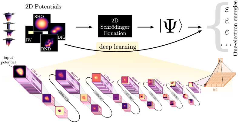
Figure 1: In this work, we use the machinery of deep learning to learn the mapping between potential and energy, bypassing the need to numerically solve the Schrödinger equation, and the need for computing wavefunctions. The architecture we used (shown here) consisted primarily of convolutional layers capable of extracting relevant features of the input potentials. Two fully-connected layers at the end serve as a decision layer, mapping the automatically extracted features to the desired output quantity. No manual feature-selection is necessary; this is a “featureless-learning” approach.

Such feature-based approaches are also being used in materials discovery Curtarolo et al. (2003); Hautier et al. (2010); Saad et al. (2012) to assist materials scientists in efficiently targeting their search at promising material candidates. Unsupervised learning techniques have been used to identify phases in many-body atomic configurations Wang (2016). In previous work, an artificial neural network was shown to interpolate the mapping of position to wavefunction for a specific electrostatic potential Monterola and Saloma (2003); Shirvany et al. (2008); Caetano et al. (2011), but the fit was not transferable, a limitation also present in other applications of artificial neural networks to partial differential equations van Milligen et al. (1995); Carleo and Troyer (2017). By transferable, we mean that a model trained on a particular form of partial differential equation will accurately and reliably predict results for examples of the same form (in our case, different confining potentials).

Machine learning can also be used to accelerate or bypass some of the heavy machinery of the ab initio method itself. In Snyder et al. (2012), the authors replaced the kinetic energy functional within density functional theory with a machine-learned one, and in Brockherde et al. (2016) and Yao and Parkhill (2016), the authors “learned” the mappings from potential to electron density, and charge density to kinetic energy, respectively.

Here, we use a fundamentally different approach inspired by the successful application of deep convolutional neural networks to problems in computer vision LeCun et al. (1998); Simard et al. (2003); Ciresan et al. (2011); Szegedy et al. (2015) and computational games Silver et al. (2016); Mnih et al. (2015). Rather than seeking an appropriate input representation to capture the relevant physical attributes of a system, we train a highly flexible model on an enormous collection of ground-truth examples. In doing so, the deep neural network learns both the features (in weight space) and the mapping required to produce the desired output. This approach does not depend on the appropriate selection of input representations and features; we provide the same data to both the deep neural network and the numerical method. As such, we call this “featureless learning”. Such an approach may offer a more scalable and parallizable approach to large-scale electronic structure problems than existing methods can offer.

In this Letter, we demonstrate the success of a featureless machine learning approach, a convolutional deep neural network, at learning the mapping between a confining electrostatic potential and quantities such as the ground state energy, kinetic energy, and first excited-state of a bound electron. The excellent performance of our model suggests deep learning as an important new direction for treating multi-electron systems in materials.

It is known that a sufficiently large artificial neural network can approximate any continuous mapping Funahashi (1989); Castro et al. (2000) but the cost of optimizing such a network can be prohibitive. Convolutional neural networks make computation feasible by exploiting the spatial structure of input data Alex et al. (2012), similar to how the neurons in the visual cortex function Hubel and Wiesel (1968). When multiple convolutional layers are included, the network is called a deep convolutional neural network, forming a hierarchy of feature detection Bengio (2009). This makes them particularly well suited to data rooted in physical origin Mehta and Schwab (2014); Lin et al. (2016), since many physical systems also display a structural hierarchy. Applications of such a network structure in the field of electronic structure, however, are few (although recent work focused on training against a geometric matrix representation looks particularly promising Schütt et al. (2017)).

II Methods

II.1 Training set: choice of potentials

Developing a deep learning model involves both the design of the network architecture and the acquisition of training data. The latter is the most important aspect of a machine learning model, as it defines the transferability of the resulting model. We investigated four classes of potentials: simple harmonic oscillators (SHO), “infinite” wells (IW, i.e. “particle in a box”), double-well inverted Gaussians (DIG), and random potentials (RND). Each potential can be thought of as a grayscale image: a grid of floating-point numbers.

II.2 Numerical solver

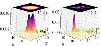
Figure 2: Wavefunctions (probability density) $|\psi_{0}|^{2}$ and the corresponding potentials $V(r)$ for two random potentials.

We implemented a standard finite-difference Frolkovič (1990) method to solve the eigenvalue problem

$$\hat{H}\psi\equiv(\hat{T}+\hat{V})\psi=\varepsilon\psi$$ (1)

for each potential $V$ we created. The potentials were generated with a dynamic range and length scale suitable to produce ground-state energies within a physically relevant range. With the random potentials, special care was taken to ensure that some training examples produced non-trivial wavefunctions (Fig. 2). Atomic units are used, such that $\hbar=m_{\mathrm{e}}=1$. The potentials are represented on a square domain from $-20$ to $20$ a.u., discretized on a $256\times 256$ grid. As the simple harmonic oscillator potentials have an analytic solution, we used this as reference with which to validate the accuracy of the solver. The median absolute error between the analytic and the calculated energies for all simple harmonic oscillator potentials was $0.12$ mHa. We discuss the generation of all potentials further in the Appendices.

The simple harmonic oscillator presents the simplest case for a convolutional neural network as there is an analytic solution dependent on two simple parameters ($k_{x}$ and $k_{y}$) which uniquely define the ground-state energy of a single electron ($\varepsilon_{0}=\frac{\hbar}{2}(\sqrt{k_{x}}+\sqrt{k_{y}})$). Furthermore, these parameters represent a very physical and visible quantity: the curvature of the potential in the two primary axes. Although these parameters are not provided to the neural network explicitly, the fact that a simple mapping exists means that the convolutional neural network need only learn it to accurately predict energies.

A similar situation exists for the infinite well. Like the simple harmonic oscillator, the ground state energy depends only on the width of the well in the two dimensions ($\varepsilon_{0}=\frac{1}{2}\pi^{2}\hbar^{2}(L_{x}^{-2}+L_{y}^{-2})$). It would be no surprise if even a modest network architecture is able to accurately “discover” this mapping. An untrained human, given a ruler, sufficient examples, and an abundance of time would likely succeed in determining this mapping.

The double-well inverted Gaussian dataset is more complex in two respects. First, the potential, generated by summing a pair of 2D-Gaussians, depends on significantly more parameters; the depth, width, and aspect ratio of each Gaussian, as well as the relative positions of the wells will impact the ground state energy. Furthermore, there is no known analytical solution for a single electron in a potential well of this nature. There is, however, still a concise function which describes the underlying potential, and while this is not directly accessible to the convolutional neural network, one must wonder if the existence of such simplifies the task of the convolutional neural network. Gaussian confining potentials appear in works relating to quantum dots Gharaati and Khordad (2010); Gomez and Romero (2008).

The random dataset presents the ultimate challenge. Each random potential is generated by a multi-step process with randomness introduced at numerous steps along the way. There is no closed-form equation to represent the potentials, and certainly not the eigenenergies. A convolutional neural network tasked with learning the solution to the Schrödinger equation through these examples would have to base its predictions on many individual features, truly “learning” the mapping of potential to energy. One might question our omission of the Coulomb potential as an additional canonical example. The singular nature of the Coulomb potential is difficult to represent within a finite dynamic range, and, more importantly, the electronic structure methods that we would ultimately seek to reproduce already have frameworks in place to deal with these singularities (e.g. pseudopotentials).

II.3 Deep neural network

Figure 3: The training loss curve for each model we trained. Since the training loss is based upon the training datasets, it does not necessarily indicate how well the model generalizes to new examples. The convergence seen here indicates that 1000 epochs is an adequate stopping point; further training would produce further reduction in loss, however 1000 epochs provides sufficient evidence that the method performs well on the most interesting (i.e. random) potentials. In the inset, we see that two non-reducing convolution layers is a consistent balance of training time and low error.

We chose to use a simple, yet deep neural network architecture (shown in Fig. 1) composed of a number of repeated units of convolutional layers, with sizes chosen for a balance of speed and accuracy (inset of Fig. 3).

We use two different types of convolutional layers, which we call “reducing” and “non-reducing”.

The 7 reducing layers operate with filter (kernel) sizes of $3\times 3$ pixels. Each reducing layer operates with 64 filters and a stride of $2\times 2$, effectively reducing the image resolution by a factor of two at each step. In between each pair of these reducing convolutional layers, we have inserted two convolutional layers (for a total of 12) which operate with $16$ filters of size $4\times 4$. These filters have unit stride, and therefore preserve the resolution of the image. The purpose of these layers is to add additional trainable parameters to the network. All convolutional layers have ReLU activation.

The final convolutional layer is fed into a fully-connected layer of width 1024, also with ReLU activation. This layer feeds into a final fully-connected layer with a single output. This output is the output value of the DNN. It is used to compute the mean-squared error between the true label and the predicted label, also known as the loss.

We used the AdaDelta Zeiler (2012) optimization scheme with a global learning rate of 0.001 to minimize this loss function (Fig. 3), monitoring its value as training proceeded. We found that after 1000 epochs (1000 times through all the training examples), the loss no longer decreased significantly.

We built a custom TensorFlow Abadi et al. (2016) implementation in order to make use of 4 graphical processing units (GPUs) in parallel. We placed a complete copy of the neural network on each of the 4 GPUs, so that each can compute a forward and back-propagation iteration on one full batch of images. Thus our effective batch size was 1000 images per iteration (250 per GPU). After each iteration, the GPUs share their independently computed gradients with the optimizer and the optimizer moves the parameters in the direction that minimizes the loss function. Unless otherwise specified, all training datasets consisted of 200,000 training examples and training was run for 1000 epochs. All reported errors are based on evaluating the trained model on validation datasets consisting of 50,000 potentials not accessible to the network during the training process.

III Results

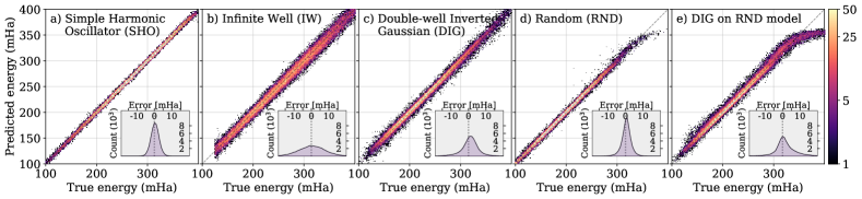
Figure 4: Histograms of the true vs. predicted energies for each example in the test set indicate the performance of the various models. The insets show the distribution of error away from the diagonal line representing perfect predictions. A $1\ \text{mHa}^{2}$ square bin is used for the main histograms, and a 1 mHa bin size for the inset histogram. During training, the neural network was not exposed to the examples on which theses plots are based. The higher error at high energies in (d) is due to fewer training examples being present the dataset at these energies. The histogram shown in (d) is for the further-trained model, described in the text.

Fig. 4(a-d) displays the results for the simple harmonic oscillator, infinite well, double-well inverted Gaussian, and random potentials. The simple harmonic oscillator, being one of the simplest potentials, performed extremely well. The trained model was able to predict the ground state energies with a median absolute error (MAE) of 1.51 mHa.

The infinite well potentials performed moderately well with a MAE of 5.04 mHa. This is notably poorer than the simple harmonic oscillator potentials, despite their similarity in being analytically dependent upon two simple parameters. This is likely due to the sharp discontinuity associated with the infinite well potentials, combined with the sparsity of information present in the binary-valued potentials.

The model trained on the double-well inverted Gaussian potentials performed moderately well with a MAE of 2.70 mHa and the random potentials performed quite well with a MAE of 2.13 mHa. We noticed, however, that the loss was not completely converged at 1000 epochs, so we provided an additional 200,000 training examples to the network and allowed it to train for an additional 1000 epochs. With this added training, the the model performed exceptionally well, with a MAE of 1.49 mHa, below the threshold of chemical accuracy (1 kcal/mol, 1.6 mHa). In Fig. 4(d), it is evident that the model performs more poorly at high energies, a result of the relative absence of high-energy training examples in the dataset. Given the great diversity in this latter set of potentials, it is impressive that the convolutional neural network was able to learn how to predict the energy with such a high degree of accuracy.

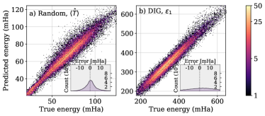
Figure 5: Histograms of the true vs. predicted energies for the model trained on the (a) kinetic energy, and (b) excited-state energy of the double-well inverted Gaussian.

Now that we have a trained model that performs well on the random test set, we investigated its transferability to another class of potentials. The model trained on the random dataset is able to predict the ground-state energy of the double-well inverted Gaussian potentials with a MAE of 2.94 mHa. We can see in Fig. 5(c) that the model fails at high energies, an expected result given that the model was not exposed to many examples in this energy regime during training on the overall lower-energy random dataset. This moderately good performance is not entirely surprising; the production of the random potentials includes an element of Gaussian blurring, so the neural network would have been exposed to features similar to what it would see in the double-well inverted Gaussian dataset. However, this moderate performance is testament to the transferability of convolutional neural network models. Furthermore, we trained a model on an equal mixture of all four classes of potentials. It performs moderately with a MAE of 5.90 mHa. This error could be reduced through further tuning of the network architecture allowing it to better capture the higher variation in the dataset.

The total energy is just one of the many quantities associated with these one-electron systems. To demonstrate the applicability of deep neural network to other quantities, we trained a model on the first excited-state energy $\varepsilon_{1}$ of the double-well inverted Gaussian potentials. The model achieved a MAE of 10.93 mHa. We now have two models capable of predicting the ground-state, and first excited-state energies separately, demonstrating that a neural network can learn quantities other than the ground-state energy.

The ground-state and first excited-state are both eigenvalues of the Hamiltonian. Therefore, we investigated the training of a model on the expectation value of the kinetic energy, $\langle\hat{T}\rangle=\langle\psi_{0}|\hat{T}|\psi_{0}\rangle$, under the ground state wavefunction $\psi_{0}$ that we computed numerically for the random potentials. Since $\hat{H}$ and $\hat{T}$ do not commute, the prediction of $\langle\hat{T}\rangle$ can no longer be summarized as an eigenvalue problem. The trained model predicts the kinetic energy value with a MAE of 2.98 mHa. While the spread of testing examples in Fig. 5(a) suggests the model performs more poorly, the absolute error is still small.

IV Conclusions

We note that many other machine learning algorithms exist and have traditionally seen great success, such as kernel ridge regression Brockherde et al. (2016); Arsenault et al. (2014); Li et al. (2016); Suzuki et al. (2017); Faber et al. (2017); Lopez-Bezanilla and von Lilienfeld (2014) and random forests Faber et al. (2017); Ward et al. (2015). Like these algorithms, convolutional deep neural networks have the ability to “learn” relevant features and form a non-linear input-to-output mapping without prior formulation of an input representation Kearnes et al. (2016); Schütt et al. (2017). In our tests, these methods perform more poorly and scale such that a large number of training examples is infeasible. We have included a comparison of these alternative machine learning methods in the Appendices, justifying our decision of using a deep convolutional neural network. One notable limitation of our approach is that the efficient training and evaluation of the deep neural network requires uniformity in the input size. Future work will focus on an approach that would allow transferability to variable input sizes.

Additionally, an electrostatic potential defined on a finite grid can be rotated in integer multiples of $90\mathrm{°}$, without a change to the electrostatic energies. Convolutional deep neural networks do not natively capture such rotational invariance. Clearly, this is a problem in any application of deep neural networks (e.g. image classification, etc.), and various techniques are used to compensate for the desired invariance. The common approach is to train the network on an augmented dataset consisting both of the original training set and rotated copies of the training data Dieleman et al. (2015). In this way, the network learns a rotationally invariant set of features.

In demonstration of this technique, we tuned our model trained on the random potentials by training it further on an augmented dataset of rotated random potentials. We then tested our model on the original testing dataset, as well as a rotated copy of the test set. The median absolute error in both cases was less than 1.6 mHa. The median absolute difference in predicted energy between the rotated and unaltered test sets was however larger, at 1.7 mHa. This approach to training the deep neural network is not absolutely rotationally invariant, however the numerical error experienced due to a rotation was on the same order as the error of the method itself. Recent proposals to modify the network architecture itself to make it rotationally invariant are promising, as the additional training cost incurred with using an augmented dataset could be avoided Worrall et al. (2016); Dieleman et al. (2016).

In summary, convolutional deep neural networks are promising candidates for application to electronic structure calculations as they are designed for data which has a spatial encoding of information. As the number of electrons in a system increases, the computational complexity grows polynomially. Accurate electronic structure methods (e.g. coupled cluster) exhibit a scaling with respect to the number of particles of $N^{7}$ and even the popular Kohn-Sham formalism of density functional theory scales as $N^{3}$ Kohn (1995); Kucharski and Bartlett (1992). The evaluation of a convolutional neural network exhibits no such scaling, and while the training process for more complicated systems would be more expensive, this is a one-time cost.

In this work, we have taken a simple problem (one electron in a confining potential), and demonstrated that a convolutional neural network can automatically extract features and learn the mapping between $V(r)$ and the ground-state energy $\varepsilon_{0}$ as well as the kinetic energy $\langle\hat{T}\rangle$, and first excited-state energy $\varepsilon_{1}$. Although our focus here has been on a particular type of problem, namely an electron in a confining 2D well, the concepts here are directly applicable to many problems in physics and engineering. Ultimately, we have demonstrated the ability of a deep neural network to learn, through example alone, how to rapidly approximate the solution to a set of partial differential equations. A generalizable, transferable deep learning approach to solving partial differential equations would impact all fields of theoretical physics and mathematics.

V Acknowledgements

The authors would like to acknowledge fruitful discussions with P. Bunker, P. Darancet, D. Klug, and D. Prendergast. K.M. and I.T. acknowledge funding from NSERC and SOSCIP. Compute resources were provided by SOSCIP, Compute Canada, NRC, and an NVIDIA Faculty Hardware Grant.

Appendix A Appendices

A.1 Appendix A: Comparison of machine learning methods

One might question the use of a convolutional deep neural network over other more traditional machine learning approaches. After all, kernel ridge regression, random forests, and artificial neural networks have proven to be quite useful (see main work for references to appropriate work). Here we compare the use of our convolutional deep neural network approach to kernel ridge regression and random forests, the latter two implemented through Scikit-learn Pedregosa et al. (2012).

A.1.1 Kernel ridge regression

We trained a kernel ridge regression model on a training set of simple harmonic oscillator images, recording the walltime (real-world time) taken to train the model. Then we evaluated the trained model on a test set (the same test set was used throughout). We recorded both the evaluation walltime and the median absolute error (MAE) observed from the trained model. We then trained our deep neural network on the same training dataset, allowing it the same training walltime as the KRR model. We then evaluated the deep neural network on the same testing set of data, again recording the MAE and the evaluation walltime. This process was repeated for various training set sizes, and on training data from both the simple harmonic oscillator (SHO) and random (RND) datasets. The results are presented in Fig. 6 and Fig. 7.

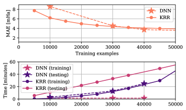
Figure 6: Kernel ridge regression on simple harmonic oscillator potentials. When few training examples are provided, kernel ridge regression performs better, however with a larger number of training examples, both methods perform comparably, with DNN slightly better. The training time for kernel ridge regression scales quadratically. The evaluation time for a fixed number of testing examples scales linearly with respect to the number of training examples in the case of kernel ridge regression. In the case of the deep neural network, the training set size does not affect the testing set evaluation.

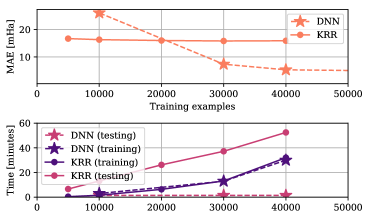
Figure 7: Kernel ridge regression on random potentials. When few training examples are present, kernel ridge regression performs better (at constant training time). This is likely due to the fact that the DNN is only given 10 seconds to run. At larger training set sizes, the deep neural network performs much better; kernel ridge regression barely improves as training set size increases, however training walltime increases dramatically.

A.1.2 Random forests

We carried out an identical process, training a random forests regressor. The results are presented in Fig. 8 and Fig. 9.

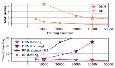
Figure 8: Random forests and simple harmonic oscillator. Random forests performs better than deep neural networks for all training set sizes on the relatively trivial simple harmonic oscillator dataset. Random forests takes a very long time to train. Note that the training times plotted above have been scaled by a factor of 0.1 for plotting, and thus the true times are ten times greater than shown.

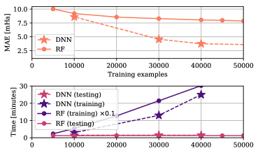
Figure 9: Random forests on random potentials. On the more complicated random potentials, random forests performs significantly worse than the deep neural network. This combined with the extremely high training time suggests the deep neural network is much better equipped to handle these more varied potentials.

A.1.3 Discussion

While the timing comparison is not quantitatively fair (the random forests algorithm is not parallelized and uses only one CPU core. The kernel ridge regression algorithm is parallelized and ran across all available cores, and the deep neural network is highly parallelized via GPU optimization, and runs across thousands of cores), this investigation gives useful insight into the time-to-solution advantages of deep neural networks. The error rates, however are quantitatively comparable, as the KRR and RF algorithms were permitted to run until convergence. The DNN was able to perform better in most cases given the same amount of walltime.

We see that for all but the simplest cases, our deep neural network is vastly superior to both kernel ridge regression and random forests. For very simple potentials, it is understandable that the machinery of the deep neural network was unnecessary, and that the traditional methods perform well. For more complicated potentials with more variation in the input data, the deep neural network was able to provide significantly better accuracy in the same amount of time.

A.2 Appendix B: Dataset generation

The potentials are defined on a grid from $x,y=-20$ to $20$ a.u. on a $256\times 256$ grid.

A.2.1 Simple Harmonic Oscillator

The simple harmonic oscillator (SHO) potentials are generated with with the scalar function

$$V(x,y)=\frac{1}{2}\left(k_{x}(x-c_{x})^{2}+k_{y}(y-c_{y})^{2}\right)$$ (2)

where $k_{x},k_{y},c_{x}$, and $c_{y}$ are randomly generated according to Table 1. The potentials are truncated at 20.0 Ha, (i.e. if $V>20$, $V=20$).

Table 1:

Parameter		Lower bound	Upper bound
$k_{x}$	spring constant	0.0	0.16
$k_{y}$	spring constant	0.0	0.16
$c_{x}$	center position	-8.0	8.0
$c_{y}$	center position	-8.0	8.0

A.2.2 Infinite Well

The infinite well (IW) potentials are generated with the scalar function

$$V(x,y)=\begin{cases}0&\frac{1}{2}\left(2c_{x}-L_{x}\right)<x\leq\frac{1}{2}\left(2c_{x}+L_{x}\right)\ \text{and}\\ &\frac{1}{2}\left(2c_{y}-L_{y}\right)<y\leq\frac{1}{2}\left(2c_{y}+L_{y}\right)\\ 20&\text{otherwise}\\ \end{cases}$$ (3)

where 20.0 is used as “numerical infinity”, an appropriate choice given the scale of energies used. Because of the nature of the IW energy, randomly generating $L_{x}$ and $L_{y}$ independently leads to a distribution of eneries highly biased toward low energy values (it is more likely to randomly produce a large well than a small). Since we want a distribution that is as even as possible over the range of energies, we need to take a slightly different approach. We randomly generate the energy $E$ uniformly on the interval 0 to 0.4 Ha. We then generate $L_{x}$ randomly on the interval 4.0 to 15.0, defining the width of the well. We then solve for the value of $L_{y}$ that will produce an energy of $E$, given $L_{x}$, e.g.

$$L_{y}=1/\sqrt{\frac{2E}{\pi^{2}}-\frac{1}{L_{x}^{2}}}$$ (4)

Not all combinations of $L_{x}$ and $E$ lead to valid solutions for $L_{y}$, so we keep trying until one does. We then swap the values of $L_{x}$ and $L_{y}$ with a 50% probability to prevent one dimension of the well always being larger. This process leads to a relatively even distribution of energies.

A.2.3 Double-well inverted Gaussians

The double-well inverted Gaussian (DIG) potentials are generated with the scalar function

$$V(x,y)=-A_{1}\exp\left[-\left(\frac{x-c_{x_{1}}}{k_{x_{1}}}\right)^{2}-\left(\frac{y-c_{y_{1}}}{k_{y_{1}}}\right)^{2}\right]\\ -A_{2}\exp\left[-\left(\frac{x-c_{x_{2}}}{k_{x_{2}}}\right)^{2}-\left(\frac{y-c_{y_{2}}}{k_{y_{2}}}\right)^{2}\right]$$ (5)

where the parameters are randomly sampled from a uniform distribution within the ranges given in Table 2. These ranges were determined through trial and error to achieve energies in the range of 0 to 400 mHa.

Table 2:

Parameter		Lower bound	Upper bound
$A_{1}$	well 1 depth	2.0	4.0
$A_{2}$	well 2 depth	2.0	4.0
$c_{x_{1}}$	well 1 center, $x$	-8.0	8.0
$c_{y_{1}}$	well 1 center, $y$	-8.0	8.0
$c_{x_{2}}$	well 2 center, $x$	-8.0	8.0
$c_{y_{2}}$	well 2 center, $y$	-8.0	8.0
$k_{x_{1}}$	well 1 width	1.6	8.0
$k_{y_{1}}$	well 1 length	1.6	8.0
$k_{x_{2}}$	well 2 width	1.6	8.0
$k_{y_{2}}$	well 2 length	1.6	8.0

A.2.4 Random potentials

The random potentials are generated through a lengthy process motivated by three requirements: the potentials must (a) be random (i.e. extremely improbable that two identical potentials ever be generated), (b) be smooth, and (c) go to a maximum of 20.0 at the boundary.

First, we generate a $16\times 16$ binary grid of 1s and 0s, and upscale it to $256\times 256$. We then generate a second $16\times 16$ binary grid and and upscale it to $128\times 128$. We center the smaller grid within the larger grid and then subtract them element-wise. We then apply a Gaussian blur with standard deviation $\sigma_{1}$, to the resulting image, where $\sigma_{1}$ is generated uniformly within the range given in Table 3. The potential is now random, and smooth, but does not achieve a maximum at the boundary.

To achieve this, we generate a mask that smoothly goes to zero at the boundary, and 1 in the interior. We wish the mask to be random, e.g. a randomly generated ‘blob’. To generate the blob, we generate $k^{2}$ random coordinate pairs on a $200\times 200$ grid, where $k$ is an integer between 2 and 7, inclusive. We then throw away all points that lie inside the covex hull of these points, and smoothly interpolate the remaining points with cubic splines. We then form a binary mask by filling the inside of this closed blob with 1s, and the outside with 0s. Resizing the blob to a resolution of $R\times R$, and applying a Gaussian blur with standard deviation $\sigma_{2}$, we arrive at the final mask. Here $R$ and $\sigma_{2}$ are generated uniformly within the ranges given in Table 3.

Element-wise multiplication of the mask with the random-blurred image gives a random potential that approaches zero at the boundary. We randomize the “sharpness” of the potential by then exponentiating by either $d=0.1,0.5,1.0,\text{or}2.0$, chosen at random with equal probabilities (i.e. $V:=V^{d}$). We then subtract the result from its maximum to invert the well.

This process, while lengthy, produces very random potentials, of which no two are alike. The energy range of 0 to 400 mHa is appropriate for producing wavefunctions that span a moderate portion of the domain, as seen in Fig. 10. Examples of all classes of potentials can be seen in Fig. 11.

Table 3:

Parameter		Lower bound	Upper bound
$\sigma_{1}$	std. dev. blur 1	6	10
$k$	blob points	2	7
$R$	blob size	80	180
$\sigma_{2}$	std. dev. blur 2	10	16

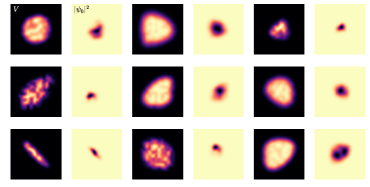
Figure 10: Some example random potentials $V$ and the norm of their associated ground-state wavefunctions, $|\psi_{0}|^{2}$.

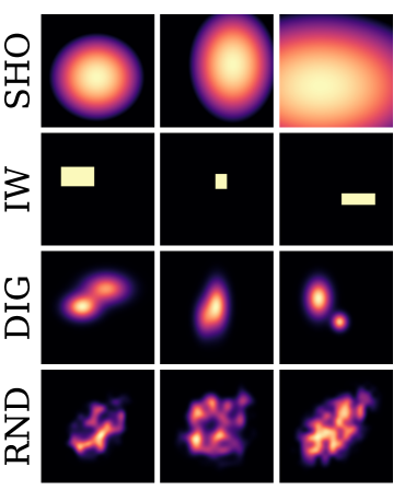
Figure 11: Examples of the four classes of potentials

References

- Dirac (1929) P. A. M. Dirac, Royal Society 123, 714 (1929).
- Cherukara et al. (2016) M. J. Cherukara, B. Narayanan, A. Kinaci, K. Sasikumar, S. K. Gray, M. K. Chan, and S. K. R. S. Sankaranarayanan, The Journal of Physical Chemistry Letters 7, 3752 (2016).
- Riera et al. (2016) M. Riera, A. W. Götz, and F. Paesani, Physical Chemistry Chemical Physics 18, 30334 (2016).
- Jaramillo-Botero et al. (2014) A. Jaramillo-Botero, S. Naserifar, and W. A. Goddard, Journal of Chemical Theory and Computation 10, 1426 (2014).
- Van Beest et al. (1990) B. W. H. Van Beest, G. J. Kramer, and R. A. Van Santen, Physical Review Letters 64, 1955 (1990).
- Ponder and Case (2003) J. W. Ponder and D. A. Case, Advances in Protein Chemistry 66, 27 (2003).
- Hornak et al. (2006) V. Hornak, R. Abel, A. Okur, B. Strockbine, A. Roitberg, and C. Simmerling, Proteins: Structure, Function, and Bioinformatics 65, 712 (2006), arXiv:0605018 [q-bio] .
- Cole et al. (2007) D. J. Cole, M. C. Payne, G. Csányi, S. Mark Spearing, and L. Colombi Ciacchi, The Journal of Chemical Physics 127, 204704 (2007), arXiv:0807.3215 .
- van der Waals (1873) van der Waals, De continuiteit van den gasen Vloeistoftoestand, Ph.D. thesis (1873).
- Li et al. (2013) H. Z. Li, L. Li, Z. Y. Zhong, Y. Han, L. Hu, and Y. H. Lu, Mathematical Problems in Engineering 2013, 1 (2013).
- Behler and Parrinello (2007) J. Behler and M. Parrinello, Physical Review Letters 98, 1 (2007).
- Morawietz and Behler (2013) T. Morawietz and J. Behler, Journal of Physical Chemistry A 117, 7356 (2013).
- Behler et al. (2008) J. Behler, R. Martoňák, D. Donadio, and M. Parrinello, physica status solidi (b) 245, 2618 (2008).
- Dolgirev et al. (2016) P. E. Dolgirev, I. A. Kruglov, and A. R. Oganov, AIP Advances 6, 085318 (2016).
- Artrith and Urban (2016) N. Artrith and A. Urban, Computational Materials Science 114, 135 (2016).
- Tian et al. (2017) W. Tian, F. Meng, L. Liu, Y. Li, and F. Wang, Scientific Reports 7, 40827 (2017).
- Rupp et al. (2012) M. Rupp, A. Tkatchenko, K. R. Müller, and O. A. von Lilienfeld, Physical Review Letters 108, 058301 (2012).
- Faber et al. (2017) F. A. Faber, L. Hutchison, B. Huang, J. Gilmer, S. S. Schoenholz, G. E. Dahl, O. Vinyals, S. Kearnes, P. F. Riley, and O. A. von Lilienfeld, arXiv , 1 (2017), arXiv:1702.05532 .
- Montavon et al. (2013) G. Montavon, M. Rupp, V. Gobre, A. Vazquez-Mayagoitia, K. Hansen, A. Tkatchenko, K. R. Müller, and O. Anatole von Lilienfeld, New Journal of Physics 15, 095003 (2013), arXiv:1305.7074 .
- Lopez-Bezanilla and von Lilienfeld (2014) A. Lopez-Bezanilla and O. A. von Lilienfeld, Physical Review B 89, 235411 (2014), arXiv:1401.8277 .
- Jia et al. (2014) Y. Jia, E. Shelhamer, J. Donahue, S. Karayev, J. Long, R. Girshick, S. Guadarrama, and T. Darrell, arXiv , 675 (2014), arXiv:1408.5093 .
- Curtarolo et al. (2003) S. Curtarolo, D. Morgan, K. Persson, J. Rodgers, and G. Ceder, Physical Review Letters 91, 135503 (2003), arXiv:0307262 [cond-mat] .
- Hautier et al. (2010) G. Hautier, C. C. Fischer, A. Jain, T. Mueller, and G. Ceder, Chemistry of Materials 22, 3762 (2010).
- Saad et al. (2012) Y. Saad, D. Gao, T. Ngo, S. Bobbitt, J. R. Chelikowsky, and W. Andreoni, Physical Review B 85, 104104 (2012).
- Wang (2016) L. Wang, Physical Review B 94, 195105 (2016), arXiv:1606.00318 .
- Monterola and Saloma (2003) C. Monterola and C. Saloma, Optics Communications 222, 331 (2003).
- Shirvany et al. (2008) Y. Shirvany, M. Hayati, and R. Moradian, Communications in Nonlinear Science and Numerical Simulation 13, 2132 (2008).
- Caetano et al. (2011) C. Caetano, J. L. Reis, J. Amorim, M. R. Lemes, and A. D. Pino, International Journal of Quantum Chemistry 111, 2732 (2011).
- van Milligen et al. (1995) B. P. van Milligen, V. Tribaldos, and J. A. Jiménez, Physical Review Letters 75, 3594 (1995).
- Carleo and Troyer (2017) G. Carleo and M. Troyer, Science 355, 602 (2017).
- Snyder et al. (2012) J. C. Snyder, M. Rupp, K. Hansen, K.-R. Müller, and K. Burke, Physical Review Letters 108, 253002 (2012).
- Brockherde et al. (2016) F. Brockherde, L. Vogt, L. Li, M. E. Tuckerman, K. Burke, and K.-R. Müller, arXiv , 1 (2016), arXiv:1609.02815 .
- Yao and Parkhill (2016) K. Yao and J. Parkhill, Journal of Chemical Theory and Computation 12, 1139 (2016), arXiv:1509.00062 .
- LeCun et al. (1998) Y. LeCun, L. Bottou, Y. Bengio, and P. Haffner, Proceedings of the IEEE 86, 2278 (1998), arXiv:1102.0183 .
- Simard et al. (2003) P. Simard, D. Steinkraus, and J. Platt, in Seventh International Conference on Document Analysis and Recognition, 2003. Proceedings., Vol. 1 (IEEE Comput. Soc, 2003) pp. 958–963.
- Ciresan et al. (2011) D. C. Ciresan, U. Meier, J. Masci, L. M. Gambardella, J. Schmidhuber, D. C. Cireşan, U. Meier, J. Masci, L. M. Gambardella, and J. Schmidhuber, in Proceedings of the 22nd International Joint Conference on Artificial Intelligence, Vol. 22 (2011) pp. 1237–1242.
- Szegedy et al. (2015) C. Szegedy, W. Liu, Y. Jia, P. Sermanet, S. Reed, D. Anguelov, D. Erhan, V. Vanhoucke, and A. Rabinovich, in Proceedings of the IEEE Computer Society Conference on Computer Vision and Pattern Recognition, Vol. 07-12-June (IEEE, 2015) pp. 1–9, arXiv:1409.4842 .
- Silver et al. (2016) D. Silver, A. Huang, C. J. Maddison, A. Guez, L. Sifre, G. van den Driessche, J. Schrittwieser, I. Antonoglou, V. Panneershelvam, M. Lanctot, S. Dieleman, D. Grewe, J. Nham, N. Kalchbrenner, I. Sutskever, T. Lillicrap, M. Leach, K. Kavukcuoglu, T. Graepel, and D. Hassabis, Nature 529, 484 (2016).
- Mnih et al. (2015) V. Mnih, K. Kavukcuoglu, D. Silver, A. a. Rusu, J. Veness, M. G. Bellemare, A. Graves, M. Riedmiller, A. K. Fidjeland, G. Ostrovski, S. Petersen, C. Beattie, A. Sadik, I. Antonoglou, H. King, D. Kumaran, D. Wierstra, S. Legg, and D. Hassabis, Nature 518, 529 (2015).
- Funahashi (1989) K. I. Funahashi, Neural Networks 2, 183 (1989).
- Castro et al. (2000) J. L. Castro, C. J. Mantas, and J. M. Benítez, Neural Networks 13, 561 (2000).
- Alex et al. (2012) K. Alex, I. Sutskever, and G. E. Hinton, in Neural Information Processing Systems (NIPS) (2012) pp. 1097–1105.
- Hubel and Wiesel (1968) D. H. Hubel and T. N. Wiesel, The Journal of Physiology 195, 215 (1968).
- Bengio (2009) Y. Bengio, Foundations and Trends in Machine Learning 2, 1 (2009).
- Mehta and Schwab (2014) P. Mehta and D. J. Schwab, arXiv , 1 (2014), arXiv:1410.3831 .
- Lin et al. (2016) H. W. Lin, M. Tegmark, and D. Rolnick, arXiv 86, 2278 (2016), arXiv:1608.08225 .
- Schütt et al. (2017) K. T. Schütt, F. Arbabzadah, S. Chmiela, K. R. Müller, and A. Tkatchenko, Nature Communications 8, 13890 (2017).
- Frolkovič (1990) P. Frolkovič, Acta Applicandae Mathematicae, 3rd ed., Vol. 19 (Cambridge University Press, New York, NY, USA, 1990) pp. 297–299.
- Gharaati and Khordad (2010) A. Gharaati and R. Khordad, Superlattices and Microstructures 48, 276 (2010).
- Gomez and Romero (2008) S. S. Gomez and R. H. Romero, 5500, 14 (2008), arXiv:0804.1961 .
- Zeiler (2012) M. D. Zeiler, arXiv , 6 (2012), arXiv:1212.5701 .
- Abadi et al. (2016) M. Abadi, A. Agarwal, P. Barham, E. Brevdo, Z. Chen, C. Citro, G. S. Corrado, A. Davis, J. Dean, M. Devin, S. Ghemawat, I. Goodfellow, A. Harp, G. Irving, M. Isard, Y. Jia, R. Jozefowicz, L. Kaiser, M. Kudlur, J. Levenberg, D. Mane, R. Monga, S. Moore, D. Murray, C. Olah, M. Schuster, J. Shlens, B. Steiner, I. Sutskever, K. Talwar, P. Tucker, V. Vanhoucke, V. Vasudevan, F. Viegas, O. Vinyals, P. Warden, M. Wattenberg, M. Wicke, Y. Yu, and X. Zheng, None 1, 19 (2016), arXiv:1603.04467 .
- Arsenault et al. (2014) L. F. Arsenault, A. Lopez-Bezanilla, O. A. von Lilienfeld, and A. J. Millis, Physical Review B 90, 155136 (2014), arXiv:1408.1143 .
- Li et al. (2016) L. Li, J. C. Snyder, I. M. Pelaschier, J. Huang, U.-N. Niranjan, P. Duncan, M. Rupp, K.-R. Müller, and K. Burke, International Journal of Quantum Chemistry 116, 819 (2016), arXiv:1404.1333v2 .
- Suzuki et al. (2017) T. Suzuki, R. Tamura, and T. Miyazaki, International Journal of Quantum Chemistry 117, 33 (2017), arXiv:1608.07374 .
- Ward et al. (2015) L. Ward, A. Agrawal, A. Choudhary, and C. Wolverton, Nature Communications 2, 1 (2015), arXiv:1606.09551 .
- Kearnes et al. (2016) S. Kearnes, K. McCloskey, M. Berndl, V. Pande, and P. Riley, Journal of Computer-Aided Molecular Design 30, 595 (2016), arXiv:1603.00856 .
- Dieleman et al. (2015) S. Dieleman, K. W. Willett, and J. Dambre, Monthly Notices of the Royal Astronomical Society 450, 1441 (2015), arXiv:1503.07077 .
- Worrall et al. (2016) D. E. Worrall, S. J. Garbin, D. Turmukhambetov, and G. J. Brostow, (2016), arXiv:1612.04642 .
- Dieleman et al. (2016) S. Dieleman, J. De Fauw, and K. Kavukcuoglu, (2016), arXiv:1602.02660 .
- Kohn (1995) W. Kohn, International Journal of Quantum Chemistry 56, 229 (1995).
- Kucharski and Bartlett (1992) S. A. Kucharski and R. J. Bartlett, The Journal of Chemical Physics 97, 4282 (1992).
- Pedregosa et al. (2012) F. Pedregosa, G. Varoquaux, A. Gramfort, V. Michel, B. Thirion, O. Grisel, M. Blondel, G. Louppe, P. Prettenhofer, R. Weiss, V. Dubourg, J. Vanderplas, A. Passos, D. Cournapeau, M. Brucher, M. Perrot, and É. Duchesnay, Journal of Machine Learning Research 12, 2825 (2012), arXiv:1201.0490 .