Inhomogeneous chiral condensate in the quark-meson model

Abstract

The two-flavor quark-meson model is used as a low-energy effective model for QCD to study inhomogeneous chiral condensates at finite baryon chemical potential $\mu_{B}$. The parameters of the model are determined by matching the meson and quark masses, and the pion decay constant to their physical values using the on-shell and modified minimal subtraction schemes. Using a chiral-density wave ansatz for the inhomogeneity, we calculate the effective potential in the mean-field approximation and the result is completely analytic. The size of the inhomogeneous phase depends sensitively on the pion mass and whether one includes the vacuum fluctuations or not. Finally, we briefly discuss the mean-field phase diagram.

I Introduction

The phase structure of QCD has been subject of interest since its phase diagram was first conjectured in the 1970s. Today, we have a relatively good understanding of the phase transition at zero baryon chemical potential $\mu_{B}$. At $\mu_{B}=0$ there is no sign problem and one can use lattice simulations. For 2+1 flavors and physical quark masses, the transition is a crossover at a temperature of around 155 MeV aoki1 ; aoki2 ; borsa ; baza . Above the transition temperature QCD is in the quark-gluon plasma phase. At temperatures up to a few times the transition temperature, this is a strongly interacting liquid kris . For higher temperatures, resummed perturbation theory yields results for the thermodynamic functions that are in good agreement with lattice data hon1 ; hon2 .

The situation is less clear at finite density and low temperature. Due to the sign problem, this part of the phase diagram is not accessible to standard Monte Carlo techniques based on importance sampling. Only at asymptotically high densities are we confident about the phase and the properties of QCD. In this limit, the ground state of QCD is the color-flavor locked phase which is a color-superconducting phase rev1 . The color symmetry is completely broken and all the gluons are screened. The low-energy excitations of this phase are Goldstone modes which can be described by a chiral effective Lagrangian. At medium densities, information about the phase diagram has been obtained mainly by using low-energy effective models that share some features with QCD such as chiral symmetry breaking in the vacuum. Examples of low-energy models are the Nambu-Jona-Lasinio (NJL) model and the quark-meson (QM) model as well as their Polyakov-loop extended versions PNJL and PQM models.

Details and further motivation of the QM model can be found in zuber and GellMann , although historically the fermionic degrees of freedom were nucleons instead of quarks. One may object to having both quark and mesonic degrees of freedom present at the same time in the QM model, since quarks are confined at low temperatures. The Polyakov loop is introduced in order to mimic confinement in QCD in a statistical sense by coupling the chiral models to a constant $SU(N_{c})$ background gauge field $A_{\mu}^{a}$ fukushima , which is expressed in terms of the complex-valued Polyakov loop variable $\Phi$. Consequently the effective potential becomes a function of the expectation value of the chiral condensate and the expectation value of the Polykov loop, where the latter then serves as an approximate order parameter for confinement. Finally, one adds the contribution to the free energy density from the gluons via a phenomenological Polyakov loop potential fukushima .

At these lower densities, QCD is still in a color-superconducting phase, but the symmetry-breaking pattern is different rev1 ; rev2 . The ground state for a given value of the baryon chemical potential is very sensitive to the values of the parameters of the effective models. It turns out that some of the color-superconducting phases are inhomogeneous rev1 ; rev2 ; suprev . Inhomogeneous phases do not exist only in dense QCD, but also for example in ordinary superconductors and in imbalanced Fermi gases. In the present paper, we reconsider the problem of inhomogeneous chiral-symmetry breaking phases in dense QCD buballarev ; robd within the QM model. To be specific, we focus on a chiral-density wave (CDW). The problem of inhomogeneous phases has been addressed before in the context of the Ginzburg-Landau approach nick2 ; abuki ; friman ; japs , the NJL nakano ; mada ; nickel ; vari ; dirk ; lee2 and PNJL models nickel2 ; brun , the QM model nickel ; bubsc ; fix1 , and the nonlocal chiral quark model scoc . Numerical methods for the calculation of the phase diagram for a general inhomogeneous condensate are available forcrand ; wagner , but we resort to a chiral-density wave ansatz in order to present analytical results.

Most of the work has been done in the mean-field approximation; however, the properties of the Goldstone modes that are associated with the spontaneous symmetry breaking of space-time symmetries are important as they may destabilize the inhomogeneous phase friman ; japs . The destabilization is caused by long-wavelength fluctuations at finite temperature, where long-range order is replaced by algebraic decay of the order parameter. This does not apply at $T=0$ since the long-wavelength fluctuations are suppressed in this case.

In the next section, we briefly discuss the QM model and explain how we calculate the one-loop effective potential in the large-$N_{c}$ limit using the on-shell (OS) and modified minimal subtraction ($\overline{\rm MS}$) schemes together with dimensional regularization. We also calculate analytically the medium-dependent part of the effective potential and the quark density at zero temperature. In Sec. III, we present and discuss our results for the different phases. We also discuss the mean-field phase diagram as a function of $T$ and $\mu$. In Appendix A we calculate some integrals and sum-integrals that we need, and in Appendix B, we calculate the parameters of the Lagrangian as functions of physical observables to leading order in the large-$N_{c}$ expansion. Finally, in Appendix C, we calculate the effective potential to the same order.

II Quark-meson model and effective potential

The Euclidean Lagrangian of the two-flavor quark-meson model is

$${\cal L} = {1\over 2}\left[(\partial_{\mu}\sigma)^{2}+(\partial_{\mu}{\bm{\pi}})^{2}\right]+{1\over 2}m^{2}(\sigma^{2}+{\bm{\pi}}^{2})$$ (1)

$$+{\lambda\over 24}(\sigma^{2}+{\bm{\pi}}^{2})^{2}-h\sigma$$

$$+\bar{\psi}_{f}\left[/\!\!\!\partial-\gamma^{0}\mu_{f}+g(\sigma+i\gamma^{5}{\bm{\tau}}\cdot{\bm{\pi}})\right]\psi_{f}\;,$$

where $f=u,d$ is the flavor index and $\mu_{f}$ is the corresponding chemical potential. For $\mu_{u}=\mu_{d}$, in addition to a global $SU(N_{c})$ symmetry, the Lagrangian has a $U(1)_{B}\times SU(2)_{L}\times SU(2)_{R}$ symmetry in the chiral limit, while away from it, the symmetry is reduced to $U(1)_{B}\times SU(2)_{V}$. For $\mu_{u}\neq\mu_{d}$, the symmetry is reduced to $U(1)_{B}\times U(1)_{I_{3}L}\times U(1)_{I_{3}R}$ for $h=0$ and $U(1)_{B}\times U(1)_{I_{3}}$ for $h\neq 0$. In the remainder of this paper we choose $\mu_{u}=\mu_{d}=\mu={1\over 3}\mu_{B}$, where $\mu$ is the quark chemical potential and $\mu_{B}$ is the baryon chemical potential.

In the vacuum, the $\sigma$ field acquires a nonzero vacuum expectation value, which we denote by $\phi_{0}$. We next make an ansatz for the inhomogeneity. In the literature, mainly one-dimensional modulations have been considered, for example CDW and soliton lattices. Since the results seem fairly independent of the modulation bubsc , we opt for the simplest, namely a one-dimensional chiral-density wave. The ansatz is

$$\sigma(z)=\phi_{0}\cos(qz)\;,\hskip 14.22636pt\pi_{3}(z)=\phi_{0}\sin(qz)\;,$$ (2)

where $\phi_{0}$ is the magnitude of the wave and $q$ is a wave vector. The mean fields can be combined into a complex order parameter $M(z)=g[\sigma(z)+i\pi_{3}(z)]=\Delta e^{iqz}$, where $\Delta=g\phi_{0}$. The dispersion relation of the quarks in the background (2) is known dautry

$$E_{\pm}^{2} = \left(\sqrt{p_{\parallel}^{2}+\Delta^{2}}\pm{q\over 2}\right)^{2}+p_{\perp}^{2}\;,$$ (3)

where $p_{\parallel}=p_{3}$ and $p_{\perp}^{2}=p_{1}^{2}+p_{2}^{2}$. In the QCD vacuum, the chiral symmetry is broken by forming pairs of left-handed quarks and right-handed antiquarks (and vice versa). These quark-antiquark pairs have zero net momentum and so the chiral condensate is homogeneous with $q=0$. An inhomogeneous chiral condensate in the vacuum would imply the spontaneous breakdown of rotational symmetry. At finite density, it is possible to form an inhomogeneous condensate by pairing a left-handed quark with a right-handed quark with the same momentum. The net momentum of the pair is nonzero, resulting in an inhomogeneous chiral condensate. A nonzero wave vector $q$ lowers the energy of the negative branch in (3) and as a result only this branch is occupied by the quarks in this phase buballarev .

At tree level, the parameters of the Lagrangian (1) $m^{2}$, $\lambda$, $g^{2}$, and $h$ are related to the the physical quantities $m_{\sigma}^{2}$, $m_{\pi}^{2}$, $m_{q}$, and $f_{\pi}$ by

$$m^{2}=-{1\over 2}\left(m_{\sigma}^{2}-3m_{\pi}^{2}\right)\;,\;\lambda=3{(m_{\sigma}^{2}-m_{\pi}^{2})\over f_{\pi}^{2}}\;,\;$$ (4)

$$g^{2}={m_{q}^{2}\over f_{\pi}^{2}}\;,\;\;h=m_{\pi}^{2}f_{\pi}\;.$$ (5)

Expressed in terms of physical quantities, the tree-level potential is

$$V_{\rm tree} = {1\over 2}f_{\pi}^{2}q^{2}{\Delta^{2}\over m_{q}^{2}}-{1\over 4}f_{\pi}^{2}(m_{\sigma}^{2}-3m_{\pi}^{2}){\Delta^{2}\over m_{q}^{2}}$$ (6)

$$+{1\over 8}f_{\pi}^{2}(m_{\sigma}^{2}-m_{\pi}^{2}){\Delta^{4}\over m_{q}^{4}}-m_{\pi}^{2}f_{\pi}^{2}{\Delta\over m_{q}}\;.$$

The relations in Eqs. (4)–(5) are the parameters determined at tree level and are often used in practical calculations. However, this is inconsistent in calculations that involve loop corrections unless one uses the OS renormalization scheme. In the on-shell scheme, the divergent loop integrals are regularized using dimensional regularization, but the counterterms are chosen differently from the ($\overline{\rm MS}$) scheme. The counterterms in the on-shell scheme are chosen so that they exactly cancel the loop corrections to the self-energies and couplings evaluated on shell, and as a result the renormalized parameters are independent of the renormalization scale and satisfy the tree-level relations (4)–(5). In the $\overline{\rm MS}$ scheme, the relations (4)–(5) receive radiative corrections and the parameters depend on the renormalization scale. The divergent part of a counterterm in the OS scheme is necessarily the same as the counterterm in the $\overline{\rm MS}$ scheme. Since the bare parameters are independent of the renormalization scheme, one can write down relations between the renormalized parameters in the $\overline{\rm MS}$ and the OS scheme. The latter are expressed in terms of the physical masses and couplings in Eqs. (4)–(5) and we can therefore express the renormalized running parameters $m_{\overline{\text{\tiny MS}}}^{2}$, $\lambda_{\overline{\text{\tiny MS}}}$, $g_{\overline{\text{\tiny MS}}}^{2}$, and $h_{\overline{\text{\tiny MS}}}$ in the $\overline{\rm MS}$ scheme in terms of the masses $m_{\sigma}^{2}$, $m_{\pi}^{2}$, and $m_{q}$, and the pion decay constant $f_{\pi}$. In Ref. onshell , we calculated the parameters in the chiral limit. In this paper we generalize these relations to the physical point, which are derived in Appendix B. The result for the renormalized one-loop effective potential in the large-$N_{c}$ limit is derived in Appendix C and reads

$$V_{\rm 1-loop} = {1\over 2}f_{\pi}^{2}q^{2}\left\{1-\dfrac{4m_{q}^{2}N_{c}}{(4\pi)^{2}f_{\pi}^{2}}\left[\log\mbox{$\Delta^{2}\over m_{q}^{2}$}+F(m_{\pi}^{2})+m_{\pi}^{2}F^{\prime}(m_{\pi}^{2})\right]\right\}{\Delta^{2}\over m_{q}^{2}}+\dfrac{3}{4}m_{\pi}^{2}f_{\pi}^{2}\left\{1-\dfrac{4m_{q}^{2}N_{c}}{(4\pi)^{2}f_{\pi}^{2}}m_{\pi}^{2}F^{\prime}(m_{\pi}^{2})\right\}\dfrac{\Delta^{2}}{m_{q}^{2}}$$ (7)

$$-\dfrac{1}{4}m_{\sigma}^{2}f_{\pi}^{2}\left\{1+\dfrac{4m_{q}^{2}N_{c}}{(4\pi)^{2}f_{\pi}^{2}}\left[\left(1-\mbox{$4m_{q}^{2}\over m_{\sigma}^{2}$}\right)F(m_{\sigma}^{2})+\dfrac{4m_{q}^{2}}{m_{\sigma}^{2}}-F(m_{\pi}^{2})-m_{\pi}^{2}F^{\prime}(m_{\pi}^{2})\right]\right\}\dfrac{\Delta^{2}}{m_{q}^{2}}$$

$$+\dfrac{1}{8}m_{\sigma}^{2}f_{\pi}^{2}\left\{1-\dfrac{4m_{q}^{2}N_{c}}{(4\pi)^{2}f_{\pi}^{2}}\left[\dfrac{4m_{q}^{2}}{m_{\sigma}^{2}}\left(\log\mbox{$\Delta^{2}\over m_{q}^{2}$}-\mbox{$3\over 2$}\right)-\left(1-\mbox{$4m_{q}^{2}\over m_{\sigma}^{2}$}\right)F(m_{\sigma}^{2})+F(m_{\pi}^{2})+m_{\pi}^{2}F^{\prime}(m_{\pi}^{2})\right]\right\}\dfrac{\Delta^{4}}{m_{q}^{4}}$$

$$-\dfrac{1}{8}m_{\pi}^{2}f_{\pi}^{2}\left[1-\dfrac{4m_{q}^{2}N_{c}}{(4\pi)^{2}f_{\pi}^{2}}m_{\pi}^{2}F^{\prime}(m_{\pi}^{2})\right]\dfrac{\Delta^{4}}{m_{q}^{4}}-m_{\pi}^{2}f_{\pi}^{2}\left[1-\dfrac{4m_{q}^{2}N_{c}}{(4\pi)^{2}f_{\pi}^{2}}m_{\pi}^{2}F^{\prime}(m_{\pi}^{2})\right]\dfrac{\Delta}{m_{q}}-{N_{c}q^{4}\over 6(4\pi)^{2}}$$

$$+{N_{c}\over 3(4\pi)^{2}}\left[q\sqrt{{q^{2}\over 4}-\Delta^{2}}(26\Delta^{2}+q^{2})-12\Delta^{2}(\Delta^{2}+q^{2})\log{{q\over 2}+\sqrt{{q^{2}\over 4}-\Delta^{2}}\over\Delta}\right]\theta(\mbox{$q\over 2$}-\Delta)$$

$$-2N_{c}T\int_{p}\bigg{\{}\log\left[1+e^{-\beta(E_{\pm}-\mu)}\right]+\log\left[1+e^{-\beta(E_{\pm}+\mu)}\right]\bigg{\}}\;,$$

where $E_{\pm}$ is given by Eq. (3) and a sum over $\pm$ is implied. Moreover, $F(p^{2})$ and $F^{\prime}(p^{2})$ are defined in Appendix A. We note that the vacuum part of the effective potential (obtained by setting $q=\mu=T=0$) of Eq. (7) has its minimum at $\Delta=m_{q}$ by construction, as does the tree-level potential Eq. (6). The result for the vacuum part of the effective potential is completely analytic and obtained using dimensional regularization. At this point, a few remarks on the regularization of the effective potential are appropriate. A physically meaningful effective potential cannot depend on the wave vector $q$ when the amplitude $\Delta$ vanishes. It is straightforward to show that the $T=\mu=0$ part of Eq. (7) satisfies this. The finite $T/\mu$ part of the effective potential, i.e. the last line of Eq. (7) also satisfies this, but at finite $T$ one must show it numerically. At $T=0$, it can be show analytically, see below. If one regularizes the effective potential with a sharp momentum cutoff $\Lambda$ consistent , it is not independent of $q$ for $\Delta=0$ The residual $q$ dependence in the limit $\Delta\rightarrow 0$ is then an artifact of the regulator which can be dealt with by introducing extra subtraction terms. Different regularization methods are discussed in some detail in symren1 ; consistent .

In the limit $T=0$, we can calculate the medium contribution to the effective potential $V_{\rm 1-loop}$ analytically. Since this contribution is finite, the calculation can be done directly in three dimensions. This contribution is given by the zero-temperature limit of the last line in Eq. (7) and is denoted by $V_{1}^{\rm med}$. We first consider the contribution from $E_{+}$ in Eq. (7), which we denote by $V_{1+}^{\rm med}$. At $T=0$, this reads

$$V_{1+}^{\rm med} = -2N_{c}\int_{p}(\mu-E_{+})\theta(\mu-E_{+})$$ (8)

$$= -{16N_{c}\over(4\pi)^{2}}\int_{0}^{\infty}dp_{\parallel}$$

$$\times\int_{0}^{\infty}(\mu-E_{+})\theta(\mu-E_{+})p_{\perp}dp_{\perp}\;.$$

The integral over $p_{\perp}$ is straightforward to do, but we have to be careful with the upper limit due to the step function. The upper limit, denoted by $p_{\perp}^{f}$, is a function of $p_{\parallel}$ and is given by

$$(p_{\perp}^{f})^{2} = \mu^{2}-\left(\sqrt{p_{\parallel}^{2}+\Delta^{2}}+{q\over 2}\right)^{2}\;.$$ (9)

Integrating over $p_{\perp}$ from $p_{\perp}=0$ to $p_{\perp}=p_{\perp}^{f}$ yields

$$V_{1+}^{\rm med} = -{16N_{c}\over(4\pi)^{2}}\int_{0}^{p_{\parallel}^{f}}\left[{1\over 6}\mu^{3}+{1\over 3}\left(\sqrt{p_{\parallel}^{2}+\Delta^{2}}+{q\over 2}\right)^{3}-{1\over 2}\mu\left(\sqrt{p_{\parallel}^{2}+\Delta^{2}}+{q\over 2}\right)^{2}\right]dp_{\parallel}\;,$$ (10)

where the upper limit of integration is denoted by $p_{\parallel}^{f}$. The upper limit can be found by setting $p_{\perp}=0$ in the dispersion relation or $p_{\perp}^{f}=0$ in (9) and is therefore given by

$$p_{\parallel}^{f} = \sqrt{\left(\mu-{q\over 2}\right)^{2}-\Delta^{2}}\;.$$ (11)

Changing variables to $u=\sqrt{p_{\parallel}^{2}+\Delta^{2}}$, we obtain

$$V_{1+}^{\rm med} = -{16N_{c}\over(4\pi)^{2}}\int_{\Delta}^{u_{+}^{f}}\left[{1\over 6}\mu^{3}+{1\over 3}\left(u+{q\over 2}\right)^{3}-{1\over 2}\mu\left(u+{q\over 2}\right)^{2}\right]{u\;du\over\sqrt{u^{2}-\Delta^{2}}}\;,$$ (12)

where the upper limit is $u_{+}^{f}=\mu-{q\over 2}$. In order to get a nonzero contribution, we must have $\mu\geq\Delta+{q\over 2}$. Integrating over $u$, we find

$$V_{1+}^{\rm med} = -{2N_{c}\over(4\pi)^{2}}\left[{2\over 3}\sqrt{\left(\mu-{q\over 2}\right)^{2}-\Delta^{2}}\left[\left(\mu+{q\over 2}\right)\left(\mu-{q\over 2}\right)^{2}+{1\over 4}\Delta^{2}(13q-10\mu)\right]\right.$$ (13)

$$\left.+\Delta^{2}(\Delta^{2}-2\mu q+q^{2})\log{\mu-{q\over 2}+\sqrt{(\mu-{q\over 2})^{2}-\Delta^{2}}\over\Delta}\right]\theta(\mu-\mbox{$q\over 2$}-\Delta)\;.$$

The second contribution is for $E_{-}$ in Eq. (7). It is denoted by $V_{1-}^{\rm med}$ and is found from Eq. (12) by the substitution $q\rightarrow-q$. This gives

$$V_{1-}^{\rm med} = -{16N_{c}\over(4\pi)^{2}}\int_{u_{\rm low}}^{u_{-}^{f}}\left[{1\over 6}\mu^{3}+{1\over 3}\left|u-{q\over 2}\right|^{3}-{1\over 2}\mu\left(u-{q\over 2}\right)^{2}\right]{u\;du\over\sqrt{u^{2}-\Delta^{2}}}\;,$$ (14)

where the upper limit is $u_{-}^{f}=\mu+{q\over 2}$ and the lower limit is $u_{\rm low}$. The lower limit depends on the relative magnitude of $\mu$, $\Delta$, and ${q\over 2}$. The different cases are discussed below.

1. $\Delta>{q\over 2}$: The dispersion relation is shown in the left panel of Fig. 1. $u_{\rm low}=\Delta$ and there is a nonzero contribution if $\mu-\Delta+{q\over 2}>0$. This contribution is obtained from (13) by the substitution $q\rightarrow-q$. This yields

   $$V_{1-}^{\rm med} = -{2N_{c}\over(4\pi)^{2}}\left[{2\over 3}\sqrt{\left(\mu+{q\over 2}\right)^{2}-\Delta^{2}}\left[\left(\mu-{q\over 2}\right)\left(\mu+{q\over 2}\right)^{2}-{1\over 4}\Delta^{2}(13q+10\mu)\right]\right.$$ (15)

   $$\left.+\Delta^{2}(\Delta^{2}+2\mu q+q^{2})\log{\mu+{q\over 2}+\sqrt{(\mu+{q\over 2})^{2}-\Delta^{2}}\over\Delta}\right]\theta(\mu+\mbox{$q\over 2$}-\Delta)\;.$$

2. $\Delta<{q\over 2}$: The dispersion relation is shown in the right panel of Fig. 1 (blue curve) and the minimum of $|E_{-}|$ is at $p=p_{0}=\sqrt{{q^{2}\over 4}-\Delta^{2}}$ and is zero. For $p<p_{0}$, we have $|E_{-}|={q\over 2}-u$ and for $p>p_{0}$, we have $|E_{-}|=u-{q\over 2}$. For $\Delta<{q\over 2}$, we also have to distinguish between the cases $\mu>{q\over 2}-\Delta$ and $\mu<{q\over 2}-\Delta$.

   1. If $\mu>{q\over 2}-\Delta$, we have to integrate from $p=0$ to $p=p_{f}=\sqrt{(\mu+{q\over 2})^{2}-\Delta^{2}}$, or from $u_{\rm low}=\Delta$ to $u=\mu+{q\over 2}$. The green horizontal line indicates the value of the chemical potential and the intersection with the dispersion relation gives the upper limit of integration. This yields

      $$V_{1-}^{\rm med} = -{2N_{c}\over(4\pi)^{2}}\left[{2\over 3}\sqrt{\left(\mu+{q\over 2}\right)^{2}-\Delta^{2}}\left[\left(\mu-{q\over 2}\right)\left(\mu+{q\over 2}\right)^{2}-{1\over 4}\Delta^{2}(13q+10\mu)\right]\right.$$ (16)

      $$\left.+\Delta^{2}(\Delta^{2}+2\mu q+q^{2})\ln{\mu+{q\over 2}+\sqrt{(\mu+{q\over 2})^{2}-\Delta^{2}}\over\Delta}\right.$$

      $$\left.+{1\over 6}q\sqrt{{q^{2}\over 4}-\Delta^{2}}(26\Delta^{2}+q^{2})-2\Delta^{2}(\Delta^{2}+q^{2})\ln{{q\over 2}+\sqrt{{q^{2}\over 4}-\Delta^{2}}\over\Delta}\right]\theta(\mu-\mbox{$q\over 2$}+\Delta)\;.$$

   2. If $\mu<{q\over 2}-\Delta$, we must integrate from $p=\sqrt{(\mu-{q\over 2})^{2}-\Delta^{2}}$ to $p=p_{f}=\sqrt{(\mu+{q\over 2})^{2}-\Delta^{2}}$, or from $u_{\rm low}={q\over 2}-\mu$ to $u_{-}^{f}=\mu+{q\over 2}$. The value of the chemical potential is indicated by the orange line and the intersection with the dispersion relation gives the upper and lower limits of integration. This yields

      $$V_{1-}^{\rm med} = -{2N_{c}\over(4\pi)^{2}}\left[-{2\over 3}\sqrt{\left(\mu-{q\over 2}\right)^{2}-\Delta^{2}}\left[\left(\mu+{q\over 2}\right)\left(\mu-{q\over 2}\right)^{2}+{1\over 4}\Delta^{2}(13q-10\mu)\right]\right.$$ (17)

      $$\left.+{2\over 3}\sqrt{\left(\mu+{q\over 2}\right)^{2}-\Delta^{2}}\left[\left(\mu-{q\over 2}\right)\left(\mu+{q\over 2}\right)^{2}-{1\over 4}\Delta^{2}(13q+10\mu)\right]\right.$$

      $$\left.+\Delta^{2}(\Delta^{2}-2\mu q+q^{2})\ln{{q\over 2}-\mu+\sqrt{(\mu-{q\over 2})^{2}-\Delta^{2}}\over\Delta}+\Delta^{2}(\Delta^{2}+2\mu q+q^{2})\ln{\mu+{q\over 2}+\sqrt{(\mu+{q\over 2})^{2}-\Delta^{2}}\over\Delta}\right.$$

      $$\left.+{1\over 6}q\sqrt{{q^{2}\over 4}-\Delta^{2}}(26\Delta^{2}+q^{2})-2\Delta^{2}(\Delta^{2}+q^{2})\ln{{q\over 2}+\sqrt{{q^{2}\over 4}-\Delta^{2}}\over\Delta}\right]\theta(\mbox{$q\over 2$}-\mu-\Delta)\;.$$

The expression for $V_{1+}^{\rm med}$ and the different expressions for $V_{1-}^{\rm med}$ can be combined to give our final result for the matter-dependent part of the Eq. (7)

$$V_{1+}^{\rm med+}+V_{1-}^{\rm med} = -{2N_{c}\over(4\pi)^{2}}\left\{{2\over 3}\sqrt{\left(\mu-{q\over 2}\right)^{2}-\Delta^{2}}\left[\left(\mu+{q\over 2}\right)\left(\mu-{q\over 2}\right)^{2}+{1\over 4}\Delta^{2}(13q-10\mu)\right]{\rm sign}(\mu-\mbox{$q\over 2$})\right.$$ (18)

$$\left.+\Delta^{2}(\Delta^{2}-2\mu q+q^{2})\log{|\mu-{q\over 2}|+\sqrt{(\mu-{q\over 2})^{2}-\Delta^{2}}\over\Delta}\right\}\theta(|\mu-\mbox{$q\over 2$}|-\Delta)$$

$$-{2N_{c}\over(4\pi)^{2}}\left\{{2\over 3}\sqrt{\left(\mu+{q\over 2}\right)^{2}-\Delta^{2}}\left[\left(\mu-{q\over 2}\right)\left(\mu+{q\over 2}\right)^{2}-{1\over 4}\Delta^{2}(13q+10\mu)\right]\right.$$

$$\left.+\Delta^{2}(\Delta^{2}+2\mu q+q^{2})\log{\mu+{q\over 2}+\sqrt{(\mu+{q\over 2})^{2}-\Delta^{2}}\over\Delta}\right\}\theta(\mu+\mbox{$q\over 2$}-\Delta)$$

$$-{N_{c}\over 3(4\pi)^{2}}\left[q\sqrt{{q^{2}\over 4}-\Delta^{2}}(26\Delta^{2}+q^{2})-12\Delta^{2}(\Delta^{2}+q^{2})\log{{q\over 2}+\sqrt{{q^{2}\over 4}-\Delta^{2}}\over\Delta}\right]\theta(\mbox{$q\over 2$}-\Delta)\;.$$

Setting $\Delta=0$ in Eq. (18), it is straightforward to verify that the matter part of the effective potential is independent of $q$, as discussed after Eq. (7). Moreover, we note that the last line of Eq. (18) cancels against the penultimate line in Eq. (7) in the complete thermodynamic potential.

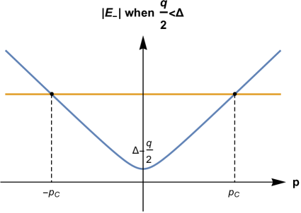
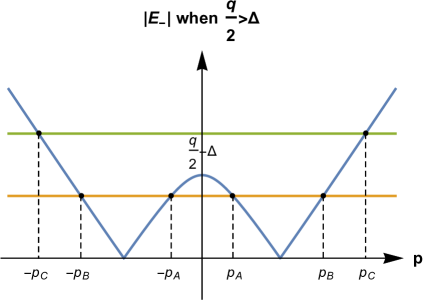
Figure 1: Left: Dispersion relation $E_{-}$ for ${q\over 2}<\Delta$. The horizontal orange line is for $\mu>\Delta-{q\over 2}$. Right: Dispersion relation $E_{-}$ for ${q\over 2}<\Delta$. The horizontal green line is for the case $\mu>{q\over 2}-\Delta$ and the horizontal orange line is for the case $\mu<{q\over 2}-\Delta$. See main text for discussion of the regions of integration in the different cases.

In the limit $T=0$, we can obtain an analytic result for the quark density $n_{q}$ as well. It is given by

$$n_{q} = -{\partial V_{1+}^{\rm med}\over\partial\mu}-{\partial V_{1-}^{\rm med}\over\partial\mu}=2N_{c}\int_{p}\left[\theta(\mu-E_{+})+\theta(\mu-E_{-})\right]$$ (19)

$$= {4N_{c}\over(4\pi)^{2}}\left[{2\over 3}\sqrt{\left(\mu+{q\over 2}\right)^{2}-\Delta^{2}}\left(\mu^{2}-\Delta^{2}+{1\over 4}\mu q-{q^{2}\over 8}\right)+\Delta^{2}q\log{\mu+{q\over 2}+\sqrt{(\mu+{q\over 2})^{2}-\Delta^{2}}\over\Delta}\right]\theta(\mu+\mbox{$q\over 2$}-\Delta)$$

$$+{4N_{c}\over(4\pi)^{2}}\left[{2\over 3}\sqrt{\left(\mu-{q\over 2}\right)^{2}-\Delta^{2}}\left(\mu^{2}-\Delta^{2}-{1\over 4}\mu q-{q^{2}\over 8}\right){\rm sign}(\mu-\mbox{$q\over 2$})-\Delta^{2}q\log{|\mu-{q\over 2}|+\sqrt{(\mu-{q\over 2})^{2}-\Delta^{2}}\over\Delta}\right]$$

$$\times\theta(|\mu-\mbox{$q\over 2$}|-\Delta)\;.$$

The quark density (19) is also independent of the wave vector $q$ when the amplitude $\Delta$ is set to zero, as can be verified by inspection.

III Results and discussion

In the numerical work, we set $N_{c}=3$ everywhere. We use a constituent quark mass $m_{q}=300$ MeV. Since the sigma mass is not very well known experimentally databook , one typically allows it to vary between $m_{\sigma}=400$ MeV and $m_{\sigma}=800$ MeV. We choose $m_{\sigma}=600$ MeV. At the physical point we take $m_{\pi}=140$ MeV and for the pion decay constant we use $f_{\pi}=93$ MeV. In the the chiral limit the pion mass is zero.

It is known from earlier studies in the homogeneous case that vacuum fluctuations play an important role. If we omit the quantum fluctuations, the phase transition in the chiral limit is first order in the entire $\mu$–$T$ plane. If they are included the transition is first order for $T=0$ and second order for $\mu=0$. The first-order line starting on the $\mu$ axis ends at a tricritical point. In the inhomogeneous case, we therefore examine the importance of these fluctuations as well. In Fig. 2, we show the phase diagram in the $\mu$–$T$ plane in the chiral limit without vacuum fluctuations. The solid lines indicate a first-order transition while the dashed line indicates a second-order transition. The region between the two red lines is the inhomogeneous phase. The black line is the first-order transition line in the homogeneous case.

In Fig. 3, we show the phase diagram in the $\mu$–$T$ plane in the chiral limit where vacuum fluctuations are included. The inhomogeneous phase in the entire $\mu$–$T$ plane has now been replaced by a small region at low temperatures. The second-order line starting at $\mu=0$ ends at the Lifshitz point indicated by the full red circle. Since $m_{\sigma}=2m_{q}$ this is also the position of the tricrital point nick2 . The region between the two red lines is the inhomogeneous phase. Comparing Figs. 2 and 3, we see the dramatic effects of including the fermionic vacuum fluctuations.

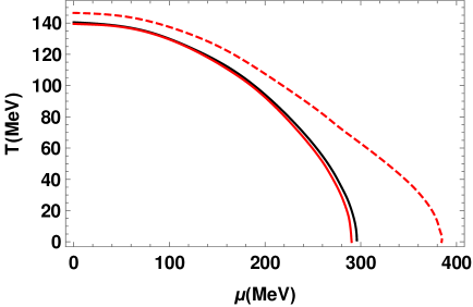
Figure 2: The phase diagram in the $\mu$–$T$ plane for $m_{q}=300$ MeV and $m_{\sigma}=600$ MeV in the chiral limit without quantum fluctuations. A dashed line indicates a second-order transition, while a solid line indicates a first-order transition. The region between the red lines is the inhomogeneous phase.

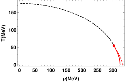
Figure 3: The phase diagram in the $\mu$–$T$ plane for $m_{q}=300$ MeV and $m_{\sigma}=600$ MeV in the chiral limit including vacuum fluctuations. A dashed line indicates a second-order transition, while a solid line indicates a first-order transition. The region between the red lines is the inhomogeneous phase.

Although we find an inhomogeneous phase for finite temperature, it has to be mentioned that this phase might not survive if effects beyond the mean-field approximation are included. There is evidence that in the chiral limit the existence of the Lifshitz point is simply an artifact if the mean-field approximation as pointed out in Ref. japs and Ref. diehl .

In Ref. japs , it is shown that the Goldstone bosons that arise from the breaking of the translational and rotational symmetry have a quadratic dispersion relation in some directions and a linear dispersion relation in other directions. At finite temperature, the former leads to strong long-wavelength fluctuations (phase fluctuations) that destroy off-diagonal long-range order altogether. Long-range order is replaced by quasi-long-range order where the order parameter is decaying algebraically. At $T=0$, the phase fluctuations are not strong enough to destroy this order and there is a true condensate.

In Fig. 4, we show the modulus $\Delta$ (solid blue line) and the wave vector $q$ (dashed red line) as functions of $\mu$ at $T=0$ in the chiral limit with $m_{\sigma}=2m_{q}=600$ MeV. The left panel shows the results without quantum fluctuations and the right panel with. The transition from a phase with homogeneous condensate to a phase with a chiral-density wave is first order, while the transition to a chirally symmetric phase is second order. In the case with no vacuum fluctuations, the vacuum state, i.e. with zero quark density extends all the way to the transition to the CDW phase which extends from $\mu=291\;$MeV up to $\mu=384\;$MeV. This is not the case if we include quantum fluctuations. The vacuum state extends from $\mu=0$ up to $\mu=291$ MeV, where there is a transition to a homogeneous phase with a nonzero quark density and $\Delta$ decreases. This phase extends up to $\mu\approx 322.7$ MeV. In both cases, the vanishing quark density for $\mu<\mu_{c}$, where $\mu_{c}$ is the critical density for the transition to either the CDW phase (left panel) or another homogeneous phase (right panel) with decreasing $\Delta$ is an example of the silver-blaze property. In this phase, all physical quantities are independent of the quark chemical potential cohen .

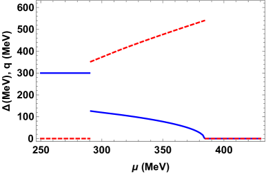
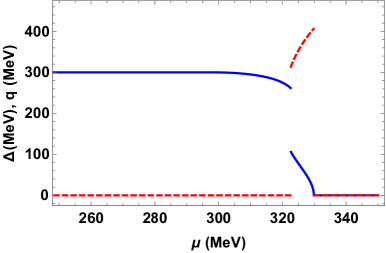
Figure 4: Gap $\Delta$ (solid blue line) and wavevector $q$ (dashed red line) as functions of the quark chemical potential $\mu$ in the chiral limit, at $T=0$, and for $m_{\sigma}=2m_{q}=600$ MeV. Left panel is without vacuum fluctuations and right panel with vacuum fluctuations.

In Fig. 5, we show the modulus $\Delta$ (solid blue line) and the wave vector $q$ (dashed red line) as functions of $\mu$ at $T=0$ at the physical point with $m_{\sigma}=2m_{q}=600$ MeV and $m_{\pi}=140$ MeV. In the left panel, we have omitted the quantum fluctuations and in the right panel, they have been included. Without quantum corrections, there is a transition from a phase with a homogeneous chiral condensate to a phase with a chiral-density wave. This transition is first order. Again, this is in contrast to the case where we include the vacuum fluctuations; the vacuum phase extends from $\mu=0$ to $\mu=300$ MeV and then a second order transition occurs to a phase with a homogeneous quark chiral condensate and a nonzero quark density. In this phase, the chiral condensate decreases. There are two more transitions, one from the phase with a homogeneous chiral condensate (and a nonzero quark density) to a phase with an inhomogeneous phase and a transition to a chirally symmetric phase. Both transitions are first order.

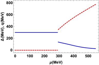
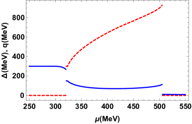
Figure 5: Gap $\Delta$ (solid blue line) and wave vector $q$ (dashed red line) as functions of the quark chemical potential $\mu$ at the physical point for $T=0$ and $m_{\sigma}=2m_{q}=600$ MeV. Left panel is without vacuum fluctuations and right panel with vacuum fluctuations.

The present work can be extended in different directions. For example, it would be of interest to study inhomogeneous phases in a constant magnetic background. Work in this direction is in progress ankn .

Appendix A INTEGRALS AND SUM INTEGRALS

In the imaginary-time formalism for thermal field theory, a fermion has Euclidean 4-momentum $P=(P_{0},{\bf p})$ with $P^{2}=P_{0}^{2}+{\bf p}^{2}$. The Euclidean energy $P_{0}$ has discrete values: $P_{0}=(2n+1)\pi T+i\mu$, where $n$ is an integer. Loop diagrams involve a sum over $P_{0}$ and an integral over spatial momenta $p$. We define the dimensionally regularized sum integral by

$$\hbox{$\sum$}\!\!\!\!\!\!\int_{\{P\}} = T\sum_{P_{0}}\int_{p}\;,$$ (20)

where the integral is in $d=3-2\epsilon$ dimensions

$$\int_{p} = \left({e^{\gamma_{E}}\Lambda^{2}\over 4\pi}\right)^{\epsilon}\int{d^{d}p\over(2\pi)^{d}}$$ (21)

$$= \left({e^{\gamma_{E}}\Lambda^{2}\over 4\pi}\right)^{\epsilon}\int{d^{d-1}p_{\perp}\over(2\pi)^{d-1}}\int{dp_{\parallel}\over 2\pi}$$

$$= \left({e^{\gamma_{E}}\Lambda^{2}\over 4\pi}\right)^{\epsilon}\int{d^{d-1}p_{\perp}\over(2\pi)^{d-1}}{1\over\pi}\int_{\Delta}^{\infty}{u\,du\over\sqrt{u^{2}-\Delta^{2}}}\;.$$

Here $\Lambda$ is the renormalization scale in the modified minimal subtraction scheme $\overline{\rm MS}$, $p_{\parallel}=p_{3}$, $p_{\perp}^{2}=p_{1}^{2}+p_{2}^{2}$ and $u=\sqrt{p_{\parallel}^{2}+\Delta^{2}}$. We need

$$I_{0} = -\hbox{$\sum$}\!\!\!\!\!\!\int_{\{P\}}\log\left[P_{0}^{2}+E^{2}\right]\;.$$ (22)

Summing over the Matsubara frequencies $P_{0}$, we obtain

$$I_{0} = -\int_{p}\bigg{\{}E+T\log\left[1+e^{-\beta(E-\mu)}\right]$$ (23)

$$+T\log\left[1+e^{-\beta(E+\mu)}\right]\bigg{\}}\;.$$

The integral in Eq. (23) is needed for $E=E_{\pm}$ and is calculated by expanding it in powers of $q$, see Appendix C. The integrals that appear are

$$\int_{p}\sqrt{u^{2}+p^{2}_{\perp}} = -{\Delta^{4}\over(4\pi)^{2}}\left({e^{\gamma_{E}}\Lambda^{2}\over\Delta^{2}}\right)^{\epsilon}\Gamma(-2+\epsilon)\;,$$ (24)

$$= -{\Delta^{4}\over 2(4\pi)^{2}}\left({\Lambda^{2}\over\Delta^{2}}\right)^{\epsilon}\left[{1\over\epsilon}+{3\over 2}+{\cal O}(\epsilon)\right]\;,$$

$$\int_{p}{p_{\perp}^{2}\over(u^{2}+p^{2}_{\perp})^{3\over 2}} = -{4\Delta^{2}\over(4\pi)^{2}}\left({e^{\gamma_{E}}\Lambda^{2}\over\Delta^{2}}\right)^{\epsilon}\Gamma(\epsilon)$$ (25)

$$= -{4\Delta^{2}\over(4\pi)^{2}}\left({\Lambda^{2}\over\Delta^{2}}\right)^{\epsilon}\left[{1\over\epsilon}+{\cal O}(\epsilon)\right]\;,$$

$$\int_{p}{p_{\perp}^{2}(4u^{2}-p_{\perp}^{2})\over(u^{2}+p^{2}_{\perp})^{7\over 2}} = -\dfrac{16}{3(4\pi)^{2}}\left({e^{\gamma_{E}}\Lambda^{2}\over\Delta^{2}}\right)^{\epsilon}(-1+\epsilon)\Gamma(1+\epsilon)$$ (26)

$$= {1\over 3\pi^{2}}+\mathcal{O}(\epsilon)\;.$$

We also need some integrals in $D=4-2\epsilon$ dimensions Specifically, we need the integrals

$$A(m^{2}) = \int_{p}{1\over p^{2}-m^{2}}$$ (27)

$$= {im^{2}\over(4\pi)^{2}}\left({\Lambda^{2}\over m^{2}}\right)^{\epsilon}\left[{1\over\epsilon}+1+\mathcal{O}(\epsilon)\right]\;,$$

$$B(p^{2}) = \int_{k}{1\over(k^{2}-m_{q}^{2})[(k+p)^{2}-m_{q}^{2}]}$$ (28)

$$= {i\over(4\pi)^{2}}\left({\Lambda^{2}\over m_{q}^{2}}\right)^{\epsilon}\left[{1\over\epsilon}+F(p^{2})+\mathcal{O}(\epsilon)\right]\;,$$

$$B^{\prime}(p^{2}) = {i\over(4\pi)^{2}}F^{\prime}(p^{2})\;,$$ (29)

where the functions $F(p^{2})$ and $F^{\prime}(p^{2})$ are

$$F(p^{2}) = -\int_{0}^{1}dx\,\log\left[{p^{2}\over m_{q}^{2}}x(x-1)+1\right]$$ (31)

$$= 2-2r\,{\arctan}\left(\mbox{$1\over r$}\right)\;,$$

$$F^{\prime}(p^{2}) = {4m_{q}^{2}r\over p^{2}(4m_{q}^{2}-p^{2})}{\arctan}\left(\mbox{$1\over r$}\right)-{1\over p^{2}}\;,$$ (32)

were we defined $r=\sqrt{{4m_{q}^{2}\over p^{2}}-1}$.

Appendix B PARAMETER FIXING

In this appendix, we find the relation between the parameters in the Lagrangian (1) and the physical observables using the $\overline{\rm MS}$ and OS renormalization schemes.

The sigma and pion self-energies are given by

$$\Sigma_{\sigma}(p^{2}) = -8g^{2}N_{c}\left[A(m_{q}^{2})-\mbox{$1\over 2$}(p^{2}-4m_{q}^{2})B(p^{2})\right]$$ (33)

$$+{4\lambda g\phi_{0}N_{c}m_{q}\over m_{\sigma}^{2}}A(m_{q}^{2})\;,$$

$$\Sigma_{\pi}(p^{2}) = -8g^{2}N_{c}\left[A(m_{q}^{2})-\mbox{$1\over 2$}p^{2}B(p^{2})\right]$$ (34)

$$+{4\lambda g\phi_{0}N_{c}m_{q}\over 3m_{\sigma}^{2}}A(m_{q}^{2})\;,$$

where the last term of Eqs. (33) and (34) is the tadpole contribution to the self-energies, and where the integrals $A(m^{2})$ and $B(p^{2})$ are defined in Eqs. (27) and (28). We do not need the quark self-energy since it is of order $N_{c}^{0}$. Thus $Z_{\psi}=1$ and $\delta m_{q}=0$ at this order. The inverse propagator for the sigma or pion can be written as

$$p^{2}-m_{\sigma,\pi}^{2}-i\Sigma_{\sigma,\pi}(p^{2})+{\rm counterterms}\;.$$ (35)

In the on-shell scheme, the physical mass is equal to the renormalized mass in the Lagrangian. Thus we can write

$$\Sigma_{\sigma,\pi}(p^{2}=m_{\sigma,\pi}^{2}){\rm+counterterms} = 0\;.$$ (36)

The residue of the propagator on shell equals unity, which implies

$${\partial\over\partial p^{2}}\Sigma_{\sigma,\pi}(p^{2})\big{|}_{p^{2}=m_{\sigma,\pi}^{2}}{\rm+counterterms} = 0\;.$$ (37)

The large-$N_{c}$ contribution to the one-point function is

$$\delta\Gamma^{(1)} = -8g^{2}N_{c}\phi_{0}A(m_{q}^{2})+i\delta t\;,$$ (38)

where $\delta t$ is the tadpole counterterm. The equation of motion is equivalent to the vanishing one-point function, which yields on tree level $t=h-m_{\pi}^{2}\phi_{0}=0$. This has to hold also on one-loop level, which gives the renormalization condition

$$\delta\Gamma^{(1)} = 0\;.$$ (39)

The counterterms are given by

$$\Sigma_{\sigma}^{\rm ct1}(p^{2}) = i\left[\delta Z_{\sigma}(p^{2}-m_{\sigma}^{2})-\delta m_{\sigma}^{2}\right]\;,$$ (40)

$$\Sigma_{\pi}^{\rm ct1}(p^{2}) = i\left[\delta Z_{\pi}(p^{2}-m_{\pi}^{2})-\delta m_{\pi}^{2}\right]\;,$$ (41)

$$\Sigma_{\sigma}^{\rm ct2} = 3\Sigma_{\pi}^{\rm ct2}=-{i\lambda\phi_{0}\over m_{\sigma}^{2}}\delta t\;,$$ (42)

$$\delta t = \delta h-f_{\pi}\delta m_{\pi}^{2}-m_{\pi}^{2}\delta f_{\pi}\;,$$ (43)

where the counterterm in Eq. (42) cancels the tadpole contribution to the self-energies. The on-shell renormalization constants are given by the self-energies and their derivatives evaluated at the physical mass. This yields

$$\delta m_{\sigma}^{2} = -i\Sigma_{\sigma}(m_{\sigma}^{2})\;,$$ (44)

$$\delta m_{\pi}^{2} = -i\Sigma_{\pi}(m_{\pi}^{2})\;,$$ (45)

$$\delta Z_{\sigma} = i{\partial\over\partial p^{2}}\Sigma_{\sigma}(p^{2})|_{p^{2}=m_{\sigma}^{2}}\;,$$ (46)

$$\delta Z_{\pi} = i{\partial\over\partial p^{2}}\Sigma_{\pi}(p^{2})|_{p^{2}=m_{\pi}^{2}}\;.$$ (47)

From Eqs. (33)–(38), we find

$$\delta m_{\sigma}^{2} = 8ig^{2}N_{c}\left[A(m_{q}^{2})-\mbox{$1\over 2$}(m_{\sigma}^{2}-4m_{q}^{2})B(m_{\sigma}^{2})\right]\;,$$ (48)

$$\delta m_{\pi}^{2} = 8ig^{2}N_{c}\left[A(m_{q}^{2})-\mbox{$1\over 2$}m_{\pi}^{2}B(m_{\pi}^{2})\right]\;,$$ (49)

$$\delta Z_{\sigma} = 4ig^{2}N_{c}\left[B(m_{\sigma}^{2})+(m_{\sigma}^{2}-4m_{q}^{2})B^{\prime}(m_{\sigma}^{2})\right]\;,$$ (50)

$$\delta Z_{\pi} = 4ig^{2}N_{c}\left[B(m_{\pi}^{2})+m_{\pi}^{2}B^{\prime}(m_{\pi}^{2})\right]\;,$$ (51)

$$\delta t = -8ig^{2}N_{c}f_{\pi}A(m_{q}^{2})\;.$$ (52)

The counterterms $\delta m^{2}$, $\delta\lambda$, $\delta g^{2}$, and $\delta h$ can be expressed in terms of the counterterms $\delta m_{\sigma}^{2}$, $\delta m_{\pi}^{2}$, $\delta Z_{\pi}$, and $\delta t$. Since there is no correction to the quark-pion vertex in the large-$N_{c}$ limit, we find

$$\delta g^{2}=-g^{2}\delta Z_{\pi}\;.$$ (53)

Since there is no correction to the quark mass in the large-$N_{c}$ limit, we find $\delta m_{q}=0$ or

$$\delta g^{2} = -g^{2}{\delta f_{\pi}^{2}\over f_{\pi}^{2}}\;.$$ (54)

This yields $\delta Z_{\pi}={\delta f_{\pi}^{2}\over f_{\pi}^{2}}$. From this relation, Eq. (43), and $h=t+m_{\pi}^{2}f_{\pi}$, one finds

$$\delta m^{2} = -{1\over 2}\left(\delta m_{\sigma}^{2}-3\delta m_{\pi}^{2}\right)\;,$$ (55)

$$\delta\lambda = 3{\delta m_{\sigma}^{2}-\delta m_{\pi}^{2}\over f_{\pi}^{2}}-\lambda\delta Z_{\pi}\;,$$ (56)

$$\delta h = \delta t+f_{\pi}\delta m_{\pi}^{2}+{1\over 2}m_{\pi}^{2}f_{\pi}\delta Z_{\pi}\;.$$ (57)

The expressions for the counterterms are

$$\delta m_{\text{\tiny OS}}^{2} = 8ig^{2}N_{c}\left[A(m_{q}^{2})+\mbox{$1\over 4$}(m_{\sigma}^{2}-4m_{q}^{2})B(m_{\sigma}^{2})-\mbox{$3\over 4$}m_{\pi}^{2}B(m_{\pi}^{2})\right]$$ (58)

$$= \delta m^{2}_{\rm div}+\dfrac{4g^{2}N_{c}}{(4\pi)^{2}}\left\{m^{2}\log\mbox{$\Lambda^{2}\over m_{q}^{2}$}-2m_{q}^{2}-{1\over 2}\left(m_{\sigma}^{2}-4m_{q}^{2}\right)F(m_{\sigma}^{2})+{3\over 2}m_{\pi}^{2}F(m_{\pi}^{2})\right\}\;,$$

$$\delta\lambda_{\text{\tiny OS}} = -\dfrac{12ig^{2}N_{c}}{f_{\pi}^{2}}(m_{\sigma}^{2}-4m_{q}^{2})B(m_{\sigma}^{2})+\dfrac{12ig^{2}N_{c}}{f_{\pi}^{2}}m_{\pi}^{2}B(m_{\pi}^{2})-4i\lambda g^{2}N_{c}\left[B(m_{\pi}^{2})+m_{\pi}^{2}B^{\prime}(m_{\pi}^{2})\right]$$ (59)

$$= \delta\lambda_{\rm div}+\dfrac{12g^{2}N_{c}m_{\sigma}^{2}}{(4\pi)^{2}f_{\pi}^{2}}\left[\left(1-{4m_{q}^{2}\over m_{\sigma}^{2}}\right)\left[\log\mbox{$\Lambda^{2}\over m_{q}^{2}$}+F(m_{\sigma}^{2})\right]+\log\mbox{$\Lambda^{2}\over m_{q}^{2}$}+F(m_{\pi}^{2})+m_{\pi}^{2}F^{\prime}(m_{\pi}^{2})\right]$$

$$-\dfrac{12g^{2}N_{c}m_{\pi}^{2}}{(4\pi)^{2}f_{\pi}^{2}}\left[2\log\mbox{$\Lambda^{2}\over m_{q}^{2}$}+2F(m_{\pi}^{2})+m_{\pi}^{2}F^{\prime}(m_{\pi}^{2})\right]\;,$$

$$\delta g^{2}_{\text{\tiny OS}} = -4ig^{4}N_{c}\left[B(m_{\pi}^{2})+m_{\pi}^{2}B^{\prime}(m_{\pi}^{2})\right]=\delta g_{\rm div}^{2}+\dfrac{4g^{4}N_{c}}{(4\pi)^{2}}\left[\log\mbox{$\Lambda^{2}\over m_{q}^{2}$}+F(m_{\pi}^{2})+m_{\pi}^{2}F^{\prime}(m_{\pi}^{2})\right]\;,$$ (60)

$$\delta h^{\text{\tiny OS}} = -2ig^{2}N_{c}m_{\pi}^{2}f_{\pi}\left[B(m_{\pi}^{2})-m_{\pi}^{2}B^{\prime}(m_{\pi}^{2})\right]$$ (61)

$$= \delta h_{\rm div}+{2g^{2}N_{c}m_{\pi}^{2}f_{\pi}\over(4\pi)^{2}}\left[\log\mbox{$\Lambda^{2}\over m_{q}^{2}$}+F(m_{\pi}^{2})-m_{\pi}^{2}F^{\prime}(m_{\pi}^{2})\right]\;,$$

$$\delta Z_{\sigma}^{\text{\tiny OS}} = \delta Z_{\sigma,\rm div}-\dfrac{4g^{2}N_{c}}{(4\pi)^{2}}\left[\log\mbox{$\Lambda^{2}\over m_{q}^{2}$}+F(m_{\sigma}^{2})+(m_{\sigma}^{2}-4m_{q}^{2})F^{\prime}(m_{\sigma}^{2})\right]\;\;\;,$$ (62)

$$\delta Z_{\pi}^{\text{\tiny OS}} = \delta Z_{\pi,\rm div}-\dfrac{4g^{2}N_{c}}{(4\pi)^{2}}\left[\log\mbox{$\Lambda^{2}\over m_{q}^{2}$}+F(m_{\pi}^{2})+m_{\pi}^{2}F^{\prime}(m_{\pi}^{2})\right]\;,$$ (63)

where $F(m^{2})$ and $F^{\prime}(m^{2})$ are defined in Appendix A, and the divergent quantities are

$$\delta m^{2}_{\rm div} = {4m^{2}g^{2}N_{c}\over(4\pi)^{2}\epsilon}\;,\hskip 28.45274pt\delta\lambda_{\rm div}={8N_{c}\over(4\pi)^{2}\epsilon}\left(\lambda g^{2}-6g^{4}\right)\;,\hskip 28.45274pt\delta g_{\rm div}^{2}={4g^{4}N_{c}\over(4\pi)^{2}\epsilon}\;,$$ (64)

$$\delta Z_{\sigma,\rm div} = \delta Z_{\pi,\rm div}=-{4g^{2}N_{c}\over(4\pi)^{2}\epsilon}\;,\hskip 28.45274pt\delta h_{\rm div}{2g^{2}hN_{c}\over(4\pi)^{2}\epsilon}\;.$$ (65)

The divergent parts of the counterterms are the same in the two schemes, i.e. $\delta m^{2}_{\rm div}=\delta m^{2}_{\overline{\text{\tiny MS}}}$ and so forth. Since the bare parameters are independent of the renormalization scheme, we can immediately write down relations between the renormalized parameters in the on-shell and $\overline{\rm MS}$ schemes. We find

$$m^{2}_{\overline{\text{\tiny MS}}} = m^{2}+\delta m^{2}_{\text{\tiny OS}}-\delta m^{2}_{\overline{\text{\tiny MS}}}$$ (66)

$$\lambda_{\overline{\text{\tiny MS}}} = \lambda+\delta\lambda_{\text{\tiny OS}}-\delta\lambda_{\overline{\text{\tiny MS}}}$$ (67)

$$g_{\overline{\text{\tiny MS}}}^{2} = g^{2}+\delta g^{2}_{\text{\tiny OS}}-\delta g^{2}_{\overline{\text{\tiny MS}}}\;,$$ (68)

$$h_{\overline{\text{\tiny MS}}} = h+\delta h_{\text{\tiny OS}}-\delta h_{\overline{\text{\tiny MS}}}\;.$$ (69)

Using Eqs. (58)–(61), we find the running parameters in the $\overline{\rm MS}$ scheme

$$m^{2}_{\overline{\text{\tiny MS}}} = m^{2}+8ig^{2}N_{c}\left[A(m_{q}^{2})+\mbox{$1\over 4$}(m_{\sigma}^{2}-4m_{q}^{2})B(m_{\sigma}^{2})-\mbox{$3\over 4$}m_{\pi}^{2}B(m_{\pi}^{2})\right]-\delta m^{2}_{\overline{\text{\tiny MS}}}$$ (70)

$$= m^{2}+\dfrac{4g^{2}N_{c}}{(4\pi)^{2}}\left[m^{2}\log\mbox{$\Lambda^{2}\over m_{q}^{2}$}-2m_{q}^{2}-{1\over 2}\left(m_{\sigma}^{2}-4m_{q}^{2}\right)F(m_{\sigma}^{2})+{3\over 2}{m_{\pi}^{2}}F(m_{\pi}^{2})\right]\;,$$

$$\lambda_{\overline{\text{\tiny MS}}} = \lambda-\dfrac{12ig^{2}N_{c}}{f_{\pi}^{2}}(m_{\sigma}^{2}-4m_{q}^{2})B(m_{\sigma}^{2})+\dfrac{12ig^{2}N_{c}}{f_{\pi}^{2}}m_{\pi}^{2}B(m_{\pi}^{2})-4i\lambda g^{2}N_{c}\left[B(m_{\pi}^{2})+m_{\pi}^{2}B^{\prime}(m_{\pi}^{2})\right]-\delta\lambda_{\overline{\text{\tiny MS}}}$$ (71)

$$= \lambda+\bigg{\{}\dfrac{12g^{2}N_{c}}{(4\pi)^{2}f_{\pi}^{2}}\left[(m_{\sigma}^{2}-4m_{q}^{2})\left(\log\mbox{$\Lambda^{2}\over m_{q}^{2}$}+F(m_{\sigma}^{2})\right)+m_{\sigma}^{2}\left(\log\mbox{$\Lambda^{2}\over m_{q}^{2}$}+F(m_{\pi}^{2})+m_{\pi}^{2}F^{\prime}(m_{\pi}^{2})\right)\right.$$

$$\left.-m_{\pi}^{2}\left(2\log\mbox{$\Lambda^{2}\over m_{q}^{2}$}+2F(m_{\pi}^{2})+F^{\prime}(m_{\pi}^{2})\right)\right]\bigg{\}}\;,$$

$$g_{\overline{\text{\tiny MS}}}^{2} = g^{2}-4ig^{4}N_{c}\left[B(m_{\pi}^{2})+m_{\pi}^{2}B^{\prime}(m_{\pi}^{2})\right]-\delta g_{\overline{\text{\tiny MS}}}^{2}$$ (72)

$$= g^{2}\left\{1+\dfrac{4g^{2}N_{c}}{(4\pi)^{2}}\left[\log\mbox{$\Lambda^{2}\over m_{q}^{2}$}+F(m_{\pi}^{2})+m_{\pi}^{2}F^{\prime}(m_{\pi}^{2})\right]\right\}\;,$$

$$h_{\overline{\text{\tiny MS}}} = h-2ig^{2}N_{c}h\left[B(m_{\pi}^{2})-m_{\pi}^{2}B^{\prime}(m_{\pi}^{2})\right]-\delta h_{\overline{\text{\tiny MS}}}$$ (73)

$$= h+{2g^{2}N_{c}h\over(4\pi)^{2}}\left[\log\mbox{$\Lambda^{2}\over m_{q}^{2}$}+F(m_{\pi}^{2})-m_{\pi}^{2}F^{\prime}(m_{\pi}^{2})\right]\;,$$

where the physical on-shell values are related to the meson and quark masses given by Eqs. (4)–(5).

Appendix C EFFECTIVE POTENTIAL

In this appendix, we calculate the one-loop effective potential in the $\overline{\rm MS}$ scheme. It reads

$$V_{1} = -2N_{c}\hbox{$\sum$}\!\!\!\!\!\!\int_{\{P\}}\log[P_{0}^{2}+E_{\pm}^{2}]$$ (74)

$$= -2N_{c}\int_{p}\bigg{\{}E_{\pm}+T\log\left[1+e^{-\beta(E_{\pm}-\mu)}\right]$$

$$+T\log\left[1+e^{-\beta(E_{\pm}+\mu)}\right]\bigg{\}}\;,$$

where the sum integral is defined in Eq. (20). The vacuum integrals needed are

$$V_{\pm} = -2N_{c}\int_{p}E_{\pm}\;.$$ (75)

We first integrate over angles in the $(p_{1},p_{2})$ plane and introduce the variable $u=\sqrt{p_{\parallel}^{2}+\Delta^{2}}$. The expression for $V_{\pm}$ can then be written as

$$V_{\pm} = -{16N_{c}(e^{\gamma_{E}}\Lambda^{2})^{\epsilon}\over(4\pi)^{2}\Gamma(1-\epsilon)}\int_{\Delta}^{\infty}{u\,du\over\sqrt{u^{2}-\Delta^{2}}}$$ (76)

$$\times\int_{0}^{\infty}\sqrt{\left(u\pm{q\over 2}\right)^{2}+p_{\perp}^{2}}\,p_{\perp}^{1-2\epsilon}dp_{\perp}\;.$$

The strategy is to isolate the ultraviolet divergences in Eq. (76) by expanding the integrand and identifying appropriate subtraction terms ${\rm sub}_{\pm}(u,p_{\perp})$. The integral of the subtraction terms can be done in dimensional regularization, while the integral of $E_{\pm}-{\rm sub}_{\pm}(u,p_{\perp})$ is finite and can be calculated directly in three dimensions. The subtraction term ${\rm sub}_{\pm}(u,p_{\perp})$ is found by expanding Eq. (76) through order $q^{4}$. This yields

$${\rm sub}_{\pm}(u,p_{\perp}) = \sqrt{u^{2}+p^{2}_{\perp}}\pm{uq\over 2\sqrt{u^{2}+p_{\perp}^{2}}}+{q^{2}p_{\perp}^{2}\over 8(u^{2}+p_{\perp}^{2})^{3\over 2}}\mp{q^{3}p_{\perp}^{2}u\over 16(u^{2}+p_{\perp}^{2})^{5\over 2}}+{q^{4}p_{\perp}^{2}(4u^{2}-p_{\perp}^{2})\over 128(u^{2}+p_{\perp}^{2})^{7\over 2}}\;.$$ (77)

We write the integrals in (76) as

$$V_{\pm} = V_{\rm div\pm}+V_{\rm fin\pm}\;,$$ (78)

where

$$V_{\rm div\pm} = -{16N_{c}(e^{\gamma_{E}}\Lambda^{2})^{\epsilon}\over(4\pi)^{2}\Gamma(1-\epsilon)}\int_{\Delta}^{\infty}{u\,du\over\sqrt{u^{2}-\Delta^{2}}}\int_{0}^{\infty}{\rm sub}_{\pm}(u,p_{\perp})p_{\perp}^{1-2\epsilon}\,dp_{\perp}\;,$$ (79)

$$V_{\rm fin\pm} = -{16N_{c}(e^{\gamma_{E}}\Lambda^{2})^{\epsilon}\over(4\pi)^{2}\Gamma(1-\epsilon)}\int_{\Delta}^{\infty}{u\,du\over\sqrt{u^{2}-\Delta^{2}}}\int_{0}^{\infty}\left[\sqrt{\left(u\pm{q\over 2}\right)^{2}+p_{\perp}^{2}}-{\rm sub}_{\pm}(u,p_{\perp})\right]p_{\perp}^{1-2\epsilon}\,dp_{\perp}\;.$$ (80)

The integral $V_{\rm fin\pm}$ can now be calculated directly in three dimensions. After integrating over $p_{\perp}$, we find

$$V_{\rm fin\pm} = -{16N_{c}\over 3(4\pi)^{2}}\int_{\Delta}^{\infty}(u\pm\mbox{$q\over 2$})^{2}\left[\left(u\pm\mbox{$q\over 2$}\right)-\big{|}u\pm\mbox{$q\over{2}$}\big{|}\right]{u\,du\over\sqrt{u^{2}-\Delta^{2}}}\;.$$ (81)

Thus $V_{\rm fin+}$ vanishes identically and $V_{\rm fin-}$ becomes

$$V_{\rm fin-} = -{32N_{c}\over 3(4\pi)2^{2}}\int_{\Delta}^{\infty}(u-\mbox{$q\over 2$})^{3}\theta(\mbox{$q\over 2$}-\Delta){u\,du\over\sqrt{u^{2}-\Delta^{2}}}$$ (82)

$$= {N_{c}\over 3(4\pi)^{2}}\left[q\sqrt{{q^{2}\over 4}-\Delta^{2}}(26\Delta^{2}+q^{2})-12\Delta^{2}(\Delta^{2}+q^{2})\log{{q\over 2}+\sqrt{{q^{2}\over 4}-\Delta^{2}}\over\Delta}\right]\theta(\mbox{$q\over 2$}-\Delta)\;.$$

We next integrate $V_{\rm div\pm}$ using dimensional regularization. Again this is done by first integrating over $p_{\perp}$ and then over $u$. This yields

$$V_{\rm div} = V_{\rm div+}+V_{\rm div-}$$ (83)

$$= {2N_{c}\over(4\pi)^{2}}\left({e^{\gamma_{E}}\Lambda^{2}\over\Delta^{2}}\right)^{\epsilon}\left[2\Delta^{4}\Gamma(-2+\epsilon)+q^{2}\Delta^{2}\Gamma(\epsilon)+{q^{4}\over 12}(-1+\epsilon)\Gamma(1+\epsilon)\right]\;.$$

Expanding Eq. (83) to zeroth order in powers of $\epsilon$, we obtain

$$V_{\rm div} = {2N_{c}\over(4\pi)^{2}}\left({\Lambda^{2}\over\Delta^{2}}\right)^{\epsilon}\left[\left({1\over\epsilon}+{3\over 2}\right)\Delta^{4}+{1\over\epsilon}\Delta^{2}q^{2}-{q^{4}\over 12}+{\cal O}(\epsilon)\right]\;.$$ (84)

The one-loop effective potential is then given by the sum of Eqs. (82) and (84). It contains poles in $\epsilon$, which are removed by mass and coupling-constant renormalization. In the $\overline{\rm MS}$ scheme, this amounts to making the substitutions $m^{2}\rightarrow Z_{m^{2}}m^{2}$, $\lambda\rightarrow Z_{\lambda}\lambda$, $g^{2}\rightarrow Z_{g^{2}}g^{2}$, and $h\rightarrow Z_{h}h$, where

$$Z_{m^{2}}=1+{4N_{c}g^{2}\over(4\pi)^{2}\epsilon}\;,\hskip 22.76228ptZ_{\lambda}=1+{8N_{c}\over(4\pi)^{2}\epsilon}\left[\lambda g^{2}-6g^{4}\right]\;,\hskip 22.76228ptZ_{g^{2}}=1+{4N_{c}g^{2}\over(4\pi)^{2}\epsilon}\hskip 22.76228ptZ_{h}=1+{2N_{c}g^{2}\over(4\pi)^{2}\epsilon}\;.$$ (85)

After renormalization, the vacuum energy in the mean-field approximation reads

$$V_{+}+V_{-} = {1\over 2}{q^{2}\over g_{\overline{\text{\tiny MS}}}^{2}(\Lambda^{2})}\Delta^{2}+{1\over 2}{m_{\overline{\text{\tiny MS}}}^{2}(\Lambda^{2})\over g_{\overline{\text{\tiny MS}}}^{2}(\Lambda^{2})}\Delta^{2}+{\lambda_{\overline{\text{\tiny MS}}}(\Lambda^{2})\over 24g_{\overline{\text{\tiny MS}}}^{4}(\Lambda^{2})}\Delta^{4}-{h_{\overline{\text{\tiny MS}}}(\Lambda^{2})\over g_{\overline{\text{\tiny MS}}}(\Lambda^{2})}\Delta+{2N_{c}\Delta^{2}q^{2}\over(4\pi)^{2}}\log{\Lambda^{2}\over\Delta^{2}}+{2N_{c}\Delta^{4}\over(4\pi)^{2}}\left[\log{\Lambda^{2}\over\Delta^{2}}+{3\over 2}\right]$$ (86)

$$-{N_{c}q^{4}\over 6(4\pi)^{2}}+{N_{c}\over 3(4\pi)^{2}}\left[q\sqrt{{q^{2}\over 4}-\Delta^{2}}(26\Delta^{2}+q^{2})-12\Delta^{2}(\Delta^{2}+q^{2})\log{{q\over 2}+\sqrt{{q^{2}\over 4}-\Delta^{2}}\over\Delta}\right]\theta(\mbox{$q\over 2$}-\Delta)\;,$$

where the argument $\Lambda$ indicates that the renormalized parameters are running and the subscript $\overline{\text{\tiny MS}}$ indicates the scheme. They satisfy the following renormalization group equations:

$$\Lambda{dm_{\overline{\text{\tiny MS}}}^{2}(\Lambda)\over d\Lambda} = {8N_{c}m^{2}_{\overline{\text{\tiny MS}}}(\Lambda)g_{\overline{\text{\tiny MS}}}^{2}(\Lambda)\over(4\pi)^{2}}\;,$$ (87)

$$\Lambda{dg_{\overline{\text{\tiny MS}}}^{2}(\Lambda)\over d\Lambda} = {8N_{c}g_{\overline{\text{\tiny MS}}}^{4}(\Lambda)\over(4\pi)^{2}}\;,$$ (88)

$$\Lambda{d\lambda_{\overline{\text{\tiny MS}}}(\Lambda)\over d\Lambda} = {16N_{c}\over(4\pi)^{2}}\left[\lambda_{\overline{\text{\tiny MS}}}(\Lambda)g^{2}_{\overline{\text{\tiny MS}}}(\Lambda)-6g^{4}_{\overline{\text{\tiny MS}}}(\Lambda)\right]\;,$$ (89)

$$\Lambda{dh_{\overline{\text{\tiny MS}}}(\Lambda)\over d\Lambda} = {4N_{c}g^{2}_{\overline{\text{\tiny MS}}}(\Lambda)h_{\overline{\text{\tiny MS}}}(\Lambda)\over(4\pi)^{2}}\;.$$ (90)

The solutions to Eqs. (87)–(90) are

$$m_{\overline{\text{\tiny MS}}}^{2}(\Lambda) = {m_{0}^{2}\over 1-{4g_{0}^{2}N_{c}\over(4\pi)^{2}}\log{\Lambda^{2}\over\Lambda_{0}^{2}}}\;,$$ (91)

$$g_{\overline{\text{\tiny MS}}}^{2}(\Lambda) = {g_{0}^{2}\over 1-{4g_{0}^{2}N_{c}\over(4\pi)^{2}}\log{\Lambda^{2}\over\Lambda_{0}^{2}}}\;,$$ (92)

$$\lambda_{\overline{\text{\tiny MS}}}(\Lambda) = {\lambda_{0}-{48g_{0}^{4}N_{c}\over(4\pi)^{2}}\log{\Lambda^{2}\over\Lambda_{0}^{2}}\over\left(1-{4g_{0}^{2}N_{c}\over(4\pi)^{2}}\log{\Lambda^{2}\over\Lambda_{0}^{2}}\right)^{2}}\;,$$ (93)

$$h_{\overline{\text{\tiny MS}}}(\Lambda) = {h_{0}\over 1-{2g_{0}^{2}N_{c}\over(4\pi)^{2}}\log{\Lambda^{2}\over\Lambda_{0}^{2}}}\;,$$ (94)

The parameters $m_{0}^{2}$, $g_{0}^{2}$, $\lambda_{0}$ and $h_{0}$, are the values of the running parameters at the scale $\Lambda_{0}$, where we choose $\Lambda_{0}$ to satisfy

$$\log{\Lambda_{0}^{2}\over m_{q}^{2}}+F(m_{\pi}^{2})+m_{\pi}^{2}F^{\prime}(m_{\pi}^{2}) = 0\;.$$ (95)

$F(m_{\pi}^{2})$ and $m_{\pi}^{2}F^{\prime}(m_{\pi}^{2})$ vanish in the chiral limit which implies that $\Lambda_{0}=m_{q}$. We can now evaluate Eqs. (70)–(73) at $\Lambda=\Lambda_{0}$ to find $m_{0}^{2}$, $\lambda_{0}$, $g_{0}^{2}$, and $h_{0}$. Inserting Eqs. (91)–(94) into Eq. (86) using the results for $m_{0}^{2}$, $\lambda_{0}$, $g_{0}^{2}$, and $h_{0}$, we obtain the final result Eq. (7).

References

- (1) Y. Aoki, Z. Fodor, S. Katz, and K. Szabo, Phys. Lett. B 643, 46 (2006),
- (2) Y. Aoki, S. Borsanyi, S. Durr, Z. Fodor, S.D. Katz et al., JHEP 0906, 088 (2009),
- (3) S. Borsanyi et al. (Wuppertal-Budapest Collaboration), JHEP 1009, 073 (2010)
- (4) A. Bazavov, T. Bhattacharya, M. Cheng, C. DeTar, H. Ding et al., Phys.Rev. D 85, 054503 (2012).
- (5) J. Casalderrey-Solana, H. Liu, D. Mateos, K. Rajagopal, and U. A. Wiedemann, Gauge/String Duality, Hot QCD and Heavy Ion Collisions. Cambridge University Press, (2014).
- (6) S. Mogliacci, J. O. Andersen, M. Strickland, N. Su, A. Vuorinen, JHEP 1312, 055 (2013).
- (7) N. Haque, A. Bandyopadhyay, J. O. Andersen, M. G. Mustafa, M. Strickland, and N. Su, JHEP 1405, 027 (2014).
- (8) M. G. Alford, A. Schmitt, and K. Rajagopal, Rev. Mod. Phys. 80, 1455 (2008).
- (9) C. Itzykson, and J.-B. Zuber, Quantum Field Theory, 540, McGraw-Hill (1980).
- (10) M. Gell-Mann, and M. Lévy, Nuovo Cim 16, 705, (1960).
- (11) K. Fukushima, Phys. Lett. B 591, 277 (2004).
- (12) K. Fukushima, and T. Hatsuda, Rept. Prog. Phys. 74, 014001 (2011).
- (13) R. Anglani, R. Casalbuoni, M. Ciminale, N. Ippolito, R. Gatto, M. Mannarelli, and M. Ruggieri, Rev. Mod. Phys. 86, 509 (2014).
- (14) M. Buballa and S. Carignano, Prog. Part. Nucl. Phys. 81, 39 (2015).
- (15) T. Kojo, Y. Hidaka, L. McLerran, and R. D. Pisarski, Nucl. Phys. A 843, 37 (2010); ibid 875, 94, (2011).
- (16) D. Nickel, Phys. Rev. Lett. 103, 072301 (2009).
- (17) H. Abuki and D. Ishibashi, Phys. Rev. D 85, 074002 (2012).
- (18) T.-G. Lee, E. Nakano, Y. Tsue, T. Tatsumi, B. Friman, Phys. Rev. D 92, 034024 (2015).
- (19) Y. Hidaka, K. Kamikado, T. Kanazawa, and T. Noumi, Phys. Rev. D 92, 034003 (2015).
- (20) E. Nakano and T. Tatsumi, Phys. Rev. D 71, 114006 (2005).
- (21) S. Maedan, Prog. Theor. Phys. 123, 285 (2010).
- (22) D. Nickel, Phys. Rev. D 80, 074025 (2009).
- (23) S. Karasawa and T. Tatsumi, Phys. Rev. D 92, 116004 (2015).
- (24) A. Heinz, F. Giacosa, M. Wagner, and D. H. Rischke, Phys. Rev. D 93, 014007 (2016).
- (25) R. Yoshiike, T.-G. Lee, and T. Tatsumi, e-Print: arXiv:1702.01511 [hep-ph].
- (26) S. Carignano, D. Nickel, and M. Buballa, Phys. Rev. D 82, 054009 (2010).
- (27) J. Braun, F. Karbstein, S. Rechenberger, and D. Roscher Phys. Rev. D 93, 014032 (2016).
- (28) S. Carignano, M. Buballa, and B.-J. Schaefer, Phys. Rev. D 90, 014033 (2014).
- (29) S. Carignano, M. Buballa, and W. Elkamhawy, Phys. Rev. D 94, 034023 (2016).
- (30) J. P. Carlomagno, D. Gomez Dumm, and N. N. Scoccola, Phys. Rev. D 92, 056007 (2015).
- (31) P. de Forcrand and U. Wenger,PoS LAT2006, 152 (2006).
- (32) M. Wagner, Phys. Rev. D 76, 076002 (2007).
- (33) F. Dautry and E. M. Nyman, Nucl. Phys. A 319, 323 (1979).
- (34) P. Adhikari, J. O. Andersen, and P. Kneschke, Phys. Rev. D 95, 036017 (2017).
- (35) P. Adhikari and J. O. Andersen, Phys. Rev. D 95, 036009 (2017).
- (36) D. Ebert, N. V. Gubina, K. G. Klimenko, S. G. Kurbanov, and V. Ch. Zhukovsky, Phys. Rev. D 84, 025004 (2011).
- (37) Particle data group, http://pdg.lbl.gov/2014/listings/rpp2014-list-f0-500.pdf.
- (38) T. D. Cohen, Phys. Rev. Lett. 91, 222001 (2003).
- (39) H. W. Diehl, Acta physica slovaca 52 (4), 271 (2002).
- (40) J. O. Andersen, and P. Kneschke, in preparation (2017)