Assessing of a portion of the Pacific Thunnus albacares stock:
Ahi in the Main Hawaiian Islands

Abstract

Regional tuna fishery management organizations cannot provide specific advice to local fishery managers in small island jurisdictions. The State of Hawaii maintains time series of yellowfin tuna catches dating back to 1949, but these data have never been formally applied to evaluating the effects of the yellowfin fishery in the Main Hawaiian Islands on the local stock. I develop a new approach utilizing these data that links the local stock dynamics to the dynamics of the larger Pacific stock. This approach uses a state-space logistic production model linked to the larger Pacific stock using an index of abundance. The conclusion is that such a model is feasible, that the local stock is not overfished and that local fisheries are fishing at acceptable levels.

Introduction

The responsibility to manage fisheries for tunas and tuna-like species usually lies with regional organizations established under international treaties. In the Western Central Pacific Ocean (WCPO), this responsibility devolves to the Western and Central Pacific Fisheries Commission (WCPFC, https://www.wcpfc.int). The WCPFC conducts stock assessments for several species of tunas and implements fishery management and conservation measures based on these stock assessments. These WCPFC stock assessments and conservation and management measures may assist the WCPFC in regulating large scale fisheries in the stock habitat, but offer little useful advice to managers of small scale fisheries operating outside of the primary equatorial fishing grounds.

Yellowfin tuna (Thunnus albacares, YFT) is an important food resource of many Pacific Island communities and the people of the Hawaiian islands of been fishing for yellowfin for many generations. Recent studies (Rooker et al. 2016) have shown that the Hawaii-based fishery for YFT is supported by local production with little or no subsidies from equatorial production zones or nurseries. The Main Hawaiian Islands (MHI), Figure 1, comprising the 8 largest islands in the Hawaiian Archipelago, have been important fishing grounds throughout this history. Since the recent expansion of the Papahānaumokuākea Marine National Monument in 2016, the MHI is the only legally accessible tuna fishing ground in the State of Hawaii. This change emphasizes the importance of careful management of yellowfin fisheries in the MHI.

Figure 1: The United States Exclusive Economic Zone around the Hawaiian Archipelago. The Main Hawaiian Islands lie in the shaded area at the extreme east of the EEZ. The line at 20^∘N latitude is the boundary between WCPFC stock assessment regions 2 and 4. See text for full explanation.

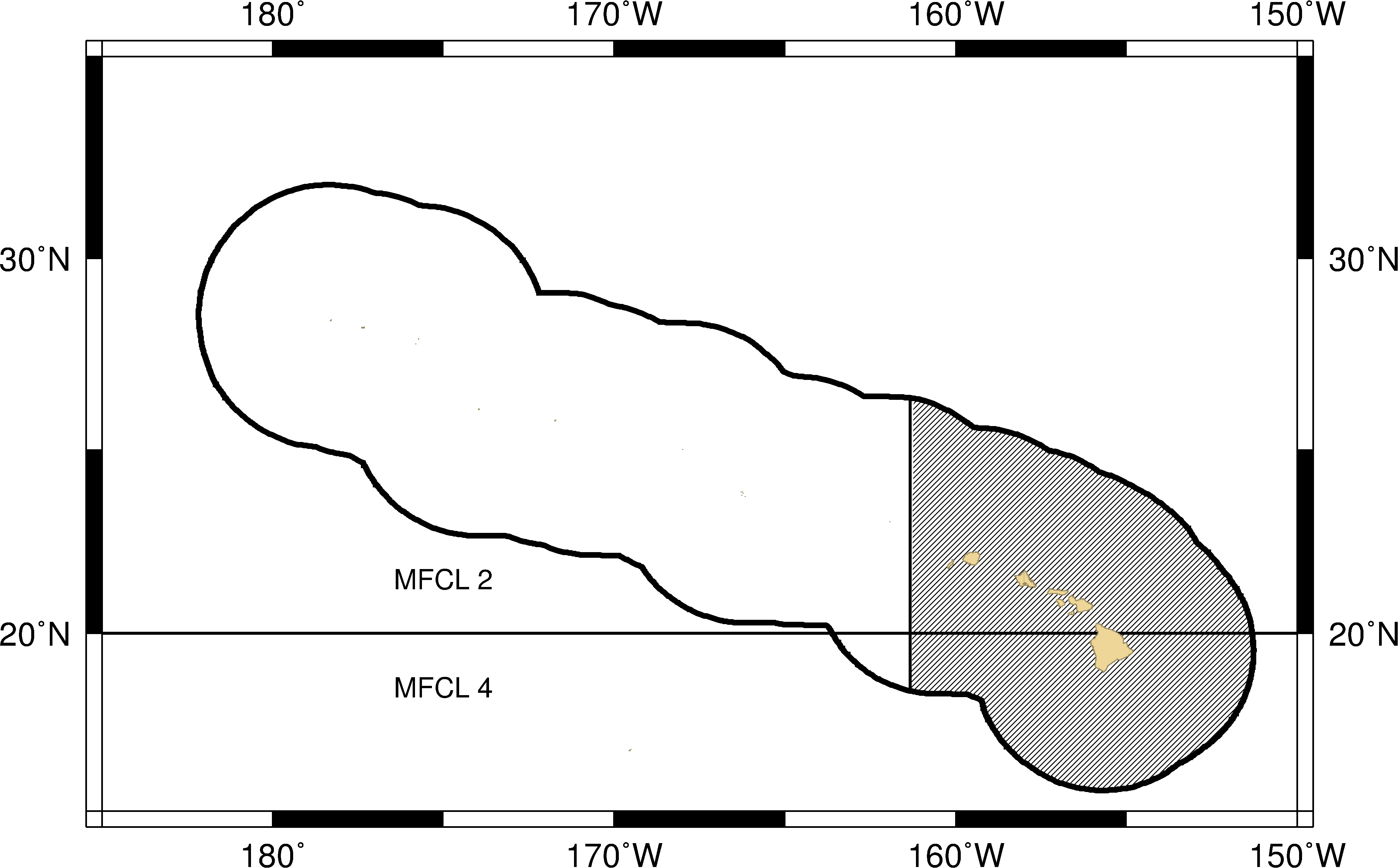
The primary purpose of this paper is to explore a means to apply the 65 year time series of data collected from local fisheries to the problem of providing advice to fisheries managers about the effects of local fisheries on the local portion of the larger stock of yellowfin tuna in the Pacific. The general approach is to develop a relatively simple population dynamics model, estimate the model parameters from existing data, and apply the estimated parameters to answer the question of the effects of the fishery. I adopt a state-space variant of the logistic surplus production model with several novel features. Fishing mortality, the proportion of the population harvested each year, is represented as a random walk of multiple gear types. Offline coupling is used to link the local biomass to regional biomass estimates by large scale yellowfin stock assessment models developed for the WCPFC. The logistic parameters of the surplus production model are reparameterized to estimate parameters of direct relevance to fishery management. All state transitions are represented as random effects.

Methods

State-space models separate variability in the biological processes in the system (transition model) from errors in observing features of interest in the system (observation model).

The general form of the transition model is

$$\alpha_{t}=T(\alpha_{t-1})+\eta_{t}$$ (1)

where $\alpha_{t}$ is the state at time $t$ and the function $T$ embodies the dynamics mediating the development of the state at time $t$ from the state at the previous time with random process error, $\eta_{t}$.

Stock dynamics follow the classic Schaefer (1954) differential equation:

$$\frac{dN}{dt}=rN(1-\frac{N}{K})-FN$$ (2)

where $N$ is the biomass of YFT in the MHI (measured in metric tonnes, mt), $r$ is the logistic growth rate (yr^-1), $K$ is the asymptotic biomass (mt), and $F$ is the total fishing mortality (yr^-1) in the MHI.

The state space transition equation is developed by solving (2) analytically from one time to the next and applying a random error.

$$N_{t}=\frac{K(r-\bar{F}_{t})}{\frac{K(r-\bar{F}_{t})}{N_{t-\Delta t}}e^{-\Delta t(r-\bar{F}_{t})}-re^{-\Delta t(r-\bar{F}_{t})}-r}\cdot e^{\eta_{t}};\quad\eta_{t}\sim N(0,\sigma^{2}_{N})$$ (3)

where $\eta_{t}\sim N(0,\sigma_{N})$ is a process error expressing variability in population dynamics and $\bar{F}_{t}$ is the total fishing mortality exerted by all gears, i. e.,

$$\bar{F}_{t}=\sum_{g=1}^{n}F_{g,t}.$$ (4)

The logarithm of fishing mortality for each gear is assumed to follow a random walk with normal increments, as suggested by Nielsen and Berg (2014).

$$\log F_{g,t}=\log F_{g,t-1}+\xi_{t};\quad\xi_{t}\sim N(0,\sigma^{2}_{F})$$ (5)

where $\xi_{t}$ is a process error expressing the year to year variability in fishing mortality.

An index of abundance assumes that the biomass of YFT in the MHI is approximately proportional to some index which is independent of the data analyzed in the model,

$$\log N_{t}-\log(Q\cdot I_{t})=\omega_{t};\quad\omega_{t}\sim N(0,\sigma^{2}_{I})$$ (6)

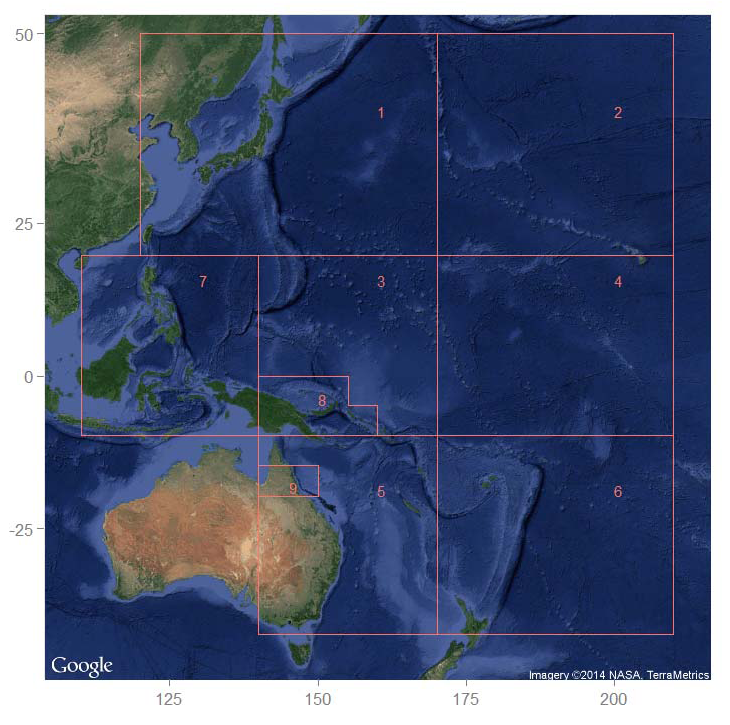
where $I_{t}$ is the index (mt) at time $t$, $Q$ is the estimated ratio of the MHI population size to the index, and $\omega_{t}$ is a process error representing the difference between the MHI biomass and the abundance index. Conventional fishery independent methods, such as acoustic or trawl surveys, are not available for tunas. Biomass estimates from the most recent WCPFC stock assessment (Davies, et al. 2014) are convenient potential abundance indices. The assessment method used by the WCPFC is spatially structured and estimates biomass in several regions in the Pacific Ocean. The boundary between regions 2 and 4 passes directly through the MHI (Figure 1). Biomass estimates from both regions were evaluated as abundance indices.

The logistic parameters $r$ and $K$ are notoriously difficult to estimate in surplus production models, so parameter substitutions were used. Maximum sustainable yield (MSY, $\widetilde{Y}$) and fishing mortality at MSY ($F_{\widetilde{Y}}$) are commonly used fishery reference points and are simple functions of $r$ and $K$. Therefore $\widetilde{Y}$ and $F_{\widetilde{Y}}$ were estimated directly and substituted in (3) as $r=2F_{\widetilde{Y}}$ and $K=\frac{4\widetilde{Y}}{r}$.

Carruthers and McAllister (2011) recommend use of Bayesian priors for the logistic growth parameter, $r$, in equation (2). They suggest $\tilde{r}=0.486$ with a standard deviation of $\sigma_{r}=0.046$ (a coefficient of variation ${\rm cv}=\frac{\sigma_{r}}{r}=0.094$) for Atlantic YFT. A lognormal prior on $r$ was implemented as

$$\log r-\log\tilde{r}=\rho;\quad\rho\sim N(0,\sigma^{2}_{r});$$ (7)

$\rho$ becomes a component of the likelihood (equation 11).

This model assumes three Normal $N(0,\sigma^{2})$ process errors with standard deviations, $\sigma_{N}$, $\sigma_{I}$, and $\sigma_{F}$. The first two, $\sigma_{N}$ and $\sigma_{I}$, pertain to the evolution of biomass over time. It is assumed that these two standard deviations can be represented by a single parameter, $\sigma_{P}$. The third standard deviation, $\sigma_{F}$, pertains to the fishing mortality.

The general form of the state space observation model is

$$x_{t}=O(\alpha_{t})+\varepsilon_{t}$$ (8)

where the function $O$ describes the measurement process with error $\varepsilon$ in observing the state.

Predicted catch, $\widehat{C}_{g,t}$, for each gear is the product of estimated fishing mortality and the biomass,

$$\widehat{C}_{g,t}=F_{g,t}\cdot\Bigl{(}\frac{N_{t-\Delta t}+N_{t}}{2}\Bigr{)}\cdot e^{\varepsilon_{t}}$$ (9)

where the biomass is the average biomass over the time step (Quinn and Deriso, 1999), and $\varepsilon_{t}$ is a “zero-inflated” log normal likelihood given by

$$\log\varepsilon_{t}=\left\{\begin{array}[]{r@{\;:\quad}l}C_{g,t}>0&(1-p_{0})\cdot\bigg{(}\log\frac{1}{\sqrt{2\pi\sigma^{2}_{Y}}}-\Bigl{(}\frac{\log C_{g,t}-\log\widehat{C}_{g,t}}{\sigma_{Y}}\Bigr{)}^{2}\bigg{)}\\ C_{g,t}=0&p_{0}\cdot\log\frac{1}{\sqrt{2\pi\sigma^{2}_{Y}}}\\ \end{array}\right.$$ (10)

where $C_{g,t}$ is the observed catch for gear $g$ at time $t$, $\sigma_{Y}$ is the observation error and $p_{0}$ is the proportion of observed catch observations equal to zero.

Table 1: Complete list of estimated and computed parameters and model constraints for the state-space surplus production model. There are 6 estimated parameters. The three computed variables are functions of estimated parameters. There are four constraints and constants. For a model with 61 time steps and 4 gear types, there are 305 random effects.

Parameter	Definition
	Estimated parameters:
$\widetilde{Y}$	Maximum sustainable yield (mt).
$F_{\widetilde{Y}}$	Fishing mortality at maximum sustainable yield (yr-1).
$Q$	Abundance index proportionality constant
$\sigma_{P}$	Biomass random walk process error standard deviation,
	$\sigma_{P}=\sigma_{N}=\sigma_{I}$ (mt).
$\sigma_{F}$	Fishing mortality random walk process error
	standard deviation (yr-1).
$\sigma_{Y}$	Observation error standard deviation (mt).
	Computed variables:
$r$	Instantaneous growth rate, $r=2F_{\widetilde{Y}}$ (yr-1).
$K$	Asymptotic population size, $K=\frac{4\widetilde{Y}}{r}$ (mt).
$\bar{F}_{5}$	Average of total estimated fishing mortality
	for the most recent five years (yr-1).
	Constraints and constants:
$p_{0}$	Proportion of zero catch observations,
	fixed at 0.04918
$\tilde{r}$	An a priori assumed value for $r$ (yr-1)
	fixed at $\tilde{r}=0.486$ (Carruthers and McAllister, 2011)
$\sigma_{r}$	Assumed standard deviation of $r$ around its prior,
	fixed at $\sigma_{r}=0.8$ or $\sigma_{r}=0.1$ (yr-1).
$\bar{Y}_{5}$	Average of total observed catch
	for the most recent five years (818 mt).

The model states, $N_{t}$ and $F_{gt}$, are assumed to be random effects (Skaug and Fournier, 2006). Model parameters are estimated by maximizing the joint likelihood of the random effects, observations, and prior likelihood.

$$L(\theta,\alpha,x)=\prod^{m}_{t=2}\big{[}\phi\big{(}\alpha_{t}-T(\alpha_{t-1}),\Sigma_{\eta}\big{)}\big{]}\cdot\prod^{m}_{t=1}\big{[}\phi\big{(}x_{t}-O(\alpha_{t}),\Sigma_{\varepsilon}\big{)}\big{]}\cdot\rho$$ (11)

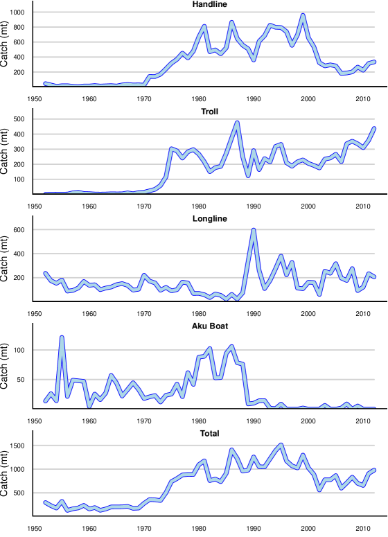
where $m$ is the number of time steps in the catch time series and $\theta=\left\{\widetilde{Y},F_{\widetilde{Y}},Q,\sigma_{P},\sigma_{F},\sigma_{Y}\right\}$ is a vector of model parameters (Table 1). The model is implemented in ADMB-RE (Fournier et al. 2012) and applied to a 61 year ($m=61$) time series of reported commercial catch by four fishing gears from 1952 through 2012 (Figure A.3). Data preparation is described in Appendix A. Noncommercial fishers land substantial quantities of YFT, but reliable data from this sector of the fishery are not currently available. The effects of omitting the noncommercial catch is discussed briefly in Appendix D. All computer code and data files discussed in this paper can be found at Github: https://github.com/johnrsibert/XSSA.git.

Results

Table 2 compares 6 different models using three index of abundance assumptions and two assumed values of the standard deviation of the $r$ prior, $\sigma_{r}$. Models without an index of abundance do not converge to solutions as indicated by the values of $|G|_{max}$. Values of $-\log L$ are lower for models with the loose constraint on $r$ ($\sigma_{r}=0.8$) than for equivalent models with the tight constraint on $r$ ($\sigma_{r}=0.1$). Models with $\sigma_{r}=0.1$ estimate higher values of $F_{\widetilde{Y}}$ and the calculated values of $r$ are, of course, closer to the prior.

Table 2: Results for 6 different models using three abundance indices and two constraints on $r$. The first section of the table shows model diagnostics. $-\log L$ is the negative logarithm of equation 11; lower values indicate better fits to the data. $|G|_{max}$ is the maximum gradient of the likelihood with respect to the parameters; values of $|G|_{max}>10^{-4}$ (1e-04) indicate lack of model convergence. $n$ is the number of parameters estimated. All values are reported to three significant figures.

Index Region	2	4	None	2	4	None
$-\log L$	157.54	128.73	789.98	170.78	130.36	317.17
$n$	6	6	5	6	6	5
$|G|_{max}$	9.72e-06	8.65e-06	0.266	3.5e-05	5.44e-06	0.455
$\widetilde{Y}$	1180	765	3040	1030	928	1490
$F_{\widetilde{Y}}$	0.0235	0.0815	0.248	0.207	0.225	0.239
$Q$	0.438	0.00699	—	0.025	0.00288	—
$\sigma_{P}$	0.112	0.0699	0.00203	0.167	0.0789	0.00366
$\sigma_{F}$	0.323	0.346	0.328	0.321	0.345	0.336
$\sigma_{Y}$	0.393	0.382	0.389	0.394	0.382	0.393
$r$	0.047	0.163	0.495	0.415	0.45	0.478
$K$	100000	18800	24500	9970	8240	12500
$\bar{F}_{5}$	0.0104	0.181	0.388	0.19	0.429	0.334
$p_{0}$	0.197	0.197	0.197	0.197	0.197	0.197
$\tilde{r}$	0.486	0.486	0.486	0.486	0.486	0.486
$\sigma_{r}$	0.8	0.8	0.8	0.1	0.1	0.1

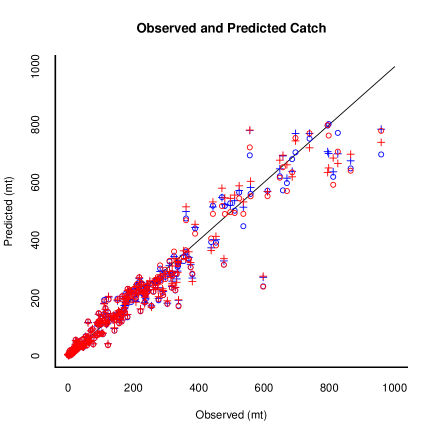
Models with region 2 indexing and region 4 indexing appear to be equally capable of accurately predicting catch, Figure 2. Low catches are predicted accurately, but some high catches are estimated with larger errors, as is expected with log-normal errors. See Figure C.1 for more detail.

Figure 2: Plot of predicted catch on observed catch for two indices of abundance. Open circles (o) indicate region 2 index; plus (+) symbols indicate region 4 index. Blue indicates $\sigma_{r}=0.8$; red indicates $\sigma_{r}=0.1$. The black line has a slope of 1 and passes through the origin.

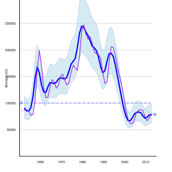
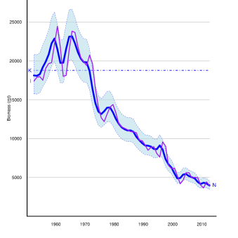
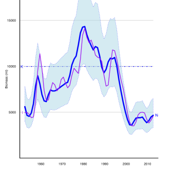
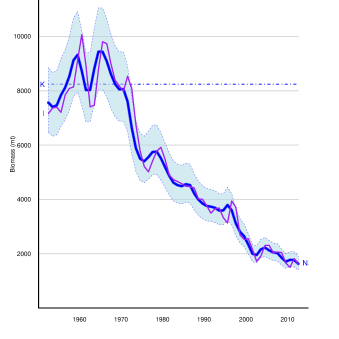
Estimated biomass tracks abundance indices for all models, Figure 3, and the abundance indices lie within the process error of the biomass trend. The maxima of the estimated biomass trends may exceed the estimated equilibrium biomass ($K$) for varying periods of time for all models. In the case of the model with region 2 index $\sigma_{r}=0.8$, the estimated biomass exceeds $K$ for most of the time series.

A. Region 2 index; $\sigma_{r}=0.8$	B. Region 4 index; $\sigma_{r}=0.8$
C. Region 2 index; $\sigma_{r}=0.1$	D. Region 4 index; $\sigma_{r}=0.1$

Figure 3: Predicted biomass trends with different indices of abundance and values of $\sigma_{r}$. Blue lines indicate the estimated biomass in metric tons (mt); purple lines indicates the index of abundance. The light blue shaded areas represent the process error as $\pm 2\sigma_{P}$. The equilibrium biomass $K$ is indicated by the blue dot-dash line. Note that the scale of the ordinate is different in each panel.

The average total YFT catch in the MHI for the most recent 5 years is 818 mt. The estimated $\widetilde{Y}$ is higher than this average for all models except the region 4 index with $\sigma_{r}=0.1$. The estimated average fishing mortality for the last 5 years is below the estimated $F_{\widetilde{Y}}$ for both region 2 models, but above estimated $F_{\widetilde{Y}}$ for the region 4 models; see Table 2.

Discussion

Failure of the model to converge to a solution without an index of abundance (Table  2) indicates that the data lack sufficient information for this model. An informative prior constraint on a parameter and an index of abundance are additional assumptions that provide information to a model to constrain its behavior. Interpretations of these two assumptions are quite different. Assuming a prior value for $r$ implies a priori knowledge of stock productivity, and imposing a low standard deviation around the prior implies a high level of certainty about its value. On the other hand, assuming that local stock size is proportional to stock size in a larger geographic range implies that factors mediating the abundance of the local stock are similar to those mediating the abundance in the larger area.

MFCL Regions 2 and 4 differ from one another in their oceanography, ecology and fisheries (Appendix B). Region 2 is outside the center of abundance for YFT in the WCPO, appears to have a relatively small YFT stock, and Davies et al. (2014) estimate that region 2 has experienced relatively minor fishery impact. In contrast, region 4 straddles the equatorial center of YFT abundance, appears to have a larger stock, hosts some of the largest fisheries in the WCPO, produces a large proportion of the total WCPO yellowfin catch, and Davies et al. (2014) estimate that region 4 has experienced the largest impact of the fishery of any of the MFCL regions. Region 2, therefore, is the best a priori choice for an index of abundance.

The random walk representation of fishing mortality enables the model to compute accurate values of $F_{g,t}$. The zero-inflated log normal observation error and the separation of fishing fleets enable the model to interpret low (or zero) catches as changes in $F_{g,t}$ rather than as episodes of low stock size. These features enable the model to estimate catch from the estimated stock extremely accurately.

Current catches ($\bar{Y}_{5}=818$) are less than model estimates of maximum sustainable yield ($\widetilde{Y}$) for all model variants. Estimates of current fishing mortality ($\bar{F}_{5}$) are less than estimates of fishing mortality at maximum sustainable yield ($F_{\widetilde{Y}}$) for all models with region 2 index of abundance. If fishery managers were to adopt $\widetilde{Y}$ and $F_{\widetilde{Y}}$ as management reference points, the conclusion would be that the local stock is not overfished and that overfishing is not occurring.

The model presented here is a promising, if preliminary, approach to assessing a local portion of a larger fish stock in a way that provides useful advice to local fisheries managers. The current model is clearly in need of further development. Estimates of noncommercial catch (and possibly their observation error) should be included in the data. The issue of selecting an appropriate index of abundance should be resolved. One hopes that the next round of WCPFC stock assessments will realign the MFCL regions to be more consistent with the Longhurst (1998) ecological provinces so that the entire Hawaiian Archipelago lies within a single stock assessmemt region. A region that aligns approximately with the North Pacific Tropical Gyre Province would be the best choice for an index of abundance for the MHI.

Acknowledgements. This work was initiated under a contract from the Western Pacific Regional Fisheries Managment Council. I thank the Council for its generous support and Council Staff Paul Dalzell and Eric Kingma for encouraging me to take on this challenging project. Special thanks are due to David Itano for sharing insights into the biology of yellowfin tuna and into small-boat fisheries in Hawaii, to Reginald Kokubun of the State of Hawaii, Division of Aquatic Resources, Department of Land and Natural Resources, for supplying catch report data from the Commercial Marine Landings data base, to Keith Bigelow and Karen Sender of NOAA Pacific Island Fisheries Science Center for supplying logbook reporting data and from the PIFSC data base. Thanks also to John Hampton of the Secretariat of the Pacific Community, Oceanic Fisheries Programme, for making available MULTIFAN-CL output files from the latest Western and Central Pacific Fisheries Commission yellowfin tuna stock assessment, and to Nick Davies for advice on interpreting those files.

References

Carruthers, T. and M. McAllister. 2011. Computing prior probability distributions for the intrinsic rate of increase for Atlantic tuna and billfish using demographic methods. Collect. Vol. Sci. Pap. ICCAT, 66(5): 2202-2205.

Davies, N., S. Harley, J. Hampton, S. McKechnie. 2014. Stock assessment of yellowfin tuna in the western and central pacific ocean. WCPFC-SC10-2014/SA-WP-04.

Fournier, D. A., H.J. Skaug, J. Ancheta, J.Sibert, J. Ianelli, A. Magnusson, M. N. Maunder, A. Nielsen. 2012. AD Model Builder: using automatic differentiation for for statistical inference of highly parameterized complex nonlinear models. Optimization Methods and Software 27, 233–249.

DLNR. 2011. HMRFS Newsletter. Hawaii Department of Land and Natural Resources.https://dlnr.hawaii.gov/dar/fishing/hmrfs/

Longhurst, A. 1998. Ecological Geography of the Sea. Academic Press, San Diego. 398pp.

Nielsen, A., C. Berg. 2014. Estimation of time-varying selectivity in stock assessments using state-space models. Fisheries Research 158:96-101.

Quinn, T, R. Deriso. 1999. Quantitative fish dynamics. Oxford University Press, New York.

Rooker, J.R., R. J. D. Wells, D. G. Itano, S. R. Thorrold, J. M. Lee. 2016. Natal origin and population connectivity of bigeye and yellowfin tuna in the Pacific Ocean. Fish. Oceanogr. 25, 277-291.

Schaefer, M. B. 1954. Some aspects of the dynamics of populations important to the management of the commercial marine fisheries. IATTC Bull. 1:27-56.

Senina, I., P. Lehodey, B. Calmettes, S. Nicol, S. Caillot, J. Hampton and P. Williams. 2015. SEAPODYM application for yellow tuna in the Pacific Ocean. WCPFC-SC11-2015/EB-IP-01.

Skaug, H., Fournier, D., 2006. Automatic approximation of the marginal likelihood in non-Gaussian hierarchical models. Computational Statistics & Data Analysis 51, 699–709.

Wilson, P. T. 2011. AKU!. Xlibris, USA. 368pp. ISBN 978-1-4568-5904-6.

Appendix A Data preparation

Figure A.1: Yellowfin catch in metric tonnes by principle fisheries operating in the Main Hawaiian Islands from the State of Hawaii Commercial Marine Landings Data. The red tick marks on the abscissa indicate quarters where reported catches were zero.

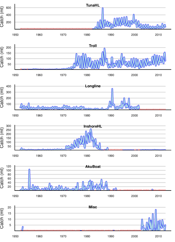
The State of Hawaii Department of Land and Natural Resources Commercial Marine Landings data base (CML) from 1949 through 2014 is the primary source of data used in this analysis. This database documents the continuous 65 year history of commercial fishing in Hawaii.

The CML catch reports were aggregated into the following gear categories: “Aku boat”, “Bottom/inshore HL”, “Longline”, “Troll”, “Tuna HL”, “Casting”, “Hybrid”, “Shortline”, “Other”, and “Vertical line”. For this analysis catches by “Casting”, “Hybrid”, “Shortline”, “Other”, and “Vertical line” are combined into a new category, “Misc”. Landing in the “Misc” category are highest after year 2000 and less than 2% of the total landings. The catch time series for the CML data are shown in Figure A.1. The “Bottom/inshore HL” and “Tuna HL” are both handline gears and the data for these two gear types were combined at the suggestion of the CML database administrator. The “Aku Boat” gear type refers to storied Japanese-style pole and line fishery that operated in Hawaii through th 1980s (Wilson 2011). The Aku Boats target skipjack tuna (Katsuwonus pelamis), but yellowfin were occasionally landed as incidental catch. Some time series contain sustained periods of zero catch which reflect the development and subsequent shift away from a specific gear type. It is assumed that these declines in catches represent “collapse” of a fishery due to social and economic factors rather than to a decline of YFT stocks. Similarly, some time series are punctuated by brief episodes (one or two quarters in length) of zero catches. Again, it is assumed that these zero catches are not caused by low stock size.

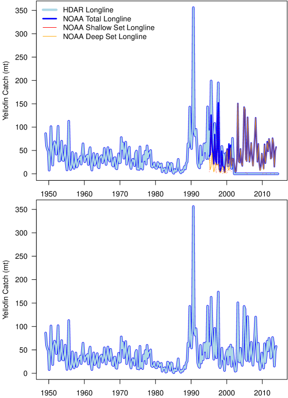
The Hawaii-based longline fishery began a rapid expansion in the late 1980s, and the United States National Oceanic and Atmospheric Administration (NOAA) began to collect data from the longline fleet under a federally mandated logbook program in 1990. The CML longline data were augmented by NOAA longline log sheet data from 1995 through 2013. NOAA distinguishes deep sets, targeting bigeye tuna (Thunnus obesus), and shallow sets, targeting swordfish (Xiphias gladius) in the data. The CML data do not distinguish between deep and shallow sets. Since the longline fleet ranges widely in the North Pacific Ocean, only catches reported in the United States EEZ around Hawaii east of 162^∘W longitude were included in the data. Figure A.2 shows the correspondence between the CML and NOAA time series. The combined deep plus shallow catches from NOAA align fairly well with the overlapping CML data. The simple average of the CML data with the combined NOAA deep plus shallow data appears to be roughly the same trajectory as the constituent time series. Yellowfin is currently considered an incidental catch in the longline fishery.

Figure A.2: Comparison between CML and NOAA longline time series. The upper panel shows the NOAA deep and shallow set data superimposed on the HDAR data. The lower panel shows the time series produced by a simple average of the CML data and the sum of the NOAA deep and shallow catches.

Catch data from the CML and NOAA longline data bases were initially aggregated by quarter of the calendar year. All catch time series exhibit annual cycles suggesting strong seasonal signals in the catches by all gears. To avoid the need to estimate autocorrelation matrices for each time series and to minimize the number of zero catch observations, the quarterly time series were aggregated into the annual time series shown in Figure A.3 and used in this analysis.

Figure A.3: Four gear type catch time series used in the assessment model.

Appendix B Abundance indices and offline coupling

Using the output of one model to constrain a second model is sometimes referred to as “offline” coupling. The output from two quite different models of WCPO yellowfin, SEAPODYM and MULTIFAN-CL, could potentially be used as indices of abundance. Both models are age structured, spatially structured, and have been applied to YFT. SEAPODYM is an ocean basin scale model with 1^∘ spatial resolution, whereas the MULTIFAN-CL yellowfin assessment model is constrained to the western Pacific and partitions the model domain into 9 regions, Figure B.1. The spatial resolution of the SEAPODYM model would make it an ideal candidate for computing an index of abundance, but the model and its application to yellowfin are still under active development (Senina et al, 2015). The 2014 MULTIFAN-CL assessment (Davies et al. 2014) has been officially adopted by the WCPFC as the assessment on which regional conservation and management measures are based.

Figure B.1: Regional structure used in the 2014 WCPFC YFT stocks assessment from Davies et al. (2014).

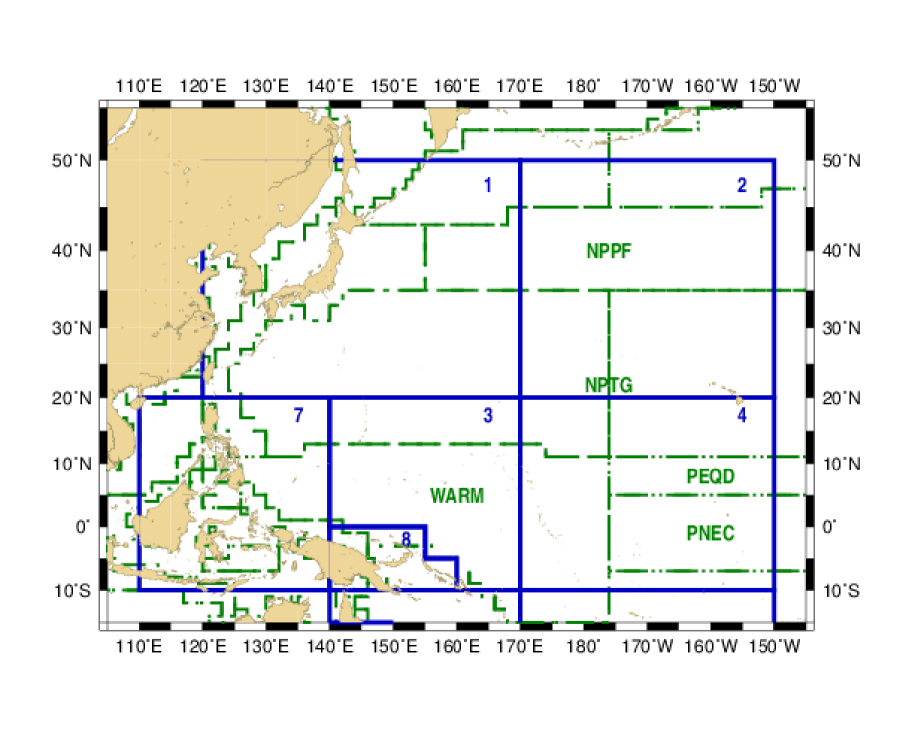
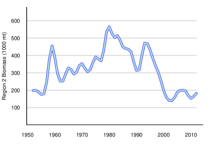
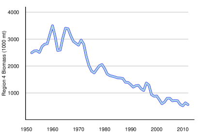
The Hawaiian archipelago lies in the eastern extension of Longhurst’s (1998) North Pacific Tropical Gyre Province (NPTG), Figure B.2. The boundary between MFCL regions 2 and 4 splits both MHI and the NPTG. Region 2 includes the northern extent of the range of YFT. The MFCL assessment concludes that the YFT biomass is relatively low and that the impact of the WCPO fisheries has been relatively minor. In contrast, region 4 lies in primarily in the Western Pacific Warm Pool Province, includes the core of the YFT range in the Pacific, and supports some of the most intense tuna fisheries in the world. MFCL estimates that the impact of the fisheries on the YFT stock in region 4 to be one among the highest of all MFCL regions, and it is likely that overfishing is occuring. The estimated biomass trends in these two regions are quite different, Figure B.3. Selecting a specific biomass time series for an index of abundance for the MHI stock implicitly assumes that the ecology and productivity of the index population is comparable to the MHI. On the basis of low levels of exploitation and the location of the Hawaiian archipelago in the NPTG, MFCL region 2 would seem a priori to be the best choice of a for computing an index of abundance.

Figure B.2: Map of the central north Pacific Ocean showing selected MULTIFAN-CL stock assessment regions (blue lines and numbers) and Longhurst (1998) ecological provinces (dashed green lines and labels); NPFF, North Pacific Transition Zone Province; NPTG, North Pacific Tropical Gyre Province; WARM, Western Pacific Warm Pool Province; PEQD, Pacific Equatorial Divergence Province; PNEC, North Pacific Equatorial Countercurrent Province.

MFCL Region 2	MFCL Region 4

Figure B.3: Estimated biomass trends in MULTIFAN-CL regions 2 and 4 (Davies, et al. 2014).

Appendix C Additional Diagnostics

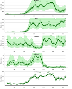
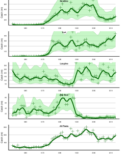
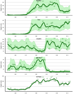
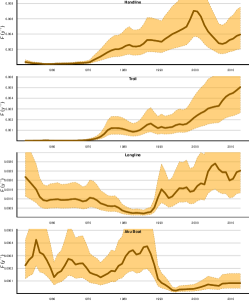
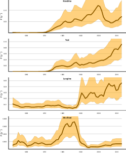
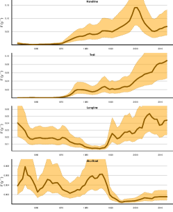
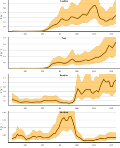
Figures C.1 and C.2 show the trends in estimated catch add fishing mortality with different indices of abundance and values of the $r$ prior, $\sigma_{r}$. The ordinate in each panel is scaled to the specific gear type.

$\sigma_{r}=0.8$
Region 2 Index	Region 4 Index
$\sigma_{r}=0.1$
Region 2 Index	Region 4 Index

Figure C.1: Trends in observed (+) and estimated catch (solid green line). The light green shaded areas represent the process error as $\pm 2\sigma_{Y}$.

$\sigma_{r}=0.8$
Region 2 Index	Region 4 Index
$\sigma_{r}=0.1$
Region 2 Index	Region 4 Index

Figure C.2: Trends in estimated fishing mortality (solid brown line). The orange shaded areas represent the process error as $\pm 2\sigma_{F}$.

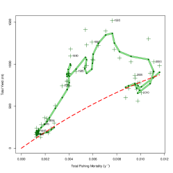
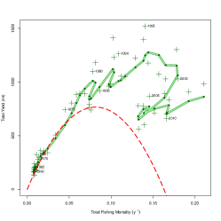
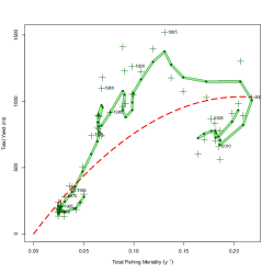
Figure C.3 places the model results in a fishery management context. The parabolic dashed red lines indicate the theoretical yield from a population with logistic growth. The maximum yield if the population were at equilibrium would occur at the peak of the parabola. There are many possible equilibria, but the maximum equilibrium yield has been labeled “Maximum Sustainable Yield”, $\widetilde{Y}$, in the fisheries literature. The parameter $F_{\widetilde{Y}}$ is the fishing mortality that would produce $\widetilde{Y}$ at equilibrium.

Region 2; $\sigma_{r}=0.8$	Region 4; $\sigma_{r}=0.8$
Region 4; $\sigma_{r}=0.1$	Region 4; $\sigma_{r}=0.1$

Figure C.3: Estimated production curves showing catch plotted against estimated fishing mortality with different indices of abundance and values of $\sigma_{r}$. The green line and dark green dots are estimated catch. The green $+$ symbols are the observed catch annotated with the year. The dashed red line is the theoretical equilibrium yield. Note that the scale of the abscissa is different in each panel, and the ordinate has been scaled to the observed catch.

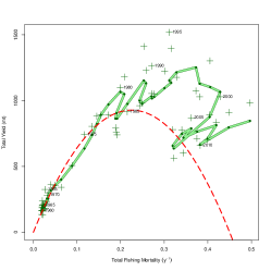Figure C.4 shows the frequency distributions of the parameter estimates obtained by sampling the output of $10^{6}$ Markov Chain Monte Carlo simulations. Some parameters are clearly estimated more accurately than others. The process and observation error estimates have well defined modes and appear to be normally distributed around their point estimates. The distributions of other parameters depends on the abundance index and value of $\sigma_{r}$. Figure C.4 also demonstrates the pervasive (some might say pernicious) effects of using an informative prior on $r$.

A. Region 2; $\sigma_{r}=0.8$

 
B. Region 4; $\sigma_{r}=0.8$

 
C. Region 2; $\sigma_{r}=0.1$

 
D. Region 4; $\sigma_{r}=0.1$

 

Figure C.4: Posterior distributions of parameter estimates from $10^{6}$ MCMC samples. Black circles and connecting lines are frequencies of the estimates. Blue curves are the theoretical normal distribution of the maximum likelihood estimates computed from the standard deviations estimated from the inverse Hessian matrix at the minimum. Vertical blue dotted lines indicate $\pm 2\sigma$. The solid red curves indicate the effect of the prior on $r$; the vertical red line is the prior.

Table 3: Correlation coefficients between parameter estimates for four models.

A. Region 2; $\sigma_{r}=0.8$ $\widetilde{Y}$ $F_{\widetilde{Y}}$ $\sigma_{P}$ $\sigma_{F}$ $\sigma_{Y}$ $Q$ $r$ $K$ $\widetilde{Y}$ 1.00 $F_{\widetilde{Y}}$ 0.23 1.00 $\sigma_{P}$ 0.13 0.39 1.00 $\sigma_{F}$ 0.01 -0.00 -0.00 1.00 $\sigma_{Y}$ -0.00 0.00 0.00 -0.31 1.00 $Q$ 0.98 0.04 0.06 0.01 -0.00 1.00 $r$ 0.23 1.00 0.39 -0.00 0.00 0.04 1.00 $K$ 0.99 0.07 0.07 0.01 -0.00 1.00 0.07 1.00	B. Region 4; $\sigma_{r}=0.8$ $\widetilde{Y}$ $F_{\widetilde{Y}}$ $\sigma_{P}$ $\sigma_{F}$ $\sigma_{Y}$ $Q$ $r$ $K$ $\widetilde{Y}$ 1.00 $F_{\widetilde{Y}}$ 0.76 1.00 $\sigma_{P}$ 0.23 0.28 1.00 $\sigma_{F}$ 0.04 0.01 -0.02 1.00 $\sigma_{Y}$ -0.02 -0.01 -0.00 -0.26 1.00 $Q$ -0.53 -0.95 -0.25 0.01 0.01 1.00 $r$ 0.76 1.00 0.28 0.01 -0.01 -0.95 1.00 $K$ -0.50 -0.94 -0.26 0.01 0.01 0.99 -0.94 1.00
C. Region 2; $\sigma_{r}=0.1$ $\widetilde{Y}$ $F_{\widetilde{Y}}$ $\sigma_{P}$ $\sigma_{F}$ $\sigma_{Y}$ $Q$ $r$ $K$ $\widetilde{Y}$ 1.00 $F_{\widetilde{Y}}$ -0.01 1.00 $\sigma_{P}$ 0.08 0.33 1.00 $\sigma_{F}$ 0.05 -0.01 -0.02 1.00 $\sigma_{Y}$ -0.02 0.01 -0.01 -0.30 1.00 $Q$ 0.90 -0.38 -0.03 0.05 -0.02 1.00 $r$ -0.01 1.00 0.33 -0.01 0.01 -0.38 1.00 $K$ 0.93 -0.39 -0.05 0.05 -0.02 0.98 -0.39 1.00	D. Region 4; $\sigma_{r}=0.1$ $\widetilde{Y}$ $F_{\widetilde{Y}}$ $\sigma_{P}$ $\sigma_{F}$ $\sigma_{Y}$ $Q$ $r$ $K$ $\widetilde{Y}$ 1.00 $F_{\widetilde{Y}}$ 0.13 1.00 $\sigma_{P}$ 0.07 0.17 1.00 $\sigma_{F}$ 0.08 -0.01 -0.04 1.00 $\sigma_{Y}$ -0.04 0.00 -0.01 -0.26 1.00 $Q$ 0.49 -0.76 -0.08 0.06 -0.03 1.00 $r$ 0.13 1.00 0.17 -0.01 0.00 -0.76 1.00 $K$ 0.53 -0.78 -0.10 0.06 -0.03 0.96 -0.78 1.00

Appendix D Noncommercial Catch

The Main Hawaiian Islands support a large number of noncommercial fishers. There is no catch reporting system and no mandatory marine fishing license. Accurately estimating the noncommercial catch is therefore difficult. The State of Hawaii Department of Land and Natural Resources and the United States National Oceanic and Atmospheric Administration are collaborating to improve survey methods for the Hawai‘i Marine Recreational Fishing Survey (HMRFS). The HMRFS Newsletter (DLNR, 2011) reports that non-commercial catches of YFT range between 2300 and 6900 mt from 2003 through 2010, roughly 3 to 10 times greater than the most recent commercial catch. The assessment model developed here has the capability to augment the reported catch with catch by an additional fleet in proportion to the total reported catch and use the augmented catch in the assessment as if it were reported. Region 2 indexing was used with both loose and tight priors on $r$. Four different multipliers were tested so that the augmented catch was 1, 2, 5, and 10 times total catch.

Tables 4 and 5 summarize the results of fitting the augmented catch. All 8 augmented catch models converge to solutions. The negative log likelihood values are higher than comparable non-augmented fits. A priori one would expect that a fish population capable of producing a higher than reported yield over a 60 year history would have a higher productivity and a higher biomass. These results are generally consistent with this conclusion. The model compensates for the higher catch by estimating higher $\widetilde{Y}$ and higher $K$ in all models, whereas estimates $F_{\widetilde{Y}}$ and $r$ are relatively unchanged by the augmented catch. Estimates of $\bar{F}_{5}$ increase in models with $\sigma_{r}=0.8$ but change very little in models with $\sigma_{r}=0.1$. The $\sigma_{r}=0.8$ model estimates that the fishery is sustainable with a total yield about 5 times the current reported yield. The $\sigma_{r}=0.1$ model forces a much higher $F_{\widetilde{Y}}$. In consequence, this form of the model estimates a sustainable fishery with yields at least 10 times current reported yield.

This simple catch augmentation simulation indicates that unreported noncommercial catch causes this model to underestimate maximum sustainable yield and the fishing mortality at maximum sustainable yield when applied to the available reported catch data. To put this conclusion in a different context, fishers should report their catch if they want a higher yield from a managed fishery.

Table 4: Results of fitting the model to 4 different multiples of the total catch using MFCL Region 2 as an index of abundance and a loose prior on $r,\sigma_{r}=0.8$, comparable to Table 2. See Table 1 for definitions of all variables.

Multiplier	1	2	5	10
	k1	k2	k5	k10
$-\log L$	181.75	181.77	181.97	182.84
$n$	6	6	6	6
$|G|_{max}$	8.32e-05	6.87e-05	6.24e-05	5.6e-05
$\widetilde{Y}$	2240	2740	2810	3070
$F_{\widetilde{Y}}$	0.0237	0.0237	0.0237	0.0248
$Q$	0.819	1	1	1
$\sigma_{P}$	0.112	0.112	0.112	0.113
$\sigma_{F}$	0.295	0.295	0.295	0.294
$\sigma_{Y}$	0.358	0.358	0.358	0.358
$r$	0.0474	0.0474	0.0475	0.0495
$K$	189000	232000	237000	248000
$\bar{F}_{5}$	0.0111	0.0136	0.0270	0.0485
$p_{0}$	0.197	0.197	0.197	0.197
$\tilde{r}$	0.486	0.486	0.486	0.486
$\sigma_{r}$	0.8	0.8	0.8	0.8
$\bar{Y}_{5}$	1630	2450	4890	8960

Table 5: Results of fitting the model to 4 different multiples of the total catch using MFCL Region 2 as an index of abundance and a tighter prior on $r,\sigma_{r}=0.1$, comparable to Table 2. See Table 1 for definitions of all variables.

Multiplier	1	2	5	10
	k1	k2	k5	k10
$-\log L$	194.64	194.63	194.58	194.56
$n$	6	6	6	6
$|G|_{max}$	9.36e-05	4.46e-05	2.7e-05	7.46e-05
$\widetilde{Y}$	2060	3110	6260	11500
$F_{\widetilde{Y}}$	0.208	0.208	0.208	0.208
$Q$	0.0495	0.0747	0.15	0.277
$\sigma_{P}$	0.169	0.169	0.167	0.167
$\sigma_{F}$	0.291	0.291	0.291	0.291
$\sigma_{Y}$	0.357	0.357	0.357	0.358
$r$	0.415	0.415	0.416	0.416
$K$	19800	29900	60200	111000
$\bar{F}_{5}$	0.191	0.191	0.191	0.191
$p_{0}$	0.197	0.197	0.197	0.197
$\tilde{r}$	0.486	0.486	0.486	0.486
$\sigma_{r}$	0.1	0.1	0.1	0.1
$\bar{Y}_{5}$	1630	2450	4890	8960
$\bar{C}$	1380	2070	4130	7560