Fluctuations in ultra-relativistic heavy ion collisions

Fluctuations are one of the main probes of the physics of the new state of hot and dense nuclear matter called the Quark Gluon Plasma (QGP) which is created in the ultra-relativistic heavy ion collisions. In this dissertation we extend and improve upon the existing descriptions of heavy ion collisions in three different directions: we study the new signatures of initial state fluctuations, the propagation of perturbations in the early stages of the collision, and the effect of thermal fluctuations on the hydrodynamic expansion of the QGP.

First, in Chapter 3 we study initial state fluctuations by examining the complete statistical information contained in the two-particle correlation measurements in hydrodynamic simulations of Pb+Pb collisions at the CERN Large Hadron Collider (${\sqrt{s_{\scriptscriptstyle NN}}}=2.76\,{\rm TeV}$). We use Principal Component Analysis (PCA) to decompose the spectrum of harmonic flow, $v_{n}(p_{T})$ for $n=0\text{--}5$, into dominant components. The leading component is identified with the standard event plane $v_{n}(p_{T})$, while the subleading component describes additional fluctuations in the two-particle correlation function. We find good geometric predictors for the orientation and the magnitude of the leading and the subleading flows. The subleading $v_{0}$, $v_{1}$, and $v_{3}$ flow harmonics are shown to be a response to the radial excitation of the corresponding eccentricity $\varepsilon_{n}$. In contrast, for $v_{2}$ the subleading flow in peripheral collisions is dominated by the nonlinear mixing between the leading elliptic flow and radial flow fluctuations. Nonlinear mixing also plays a significant role in generating subleading $v_{4}$ and $v_{5}$ harmonics. The PCA gives a systematic way of studying the full information of the two-particle correlation matrix and identifying the subleading flows, which we show are responsible for factorization breaking in hydrodynamics.

Second, in Chapter 4 we study the thermalization and hydrodynamization of fluctuations at the early stages of heavy ion collisions. We use leading order effective kinetic theory, accurate at weak coupling, to simulate the pre-equilibrium evolution of transverse energy and flow perturbations. For the short evolution we can use a linear response theory to construct the pre-equilibrium Green functions. Then the energy-momentum tensor at a time when hydrodynamics becomes applicable can be expressed as a linear convolution of response functions with the initial perturbations. We propose combining effective kinetic theory with weak coupling initial state models, such as IP-Glasma, to model the complete pre-thermal evolution from saturated nuclei to hydrodynamics in a weak coupling framework.

Last, in Chapter 5 we consider out-of-equilibrium hydrodynamic fluctuations in the expanding QGP. We develop a set of kinetic equations for a correlator of thermal fluctuations which are equivalent to nonlinear hydrodynamics with noise. We first show that the kinetic response precisely reproduces the one-loop renormalization of the shear viscosity for a static fluid. We then use the hydro-kinetic equations to analyze thermal fluctuations for a Bjorken expansion. The steady state solution to the kinetic equations determine the coefficient of the first fractional power of the gradient expansion ($\propto 1/(\tau T)^{3/2}$), which was computed here for the first time. The formalism of hydro-kinetic equations can be applied to more general background flows and coupled to existing viscous hydrodynamic codes to incorporate the physics of hydrodynamic fluctuations.

Contributions of Authors

Chapter 3 contains published material of the co-authored papers [1] and [2]. I, the present author, contributed significantly to all parts of this work and, in particular, was responsible for performing the PCA and finding the optimal geometric predictors (including writing the necessary computer code). I also offered the interpretation of the subleading elliptic flow as a response to radial size modulations of the background $\varepsilon_{2}$ in Sec. 3.7.2. The hydrodynamic simulations of heavy ion collisions used in this publication were done by others.

Chapter 4 is a partial reproduction of the published article written with co-authors [3]. I made significant contributions in the preparation of this paper. I identified the causality constrains and constructed the coordinate space Green functions. I also found the analytic limit of the response to small wavenumber perturbations in Sec. 4.4.1. I contributed to, but was not the main author of the kinetic theory simulation code used for this paper.

Chapter 5 is a reproduction of the published article with collaborators [4]. I contributed to all stages of this work. I reproduced the renormalization results for the static fluid in Sec. 5.2 and I obtained the final numerical results of finite noise contributions for the Bjorken background, which are summarized in Table 5.1.

The introductory and final chapters of this dissertation (Chapters 1, 2 and 6) were not published before, except for the figures taken from the referenced sources.

Publications

• A. Mazeliauskas and D. Teaney, Subleading harmonic flows in hydrodynamic simulations of heavy ion collisions, Phys. Rev. C91, 044902 (2015) [1]. Copyright (2015) by the American Physical Society

• A. Mazeliauskas and D. Teaney, Fluctuations of harmonic and radial flow in heavy ion collisions with principal components, Phys. Rev. C93, 024913 (2016) [2], Copyright (2016) by the American Physical Society

• L. Keegan, A. Kurkela, A. Mazeliauskas and D. Teaney, Initial conditions for hydrodynamics from weakly coupled pre-equilibrium evolution J. High Energ. Phys. 08, 171 (2016) [3]. Copyright (2016) by authors.

• Y. Akamatsu, A. Mazeliauskas and D. Teaney, A kinetic regime of hydrodynamic fluctuations and long time tails for a Bjorken expansion, Phys. Rev. C95, 014909 (2017) [4]. Copyright (2017) by the American Physical Society

Chapter 1 Foreword

For the most of science history physicists investigated phenomena governed by just two fundamental forces—gravity and electromagnetism. Gravity holds together the large scale structures like planets and galaxies, while electromagnetic interactions bond atoms together. Electromagnetic forces are also responsible for many different phases of matter and endless diversity of chemical compounds.

The turn of the twentieth century marked a new era in physics with the discovery of subatomic particles, e.g. electron and proton. Two new and short ranged forces, i.e. acting only at subatomic distances, were introduced: a weak interaction to explain the $\beta$ decay [6] and a strong interaction to provide a necessary bond between protons and neutrons in the nucleus [7]. In the following decades huge theoretical and experimental advances lead to a detailed description of electromagnetic, weak and strong interactions in terms of quantum field theories [8, 9, 10, 11, 12, 13]. This description together with the list of discovered particles forms a highly successful particle physics framework known as the Standard Model [14, 15, 16, 17]. It is still an ongoing research effort to incorporate gravity on the same footing as other interactions [18].

The quantum field theory which describes the strong interactions between the fundamental constituents of a nucleus (quarks and gluons) is called the Quantum Chromodynamics (QCD) [14, 15, 17]. Unlike the Quantum Electrodynamics, QCD is a non-abelian gauge theory and the particular number of quark flavors and color charges make QCD look weak at very short distances—a phenomena known as asymptotic freedom [19, 20, 21]. Therefore certain processes at high energy, which probe the small distance limit of the QCD, can be accurately described by perturbative expansion in the coupling constant $\alpha_{s}$. In contrast, at large distances (or small energies) the strength of the strong interaction grows and new, non-perturbative phenomena appear, e.g. color confinement—quarks and gluons are hidden in color neutral hadrons [22, 23, 24].

Although the fundamental QCD equations of motion are known, most of their physical consequences remain an unsolved mathematical problem [25]. Thanks to the complex nature of the strong force and many body interactions, a hot and dense QCD medium is a fascinating phase of matter with unprecedented properties [26, 27]. One very successful approach of studying the strongly interacting QCD has been the discretized QCD formulation on a lattice [22]. With the progress of numerical methods and computational power, Lattice QCD is able to reproduce and even predict some properties of the QCD, notably, the hadron spectrum and the QCD equation of state [28, 29]. However, transport properties of the QCD medium or simulations at the non-zero baryon chemical potential are very difficult in Lattice QCD [29]. String theory research (which too has its roots in the attempt to describe the non-perturbative phenomena of strong interactions [30]) produced a new perspective of strongly coupled systems known as a gauge/gravity duality [31]. This holographic duality allows to map the non-perturbative regime of certain gauge theories to classical supergravity in higher dimensions, where calculations are tractable [32]. Although no dual of the QCD is known, other gauge theories are used to infer generic features of strongly coupled systems, e.g. viscosity over entropy ratio $\eta/s$  [33, 34].

Physics is an empirical science and its ultimate guidance principle must be the experiment. To create matter where the asymptotic degrees of freedom are quarks and gluons one has to reach energies and densities exceeding that of nucleus core [35]. Such state of matter known as the Quark Gluon Plasma (QGP) is believed to have existed during the first few microseconds of the Big bang and possibly exists at the center of neutron stars [36, 37, 38, 39]. On Earth the only way of creating such extreme conditions is in the relativistic hadron colliders [40]. Nuclei of heavy elements, e.g. lead (Pb) or gold (Au), are accelerated to ultra-relativistic energies and collided, momentarily creating a droplet of melted nuclear matter which evaporates into a cloud of hadrons in less than $\sim 10^{-22}$ seconds. The debris of the collision are then used to infer the interesting properties of the ultra-dense nuclear matter. Such events or “little Big bangs” are repeated billions of times, thus making statistical analysis of the QGP evolution possible.

In the last couple decades the successful hadron collision programs in the US and Europe produced a wealth of experimental data, many surprising results, and new understanding of the behavior of matter under the extreme conditions. Heavy ion collisions are a dynamical and multistage process, which requires a sophisticated description of every stage of the collision: the initial impact, creation and equilibration of the QGP, the fast QGP expansion and cooling down, and the transition from quarks and gluons into the observed hadrons. To make the problem more tractable, the different regimes of the QCD medium are treated in a number of theoretical limits, which have become sizable subfields in their own right (Color Glass Condensate, relativistic hydrodynamics, gauge/gravity duality of QCD-like theories, finite temperature QCD, etc. [41]). The contrasting pictures of different stages of the heavy ion collision evolution is not unlike a famed group of blind men touching an elephant—individual descriptions might look contradictory, but when combined correctly, a remarkably successful model of the expanding QGP fireball emerges.

In this dissertation I will review my contributions to the physics of heavy ion collisions, which, needless to say, depend on the many decades of experimental and theoretical work done before. Specifically, together with collaborators I worked on the fate of initial and thermal fluctuations in the expanding QGP medium. In Chapter 2, I give a short introduction to the main components of heavy ion physics and the outline of the three research directions addressed in this manuscript. In Chapter 3, I present a published work on the Principal Component Analysis of harmonic flow and factorization breaking [1, 2]. Chapter 4 covers a published work on the QGP equilibration in a weak coupling framework [3]. Finally in Chapter 5, I present my work with collaborators on the effects of thermal fluctuations on the hydrodynamic expansion of the QGP [4]. In Chapter 6, I conclude with a short summary of the conducted work and an outlook.

Chapter 2 Introduction

2.1 Overview

Ultra-relativistic heavy ion collisions is nearly half a century old subject [42]. Below we touch only on the recent development of the field driven by discoveries at RHIC and LHC over the past fifteen years. There is a considerable body of terminology specific to this field, but to avoid interrupting the discussion definitions of the main concepts in heavy ion collisions are given separately in Sec. 2.2.

The Relativistic Heavy Ion Collider (RHIC) at Brookhaven National Laboratory in the United States was built with the purpose of mass production of the new state of matter named the Quark Gluon Plasma (QGP) [42]. Since the start of operation in 2000, RHIC has been exploring a number of different ion systems, Au-Au, Cu+Cu, U+U, and etc., at various collisions energies ${\sqrt{s_{\scriptscriptstyle NN}}}=8\text{-}200\,\text{GeV}$ [43]. This makes the RHIC a versatile machine and particularly well suited for mapping out the phase diagram of the dense QCD matter. The ongoing Beam Energy Scan program (BES) is searching for the QCD critical point—a conjectured end point of the first order phase transition line between the QGP and the hadronic matter [44]. In 2010, the Large Hadron Collider (LHC) at CERN in Switzerland has also started a heavy ion collision program [40, 45]. With higher achievable collision energies (${\sqrt{s_{\scriptscriptstyle NN}}}=2.76\text{-}5.02\,\text{TeV}$ for Pb+Pb), the LHC can create a hotter, larger and longer lasting QGP droplets. The larger space-time volume of QGP medium allows physicists to understand better the bulk properties of hot nuclear matter. In fact, thanks to the high collision energies, measurements of high multiplicity p+Pb and p+p collisions suggest the formation of a QGP fireball even in smaller systems, defying all expectations [46, 47, 48].

Figure 2.1: Illustration of the overlap region (shaded area) of two colliding nuclei (circles). The arrows indicate the hydrodynamic flow. (a) The event averaged “almond shaped” overlap of peripheral collisions driving the elliptic flow $v_{2}$. (b) Triangular deformations due to event-by-event fluctuations causing the triangular flow $v_{3}$.

Figure 2.2: The early years of soft heavy ion observables in the RHIC. Figure taken from Ref. [49]

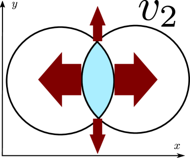
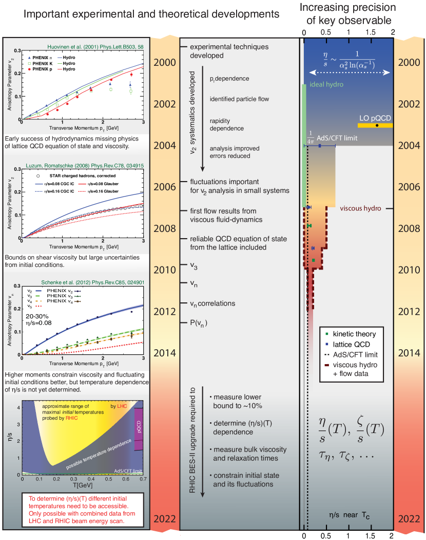
Since the start of the RHIC over 15 years ago, heavy ion physics has progressed tremendously (see the timeline of RHIC physics in Fig. 2.2). The first results of Au+Au collisions at RHIC showed that the produced particle distribution in the plane transverse to the beam has a significant azimuthal anisotropy quantified by the elliptic flow coefficient $v_{2}$

$$v_{2}=\frac{\left<p_{x}^{2}\right>-\left<p_{y}^{2}\right>}{\left<p_{x}^{2}\right>+\left<p_{y}^{2}\right>},$$ (2.1)

where $\left<p_{x}^{2}\right>$ and $\left<p_{y}^{2}\right>$ are momentum averages of observed particles relative to the event plane (see Fig. 2.1(a)) [50]. The presence of the elliptic flow was a strong evidence that QGP expansion is driven by hydrodynamic pressure gradients. In peripheral collisions the average overlap of two colliding nuclei is “almond shaped” and the pressure gradients are the largest along the short axis of the ellipsoid. Then anisotropically flowing medium emits particles boosted in the flow direction and therefore the observed particles have a momentum anisotropy approximately proportional to the initial elliptic deformation, or eccentricity, $\varepsilon_{2}$

$$\varepsilon_{2}=-\frac{\left<x^{2}\right>-\left<y^{2}\right>}{\left<x^{2}\right>+\left<y^{2}\right>},\quad v_{2}\propto\varepsilon_{2}.$$ (2.2)

Here $\left<x^{2}\right>$ and $\left<y^{2}\right>$ are coordinate averages in the center of mass frame of the overlap energy density. At the early years of RHIC, observed momentum anisotropy was reasonably well described by modeling QGP as ideal fluid (see Fig. 2.2 top left). Later, the importance of viscous effects was recognized and heavy ion collisions became a promising way of determining the transport coefficients of high density hot nuclear mater. Relativistic viscous hydrodynamic simulations favored viscosity over entropy $\eta/s$ value quite close to the quantum bound $\eta/s\geq 1/(4\pi)$ obtained for a certain class of supersymmetric gauge theories (Fig. 2.2 center left) [51, 52, 33, 34, 53]. The accurate determination of viscosity and other transport coefficients is an ongoing work, which requires strong constraints on the initial conditions and detailed understanding of the many stages of heavy ion collisions [54, 55].

The elliptic flow associated with eccentricity in initial state does not vanish even in central collisions. It was later understood that on event-by-event basis the initial geometry is not smooth, but fluctuates around the average geometry due to random positions of a finite number of colliding nucleons (see Fig. 2.1(b)) [56]. The initial state fluctuations can produce any order geometric deformations: elliptical $\varepsilon_{2}$, triangular $\varepsilon_{3}$, quadruple $\varepsilon_{4}$, and other harmonics, which in turn generate momentum anisotropies, and are quantified by flow harmonics $v_{n}$ (see Sec. 2.2 for the definitions). Higher order harmonics are damped by the dissipative effects in the QGP [57, 58], but thanks to small viscosity harmonics up to $n=6$ were measured experimentally at the LHC [59, 60, 61] and the RHIC [62, 63, 64], and successfully reproduced (and sometimes predicted) by viscous hydrodynamic simulations (see Fig. 2.2) [58, 65].

Improvements in experimental data, better description of initial state fluctuations, and sophistication of hydrodynamic evolution enabled physicists to study detailed properties of flow harmonics $v_{n}$. For example, the event-by-event probability distribution of flow magnitudes $p(v_{n})$, the nonlinear correlations between different harmonic orders, e.g. $v_{4}$ and $v_{2}^{2}$, and flow anisotropy dependence on transverse momentum $p_{T}$ and rapidity $\eta$ [66, 67, 68]. However, despite the substantial success, the heavy ion collision picture is not yet complete. One of the main theoretical challenges in heavy ion collision physics is the description of the initial moments of the collision. The initial conditions is a primary source of uncertainties in hydrodynamic modeling of QGP expansion [54]. In addition, the applicability of hydrodynamic description at early times raises questions of how equilibrates [69, 70, 32, 71]. The apparent flow signals from small, short lived collision systems like p+Pb and p+p makes this issue especially urgent [72, 73]. Finally, in order to improve our understanding of the hot and dense nuclear matter, one must consider additional physical effects, e.g. large stochastic fluctuations near the QCD critical point [74]. To address these important issues, we pursued several different directions, outlined in Sec. 2.3, of improving and extending the current heavy ion collision picture.

2.2 Topical review

In this section we briefly review the main concepts of heavy ion collision physics pertaining to this work. When a concrete collision system is needed, we consider lead-lead (${}^{207}\text{Pb}+^{207}\text{Pb}$) collisions at the LHC center of mass energy $\sqrt{s}=2.76\,\rm{TeV}$ per nucleon pair (or $\sim 46\,\mu\text{J}$ for each nucleus). For more complete review please see Refs. [66, 75, 67, 68, 76].

2.2.1 Longitudinal geometry and Bjorken expansion

The high center of mass energy of ultra-relativistic ion collisions allows considerable simplification of the longitudinal kinematics (see Fig. 2.3). In the $z$-axis direction (along the beam), the nuclei are traveling at $99.99998\%$ of speed of light and are Lorentz contracted by a relativistic factor of $\gamma\sim 1500$, so in the laboratory frame their passage can be considered instantaneous.

Figure 2.3: The Lorentz contracted nuclei traveling along the $z$-axis collide with the impact parameter $\mathbf{b}$, which in each event is randomly oriented in the transverse $x\text{--}y$ plane. The observed particle orientation along the beam axis is given by pseudo-rapidity $\eta$, Eq. (2.3).

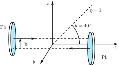
The direction of detected particles along the beam axis is given in terms of pseudo-rapidity $\eta$

$$\eta_{\text{pseudo}}\equiv\frac{1}{2}\ln\frac{|{\bf p}|+p_{z}}{|{\bf p}|-p_{z}}=-\ln\tan\frac{\theta}{2}$$ (2.3)

where $\theta$ is the angle from the beam axis and ${\bf p}$ is the momentum of a freely moving particle. Note that $\eta=1$ corresponds to $\theta\approx 40^{\circ}$ and $\eta=2.5$ to $\theta\approx 9.4^{\circ}$ (typical acceptance windows in a detector). When the mass of a particle can be neglected, $E\approx|{\bf p}|$, the pseudo-rapidity agrees with the particle momentum rapidity $y$ defined as

$$y_{\text{particle}}\equiv\frac{1}{2}\ln\frac{E+p_{z}}{E-p_{z}}.$$ (2.4)

The heavy ion collision picture known as the Bjorken expansion was a result of the important observation that the measured inclusive particle production is approximately flat in central rapidity $\eta\approx 0$ region [77], (see the current data in Fig. 2.4). The key assumption of this picture is that for the central rapidity region the system is boost invariant—system evolution and particle production looks the same in all reference frames related by a Lorentz boost in $z$-direction.

Figure 2.4: Approximately boost invariant measured charged particle multiplicity $dN_{\text{ch}}/d\eta$ in various centrality bins by (a) ATLAS [78] and (b) CMS [79] experiments.

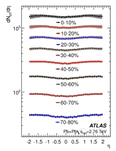
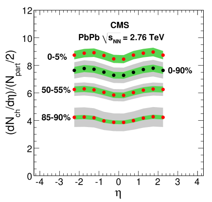
Such kinematics is best studied in the coordinates of “proper time” $\tau=\sqrt{t^{2}-z^{2}}$ and space-time rapidity

$$\eta_{\text{space-time}}\equiv\frac{1}{2}\ln\frac{t+z}{t-z}.$$ (2.5)

In $\tau\text{--}\eta$ coordinates, the (mostly positive) metric becomes

$$ds^{2}=-d\tau^{2}+dx^{2}+dy^{2}+\tau^{2}d\eta^{2}.$$ (2.6)

and boost-invariance in $z$ direction is equivalent to translational invariance in $\eta$ coordinate. The typical longitudinal momentum of produced particles is much larger than the transverse momentum $p^{z}\gg p_{\perp}$ and the subsequent expansion does not change the particle rapidity significantly. Since $p^{z}/E=v^{z}\approx z/t$ produced particles with momentum rapidity $y$ will reach the detector at space-time rapidity $\eta\approx y$.

Eqs. (2.3), (2.4), (2.5) define three different quantities: pseudo, particle and space-time rapidities, which are often used interchangeably when making estimates in heavy ion physics. Experimental results are given in pseudo-rapidity $\eta$, which directly relates to the detector coordinate system. Meanwhile simulations are often done using space-time rapidity $\eta$. The invariant mass of a pion—the most abundant species of detected hadrons—$m_{\pi}\approx 140\,{\rm MeV}$ is small compared to the typically measured energy of pions with transverse momentum $p_{\perp}\sim 1\,\text{GeV}$. Therefore massless pion approximation is adequate and indeed all three types of rapidities are approximately equal [80]

$$\eta_{\text{pseudo}}\approx y_{\pi}\approx\eta_{\text{space-time}}.$$ (2.7)

In the subsequent discussion we will not make a distinction between different types of rapidity and use the boost invariant picture of heavy ion collisions.

2.2.2 Initial conditions

One of the least understood stages in heavy ion collisions is the period between the passing of two nuclei and the formation of approximately equilibrated plasma around $\tau\sim 1\,\text{fm}$ [81]. The first principle QCD calculation of heavy ion nucleus wavefunction is not yet possible and a number of different models are used to describe the collision process [82].

Two nuclei collide when they pass each other at distance $|\mathbf{b}|\lesssim 2R_{\text{rms}}$, where $R_{\text{rms}}\sim 5\,\text{fm}$ is the root mean squared charge radius of a Pb nucleus (see Fig. 2.5(a)) [83].

Figure 2.5: Event plane view of the colliding nucleons along the beam axis. (a) The “almond shaped” overlap region (generally impact parameter $\mathbf{b}$ is randomly oriented in the transverse plane). (b) Monte Carlo Glauber sampled nucleon positions of participant nucleons (dark colored circles) and spectators (light colored circles) (Figure adapted from Ref. [84]).

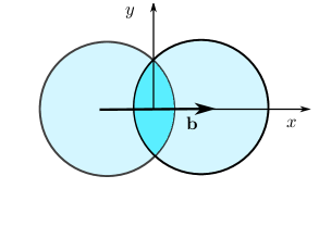
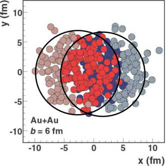
Current heavy ion collision models are based on a picture of a heavy ion nucleus composed of nucleons, whose positions are randomly distributed according to the average nuclear charge density function and subject to certain physical constrains, e.g. nucleons can not overlap due to nucleon-nucleon repulsion (see Fig. 2.5(b) for an example of nucleon positions sampled according to a popular Monte Carlo Glauber (MCG) procedure) [84, 85, 86]. At the LHC energies the two nuclei pass each other almost instantaneously $\Delta t_{\text{passing}}\sim 2R_{\text{Pb}}/(c\gamma)\sim 0.01\,\text{fm}$. Furthermore, the longitudinal boost of the nucleus is much larger than the intrinsic energy scale $\Lambda_{\text{QCD}}\sim 200\,\text{MeV}$ inside a nucleus and the transverse nuclear dynamics can be neglected. Then the nucleons appear frozen in the transverse plane during the passage and travel on straight lines along the beam axis [84, 80].

The principal difference between numerous initial state models (MCG, MCKLN, MCrcBK, IP-Glasma, EKRT) is in their treatment of which nucleons collide and how energy is deposited in the collision region [82]. The nucleons which do interact are called wounded nucleons or participants, while the remaining undeflected nucleons are known as spectators. Interaction between participant nucleons results in the extended energy deposition in the rapidity direction, from which the Quark Gluon Plasma is created. In the popular Monte Carlo Glauber model colliding nucleons are treated like spherical balls, which collide with one or more nucleons from the other nucleus if they are less than one diameter $D$ away in the transverse plane

$$D=\sqrt{\sigma_{NN}/\pi}\sim 1.5\,\text{fm}.$$ (2.8)

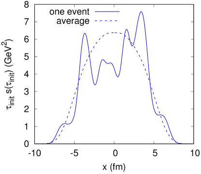
Here $\sigma_{NN}$ is a nucleon-nucleon inelastic cross-section obtained from p+p collision experiments [84]. When wounded nucleons are identified, one has to decide on energy or entropy deposition in the event. The equilibration process of colliding nucleons is highly nontrivial and largely unsolved problem [71, 32, 70], but essential features of the process can be efficiently parametrized by a handful of quantities and then fitted to reproduce the measured yields of particles [87, 88]. According to the two-component model used in simulations in Chapter 3, a lump amount of entropy density per rapidity is deposited in the transverse plane for each participant nucleon with adjustments for multiple binary collisions. This energy density distribution (example shown in Fig. 2.6) is then passed to the subsequent hydrodynamic evolution at time $\tau_{\text{init}}\sim 0.6\,\text{fm}$.

Figure 2.6: A typical entropy density profile (times ${\tau_{\rm init}}\sim 0.6\,\text{fm}$) for a single event used as an initial condition in current hydrodynamic simulations at the LHC for a 0-5% centrality class [1]. An event averaged initial condition is shown by the dashed line.

A considerable success of heavy ion simulations using MC Glauber initial conditions indicates that, indeed, the wounded nucleon distribution in the transverse collision area is the main source of variance in the collision [56, 89]. A more microscopic description of the early stages of hadron collisions can be obtained using the idea of Color Glass Condensate (CGC) [90, 91, 92, 93, 94, 95], which is motivated by the precision data from the DESY Hadron-Electron Ring Accelerator (HERA) [96]. At large collision energies the central rapidity region is dominated by the interactions of small Bjorken-$x$ partons (mostly gluons). The small $x$ gluons are produced (long before the collision) by highly boosted valence color charges, which evolve at much longer time scales and appear frozen, i.e. like Color Glass. Gluon density saturates at very high values $\rho\sim 1/\alpha_{s}\gg 1$, when gluon fusion becomes as favorable as collinear emission. Such high density gluons can be described as classical fields governed by Yang-Mills equations of motion [97]. The classical field evolution describes the energy liberation from the color currents, but does not lead to equilibrium and cannot be smoothly matched to hydrodynamic evolution [98, 99]. In Chapter 4 we use effective kinetic theory described in Sec. 2.2.8 to construct a practical implementation of the “bottom-up” thermalization scenario matching CGC initial conditions to hydrodynamics  [100, 70]. However, even without the precise description of equilibration, heavy ion collision simulations using CGC initial conditions show improvements over MC Glauber initial conditions for some observables, e.g. probability distribution of the magnitude of flow harmonics [65].

In Chapter 3 we use hydrodynamic heavy ion simulations with MC Glauber initial conditions, while in Chapter 4 we study the equilibration of CGC inspired initial state gluon distribution function.

2.2.3 Transverse geometry and spatial anisotropies

The transverse collision geometry is the dominant source of variance in heavy ion collisions and its description is of paramount importance for the interpretation of many experimental observables [66, 67].

It is customary to classify heavy ion collisions by their multiplicity—the number of produced charged particles (pions, kaons and protons) in each event [78, 79, 101]. For the small impact parameter $|\mathbf{b}|$, i.e. central (or head on) collision, the number of interacting nucleons is large and such collisions are likely to produce more particles. Conversely, the collisions at large $|\mathbf{b}|$ are peripheral and low in multiplicity. However, centrality does not completely fix the initial geometry configuration due to fluctuating number of participants even at a fixed impact parameter. Nevertheless, comparing central, mid-central and peripheral centrality bins allows one to study the effects of average background geometry.

The positions of wounded nucleons (few tens to four hundred) are the most import ingredients in determining the initial transverse energy distribution in the collision. Note that because of the finite number of wounded nucleons, participant distribution does not need to align with the overlap of average nuclear density illustrated in Fig. 2.5(a) and thus the collision geometry fluctuates on event-by-event basis as shown in Fig. 2.5(b) [56]. These event-by-event fluctuations in the transverse geometry are typically characterized by a series of eccentricity coefficients $\varepsilon_{n,m}$ defined in the center of mass frame as [66, 67]

$$\varepsilon_{n,m}e^{in\Phi_{n,m}} \equiv-\frac{[r^{m}e^{in\phi}]}{[r^{m}]}.$$ (2.9)

Here index $n$ is the order of the azimuthal harmonic $e^{in\phi}$, $m$ is the power of the radial weight $r^{m}$, and phase angle $\Phi_{n,m}$ (defined modulo ${2\pi}/{n}$) indicates the orientation of the particular azimuthal anisotropy relatively to the impact parameter $\mathbf{b}$. For example, the elliptic eccentricity given by Eq. (2.2) corresponds to the case $n=m=2$ and $\Phi_{2,2}=0$, i.e. the situation illustrated in Fig. 2.1(a).

Eccentricity is not experimentally measurable quantity and the precise way of computing them differs among authors, so brackets $[\ldots]$ can denote averaging with respect to either transverse energy or entropy density. Often the normalization factor $[r^{m}]$ is computed event-by-event together with the nominator to ensure that eccentricities are bounded above, $|\varepsilon_{n,m}e^{in\Phi_{n,m}}|<1$. In Chapter 3, we deviate from the common practice and use eccentricities defined in terms of transverse entropy distribution with event-class averaged normalization $R_{\rm rms}^{m}$.

On average, peripheral collisions have an “almond shaped” overlap, therefore $\varepsilon_{2,2}$, characterizing the elliptical deformation of collision geometry (see Fig. 2.5(a)), is the dominant eccentricity in all but the most central collisions. During the QGP expansion geometric anisotropies $\varepsilon_{n}$ are converted to momentum anisotropies $v_{n}$ of detected particles. A conventional minus sign in the eccentricity definition, Eq. (2.9), is chosen for a positive correlation between the two types of anisotropies. Thanks to event-by-event fluctuations, many other eccentricities can be excited, but the subsequent dissipative evolution of QGP suppresses higher harmonics [57, 58].

In Chapter 3 we show that standard eccentricities alone, given by Eq. (2.9), are not sufficient to capture all relevant information about the initial geometry and generalized eccentricities have to be considered to improve the correlation between the initial geometry and final momentum anisotropies.

2.2.4 Hydrodynamics

Significant momentum anisotropies $v_{n}$ of the observed particle spectrum in heavy ion collisions are strongly suggestive of the collective hydrodynamic motion in the expanding QGP fireball [102]. Indeed, phenomenological models have been remarkably successful in describing many soft observables and generally predicts the hydrodynamic phase to last from $\tau\sim 1\,\text{fm}$ to $\tau\sim 10\,\text{fm}$ [66, 75, 67, 68, 76].

Hydrodynamics is the long wavelength effective theory based on fundamental conservation laws of energy and momentum [103]

$$D_{\mu}T^{\mu\nu}=0,$$ (2.10)

where $D_{\mu}$ is the covariant derivative. The simplifying assumption of hydrodynamics is that $T^{\mu\nu}$ is a function of only four independent fields: the rest-frame energy density $e$ and the time-like flow velocity $u^{\mu}$ ($u^{\nu}u_{\nu}=-1$), satisfying

$$T^{\mu\nu}u_{\nu}=-eu^{\mu}.$$ (2.11)

The system of equations, Eq. (2.10), is closed by specifying the constitutive equations for the energy momentum tensor $T^{\mu\nu}(e({\bm{x}}),u^{\mu}({\bm{x}}))$, which for the smooth background fields can be systematically expanded in gradients

$$T^{\mu\nu}(e,u^{\mu})=T^{\mu\nu}_{\text{ideal}}+T^{\mu\nu}_{\text{1st order}}(\partial e,\partial u^{\mu})+T^{\mu\nu}_{\text{2nd order}}(\partial^{2}e,\partial^{2}u^{\mu})+\mathcal{O}(\partial^{3}).$$ (2.12)

Then truncation at the $n$th order in gradients defines the $n$th order hydrodynamics.

Ideal

The zeroth order truncation gives the ideal energy momentum tensor

$$T^{\mu\nu}_{\text{ideal}}=eu^{\mu}u^{\nu}+p\Delta^{\mu\nu},$$ (2.13)

where $\Delta^{\mu\nu}=g^{\mu\nu}+u^{\mu}u^{\nu}$ is the projection operator orthogonal to $u^{\nu}$ and $p$ is the pressure given by the equation of state $p=P(e)$ (see Sec. 2.2.5). At high temperatures $T\gg T_{c}\sim 155\,\text{MeV}$, QGP is often approximated as a gas of massless particles with constant speed of sound $c_{s}^{2}\equiv\partial p/\partial e={1}/{3}$, i.e. $p=c_{s}^{2}e$.

Using Eqs. (2.10) and (2.13) it is easy to show that the ideal equations of motion for energy density $e$ and flow velocity $u^{\mu}$ are

$$De=-(e+p)\theta,\quad Du^{\mu}=-\frac{\nabla^{\nu}p}{(e+p)},$$ (2.14)

with the following covariant notation

$$D\equiv u^{\mu}D_{\mu},\quad\nabla_{\mu}\equiv\Delta_{\mu}^{\phantom{\mu}\nu}D_{\nu},\quad\theta\equiv D_{\mu}u^{\mu}.$$ (2.15)

An important translationally invariant solution of Eq. (2.14) in $\tau\text{--}\eta$ coordinates is the Bjorken flow. It corresponds to a stationary fluid, where $u^{\tau}=1$ and $\theta\equiv D_{\mu}u^{\mu}={\tau^{-1}}$. The energy density $e$ then obeys

$$\partial_{\tau}e=-\frac{e+p}{\tau}$$ (2.16)

and $e\propto\tau^{-1-c_{s}^{2}}$ for $c_{s}^{2}=\text{const}$.

Navier-Stokes

Despite the initial success of ideal hydrodynamics in heavy ion collisions, it was recognized that there are viscous corrections which contributes at first order in gradients [53, 52, 51]. The only tensor structures built from energy and velocity gradients consistent with symmetries and Eq. (2.11) are

$$T^{\mu\nu}_{\text{1st order}}(\partial e,\partial u^{\mu})=\Pi\Delta^{\mu\nu}+\pi^{\mu\nu}.$$ (2.17)

where $\Pi(\partial e,\partial u^{\mu})$ is a scalar and $\pi^{\mu\nu}(\partial e,\partial u^{\mu})$ is a symmetric, traceless and $u^{\mu}$-orthogonal tensor [104]. The lower order equations of motion, Eqs. (2.14), can be used to replace energy gradients $\partial e$ with gradients in velocity $\partial u^{\mu}$. Then the first order viscous corrections are determined uniquely up to the overall coefficient

$$\Pi=-\zeta\theta,\quad\pi^{\mu\nu}=-\eta\sigma^{\mu\nu},$$ (2.18)

where $\sigma^{\mu\nu}$ is expressed in velocity gradients $D^{\mu}u^{\nu}$

$$\sigma^{\mu\nu}=2\left<D^{\mu}u^{\nu}\right>\equiv\Delta^{\mu\alpha}\Delta^{\nu\beta}(D_{\alpha}u_{\beta}+D_{\beta}u_{\alpha})-\frac{2}{3}\Delta^{\mu\nu}\Delta^{\alpha\beta}D_{\alpha}u_{\beta}.$$ (2.19)

Transport coefficients $\zeta$ and $\eta$ are called bulk and shear viscosity respectively and are of great interest in heavy ion collision physics. The effective constant shear viscosity is found to be in the range $1\lesssim 4\pi\eta/s\lesssim 3\text{--}6$ [105, 106], and quite close to the so called quantum bound of $\eta/s=1/(4\pi)\approx 0.08$. Constraining the temperature dependence of $\eta/s$ is an ongoing work [107]. Bulk viscosity $\zeta$ is expected to be small and perhaps become relevant close to the QCD transition temperature $T_{c}\sim 155\,\text{MeV}$ [108, 109, 110]. Therefore $\zeta$ is often neglected in hydrodynamic simulations of heavy ion collisions (but see, for example, [111]).

Second order

The dispersion relation $\omega(k)$ of relativistic Navier-Stokes equations predicts superluminal propagation of large wavenumber $k$ modes [112]. To render the equations of motion causal, the shear stress tensor $\pi^{\mu\nu}$ is promoted to a dynamical field, and the first order constitutive equations, Eq. (2.18), are imposed through a relaxation type equation [113]

$$\partial_{\tau}\pi^{\mu\nu}\sim-\frac{1}{\tau_{\pi}}(\pi^{\mu\nu}+\eta\sigma^{\mu\nu}).$$ (2.20)

This is equivalent to modifying constituent equations at second order in gradients. In conformal field theories in flat space-time there are only four such independent gradient structures [114]

$$T^{\mu\nu}_{\text{2nd order}} =\eta\tau_{\pi}\left[\left<D\sigma^{\mu\nu}\right>+\frac{1}{3}\sigma^{\mu\nu}\theta\right]+\lambda_{1}\left<\sigma_{\phantom{\mu}\lambda}^{\mu}\sigma^{\nu\lambda}\right>+\lambda_{2}\left<\sigma_{\phantom{\mu}\lambda}^{\mu}\Omega^{\nu\lambda}\right>+\lambda_{3}\left<\Omega_{\phantom{\mu}\lambda}^{\mu}\Omega^{\nu\lambda}\right>$$ (2.21)

and four second order transport coefficients $\tau_{\pi},\lambda_{1},\lambda_{2}$ and $\lambda_{3}$. Here $\Omega^{\mu\nu}$ stands for vorticity tensor

$$\Omega^{\mu\nu}=\frac{1}{2}\Delta^{\mu\alpha}\Delta^{\nu\beta}(\Delta_{\alpha}u_{\beta}-\Delta_{\beta}u_{\alpha}).$$ (2.22)

For strongly coupled $\mathcal{N}=4$ supersymmetric Yang Mills theory the second order transport coefficients can be calculated analytically [114, 115]

$$\frac{\tau_{\pi}}{\eta/(sT)}=4-\ln 4,\quad\frac{\lambda_{1}}{\tau_{\pi}\eta}=\frac{1}{2-\ln 2},\quad\frac{\lambda_{2}}{\tau_{\pi}\eta}=-\frac{\ln 4}{2-\ln 2},\quad\frac{\lambda_{3}}{\tau_{\pi}\eta}=0,$$ (2.23)

where the shear viscosity over entropy ratio saturates the quantum bound $\eta/s=1/(4\pi)$.

Using $\pi^{\mu\nu}=-\eta\sigma^{\mu\nu}$ in Eq. (2.21) one obtains a dynamical equation for the shear-stress tensor $\pi^{\mu\nu}$

$$\pi^{\mu\nu} =-\eta\sigma^{\mu\nu}-\tau_{\pi}\left[\left<D\pi^{\mu\nu}\right>+\frac{4}{3}\pi^{\mu\nu}\theta\right]-\frac{\lambda_{1}}{\eta}\left<\pi_{\phantom{\mu}\lambda}^{\mu}\sigma^{\nu\lambda}\right>-\frac{\lambda_{2}}{\eta}\left<\pi_{\phantom{\mu}\lambda}^{\mu}\Omega^{\nu\lambda}\right>+\lambda_{3}\left<\Omega_{\phantom{\mu}\lambda}^{\mu}\Omega^{\nu\lambda}\right>.$$ (2.24)

Then $e$, $u^{\mu}$ and five independent components of $\pi^{\mu\nu}$ are evolved according to Eqs. (2.10) and (2.24). For studies concerning observables at the central rapidity region (as it is the case in this manuscript), one often assumes boost invariance along the $z$-direction. Then dependence on rapidity $\eta$ coordinate is dropped, reducing the problem to the so called 2+1D hydrodynamics.

In Chapter 3 we perform hydrodynamic simulations using second order conformal hydrodynamic equations of motion Eqs. (2.10) and (2.24) with $\eta/s=1/(4\pi)$ and second order transport coefficients given in Eq. (2.23), but we employ non-conformal lattice equation of state (see Sec. 2.2.5). In Chapter 5 for the analytic calculations we use Navier-Stokes equations with constant speed of sound $c_{s}^{2}=1/3$.

2.2.5 Equation of state

Figure 2.7: (a) State of the art lattice equation of state at zero chemical potential. Figure taken from Ref. [116] (b) A sketch of QCD phase diagram as a function of temperature $T$ and baryon chemical potential $\mu_{B}$. The dashed line indicates a smooth crossover between hadronic and QGP phases, the solid line—a conjectured first order transition with second order critical end point (CEP). Figure taken from Ref. [29].

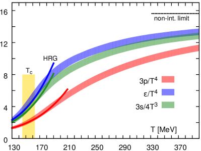
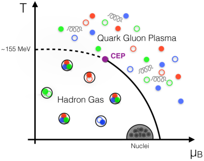
One necessary ingredient for the hydrodynamic description of heavy ion collisions is the relation between energy density $e$, baryon chemical potential $\mu_{B}$ and pressure $p$, i.e. the equation of state $p=p(e,\mu_{B})$. Thanks to the enormous computational effort, the first principle calculations of the equation of state are available from Lattice QCD [29]. Because of the famous sign problem for $\mu_{B}>0$, lattice computations are typically done at zero chemical potential. For high energy collisions the initial baryon number is negligible compared to the total produced number of particle-antiparticle pairs, therefore $\mu_{B}\approx 0$ is a reasonable approximation.

At temperatures below the deconfinement temperature $T_{c}\sim 155\,\text{MeV}$, the main degrees of freedom of the QCD are hadrons and a hadron resonance gas (HRG) model agrees well with the low temperature behavior of lattice equation of state (see Fig. 2.7(a)). At temperatures much higher than the deconfinement temperature $T_{c}$, the system is better described in terms of weakly interacting quarks and gluons and the equation of state is not too far from the massless gas limit. Lattice computations show that at zero chemical potential the transition between the two phases is a smooth crossover [117]. However, for $\mu_{B}>0$ one can have a first order phase transition line, which terminates at the critical end point (CEP) [118] (see Fig. 2.7(b)). This part of the phase diagram is accessible at medium energy nuclear collisions and is the target of the Beam Energy Scan program at RHIC [119, 120].

In Chapter 3, we use hydrodynamic equations derived in the conformal limit, but with lattice equation of state (s95p-v1 parametrization from Ref. [121]). The effective kinetic theory of Chapter 4 treats the QGP as a gas of weakly interacting massless particles, which automatically leads to a conformal equation of state $p=e/3$. For the sake of simplicity, the conformal equation of state is also used in semi-analytical computations of Chapter 5.

2.2.6 Freeze-out

In heavy ion collisions the QGP phase exists only for $\tau\sim 10\,\text{fm}$ before evaporating into hadrons, and it is only the long lived particles (pions, kaons and protons) which are eventually detected [122]. Transition from the deconfined quarks and gluons to the hadronic degrees of freedom is described by a freeze-out procedure.

When the plasma temperate falls below the pseudo-critical temperature $T_{c}\sim 155\,\text{MeV}$, gluons and quarks recombines into hadrons (pions being the most abundant species). The change in the degrees of freedom is reflected in the rapid crossover of the equations of state (see Fig. 2.7(a)). As the system continues to expand and cool down, the hadronic rescatterings are not sufficiently rapid to keep the system in local equilibrium. The macroscopic hydrodynamic description has to be replaced with microscopic kinetic theory evolution of hadrons until all interactions and decays terminate.

The transition to kinetic description is typically done at a constant temperature $T_{\text{fo}}\sim T_{c}$, where all particle species are assumed to be in chemical and thermal equilibrium. Then the particle distribution functions is given by the Cooper-Frye formula [123]

$$E\frac{d^{3}N_{s}}{d^{3}p}=\frac{\nu_{s}}{(2\pi)^{3}}\int_{\sigma}f_{s}(x^{\nu},p^{\nu})p^{\mu}d\sigma_{\mu},$$ (2.25)

where $\sigma$ is the freeze-out surface ($T=T_{\text{fo}}$) and $f_{s}(\mathbf{x},{\bf p})$ is the distribution function for particle species $s$ produced by a fluid cell moving with velocity $u^{\nu}$. In ideal fluid dynamics, one simply takes boosted equilibrium distribution $f_{s}(\mathbf{x},{\bf p})=f_{\text{eq}}(-u^{\nu}p_{\nu}/T)$, but in a dissipative fluid the distribution function $f_{s}$ acquires viscous corrections [124].

The subsequent kinetic evolution of hadrons can be done in hadronic transport models, e.g. UrQMD [125]. In practice the kinetic interactions does not modify the pion spectrum significantly therefore in qualitative (and even quantitative) studies only the freeze-out spectrum, Eq. (2.25), is used to estimate the observed flow harmonics [126, 127, 88].

In Chapter 3 we use the pion freeze-out spectrum at $T_{\text{fo}}=140\,\text{MeV}$ to estimate the flow harmonics at the end of hydrodynamic evolution.

2.2.7 Momentum anisotropies

In each heavy ion collision event thousands of particles are detected over several units of pseudo-rapidity $\eta$ and azimuthal angle $\varphi$. Particles can be further binned by species and the transverse momentum $p_{T}$ they carry. Particles with energy well above QGP temperature, i.e. $p_{T}\gtrsim 5\,\text{GeV}$, are produced at the initial instant of the heavy ion collision and are the source of the jet phenomena [128, 129]. High energy parton jets interact with the QGP medium, but are generally not considered part of it. Meanwhile soft momentum particles $p_{T}\lesssim 5\,\text{GeV}$ are shown to exhibit collective behavior characteristic of an equilibrated medium evolving as a whole [66, 75, 67, 68, 76]. In this work we will concentrate on the properties of the medium and will not discuss the high $p_{T}$-physics.

The key consequence of considering QGP as a locally equilibrated medium is that particles are produced according to some underlying probability distribution in $p_{T},\eta$ and $\varphi$ [130]

$$E\frac{d^{3}N}{d^{3}p}=\frac{d^{3}N}{p_{T}dp_{T}d\eta d\phi}$$ (2.26)

and each event is a finite realization of this distribution. However, each collision happens at a random impact parameter $\mathbf{b}$ (both the size and the orientation of $\mathbf{b}$ can fluctuate). Therefore events are classified in centrality bins ($\sim|\mathbf{b}|$), while the event plane angle ($\sim$ orientation of $\mathbf{b}$) is estimated from the measured particles (or observables are constructed in such a way that they do not depend on the event plane angle).

In the QGP medium paradigm, all soft-physics information about the event is contained in the particle distribution function and accurate computation of the distribution function is the principal goal of heavy ion collision simulations [67]. Similarly, experimentalists try to determine the underlying distribution function from heavy ion collision measurements and separate it from the high-$p_{T}$ physics [130]. In the rest of this section we will define several observables on which theory to experiment comparisons are typically performed, and which play an important role in Chapter 3.

Theory definitions

At rest a thermalized medium produces particles isotropically in the azimuthal angle $\varphi$. However, the non-isotropic expansion of the QGP fireball introduces azimuthal anisotropies in the particle spectrum known as flows, which are studied using the azimuthal Fourier series of particle distribution function [131, 130]

$$E\frac{d^{3}N}{d^{3}p}=\frac{d^{2}N}{2\pi p_{T}dp_{T}d\eta}\left(1+2\sum_{n=1}^{\infty}v_{n}(p_{T},\eta)\cos n(\varphi-\Psi_{n}(p_{T},\eta))\right).$$ (2.27)

Here particle distribution function is expressed in terms of azimuthally averaged particle yield ${d^{2}N}/{2\pi p_{T}dp_{T}d\eta}$ and Fourier coefficients $v_{n}(p_{T},\eta)$—flow harmonics. The azimuthal angle $\Psi_{n}(p_{T},\eta)$ defines the orientation of the particular anisotropy in the transverse plane. The index $n$ labels the order of Fourier harmonics and only the first few terms are significant and have associated terminology

$$n=1 \quad\text{directed flow},$$ (2.28)

$$n=2 \quad\text{elliptic flow},$$ (2.29)

$$n=3 \quad\text{triangular flow},$$ (2.30)

$$n=4 \quad\text{quadrangular flow},$$ (2.31)

$$n=5 \quad\text{pentagonal flow}.$$ (2.32)

The $n=0$ Fourier coefficient is normalized to one in Eq. (2.27), but it is by far the largest Fourier component of the underlying distribution function and is called the radial flow.

When boost invariant picture of heavy ion collisions is applicable (the case assumed throughout this manuscript), the rapidity dependence can be dropped or integrated over in Eq. (2.27). Furthermore, it is also often assumed that the orientation of a particular flow component in the transverse plane, $\Psi_{n}$, is $p_{T}$ independent [67]. Then

$$\frac{1}{\Delta\eta}\int_{\eta_{\text{min}}}^{\eta_{\text{max}}}\!\!d\eta\,E\frac{d^{3}N}{d^{3}p}=\frac{dN}{2\pi p_{T}dp_{T}}\left(1+2\sum_{n=1}^{\infty}v_{n}(p_{T})\cos n(\varphi-\Psi_{n})\right),$$ (2.33)

and the momentum dependent $v_{n}(p_{T})$ flow vector has momentum independent orientation $\Psi_{n}$ in the azimuthal plane. In Chapter 3 we show that this particular assumption does not hold exactly due to the existence of subleadings flows. Finally, a single number characterizing the strength of harmonic flow in a collision is the momentum integrated $v_{n}$

$$\frac{dN}{d\varphi}\propto 1+2\sum_{n=1}^{\infty}v_{n}\cos n(\varphi-\Psi_{n}),$$ (2.34)

where $dN/d\varphi$ is particle yield over all rapidity $\eta$ and momentum $p_{T}$ bins.

Experimental definitions

Theoretically it is simpler to start with the most differential observable, Eq. (2.27), and then narrow down to integrated quantities, Eq. (2.34). In the experiment, however, the finite number of measured particles in each event makes differential observables the most challenging ones to measure [130]. On the other hand, the integrated $v_{n}$ in a single event can be estimated by averaging over all detected particles

$$v_{n}^{\text{obs}}e^{in\Psi_{n}^{\text{obs}}}=\left<e^{in\varphi}\right>.$$ (2.35)

This estimated value $v_{n}^{\text{obs}}$ fluctuates event-by-event around the true value $v_{n}$, but can be corrected through a number of methods [130]. The number of particles in one event is not sufficient to have an accurate estimate of more differential flow observables, instead one uses the large number of similar events to do the event average. For example, the event-plane method uses the orientation of the integrated $v_{n}$, Eq. (2.35), to calculate the differential momentum anisotropy in the $v_{n}$ plane [67, 130]

$$v_{n}(p_{T})=\left<\cos(n(\varphi(p_{T})-\Psi_{n})\right>.$$ (2.36)

Such measurement does not depend on the random orientation of the impact parameter $\mathbf{b}$ in the lab frame (see Fig. 2.3) and can be safely averaged over many different events.

An alternative method of extracting the underlying distribution function is to look at pair correlations in the collision [67, 130]

$$v_{n\Delta}(p_{T1},p_{T2})=\left<\left<e^{in(\varphi_{1}-\varphi_{2})}\right>\right>_{\text{events}},$$ (2.37)

where $\varphi_{1}$ and $\varphi_{2}$ are azimuthal angles of two separate particles with momentum $p_{T1}$ and $p_{T2}$ respectively in the same event. The two-particle angular correlation is clearly independent of the collision orientation.

The equilibrated medium emits particles independently, thus for one event the pair production yield factorizes into single particle distribution functions

$$\frac{d^{6}N_{\text{pairs}}}{d^{3}p_{1}d^{3}p_{2}}=\frac{d^{3}N}{d^{3}p_{1}}\frac{d^{3}N}{d^{3}p_{2}}+\mathcal{O}(N).$$ (2.38)

The factorizable term scales with the particle number as $\mathcal{O}(N^{2})$ and is the source of so called collective or flow correlations. The second term denotes the non-flow correlations, which have typical $\mathcal{O}(N)$ scaling. These are the correlations that are not collective for the entire medium, e.g. resonance decay chain, Bose-Einstein correlation, etc. The non-flow correlations are usually narrow in rapidity $\eta$, therefore they can be further suppressed by imposing pseudo-rapidity gaps between the correlated particles [130]. We will neglect the non-flow contributions in further discussion.

Substituting single particle distribution function Eq. (2.27) in the pair production yield formula Eq. (2.38) and taking the average over events results in the following relation between the two-particle and the single particle Fourier components

$$v_{n\Delta}(p_{T1},p_{T2})\equiv\left<\left<e^{in(\varphi_{n1}-\varphi_{n2})}\right>\right>_{\text{events}}=\left<v_{n}(p_{T1})v_{n}(p_{T2})\cos{n(\Psi_{n1}-\Psi_{n2})}\right>_{\text{events}}$$ (2.39)

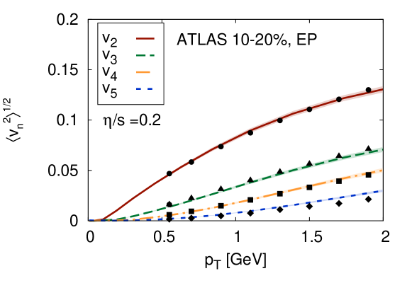
The correlation matrix on the left is experimentally measurable and encodes information about the single particle distribution function. For instance, the diagonal of the correlation matrix gives the root-mean-square of the harmonic flow $v_{n}(p_{T})$

$$v_{n}\{2\}(p_{T})\equiv v_{n\Delta}(p_{T},p_{T})=\sqrt{\left<v_{n}(p_{T})^{2}\right>}.$$ (2.40)

The rms harmonic flow vectors is well reproduced by hydrodynamic simulations of heavy ion collisions and agrees with experimental measurements as shown in Fig. 2.8.

Figure 2.8: Comparison of rms anisotropic flow coefficients $\left<v_{n}^{2}\right>^{1/2}$ as a function of transverse momentum in hydrodynamic simulation and experimental data [60]. Figure taken from Ref. [65].

If the flow angle $\Psi_{n}$ is independent of momentum $p_{T}$ and there are no event-by-event fluctuations in flow magnitude $v_{n}(p_{T})$, then the right hand side of Eq. (2.39) factorizes

$$v_{n\Delta}(p_{T1},p_{T2})=v_{n}(p_{T1})\times v_{n}(p_{T2}).$$ (2.41)

Such flow factorization can be experimentally tested by measuring the factorization ratio

$$r_{n}(p_{T1},p_{T2})=\frac{v_{n\Delta}(p_{T1},p_{T2})}{\sqrt{v_{n\Delta}(p_{T1},p_{T1})v_{n\Delta}(p_{T2},p_{T2})}}.$$ (2.42)

Experimental measurements show that at ${\sqrt{s_{\scriptscriptstyle NN}}}=2.76\,\text{TeV}$ Pb+Pb collisions factorization is broken [132, 133, 134]. In particular, for the second harmonic flow $v_{2}$ factorization breaking reaches $\sim 20\%$ for the most central Pb+Pb, but is small in peripheral collisions (see Fig. 2.9).

Figure 2.9: Factorization ratio, $r_{2}$, as a function of transverse momentum difference $p_{T}^{a}-p_{T}^{b}$ in bins of $p_{T}^{a}$ for Pb+Pb collisions at ${\sqrt{s_{\scriptscriptstyle NN}}}=2.76\,\text{TeV}$. Figure taken from Ref. [132].

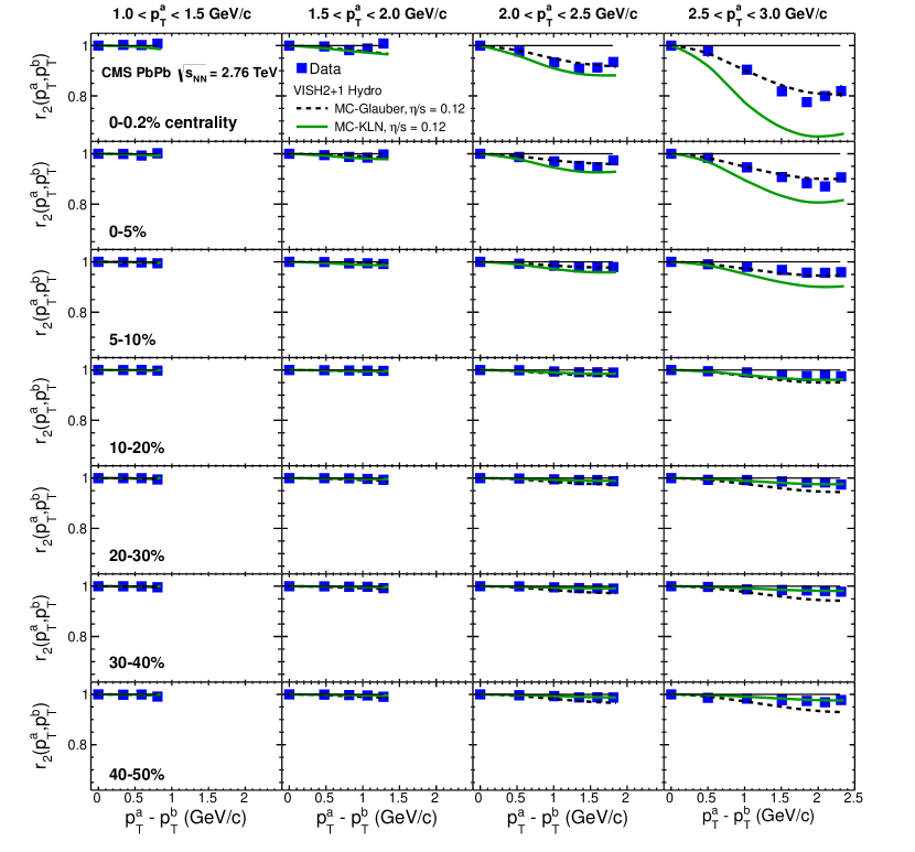
Initially, factorization breaking was interpreted as a sign of non-flow effects, but later it was understood that even in purely hydrodynamic models initial fluctuations will cause factorization breaking [135]. Studying the entire two-particle correlations matrix, Eq. (2.39), or factorization ratio, Eq. (2.42), provides an access to initial fluctuations not captured by the integrated flow observables.

In Chapter 3 we use Principal Component Analysis to decompose the two-particle correlations, Eq. (2.39), into the most significant components for boost invariant hydrodynamic simulations at ${\sqrt{s_{\scriptscriptstyle NN}}}=2.76\,\text{TeV}$. We show how principal components can be used to describe and interpret the transverse momentum factorization breaking.

2.2.8 QCD medium at high temperature

One of remarkable properties of the QCD is the running of the coupling constant $\alpha_{s}=g^{2}/(4\pi)$. At large collision energies, the coupling appears small and the hard cross-sections can be calculated using leading order QCD diagrams in vacuum [14, 15, 17]. Indeed, many calculations for proton-proton collisions based on the Standard Model compares excellently against the experimental measurements [136]. The increased collision energy of heavy ion collisions at LHC (from ${\sqrt{s_{\scriptscriptstyle NN}}}=200\,\text{GeV}$ at RHIC to ${\sqrt{s_{\scriptscriptstyle NN}}}=2.76\,\text{GeV}$ and ${\sqrt{s_{\scriptscriptstyle NN}}}=5.02\,\text{GeV}$ at LHC) allows creation of matter with initial temperature 2-4 times above the QCD transition temperature $T_{c}\sim 155\,\text{MeV}$ [137]. Therefore the bulk dynamics of the early stages of the collision might be described by the perturbative processes of high temperature QCD [138].

QCD processes in a medium are more complicated than those in vacuum, because a naive diagrammatic expansion in coupling constant fails to correctly account for all contributing processes at the same order in $g$, as clarified by Braaten and Pisarski [139]. For a systematic treatment of such contributions, one needs a separation of scales. At weak coupling $g\ll 1$ and high temperature $T\gg T_{c}$ , the QGP is energetically dominated by high energy quasi-particles with typical (hard) momentum $p\sim T$. Loop corrections to the free propagator create an effective thermal mass $m_{\text{th}}\sim gT$ which is much smaller than the hard particle energy scale $p\sim T$, therefore hard partons can be treated as nearly massless excitations of the plasma traveling in $\sim gT$ background. Over times much longer than duration of any scattering process, hard particles can be described by an effective kinetic theory; the phase space density $f({\bm{x}},{\bf p})$ of hard particles then obeys a Boltzmann equation,

$$(\partial_{t}+\mathbf{v}\cdot\mathbf{\nabla}_{x})f=-C[f],$$ (2.43)

where $|\mathbf{v}|=1$ and $C[f]$ is the collision kernel. The leading order effective kinetic theory of high temperature gauge theories was laid out in the seminal paper by Arnold, Moore and Yaffe [140], and is known as the AMY formalism.

Figure 2.10: (a) Hard elastic $2\rightarrow 2$ scattering with $\sim T$ momentum exchange (b) Soft elastic $2\rightarrow 2$ scattering with medium regulated $m_{\text{th}}\sim gT$ propagator (c) Collinear splitting of hard quasi-particle into two hard particles due to soft $\sim gT$ momentum exchange with the medium.

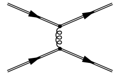
At leading order the hard parton dynamics is governed by elastic $2\leftrightarrow 2$ scatterings and inelastic $1\leftrightarrow 2$ particle number changing QCD bremsstrahlung. When two hard partons exchange $\mathcal{O}(T)$ momentum, they undergo a large angle $\theta\sim 1$ scattering with a rate $\sim g^{4}T$ (see Fig. 2.10(a)). For a soft momentum exchange (small scattering angle), the cross-section is quadratically divergent in vacuum, but in the medium it is regulated by a thermal mass $m_{\text{th}}\sim gT$ (diagram Fig. 2.10(b)). Therefore small angle scatterings $\theta\sim g$ occur at a rate $\sim g^{2}T$, i.e. much more often than large angle scatterings, but the cumulative diffusive effect is of the same order as a single hard scattering. In addition to elastic scatterings, hard quasi-particles can split into two near collinear hard particles thanks to soft momentum $\sim gT$ exchange with the medium (see Fig. 2.10(c)). Such radiative process is prohibited by energy-momentum conservation in vacuum and is crucial to the equilibration of the ultra-relativistic plasma [100, 141]. The perturbed hard parton has small virtuality and travels distance $\sim(g^{2}T)^{-1}$ before splitting. During this time multiple soft scatterings can occur and the destructive interference between different scattering events leads to suppression of collinear splitting known as the Landau-Pomeranchuk-Migdal (LPM) effect. Fully resummed leading order effective $1\leftrightarrow 2$ scattering rate can be obtained from an integral-differential equation [142].

Figure 2.11: Strong coupling constant $\alpha_{s}(Q)$ as a function of energy scale $Q$. Figure taken from Ref. [16]

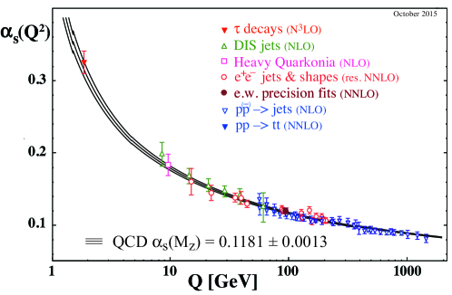
With all leading order terms correctly accounted for, the kinetic theory provides an effective description of high temperature QCD medium and can be used to calculate, for example, the transport properties of the medium [143]. The AMY formulation of the effective kinetic theory has a number of requirements [140]:

• The temperature $T$ is sufficiently high that the coupling constant is small $g\ll 1$ and all other QCD scales (quark masses and $\Lambda_{QCD}$) are negligible compared to the thermal masses $m_{\text{th}}\sim gT$.

• The system is sufficiently close to local thermal equilibrium, which is defined by slowly varying local temperature $T({\bm{x}})$ and velocity $u^{\mu}({\bm{x}})$ fields

  $$f({\bm{x}},{\bf p})=n(|{\bf p}|;T({\bm{x}}),u^{\mu}({\bm{x}}))+\delta f({\bm{x}},{\bf p}),\quad\delta f\ll f$$ (2.44)

  where $n(|{\bf p}|;T,u^{\mu})$ is an equilibrium (Bose or Fermi) distribution.

As can be seen from Fig. 2.11, the running of the coupling constant $\alpha_{s}$ is slow and $g=\sqrt{4\pi\alpha_{s}}$ is never parametrically small in the accessible energy range. Consequently, “hard” $\sim T$ and “soft” $\sim gT$ momentum scales are not widely separated and the soft sector contributions have to be calculated non-perturbatively [144]. Modern perturbative theory techniques were shown to reproduce various thermodynamic quantities for $T>2\text{--}3T_{c}$ [145, 146] and there is a considerable progress of extending dynamical calculations of effective kinetic theory beyond the leading order [147]. Therefore applying the leading order AMY kinetic theory at realistic values of the coupling constant $\alpha_{s}\sim 0.3$ in heavy ion collisions is an extrapolation from the weak coupling regime, but it is built on first principle systematically improvable calculations with single parameter—the coupling constant.

At the initial moments after the collision, the QGP is believed to be in highly anisotropic state with longitudinal pressure $P_{L}$ much smaller than the transverse pressure $P_{T}$ [98, 99]. In AMY formulation of the kinetic theory the distribution function is restricted to parametrically small anisotropies, because of Weibel instability [148, 149]. The origin of Weibel instability is that charged particles respond differently to magnetic field perturbations depending on their direction of motion. In isotropic plasma the positive and negative feedbacks cancel out, but if the particle distribution function is anisotropic, certain field perturbations will be reinforced leading to an instability. However, in the QCD the self interaction between the soft modes slows down the exponential growth of the instability and classical lattice simulations show that plasma instabilities are not important beyond the transient time [150, 99, 98, 151, 152]. This motivates applying isotropically screened kinetic theory even to systems with considerable anisotropy. However, the applicability of effective kinetic theory could be considerably widened if anisotropic screening would be taken into account non-perturbatively [153, 154, 155].

In Chapter 4 we use leading order effective kinetic theory with isotropic screening to model isotropization of gluon distribution function at realistic values of the coupling constant $\alpha_{s}\approx 0.26$.

2.3 Outline

2.3.1 Chapter 3: Principal Component Analysis

Problem

The evolution of heavy ion collisions is a highly non-trivial map between initial conditions and observables. Thanks to small QGP viscosity, many imprints of the initial state features can be seen in the measured particle spectrum. The observed flow factorization breaking (see Fig. 2.9 and Sec. 2.2.7) can be explained by flow angle and magnitude decorrelations with the transverse momentum [135, 156, 157], indicating that that there are multiple independent sources of harmonic flow in heavy ion collisions. These subleading flows are a response to different features of the initial geometry, and therefore their combined contribution to $v_{n}$ cannot be predicted by a single geometrical quantity like $\varepsilon_{n}$. Only by correctly identifying the generating sources for all subleading flows, one can fully understand the map between initial conditions and final state observables.

Idea

To disentangle the separate causes of flow, one can use the full information contained in the two-particle correlation matrix, Eq. (2.39). A simple statistical method to achieve that is Principal Component Analysis (PCA) [158, 159]. Given a $N\times N$ covariance matrix of $N$ observables, PCA identifies the largest statistically uncorrelated sources of variance in the system. This greatly reduces the dimensionality of the problem. Instead of the full $N\times N$ covariance matrix, one can deal with just few dominant principal components. Schematically, event-by-event harmonic flow $v_{n}(p_{T})$ can be written as a sum of leading principal components

$$v_{n}(p_{T})e^{in\Psi_{n}(p_{T})}\propto\xi_{1}v_{n}^{(1)}(p_{T})+\xi_{2}v_{n}^{(2)}(p_{T})+\ldots$$ (2.45)

where $\xi_{1}$ and $\xi_{2}$ are complex coefficients encoding angle and magnitude fluctuations of leading and subleading principal components. PCA guarantees that different components are statistically uncorrelated, i.e.

$$\left<\xi_{i}\xi_{j}^{*}\right>=\delta_{ij}$$ (2.46)

and that (real) principal component vectors $v_{n}^{(a)}(p_{T})$ are mutually orthogonal with a certain measure $w(p_{T})$, which has to be specified

$$\int dp_{T}w(p_{T})v_{n}^{(a)}(p_{T})v_{n}^{(b)}(p_{T})\propto\delta^{ab}.$$ (2.47)

The weight function $w(p_{T})$ can be chosen to maximize the difference between physically independent sources of momentum dependent harmonic flow $v_{n}(p_{T})$. However, if the response has the same momentum dependence, one needs additional information to differentiate between flow sources. Since we are interested in collective flow, we weigh each momentum bin by corresponding multiplicity, thus giving the largest weight to correlations involving the largest number of particles. Therefore our choice for the weight function is

$$w(p_{T})=\left(\frac{dN}{2\pi p_{T}dp_{T}}\right)^{2},$$ (2.48)

but other choices are also possible. The weight function can be absorbed by defining multiplicity weighted harmonic flow

$$V_{n}^{(a)}(p_{T})\equiv v_{n}^{(a)}(p_{T})\times\frac{dN}{2\pi p_{T}dp_{T}}.$$ (2.49)

With this definition $V_{n}$ flow is proportional to the observed particle count and is analogous to the experimentally measured $Q_{n}$ vector [130]. Then the multiplicity weighted two-particle correlation function can be efficiently expanded in terms of principal components. For elliptic flow

Figure 2.12: Factorization ratio $r_{2}(p_{T1},p_{T2})$ [Eq. (2.51)] for elliptic flow and its approximations with principal components (PCs) in hydrodynamical simulations of central (0–5%) and peripheral (45–50%) collisions.

$$\big{<}V_{2,p_{T1}}V^{*}_{2,p_{T2}}\big{>}=V_{2}^{(1)}(p_{T1})V^{(1)}_{2}(p_{T2})+V_{2}^{(2)}(p_{T1})V^{(2)}_{2}(p_{T2})+\ldots.$$ (2.50)

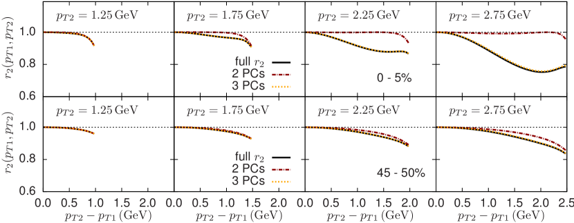
Just two or three terms are needed to give an excellent approximation of the full factorization ratio $r_{2}(p_{T1},p_{T2})$ defined now as

$$r_{2}(p_{T1},p_{T2})\equiv\frac{\left\langle V_{2}(p_{T1})V_{2}^{*}(p_{T2})\right\rangle}{\sqrt{\left\langle|V_{2}(p_{T1})|^{2}\right\rangle\left\langle|V_{2}(p_{T2})|^{2}\right\rangle}}\,.$$ (2.51)

In Fig. 2.12 we see that indeed principal components efficiently describe factorization ratio in hydrodynamical simulations, which can be compared with experimentally measurements in Fig. 2.9.

Application

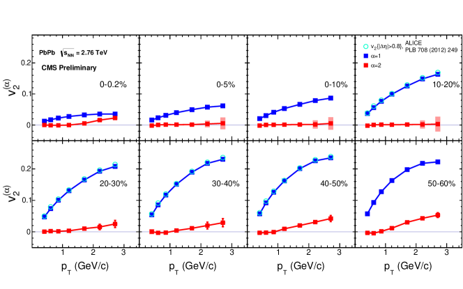
Principal Component Analysis is a systematic way of expressing harmonic flow in statistically uncorrelated components. Because principal components are typically strongly ordered, only the leading two or three components are sufficient to describe factorization breaking [160]. In Chapter 3, we demonstrate that each component can be given an intuitive physical interpretation as a hydrodynamic response to particular initial state features (radial excitations of eccentricities) or a nonlinear response to the lower order harmonic flow. The first phenomenological application of PCA in studying factorization breaking in heavy ion collisions was introduced in [160, 1], which was followed by the first experimental measurements of principal components for elliptic and triangular flow in Pb+Pb and p+Pb collisions in Ref. [161]. As can be seen from the experimental results shown in Fig. 2.13, the subleading elliptic flow is significant in peripheral and ultra-central collisions, which is consistent with findings in our work. However the subleading principal component for triangular flow was found to be negligible for Pb+Pb collisions at ${\sqrt{s_{\scriptscriptstyle NN}}}=2.76\,\text{TeV}$ [161].

Figure 2.13: First and second principal component for elliptic flow as a function of $p_{T}$ in different centrality bins for Pb+Pb collisions at ${\sqrt{s_{\scriptscriptstyle NN}}}=2.76\,\text{TeV}$. Figure taken from Ref. [161].

Another area of applications for PCA is the factorization breaking in pseudo-rapidity $\eta$ [132, 60, 162]. Here the flow decorrelation at different rapidity bins was associated with forward-backward asymmetric in nuclear collisions [163, 164, 165]. The $\eta$ dependent flow or multiplicity can be decomposed in terms of orthogonal polynomials [164, 166] or principal components as an optimal basis [160]. Analogously to the case of transverse momentum correlations, principal component analysis presents itself as a data driven method of utilizing all information of the two particle correlations function.

In Chapter 3 we present a comprehensive Principal Component Analysis for flow harmonics $n=0\text{--}5$ in boost invariant hydrodynamic simulations of heavy ion collisions at ${\sqrt{s_{\scriptscriptstyle NN}}}=2.76\,\text{TeV}$.

2.3.2 Chapter 4: Weak coupling equilibration

Problem

The process of equilibration in heavy ion collisions is currently a hotly debated topic [69, 70, 32, 71]. Conventionally, for hydrodynamics to be applicable, one needs an approximate local thermal equilibrium or at least pressure isotropization [167], but phenomenological simulations use relativistic second order hydrodynamics at times as early as $\tau=0.2\,\text{fm}$, when pressure anisotropies are still large [65, 168]. This naturally leads to a question of how QGP approaches hydrodynamic behavior in such a short time. In addition, the initial out-of-equilibrium evolution determines the starting conditions for hydrodynamics, which is one of the main sources of uncertainty in the extraction of QGP transport coefficients [105, 106]. A clear understanding of pre-equilibrium dynamics is necessary to have a consistent picture of heavy ion collisions and can be crucial in interpreting signals of collectivity in small collisions systems like p+Pb and p+p.

Idea

At asymptotically high temperatures, but moderate densities, the QGP can be viewed as a gas of weakly coupled particles with effective kinetic description, which is also applicable out-of-equilibrium. By following the evolution of these hard partons in kinetic theory, one can understand the equilibration from the first principle QCD calculations. For heavy ion collisions such “bottom-up” path to thermalization in weakly coupled QCD was laid out in the seminal paper by Baier, Mueller, Schiff and Son [100]. The paper assumes the Color Glass Condensate (CGC) picture of the initial state of heavy ion collision, which is characterized by large saturation scale $Q_{s}\gg\Lambda_{QCD}$, parametrically high density $f\sim\alpha_{s}^{-1}$ and strongly interactions (despite the coupling constant $\alpha_{s}\ll 1$ being small). By the time $\tau Q_{s}>1$ the longitudinal expansion dilutes the system sufficiently that it can be described as a collection of quasi-particles with well defined, but highly anisotropic distribution function $f({\bm{x}},{\bf p})$. Most of energy is carried by hard $p\sim Q_{s}$ gluons, which undergo elastic $2\leftrightarrow 2$ scatterings, but thanks to longitudinal expansion the anisotropy continues to grow. Eventually the number density of hard gluons drops below one and they start cascading to the soft sector through collinear splitting. The soft gluons (relatively to the saturation scale $Q_{s}$) collide often and quickly thermalize. The remaining hard partons loose their energy to this thermal bath and the system reaches equilibrium.

Figure 2.14: Kinetic theory describes the evolution from the microscopic formation time $\tau_{0}$ to the equilibration time $\tau_{\text{init}}$, when hydrodynamics becomes applicable [70]. By causality, for a given point in the transverse plane it is sufficient to analyze the pre-equilibrium evolution within the causal neighborhood of that point.

Another important aspect of the pre-thermal evolution for heavy ion collision is the propagation of initial fluctuations in the transverse plane (see Fig. 2.14). In weak coupling framework the different stages of thermalization are parametrically separated by the inverse powers of the coupling constant $\alpha_{s}\ll 1$ and the kinetic theory describes the evolution of the system from the microscopic formation time $\tau_{0}\sim Q_{s}^{-1}$ to the (much later) times when hydrodynamics becomes applicable $\tau_{\text{init}}\sim\tau_{\text{equilibrium}}$ [70]. In practice (and for realistic values of the coupling constant $\alpha_{s}\approx 0.26$ in kinetic theory [169]), the hydrodynamization time is short, $\tau_{\text{init}}\sim 1\,\text{fm}$, and initial perturbations interact locally. In other words, for a given point ${\bm{x}}_{0}$ in the transverse plane the causally connected region $|{\bm{x}}-{\bm{x}}_{0}|\leq c(\tau_{\text{init}}-\tau_{0})\sim 1\,\text{fm}$ is much smaller than the total transverse nuclear geometry $R_{\text{Pb}}\sim 5\,\text{fm}$, but comparable to a single nucleon scale $R_{p}\sim 1\,\text{fm}$. Therefore heavy ion collisions evolution from $\tau_{0}$ to $\tau_{\text{init}}$ can be decomposed into equilibration of translationally invariant background and small perturbations around it in the causally connected region $|{\bm{x}}-{\bm{x}}_{0}|\leq c(\tau_{\text{init}}-\tau_{0})$ (see Fig. 2.14). For linear perturbations the pre-equilibrium evolution can be conveniently expressed in terms of Green functions, which map initial perturbations to energy momentum tensor at the times when hydrodynamics is applicable. By convolving kinetic theory response functions with microscopic initial state models like IP-Glasma, we can obtain initial conditions for hydrodynamics with the complete pre-thermal evolution history.

Application

The early time dynamics in heavy ion collisions is under active investigations in both strong coupling holographic approach in model theories [32] and weak coupling framework in QCD [71]. Realistic collisions happen in neither of these idealized limits, but both can be used as physically motivated bounds for the equilibration in heavy ion collisions [170]. Recent work on classical Yang-Mills evolution [99, 98], showed that the “bottom-up” scenario [100] is the preferred thermalization picture in a weak coupling framework. It was put to practice for uniform boost invariant background in Ref. [169], showing that kinetic theory (extrapolated to realistic values of the coupling constant $\alpha_{s}\approx 0.26$) describes equilibration and approach to hydrodynamics in phenomenologically feasible, i.e. short enough, time. In Chapter 4 we extend this work to include the equilibration of transverse perturbations and demonstrate that they too hydrodynamize.

One of the goals of early time dynamics is to complement the successful hydrodynamic simulations of heavy ion collisions with the complete pre-equilibrium evolution. Various approaches taken include continuing classical Yang-Mills evolution [171], using free streaming [172, 173], taking holography inspired initial conditions [174, 175, 70] or different formulations of hydrodynamics [176]. The main advantages of kinetic theory equilibration are that it is based on the first principle QCD and automatically leads isotropization and approach to hydrodynamics. Kinetic theory is also a natural continuation of the successful microscopic initial state models based on CGC framework.

In Chapter 4 we use effective kinetic theory to construct Green functions for the linearized perturbations around boost invariant background and demonstrate equilibration and hydrodynamization of CGC inspired out-of-equilibrium initial conditions.

2.3.3 Chapter 5: Non-equilibrium thermal fluctuations

Problem

Since fluctuations in heavy ion collisions is one of the main tools of inferring medium properties, understanding the various sources of fluctuations is central to heavy ion physics. A considerable effort went into modeling the creation and propagation of initial state fluctuations, e.g. second order hydrodynamics or IP-Glasma initial conditions. However, the QGP (as any dissipative medium) must also have thermal fluctuations [177, 178]. Ordinarily, such fluctuations are suppressed by the large number of constituents, but a QGP droplet is on the edge of what can be called a macroscopic system with of order $\sim 10^{4}$ of produced particles [78, 79]. Secondly, thermal fluctuations have been long known to create long time tails $\propto t^{-\frac{3}{2}}$ in the two point correlation functions [179, 180, 181]. Formally such fractional power terms break the gradient expansion of relativistic hydrodynamics at the second order [182] and therefore a consistent higher order description of heavy ion collisions needs to assess the nonlinear noise contributions. Finally, the discovery of the QGP opened up a completely new domain in the phase diagram of hot and dense nuclear matter. Naturally, chartering out this new territory requires determining the transition line between the QGP and ordinary hadronic matter. At high collision energies, i.e. small baryon chemical potential, lattice computations indicate a smooth transition between the two phases, however at $\mu_{B}>0$ a first order transition is possible [118]. The ongoing Beam Energy Scan (BES) program at RHIC is aimed to find the signs of the first order transition and the critical end point—the point where smooth crossover turns into the first order transition. Critical points in the phase diagrams are characterized by and dominated by stochastic fluctuations [177]. Therefore thermal fluctuations must be an important ingredient in the correct interpretation of the experimental signatures of the critical point.

Idea

Any system in thermal equilibrium at temperature $T$ must satisfy fluctuation-dissipation theorem, which in frequency space $\omega$ is

$$G_{S}(\omega)=\frac{2T}{\omega}\text{Im}\,G_{R}(\omega),$$ (2.52)

where $G_{S}(\omega)$ is symmetrized correlator capturing the magnitude of fluctuations and $G_{R}(\omega)$ is the retarded Green function describing system response to perturbations [177]. Microscopically the meaning of fluctuation-dissipation theorem is that a dissipative system can loose energy only to the microscopic degrees of freedom, however in equilibrium, the opposite process must occur and microscopic degrees of freedom induces macroscopic thermal fluctuations in the system.

Hydrodynamics is an effective theory describing long wavelength physics $\lambda\gg l_{\text{mfp}}$, where $l_{\text{mfp}}$ is microscopic medium scale, e.g. mean free path. The medium properties like rest frame energy density $e$ and pressure $p$ is the manifestation of kinetic and potential energy contained in the microscopic degrees of freedom. Similarly, transport coefficients like viscosity $\eta$ characterize the energy transfer from modes with $\lambda>l_{\text{mfp}}$ to those below the hydrodynamic cut-off, $\lambda<l_{\text{mfp}}$. The hydrodynamics discussed in Sec. 2.2.4 does not include thermal fluctuations, however it is well known how to incorporate stochastic terms in hydrodynamic equations of motion [177, 178] (for a recent review see [104])

$$D_{\mu}T^{\mu\nu}=0,\quad T^{\mu\nu}=T^{\mu\nu}_{\text{ideal}}+T^{\mu\nu}_{\text{visc.}}+S^{\mu\nu},$$ (2.53)

where $S^{\mu\nu}$ is a noise term with zero mean, and variance $\left\langle S^{\mu\nu}S^{\rho\sigma}\right\rangle{\sim}2T\eta\delta(t-t^{\prime})$. Solving hydrodynamics with noise gives the complete energy density and velocity evolution for all wavelengths $\lambda>l_{\text{mfp}}$, for which Eq. (2.53) is valid, but the solution is not deterministic and depends on the stochastic noise. Short wavelength fluctuations make numerical simulations very challenging and one is typically interested in the average noise effect to the long wavelength physics. Averaging Eq. (2.53) over noise gives an effective equation of motion for physical perturbations over length scales much larger than the dominant distances of noise

$$D_{\mu}\left<T^{\mu\nu}(e,u^{\sigma})\right>=0.$$ (2.54)

Figure 2.15: The hydro-kinetic description of noise is based on the separation of scales between the long wavelength hydrodynamic background (with $k\sim\omega/c_{s}$), and shorter wavelength hydrodynamic fluctuations (with $k\sim k_{*}\equiv\sqrt{\omega/\gamma_{\eta}}$). The wavelengths of the hydrodynamic fluctuations are still much longer than microscopic mean free path. The hydrodynamic fluctuations are driven out of equilibrium by the expanding background, and this deviation is the origin of the long-time tail correction to the stress tensor.

Energy momentum tensor is a non-linear function in background fields $e$ and $u^{\sigma}$, therefore expanding $T^{\mu\nu}$ around the averaged fields gives

$$\left<T^{\mu\nu}(e,u^{\sigma})\right>=T^{\mu\nu}(\left<e\right>,\left<u^{\sigma}\right>)+\mathcal{O}(\left<v^{i}v^{j}\right>)\ldots$$ (2.55)

As we see fluctuations modify the background constitutive equations by the quadratic contributions from two point correlation functions $N^{ij}\sim\left<v^{i}v^{j}\right>$. In equilibrium such terms can be calculated using thermal correlation functions and it amounts to a constant renormalization of background energy and transport coefficients. Rest frame energy density renormalization can be simply understood as including kinetic energy of noise fluctuations in the average energy density. After the appropriate redefinition of background fields and transport coefficients ordinary hydrodynamic equations can be solved.

The situation is different in systems where the evolution, characterized by frequency $\omega$, is fast enough to drive hydrodynamic fluctuations out of equilibrium. The dissipative relaxation timescale of modes with wavenumber $k$ is given by $\gamma_{\eta}k^{2}$, where $\gamma_{\eta}=\eta/(e+p)$ is the momentum diffusion coefficient. Balance between the driving frequency and relaxation rate

$$\omega\sim\gamma_{\eta}k_{*}^{2}$$ (2.56)

defines a dissipative scale $k_{*}$ separating the long wavelength physics at $\omega/c_{s}$ and short wavenumber hydrodynamic fluctuations, which remain in equilibrium (see Fig. 2.15)

$$\frac{\omega}{c_{s}}\ll k_{*}\ll\frac{1}{l_{\text{mfp}}}.$$ (2.57)

Importantly, out-of-equilibrium hydrodynamic fluctuations at $k\sim k_{*}$ obey the known hydrodynamic equations of motion, Eq. (2.53), and we show that by using the separation of scales given by Eq. (2.57) it is possible to derive hydro-kinetic equations for expectation of two point correlation functions $N^{ij}\sim\left<v^{i}v^{j}\right>$ for $k\sim k_{*}$

$$\partial_{\tau}N=-\underbrace{Dk^{2}(N-N_{0})}_{\text{relaxation to equilibrium}}+\underbrace{FN}_{\text{forcing}}.$$ (2.58)

Deviations of a stationary solution of Eq. (2.58) from the equilibrium value $N_{0}$ around the dissipative scale $k_{*}$ determines modifications to the nonlinear noise contributions in Eq. (2.55), which is the principal outcome of hydrodynamics with noise.

Application

Thermal fluctuations occur naturally in dissipative systems, but in the context of heavy ion collisions hydrodynamic fluctuations have been considered only recently [183, 182]. The direct dependence of thermal noise on the medium parameters makes hydrodynamic fluctuations an attractive alternative probe of viscous coefficients in QGP. Previous calculations considered one dimensional averaged noise effects for the expanding Bjorken flow [184, 185] and numerical simulations of hydrodynamics with noise on smooth [186, 187, 188] and event-by-event fluctuating backgrounds [189]. The short range of noise correlations makes it problematic to simulate noise correctly on numerical grids. Instead in Chapter 5 we propose effective hydro-kinetic equations, which can be in principle coupled to existing hydrodynamic simulations to determine the nonlinear noise contributions to the relevant long wavelength physics. In the framework of hydro-kinetics, the 3D momentum phase space of hydrodynamic fluctuations can be straightforwardly organized to give a physically intuitive interpretation of different noise effects. Finally, the hydro-kinetics is not restricted to close-to-equilibrium systems and can be applied to general hydrodynamic backgrounds.

In Chapter 5 we derive effective hydro-kinetic equations for noise correlations in the expanding Bjorken background and calculate the nonlinear noise modifications of background constitutive equations.

Chapter 3 Subleading flows and factorization breaking with principal components

The material in the following sections previously appeared in:

• A. Mazeliauskas and D. Teaney, Subleading harmonic flows in hydrodynamic simulations of heavy ion collisions, Phys. Rev. C91, 044902 (2015) [1]. Copyright (2015) by the American Physical Society

• A. Mazeliauskas and D. Teaney, Fluctuations of harmonic and radial flow in heavy ion collisions with principal components, Phys. Rev. C93, 024913 (2016) [2], Copyright (2016) by the American Physical Society

3.1 Introduction

Two-particle correlation measurements are of paramount importance in studying ultra-relativistic heavy ion collisions, and provide an extraordinarily stringent test for theoretical models. Indeed, the measured two-particle correlations exhibit elliptic, triangular, and higher harmonics flows, which can be used to constrain the transport properties of the quark gluon plasma (QGP) [66, 67]. The remarkable precision of the experimental data as a function of transverse momentum and pseudorapidity has led to new analyses of factorization breaking, nonlinear mixing, event shape selection, and forward-backward fluctuations [132, 190, 191, 192, 193, 194]. In this paper we analyze the detailed structure of two-particle transverse momentum correlations by using event-by-event (boost-invariant) hydrodynamics and principal component analysis (PCA) [160]. Specifically, we decompose the event-by-event harmonic flow $V_{n}(p_{T})$ into principal components and investigate the physical origin of each of these fluctuations. Here we present an extensive theoretical study of $n=0\text{--}5$ flow harmonics at the LHC (Pb+Pb at ${\sqrt{s_{\scriptscriptstyle NN}}}=2.76\,{\rm TeV}$) . In particular, we demonstrate the importance of radial flow fluctuations for subleading flows of higher harmonics.

Taking the second harmonic for definiteness, the two-particle correlation matrix of momentum dependent elliptic flows, $C_{2}(p_{T1},p_{T2})\equiv\left\langle V_{2}(p_{T1})V_{2}^{*}(p_{T2})\right\rangle$ is traditionally parametrized by factorization ratio $r_{2}(p_{T1},p_{T2})$ [135],

$$r_{2}(p_{T1},p_{T2})\equiv\frac{\left\langle V_{2}(p_{T1})V_{2}^{*}(p_{T2})\right\rangle}{\sqrt{\left\langle|V_{2}(p_{T1})|^{2}\right\rangle\left\langle|V_{2}(p_{T2})|^{2}\right\rangle}}\,.$$ (3.1)

If there is only one source of elliptic flow in the event [for example if in each event $V_{2}(p_{T})=f(p_{T})\varepsilon_{2}$ with $\varepsilon_{2}$ a complex eccentricity and $f(p_{T})$ a fixed real function of $p_{T}$] then the correlation matrix of elliptic flows $C_{2}(p_{T1},p_{T2})$ factorizes into a product of functions, and the $r_{2}$ parameter is unity. However, if there are multiple independent sources of elliptic flow in the event, then the correlation matrix does not factorize, and the $r_{2}$ parameter is less than unity [135]. The $r_{2}$ parameter has been extensively studied both experimentally [132, 134, 60, 162] and theoretically [135, 156, 157]. PCA is a statistical technique that decomposes the flow correlation matrix into eigenvectors and eigenvalues. The procedure naturally identifies the most important contributions to flow fluctuations. Typically only two or three modes are needed to give an excellent description of the full covariance matrix (see Fig. 3.1). When there are only two significant eigenvectors, the $r_{n}$ matrix can be expressed as [160]

$$r_{n}(p_{T1},p_{T2})\simeq 1-\frac{1}{2}\left(\frac{V_{n}^{(2)}(p_{T1})}{V_{n}^{(1)}(p_{T1})}-\frac{V_{n}^{(2)}(p_{T2})}{V_{n}^{(1)}(p_{T2})}\right)^{2}\,,$$ (3.2)

where $V_{n}^{(1)}(p_{T})$ and $V_{n}^{(2)}(p_{T})$ are the first and second eigenvectors. In particular, in the case of triangular flow, factorization breaking in event-by-event hydrodynamics arises because the simulated triangular flow is predominantly the result of two statistically uncorrelated contributions—the linear response to $\varepsilon_{3}$ [86] and the linear response to the first radial excitation of $\varepsilon_{3}$. The extension of this understanding of factorization breaking to the other harmonics was surprisingly subtle due to the quadratic mixing between the leading and subleading harmonic flows.

Experimentally, it is observed that factorization breaking is largest for elliptic flow in central collisions (see in particular Fig. 28 of Ref. [60] and Fig. 1 of Ref. [132]). Indeed, the $r_{2}$ parameter decreases rather dramatically from mid-central to central collisions. This indicates that the relative importance of the various initial state fluctuations which drive elliptic flow are changing rapidly as a function of centrality. The current manuscript explains the rapid centrality dependence of factorization breaking in $v_{2}$ as an interplay between the linear response to the fluctuating elliptic geometry, and the nonlinear mixing of the radial flow and average elliptic flow. This quadratic mixing is similar to the mixing between $v_{5}$ and $v_{2},v_{3}$  [195, 89, 196, 197], and this picture can be confirmed experimentally by measuring specific three point correlations analogous to the three plane correlations measured in the $v_{5},v_{2},v_{3}$ case [190, 191].

To understand the linear and nonlinear contributions quantitatively, we will break up the fluctuations in hydrodynamics into their principal components, and analyze the linear and nonlinear contributions of each principal component to the simulated harmonic spectrum. In Sects. 3.2 and 3.3 we review the analysis definitions, and the key features of simulations. To gain insight into the results of PCA analysis, we will first look at the leading and subleading harmonics of triangular flow (which is sourced entirely by fluctuations). Section 3.4 studies the basic properties of the subleading triangular flow, such as its dependence on centrality and viscosity. In Sec. 3.5 we show that the subleading triangular flow arises (predominantly) from the radial excitation of the triangular geometry. In Sec. 3.6 we discuss the strategy for constructing the best linear predictor for leading and subleading flows. We define a generalized eccentricity $\varepsilon_{n}\{\rho(r)\}$ in Eq. (3.26) and use radial Fourier modes to optimize the radial weight $\rho(r)$. The geometric predictors described above are ultimately based on the assumption of linear response. At least for the third harmonic, these assumptions are checked in Sec. 3.6.1.

After gaining experience with the triangular flow, we summarize the key results of a comprehensive principal component analysis of flow harmonics $n=0\text{--}5$ in the second part of our paper. In Sec. 3.7 we give individual discussions for each harmonic flow and construct optimal predictors for leading and subleading flows based on initial geometry and nonlinear mixing. First, we discuss radial flow fluctuations in Sec. 3.7.1 and then demonstrate their importance in generating subleading elliptic flow in Sec. 3.7.2. In Sec. 3.7.3 we describe our PCA results for direct and triangular flows. Finally, in Sec. 3.7.4 we discuss the quadrangular and pentagonal flows and how the nonlinear mixing of lower order principal components adds to these flows. We put forward some experimental observables in the discussion in Sec. 3.8. For convenience, we present a catalog of figures showing PCA results for each harmonic in the Appendix.

3.2 Principal components

PCA is a statistical technique for extracting the dominant components in fluctuating data. In the context of flow in heavy ion collisions it was first introduced in Ref. [160] to quantify the dominant momentum space fluctuations of harmonic flows in transverse momentum and rapidity in a precise way. This section provides a brief review of this statistical technique.

Paraphrasing Ref. [160], in the flow picture of heavy ion collisions the particles in each event are drawn independently from a single particle distribution which fluctuates from event to event. The event-by-event single particle distribution is expanded in a Fourier series

$$\frac{{d}N}{{d}{\bf p}}=V_{0}(p_{T})+\sum_{n=1}^{\infty}V_{n}(p_{T})e^{-in\varphi}+{\rm H.c.}\,,$$ (3.3)

where ${d}{\bf p}={d}y\,{d}p_{T}\,{d}\varphi$ notates the phase space, $\varphi$ is the azimuthal angle of the distribution, and H.c. denotes Hermitian conjugate. $V_{n}(p_{T})$ is a complex Fourier coefficient recording the magnitude and orientation of the $n$th harmonic flow. This definition deviates from the common practice of normalizing the complex Fourier coefficient by the multiplicity, $v_{n}(p_{T})=V_{n}(p_{T})/V_{0}(p_{T})$.

Up to non-flow corrections of order the multiplicity $N$, the long-range part of the two-particle correlation function is determined by the statistics of the event-by-event fluctuations of the single distribution

$$\left\langle\frac{{d}N_{\text{pairs}}}{{d}{\bf p}_{1}{d}{\bf p}_{2}}\right\rangle=\left\langle\frac{{d}N}{{d}{\bf p}_{1}}\frac{{d}N}{{d}{\bf p}_{2}}\right\rangle+\mathcal{O}\left(N\right)\,.$$ (3.4)

If the two-particle correlation function is also expanded in a Fourier series

$$\left\langle\frac{{d}N_{\text{pairs}}}{{d}{\bf p}_{1}{d}{\bf p}_{2}}\right\rangle=\sum_{n}V_{n\Delta}(p_{T1},p_{T2})e^{-in(\varphi_{1}-\varphi_{2})}\,,$$ (3.5)

then this series determines the statistics of $V_{n}(p_{T})$

$$C_{n}(p_{T1},p_{T2})\equiv V_{n\Delta}(p_{T1},p_{T2})-\left<V_{n,p_{T1}}\right>\left<V^{*}_{n,p_{T2}}\right>=\big{<}\big{(}V_{n,p_{T1}}-\left<V_{n,p_{T1}}\right>\big{)}\big{(}V^{*}_{n,p_{T2}}-\left<V^{*}_{n,p_{T2}}\right>\big{)}\big{>}\,.$$ (3.6)

The covariance matrix $C_{n}(p_{T1},p_{T2})$, which is real, symmetric, and positive-semidefinite, can be decomposed into real orthogonal eigenvectors $V_{n}^{(a)}(p_{T})$,

$$C_{n}(p_{T1},p_{T2})= \sum_{a}\lambda^{a}\psi^{(a)}_{n}(p_{T1})\psi^{(a)}_{n}(p_{T2})=\sum_{a}V_{n}^{(a)}(p_{T1})V^{(a)}_{n}(p_{T2}),$$ (3.7)

where $V_{n}^{(a)}(p_{T})\equiv\sqrt{\lambda^{a}}\,\psi^{(a)}_{n}(p_{T})$ is the square root of the eigenvalue times a normalized eigenvector $\int_{0}^{\infty}\!dp_{T}\,\psi^{(a)}\psi^{(b)}=\delta_{ab}$. The eigenvalue records the squared variance of a given fluctuation.

The principal components $V_{n}^{(1)}(p_{T}),V_{n}^{(2)}(p_{T}),\ldots$ of a given event ensemble can be used as optimal basis for event-by-event expansion of harmonic flow

$$V_{n}(p_{T})-\left<V_{n}(p_{T})\right>=\xi_{n}^{(1)}V^{(1)}_{n}(p_{T})+\xi_{n}^{(2)}V^{(2)}_{n}(p_{T})+\ldots\,.$$ (3.8)

The complex coefficients $\xi_{n}^{(a)}$ are the projections of harmonic flow onto principal component basis and record the orientation and event-by-event amplitude of their respective flows. Principal components are mutually uncorrelated

$$\left<\xi_{n}^{(a)}\xi_{n}^{*(b)}\right>=\delta^{ab}.$$ (3.9)

Typically the eigenvalues of $C_{n}(p_{T1},p_{T2})$ are strongly ordered and only the first few terms in the expansion are significant. Often the large components have a definite physical interpretation. We define the scaled magnitude of the flow vector $V_{n}^{(a)}(p_{T})$ as

$$\|v^{(a)}_{n}\|^{2}\equiv\frac{\int\big{(}V_{n}^{(a)}(p_{T})\big{)}^{2}dp_{T}}{\int\left<dN/dp_{T}\right>^{2}dp_{T}},$$ (3.10)

which is a measure of the size of the fluctuation without trivial dependencies on the mean multiplicity in a given centrality class.

Figure 3.1: Factorization ratio $r_{2}(p_{T1},p_{T2})$ [Eq. (3.11)] for elliptic flow and its approximations with principal components (PCs) in central (0–5%) and peripheral (45–50%) collisions.

The leading flow vector $V^{(1)}_{n}(p_{T})$ corresponds to fluctuations with the largest root-mean-square amplitude, while subsequent components maximize the variance in the remaining orthogonal directions. This yields a very efficient description of the full covariance matrix $C_{n}(p_{T1},p_{T2})$ and factorization ratio

$$r_{n}(p_{T1},p_{T2})\equiv\frac{C_{n}(p_{T1},p_{T2})}{\sqrt{C_{n}(p_{T1},p_{T1})C_{n}(p_{T2},p_{T2})}}\leq 1\,.$$ (3.11)

$r_{n}(p_{T1},p_{T2})$ is bounded by unity within hydrodynamics [135]. By truncating series expansion of the covariance matrix [Eq. (3.7)] at two or three principal components we can approximate $C_{n}(p_{T1},p_{T2})$ and $r_{n}(p_{T1},p_{T2})$. Truncating at the leading term would constitute complete flow factorization, i.e., $r_{n}=1$. The factorization matrix for elliptic flow is shown in Fig. 3.1. We see that in peripheral collisions at low momentum $p_{T}<2.5\,\rm{GeV}$ just two principal components are sufficient to describe momentum dependence of factorization ratio $r_{2}$. In central collisions (as explained in Sec. 3.7.2) the subleading and subsub-leading elliptic flows are comparable and both are needed to given an excellent description of $r_{2}$.

Analogous decompositions of two-particle correlations into principal components exist for all harmonics and all centralities. Interpreting these large flow components physically is the goal of this work.

3.3 Simulations

We used boost-invariant event-by-event viscous hydrodynamics to simulate 5000 Pb-Pb collisions at the CERN Large Hadron Collider (LHC) (${\sqrt{s_{\scriptscriptstyle NN}}}=2.76\,{\rm TeV}$) in fourteen 5% centrality classes selected by impact parameter. Our simulations are boost invariant and implement second order viscous hydrodynamics [114], using a code base which has been developed previously [126, 197]. For the initial conditions we use the Phobos Glauber Monte Carlo [86], and we distribute the entropy density in the transverse plane according to a two-component model. Specifically, for the $i$th participant we assign a weight

$$A_{i}\equiv\kappa\left[\frac{(1-\alpha)}{2}+\frac{\alpha}{2}(n_{\rm coll})_{i}\right]\,,$$ (3.12)

with $\alpha=0.11$, $\kappa=35.1$ for $\eta/s=0.08$, and $\kappa=32.8$ for $\eta/s=0.16$. $(n_{\rm coll})_{i}$ is the number of binary collisions experienced by the $i$th participant; so the total number of binary collisions is $N_{\rm coll}={\textstyle\frac{1}{2}}\sum_{i}(n_{\rm coll})_{i}$. The entropy density in the transverse plane at initial time $\tau_{o}$ and transverse position ${\bm{x}}=(x,y)$ is taken to be

$$s(\tau_{o},{\bm{x}})=\sum_{i\in{{N_{\rm parts}}}}s_{i}(\tau_{o},{\bm{x}}-{\bm{x}}_{i})\,,$$ (3.13)

where ${\bm{x}}_{i}=(x,y)$ labels the transverse coordinates of the $i_{\rm th}$ participant, and

$$s_{i}(\tau_{o},{\bm{x}})=A_{i}\,\frac{1}{\tau_{o}(2\pi\sigma^{2})}e^{-\frac{x^{2}}{2\sigma^{2}}-\frac{y^{2}}{2\sigma^{2}}}\,,$$ (3.14)

with $\sqrt{2}\sigma=0.7\,{\rm fm}$. The parameters $\kappa$ and $\alpha$ are marginally different from Qiu’s thesis [88], and we have independently verified that this choice of parameters reproduces the average multiplicity in the event.

The equation of state is motivated by lattice QCD calculations [198] and has been used previously by Romatschke and Luzum [199]. In this paper we compute “direct” pions (i.e. pions calculated directly from the freeze-out surface) and we do not include resonance decays. We use a freeze-out temperature of $T_{\rm fo}=140\,{\rm MeV}$.

Simulation results were generated for fourteen 5% centrality classes with impact parameter up to $b={12.4}\rm{fm}$ and at two viscosities, $\eta/s=0.08$ and $\eta/s=0.16$. Unless specified, the results are for $\eta/s=0.08$. We generated 5000 events per centrality class. We then performed PCA for the $n$th harmonic $V_{n}(p_{T})$ by discretizing $V_{n}(p_{T})$ results from hydrodynamics into 100 equally spaced bins between $p_{T}=0\ldots 5\,{\rm GeV}$, and finding the eigenvalues and eigenvectors of the resulting Hermitian matrix.

Table 3.1 records the Glauber data which is used in this analysis. Event-by-event averages with the initial entropy density are notated with square brackets, e.g.

$$[r^{2}]\equiv\frac{1}{\overline{S}_{\rm tot}}\int d^{2}{\bm{x}}\,\tau_{o}s(\tau_{o},{\bm{x}})r^{2},$$ (3.15)

where $\overline{S}_{\rm tot}$ is the average total entropy in a given centrality class, $\left<\int d^{2}{\bm{x}}\,\tau_{o}s(\tau_{o},{\bm{x}})\right>$. Averages over events are notated with $\left\langle\,\right\rangle$, so that the root mean square radius is

$$R_{\rm rms}\equiv\sqrt{\left<[r^{2}]\right>}\,.$$ (3.16)

As a technical note, here and below the radius is measured from the center of entropy, so $[{\bm{x}}]=0$. $\varepsilon_{n,m}$ is defined in a somewhat unorthodox fashion in Eq. (3.24), with $\varepsilon_{3,3}^{\rm rms}\equiv\sqrt{\left\langle|\varepsilon_{3,3}|^{2}\right\rangle}$. $\overline{r}_{\rm max}$ is the averaged maximum participant radius, ${\rm max}\,|{\bm{x}}_{i}|$.

Centrality	($b_{\rm min},b_{\rm max}$)	$\overline{N}_{\rm part}$	$R_{\rm rms}$	$\overline{r}_{\rm max}$	$\varepsilon_{3,3}^{\rm rms}$
0–5 %	(0.0,   3.3)	384	4.1	8.1	0.11
5–10 %	(3.3,   4.7)	335	3.9	7.8	0.14
10–15%	(4.7,   5.7)	290	3.7	7.5	0.17
15–20%	(5.7,   6.6)	250	3.6	7.3	0.20
20–25%	(6.6,   7.4)	215	3.4	7.0	0.22
25–30%	(7.4,   8.1)	184	3.3	6.7	0.25
30–35%	(8.1,   8.8)	156	3.2	6.4	0.28
35–40%	(8.8,   9.4)	132	3.1	6.2	0.32
40–45%	(9.4,   9.9)	110	3.0	5.9	0.35
45–50%	(9.9,   10.5)	91	2.9	5.7	0.39
50–55%	(10.5,  11.0)	74	2.7	5.4	0.44
55–60%	(11.0,  11.5)	60	2.7	5.1	0.48
60–65%	(11.5,  11.9)	47	2.6	4.8	0.52
65–70%	(11.9,  12.4)	37	2.4	4.4	0.55

Table 3.1: Table of parameters from the Glauber model (all distances are measured in fm).

3.4 Subleading triangular flow

To gain insight into principal components of harmonic flow, we first analyze triangular flow, since it is a strong signal and is driven entirely by fluctuations [56]. As a first step, we list the (scaled) magnitudes of flows $\|v_{3}^{(a)}\|$ [Eq. (3.10)] in central collisions for the simulations described above.

$a$	1	2	3	4
$\|v_{3}^{(a)}\|$	$1.5\times 10^{-2}$	$2.6\times 10^{-3}$	$4.8\times 10^{-4}$	$1.1\times 10^{-4}$

Note that the scaled magnitudes are proportional to the square-root of the eigenvalues, $\|v_{3}^{(a)}\|\propto\sqrt{\lambda_{a}}$. From the decreasing magnitudes of the listed (scaled) magnitudes, we see that the first two eigenmodes account for 99.9% of the squared variance, which can be represented as a sum of the eigenvalues

$$\int_{0}^{\infty}{d}p_{T}\left\langle V_{3}(p_{T})V_{3}^{*}(p_{T})\right\rangle= \sum_{a}\lambda_{a}\propto\sum_{a}\|v_{3}^{(a)}\|^{2}\,.$$ (3.17)

Figure 3.2(a) displays the eigenvectors, $V_{3}^{(a)}(p_{T})$, for the leading and first two subleading modes. We see that for triangular flow only the first two flow modes are significant. To make contact with the more traditional definitions of $v_{3}(p_{T})$, we divide by $\left\langle{d}N/{d}p_{T}\right\rangle$ and present the same eigenmodes in Fig. 3.2(b).

Figure 3.2: Momentum dependence of triangular flow components in central collisions. a) Principal flow vectors, $V^{(a)}_{3}(p_{T})$. b) Principal flow vectors divided by the average multiplicity, $v_{3}^{(a)}(p_{T})\equiv V_{3}^{(a)}(p_{T})/\left\langle{d}N/{d}p_{T}\right\rangle$.

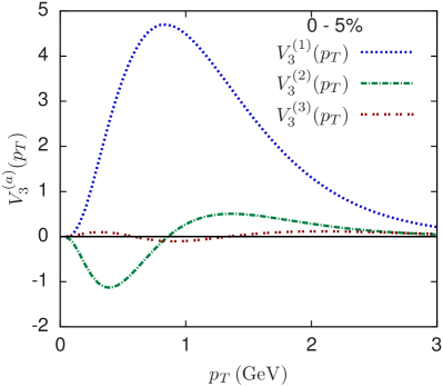
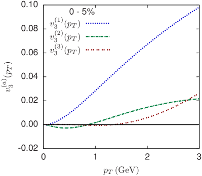
We also investigated the centrality and viscosity dependence of the principal components. The normalized principal flow eigenvectors $\psi^{(a)}_{3}(p_{T})$ are approximately independent of viscosity (not shown). In Fig. 3.3, we show the centrality dependence of these normalized eigenvectors. In more central collisions the eigenvectors shift to larger transverse momentum, which can be understood with the system size scaling introduced in Ref. [200].

Figure 3.3: Centrality dependence of triangular flow eigenvectors $\psi^{a}(p_{T})$.

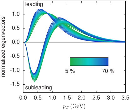
The magnitude of the flow, i.e. the squared integral $\int\,(V_{3}^{(a)}(p_{T}))^{2}dp_{T}$, depends on both centrality and viscosity. To factor out the trivial multiplicity dependence of $V_{3}(p_{T})$, we plot the scaled flow eigenvalues $\|v_{n}^{(a)}\|$ [see Eq. (3.10)] in Fig. 3.4. Going from $\eta/s=0.08$ to $\eta/s=0.16$ we see significant suppression of the leading mode. In general the subleading scaled flow $\|v_{3}^{(a)}\|$ depends weakly on centrality.

Figure 3.4: Centrality and viscosity dependence of scaled eigenvalues $\|v^{(a)}_{3}\|$. (The subleading flow has been magnified 5 times to bring to scale with leading flow.)

We present PCA results on all harmonic $n=0\text{--}5$ in the Appendix 3.A. Namely, we show the flow magnitude dependence on centrality for the largest three principal components, and principal eigenvectors in central 0-5% bin. Individual discussions for each harmonic are given in Sec. 3.7.

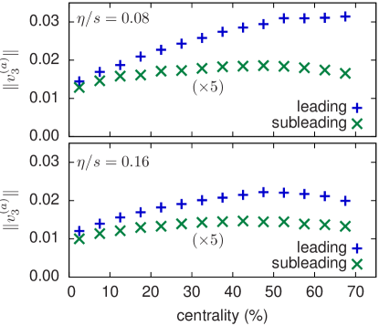
3.5 Average geometry in the subleading plane

In this section, we clarify the physical origin of the subleading flow by correlating the subleading hydrodynamic response with the geometry.

As a first step, we determined the average initial geometry in the principal component plane. Specifically, for each event the phase of the principal component $\xi^{(a)}_{n}$ [see Eq. (3.8)] defines orientation of the flow. We then rotate each event into $\xi^{(a)}_{n}$ plane and average the initial entropy density, $S({\bm{x}})\equiv\tau_{o}s(\tau_{o},{\bm{x}})$. More precisely, the event-by-event geometry in the principal component plane is defined to be

$$S(r,\phi;\,\xi^{(a)}_{n})\equiv\frac{1}{n}\sum_{\ell=0}^{n-1}S\left(r,\phi+(\arg\xi^{(a)}_{n}+2\pi\ell)/n\right)\,,$$ (3.18)

where we have averaged over the phases of $\sqrt[n]{\xi^{(a)}_{n}}$. Next, we average $S(r,\phi;\,\xi^{(a)}_{n})$ over all events weighted by the magnitude of the flow

$$\overline{S}(r,\phi;\,\xi^{(a)}_{n})\equiv\left<S(r,\phi;\,\xi^{(a)}_{n})|\xi^{(a)}_{n}|\right>.$$ (3.19)

Figure 3.5 shows the in-plane averaged geometry $\overline{S}(r,\phi;\,\xi^{(a)}_{3})$ for the leading and subleading principal components of the triangular flow in central collisions.

Figure 3.5: Average geometry$\times r^{3}$ in the leading and subleading principal component planes in central collisions minus an averaged radially symmetric background, $r^{3}(\overline{S}({\bm{x}};\,\xi^{(a)}_{3})-\left<S({\bm{x}})|\xi^{(a)}_{3}|\right>)$. Peak fluctuations are $\pm$10–20% above the background.

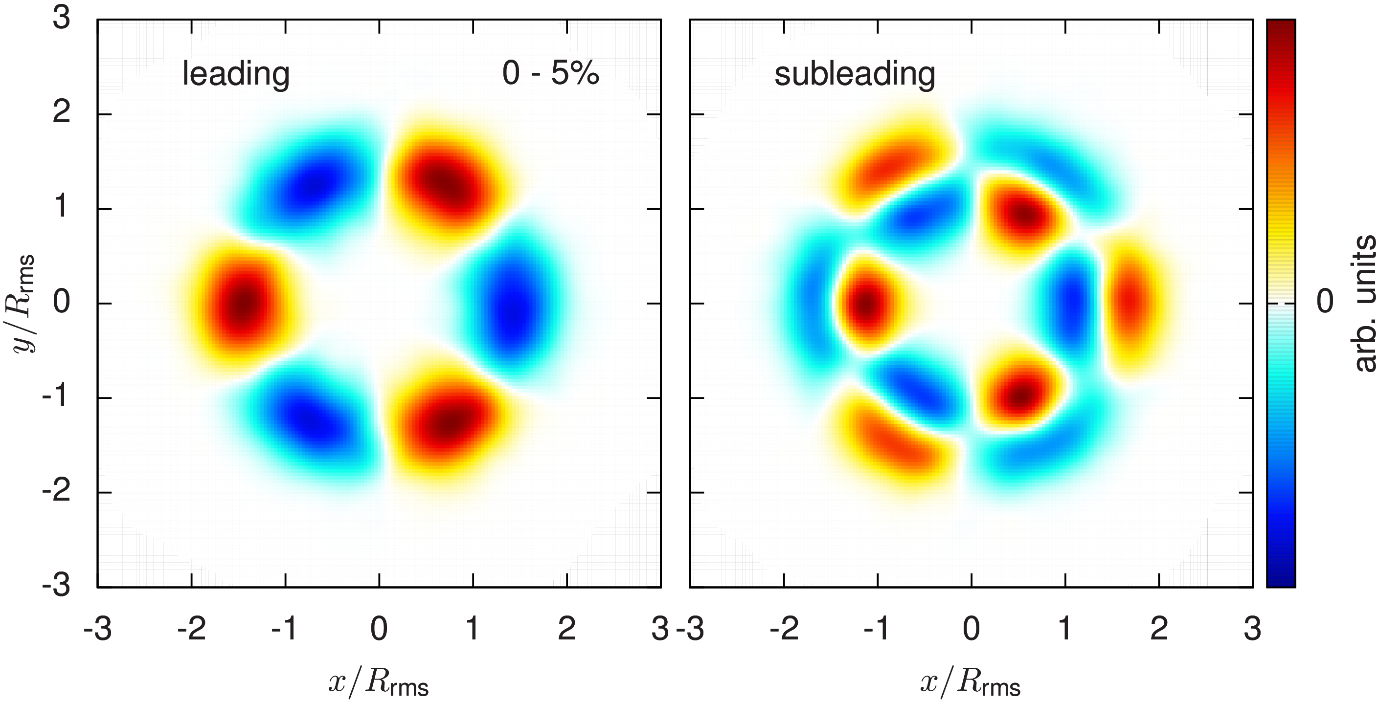
Clearly, the leading triangular principal component $V_{3}^{(1)}$ is strongly correlated with the triangular components of the initial geometry, while the subleading component $V_{3}^{(2)}$ is correlated with the radial excitations of this geometry. In central collisions, subleading flows of other harmonics $n=0\text{--}5$ are also predominantly correlated with radial excitations of the corresponding order eccentricity. However, in peripheral collisions, flow harmonics with significant nonlinear mixing, e.g. subleading $v_{2}$, $v_{4}$ and $v_{5}$, are not entirely due to radially excited geometry (as explained in Sec. 5.4) and thus the averaged geometry in the subleading principal component plane does not show sharp features of radial excitations.

To give a one-dimensional projection of Fig. 3.5, we integrate Eq. (3.19) over the azimuthal angle to define

$$\overline{S}_{n}(r;\,\xi^{(a)}_{n})\equiv\int_{0}^{2\pi}\!\!\!\text{d}\phi\,\overline{S}(r,\phi;\,\xi^{(a)}_{n})\,e^{in\phi}.$$ (3.20)

This is equivalent to defining $S_{n}(r)$,

$$S_{n}(r)\equiv\int_{0}^{2\pi}\!\!\!{d}\phi\,S(r,\phi)\,e^{in\phi}\,,$$ (3.21)

and correlating this with the flow fluctuation $\xi^{(a)}_{n}$

$$\overline{S}_{n}(r;\,\xi^{(a)}_{n})=\left\langle S_{n}(r)\xi^{*(a)}_{n}\right\rangle\,.$$ (3.22)

Results for the triangular geometry $\overline{S}_{3}(r;\,\xi^{(a)}_{3})r^{4}$ are shown by the blue (gray) curves in Fig. 3.6.

Figure 3.6: Correlation between the principal components and the triangular geometry, $\left\langle S_{3}(r)\xi^{*(a)}_{3}\right\rangle$, for the leading and subleading flows in central collisions. The result has been multiplied by $r^{4}$ and normalized by $\overline{S}_{\rm tot}R_{\rm rms}^{3}$, so that the area under the leading curve is approximately $\varepsilon_{3,3}^{\rm rms}$.

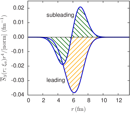
Again we see that the leading triangular flow originates from a geometric fluctuation with a large integrated eccentricity, while the subleading flow is sensitive to the radial excitation of the triangularity. We conclude that the relatively small subleading flow can correspond to a fairly significant fluctuation of the initial geometry.

3.6 Geometrical predictors

It is clear from Fig. 3.6 that usual geometric predictors based on a single coarse grained quantity like $\varepsilon_{n,n}$ cannot capture all the features of the radially excited geometry. In this section we will construct several geometric predictors for the leading and subleading flows following strategy outlined in Ref. [196]. Keeping the discussion general, let $\xi^{(a)}_{n\,\text{pred}}$ be a geometric quantity which predicts the event-by-event amplitude and phase of the corresponding flow $\xi^{(a)}_{n}$ . For example, for the leading $n=3$ component the triangularity $\varepsilon_{3,3}$ (defined below) is an excellent choice for $\xi_{3\,\text{pred}}^{(1)}$.

The geometric predictors are designed to maximize the correlation between a particular flow signal and the geometry. Specifically, the predictors maximize the Pearson correlation coefficient between the event-by-event magnitude and orientation of $a$th principal component, $\xi^{(a)}_{n}$, and the geometrical predictor $\xi^{(a)}_{n\,\text{pred}}$

$$\text{max}\quad Q^{(a)}_{n}=\frac{\big{<}\xi^{(a)}_{n}\xi^{*(a)}_{n\,\text{pred}}\big{>}}{\sqrt{\big{<}\xi^{(a)}_{n}{\xi^{*}_{n}}^{(a)}\big{>}\big{<}\xi^{(a)}_{n\,\text{pred}}\xi^{*(a)}_{n\,\text{pred}}\big{>}}}.$$ (3.23)

We constructed several predictors for the flow $\xi^{(a)}_{n}$ by assuming a linear relation between the flow and the geometry. The simplest predictor consists of linear combinations of the first two eccentricities of the initial geometry. These are defined as

$$\varepsilon_{n,n} \equiv-\frac{[r^{n}e^{in\phi}]}{R_{\rm rms}^{n}}\,,$$ (3.24a)

$$\varepsilon_{n,n+2} \equiv-\frac{[r^{n+2}e^{in\phi}]}{R_{\rm rms}^{n+2}}\,,$$ (3.24b)

where the square brackets $[\,]$ denote an integral over the initial entropy density for a specific event, normalized by the average total entropy $\bar{S}_{\text{tot}}$. $R_{\rm rms}\equiv\sqrt{\left\langle[r^{2}]\right\rangle}$ is the event averaged root-mean-square radius. Note that our definitions of $\varepsilon_{n,n}$ and $\varepsilon_{n,n+2}$ are chosen to make the event-by-event quantities $\varepsilon_{n,n}$ and $\varepsilon_{n,n+2}$ linear in the fluctuations. In this notation, the geometric predictor based on these eccentricities is

$$\xi_{n\,\text{pred}}^{(a)}=\varepsilon_{n,n}+c_{1}\,\varepsilon_{n,n+2},$$ (3.25)

where $c_{1}$ is adjusted to maximize the correlation coefficient in Eq. (3.23), and the overall normalization is irrelevant. While the first two eccentricities provide an excellent predictor for the leading flow, they do not predict the subleading flow very well. This is in part because the radial weight $r^{n+2}$ is too strong at large $r$.

More generally, one can define eccentricity as a functional of radial weight function $\rho(r)$:

$$\varepsilon_{n}\{\rho(r)\}\equiv-\frac{[\rho(r)e^{in\phi}]}{R_{\text{rms}}^{n}}.$$ (3.26)

It is the goal of this paper to find the optimal radial weight function $\rho(r)$ for predicting both leading and subleading flows.

It is evident from Fig. 3.6 that the leading and subleading geometries have different characteristic wave numbers. To find the optimal radial weight we expand $\rho(r)$ in radial Fourier modes

$$\rho(r)=\sum_{b=1}^{n_{k}}w_{b}\frac{2^{n}n!}{k_{b}^{n}}J_{n}(k_{b}r),$$ (3.27)

where $J_{n}(x)$ is a Bessel function of order $n$, $w_{b}$ are expansion coefficients, and $k_{b}$ are definite wavenumbers specified below. The prefactor is chosen so that for a single $k$ mode ($w_{1}=1,w_{b>1}=0$) at small $k$ ($kR_{\rm rms}\ll 1$) the generalized eccentricity approaches $\varepsilon_{n,n}$

$$\lim_{k\rightarrow 0}\varepsilon_{n}\{\rho(r)\}=\varepsilon_{n,n}.$$ (3.28)

At small $k$, we expand the $J_{n}(kr)$ and find

$$\varepsilon_{n}\{\rho(r)\}\simeq\varepsilon_{n,n}+c_{1}\,\varepsilon_{n,n+2},$$ (3.29)

where $c_{1}=-(kR_{\rm rms}/2)^{2}/(1+n)$. Thus the functional form of $\rho(r)$ adopted here yields a tunable linear combination of the eccentricities in Eq. (3.24), but the wave number parameter regulates the behavior at large $r$.

Figure 3.7: Quality plot (or Pearson correlation coefficient) for as a single $k$ mode predictor for principal triangular flows (central collisions).

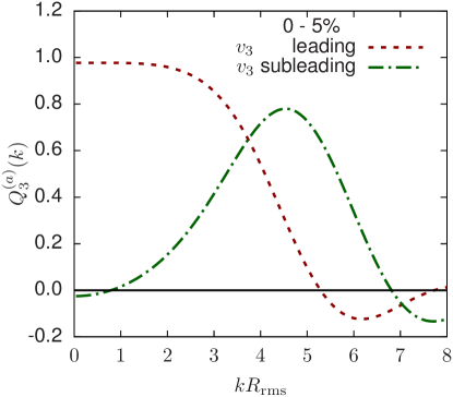
In Fig. 3.7 we show Pearson correlation coefficient $Q^{(a)}_{3}(k)$ between the triangular flow and a single $k$ mode predictor. We see that the leading triangular component is produced by low-$k$ fluctuations, while subleading flow originates from fluctuations at larger $k$. By using only two well chosen $k_{b}$ values for the Fourier expansion in Eq. (3.27) an approximately optimal radial weight can be found (see Fig. 3.8). Including additional $k$ modes in the functional form of $\rho(r)$ does not significantly improve the predictive power of the generalized geometric eccentricity. For the two $k$ modes we required (somewhat arbitrarily) that the ratio of $k$ values would be fixed to the ratio of the first two Bessel zeros:

$$\frac{k_{1}}{k_{2}}=\frac{j_{n,1}}{j_{n,2}}\,.$$ (3.30)

With this choice our basis functions were orthogonal in the interval $[0,R_{o}]$, where $k_{1}=j_{n,1}/R_{o}$. We then adjusted $R_{o}$ to maximize the correlation coefficient between $\varepsilon_{n}\{\rho(r)\}$ and the flow $\xi^{(a)}_{n}$. To account for changing system size with centrality, we used a fixed $R_{o}/R_{\text{rms}}$ ratio. In most cases we used $R_{o}/R_{\text{rms}}\approx 3.0$, but for all directed flow components ($\xi_{1}^{(1)}$ and $\xi_{1}^{(2)}$) and the second elliptic flow component ($\xi_{2}^{(2)}$), we found that $R_{o}/R_{\text{rms}}\approx 2.0$ optimized the correlation between the flow and the geometry.

Figure 3.8: Angle and magnitude correlations between the leading and subleading triangular flow and the optimal linear predictor based on two $k$ modes, Eq. (3.27).

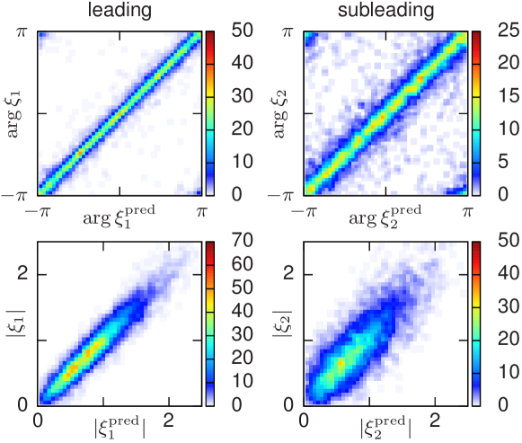
Ultimately, the assumption that the amplitude and phase of the flow is determined at least approximately by initial eccentricity, $\varepsilon_{n}\{\rho(r)\}$, is based on linear response. If nonlinear physics becomes important (as in the case of $v_{4}$ and $v_{5}$) then the predictors should be modified to incorporate this physics (see below and Ref. [196]). Thus, below we will refer to the $\varepsilon_{n}\{\rho(r)\}$ (with an optimized radial weight) as the best linear predictor and incorporate quadratic nonlinear corrections to the predictor as needed.

3.6.1 Testing linear response

The success of the linear flow predictors discussed in this work depends on the applicability of linear response. A straightforward way to check this assumption is to compare the averaged response of event-by-event hydrodynamics to the hydrodynamic response to suitably averaged initial conditions.

In Sec. 3.5 we computed the average geometry in the event planes of the leading and subleading triangular flows (see Fig. 3.5). It is straightforward to simulate this smooth initial condition and to compute the associated $V_{3}(p_{T})$. This is known as “single-shot” hydrodynamics in the literature [89]. In Fig. 3.9 we compare $V_{3}(p_{T})$ from the leading and subleading average geometries to the principal components $V_{3}^{(1)}(p_{T})$ and $V_{3}^{(2)}(p_{T})$ of event-by-event hydro.

Figure 3.9: Comparison of event-by-event hydro (averaged response) and single-shot hydrodynamics (response to average geometry) in central collisions. The singe-shot hydrodynamic results are generated from the initial conditions in Fig. 3.5.

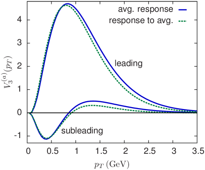
The qualitative features of both principal components are reproduced well by single-shot hydrodynamics, especially for the leading flow. It is particularly notable how the single-shot evolution reproduces the change of sign in $V_{3}^{(2)}(p_{T})$. However, in an important $p_{T}$ range, $p_{T}\sim 1.2\,{\rm GeV}$, the single-shot evolution misses the event-by-event curve for subleading flow by $\sim 30\%$.

It is useful to examine the time development of the subleading triangular flow in the single-shot hydrodynamics. In Fig. 3.10, we present three snapshots of the subleading flow evolution. The color contours show the radial momentum density per rapidity,

$$\tau T^{\tau r}=\tau(e+p)u^{\tau}u^{r}\,,$$ (3.31)

as a function of proper time $\tau$.

Figure 3.10: Hydrodynamic evolution of the subleading triangular flow for the averaged initial conditions shown in Fig. 3.5(b). The color contours indicate the radial momentum density per rapidity, $\tau T^{\tau r}$, while the arrows indicate the radial flow velocity.

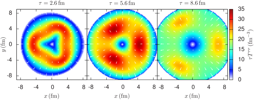
Shortly after the formation of the fireball, at $\tau=2.6\,{\rm fm}$ we observe negative triangular flow in Fig. 3.10(a). This flow is produced by the excess of material at small radii flowing into the “valleys” at larger radii [see Fig. 3.5(b)]. However, the radial flow has not developed yet, and therefore this phase of the evolution creates negative flow at small transverse momentum. After this stage, we see typical flow evolution of a triangular perturbation, i.e. the negative geometric eccentricity at small radii is transformed into positive triangular flow at large transverse momentum [see Figs. 3.10(b) and (c)]. The inner eccentricity dominates over the outer eccentricity at high $p_{T}$ because the radial flow has more time to develop before freeze-out, and because there is more material at small radii.

3.7 Results

In this section we report the principal component analysis summary and selected plots for flow harmonics $n=0\text{--}5$. The comprehensive list of figures for each harmonic is given in Appendix 3.A. Following the discussion of triangular flow in previous sections, we first identify the dominant principal components and then clarify their physical origin by finding an optimized geometric predictor as explained in Sec. 3.6. A new feature absent for the triangular flow is the nonlinear flow coupling to lower order principal components. We find that the subleading elliptic flow in peripheral collisions has a strong nonlinear coupling to the radial flow fluctuations $\xi_{0}^{(2)}$. We also find the nonlinear mixing in subleading $n=4$ and $n=5$ flow components.

3.7.1 Radial flow

Radial flow (or $V_{0}(p_{T})$) is the first term in the Fourier series, Eq. (3.3), and is by far the largest harmonic. Traditionally, the experimental and theoretical study of the fluctuations of $V_{0}(p_{T})$ (i.e., multiplicity and $p_{T}$ fluctuations) has been distinct from elliptic and triangular flow. There is no reason for this distinction.

Figure 3.11: (a) The $p_{T}$ dependence of the principal components of radial flow normalized by the average multiplicity, $v_{0}^{(a)}(p_{T})\equiv V_{0}^{(a)}(p_{T})/\left<dN/dp_{T}\right>$. (b) The Pearson correlation coefficient [Eq. (3.23)] between the subleading radial flow and various predictors versus centrality. The best linear predictor is described in Sec. 3.6.

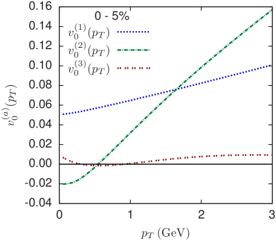
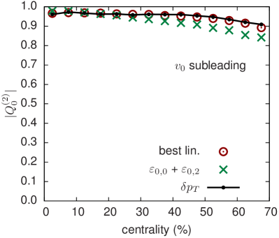
Examining the scaled $V_{0}(p_{T})$ eigenvalues shown in Fig. 3.11(a), we see that there are two large principal components. The first principal component is sourced by multiplicity fluctuations, i.e., the magnitude of $V_{0}(p_{T})$ fluctuates (but not its shape) due to the impact parameter variance in a given centrality bin. Corroborating this inference, Fig. 3.11(a) shows the momentum dependence of the leading principal component, which is approximately flat. Clearly this principal component is not particularly interesting, and the PCA procedure gives a practical method for isolating these trivial geometric fluctuations in the data set. The second principal component is of much greater interest, and shows a linear rise with $p_{T}$ that is indicative of the fluctuations in the radial flow velocity of the fluid [160].

In early insightful papers [201, 202], the fluctuations in the flow velocity (or mean $p_{T}$) were associated with the fluctuations in the initial fireball radius. These radial fluctuations are well described by both the eccentricities $(\varepsilon_{0,0}$, $\varepsilon_{0,2})$, Eq. (3.24), and the optimized eccentricity $\varepsilon_{0}\{\rho(r)\}$, Eq. (3.26). Therefore, as seen in Fig. 3.11(b), the subleading flow signal is strongly correlated with these linear geometric predictors.

Also shown in Fig. 3.11(b) is the correlation between subleading radial flow $\xi_{0}^{(2)}$ and mean transverse momentum fluctuations around the average

$$\delta p_{T}\equiv[p_{T}]-\left<[p_{T}]\right>.$$ (3.32)

Indeed, the subleading radial flow correlates very well with mean momentum fluctuations in all centrality bins.

In the next sections we will study the nonlinear mixing between the radial flow $\xi_{0}^{(2)}$ and all other harmonics.

3.7.2 Elliptic flow

Nonlinear mixing and elliptic flow

Figure 3.12: The magnitudes of the principal components of elliptic flow, $\|v^{(a)}_{2}\|$, versus centrality [see Eq. (3.10)].

Figure 3.13: The $p_{T}$ dependence of the principal components of elliptic flow normalized by the average multiplicity, $v_{2}^{(a)}(p_{T})\equiv V_{2}^{(a)}(p_{T})/\left<dN/dp_{T}\right>$, for central (0–5%) and peripheral collisions (45–50%).

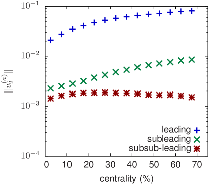
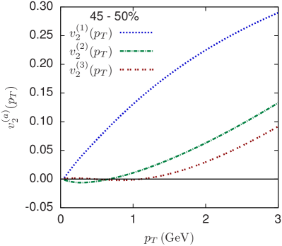
We next study the fluctuations of $V_{2}(p_{T})$ as function of centrality. As seen in Fig. 3.12, the principal component spectrum of elliptic flow in central collisions consists of two nearly degenerate subleading components in addition to the dominant leading component. This degeneracy is lifted in more peripheral bins. Comparing the $p_{T}$ dependence of the principal flows shown in Figs. 3.13(a) and 3.13(b), we see that going from central (0–5%) to peripheral (45–50%) collisions, the magnitude of the second principal component increases in size and its momentum dependence changes dramatically. By contrast, the growth of the third principal component is much more mild. This strongly suggests that the average elliptic geometry is more important for the subleading than the subsub-leading mode.

To find a geometrical predictor for the sub- and sub-sub-leading modes we first tried the best linear predictor $\varepsilon_{2}\{\rho(r)\}$. In Fig. 3.14(a) (the red circles), we see that the correlation coefficient between this optimal linear predictor and the subleading flow signal drops precipitously as a function of centrality. As we will explain now, this is because nonlinear mixing becomes important for the subleading mode.

The ellipticity of the almond shaped geometry in peripheral collisions is traditionally parametrized by eccentricity $\varepsilon_{2,2}$ and it serves as an excellent predictor for the leading elliptic flow. However, $\varepsilon_{2,2}$ does not completely fix the initial geometry, and the radial size of the fireball can fluctuate at fixed eccentricity. As explained in Sec. 3.7.1, the radial size fluctuations modulate the momentum spectrum of the produced particles, and for a background geometry with large constant eccentricity this generates fluctuations in the $p_{T}$ dependence of the elliptic flow, i.e., subleading elliptic flow. This subleading flow lies in the reaction plane following the average elliptic flow, but its sign (which is determined by $\delta p_{T}$) is uncorrelated with $\varepsilon_{2,2}$.

The orientation of the reaction plane in peripheral bins is strongly correlated with the integrated $v_{2}$ or the leading elliptic principal component $\xi_{2}^{(1)}$, while the mean $p_{T}$ fluctuations are tracked by the subleading radial flow component $\xi_{0}^{(2)}$. Therefore we correlated the sub- and sub-sub-leading elliptic flows with the product of the leading elliptic and radial flows, i.e. we computed the correlation coefficient in Eq. (3.23) with $\xi_{2,\rm pred}^{(2)}=\xi_{2}^{(1)}\xi_{0}^{(2)}$. Examining Fig. 3.14(a) (the black line), we see see that the correlation between the subleading elliptic flow and the nonlinear mixing rises with centrality, as the correlation with best linear predictor drops. Examining Fig. 3.14(b) on the other hand, we see that the subsub-leading elliptic flow has stronger correlation with the initial geometry than the nonlinear mixing. Combining best linear geometric predictor and quadratic mixing terms in the predictor, i.e.

$$\xi_{2\,\rm pred}^{(2)}=\varepsilon_{2}\{\rho(r)\}+c_{1}\xi_{2}^{(1)}\xi_{0}^{(2)},$$ (3.33)

we achieve consistently high correlations for all centralities [the blue diamonds in Fig. 3.14(a) and (b)].

Figure 3.14: Pearson correlation coefficient between the subleading elliptic flows and the best linear predictor [Eq. (3.26)] with and without the nonlinear mixing between the radial and leading elliptic flows, $\xi_{2}^{(1)}\xi_{0}^{(2)}$. (a) and (b) show the correlation coefficient for $v_{2}$ subleading and $v_{2}$ subsub-leading flows respectively.

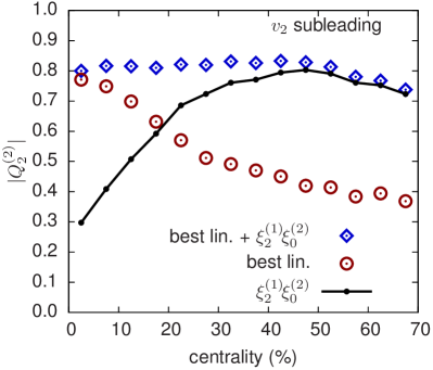
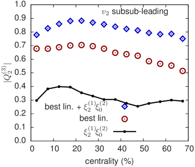
Dependence on viscosity

Figure 3.15: Pearson correlation coefficients for the subleading elliptic flow at viscosity over entropy ratio $\eta/s=0.16$. Dashed lines repeat $\eta/s=0.08$ results from Fig. 3.14(a) for the ease of comparison.

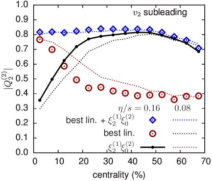
Before leaving this section we will briefly comment on the viscosity dependence of these results. Figure 3.15 shows a typical result for a slightly larger shear viscosity, $\eta/s=0.16$. As discussed above, the subleading elliptic flow [i.e., the event-by-event fluctuations in $V_{2}(p_{T})$] is a result of the linear response to the first radial excitation of the elliptic eccentricity, and a nonlinear mixing of radial flow fluctuations and the leading elliptic flow. In Fig. 3.15 we see that a slightly larger shear viscosity tends to preferentially damp the linear response leaving a stronger nonlinear signal. This is because the initial geometry driving the linear response has a significantly larger gradients due to the combined azimuthal and radial variations. Thus in Fig. 3.15 the linear response dominates the subleading flow only in very central collisions. These trends with centrality are qualitatively familiar from previous analyses of the effect of shear viscosity on the nonlinear mixing of harmonics [197, 203].

3.7.3 Triangular and directed flows

Figure 3.16: Pearson correlation coefficient between the subleading (a) directed and (b) triangular flows and the best linear predictor with and without radial flow mixing.

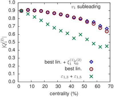
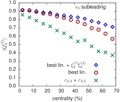
In Fig. 3.21(d) in the appendix we show the correlation coefficient between the leading flow amplitudes $\xi_{3}^{(1)}$ and the predicted amplitudes $\xi_{3}^{(1)\rm pred}$ using the optimal linear predictor and the $\varepsilon_{3,3}$, $\varepsilon_{3,5}$ fit. As is well known, the leading triangular mode is very well predicted by $\varepsilon_{3,3}$ and $\varepsilon_{3,5}$, though the quality degrades towards peripheral collisions [204]. As shown in Fig. 3.16(b), for the subleading flow the linear correlation coefficient is reduced relative to the leading flow, and a high degree of correlation is only achieved for the 0–40% centrality range. The simple geometric predictor based on $\varepsilon_{3,3}$ and $\varepsilon_{3,5}$ is reasonably correlated with the subleading flow in central collisions, but this correlation rapidly deteriorates in more peripheral collisions. The optimal linear predictor $\varepsilon_{3}\{\rho(r)\}$ based on two judiciously chosen $k$ values generally out performs all other predictors we studied for both leading and subleading flows. Adding the nonlinear mixing term $\xi_{0}^{(2)}\xi_{3}^{(1)}$ to the best linear predictor marginally improves the already good correlation with the subleading flow in peripheral collisions.

Directed flow exhibits many similarities to triangular flow. Specifically, the subleading directed flow is reasonably well correlated with the optimal linear predictor characterizing the radially excited dipolar geometry. Nonlinear mixing between the leading directed flow and the radial flow is unimportant [see Fig. 3.16(a)].

3.7.4 The $n=4$ and $n=5$ harmonic flows

Figure 3.17: Pearson correlation coefficient between the subleading $v_{4}$ and $v_{5}$ flows and the best linear predictor with and without several nonlinear terms [see Eqs. (3.37) and (3.38)].

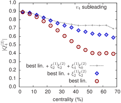
It is well known that the leading components of the $n=4$ and $n=5$ harmonics are determined by the nonlinear mixing of lower order harmonics in peripheral collisions [195, 89, 196, 197, 191].

For comparison with other works [196, 204], in the Appendix in Figs. 3.22(d) and 3.23(d) we construct a predictor based on a linear combination of the eccentricities

$$\varepsilon_{4,4}+c_{1}\varepsilon_{2,2}\varepsilon_{2,2}\quad\text{for }n=4,$$ (3.34)

$$\varepsilon_{5,5}+c_{1}\varepsilon_{2,2}\varepsilon_{3,3}\quad\text{for }n=5,$$ (3.35)

where here and below the coefficient $c_{1}$ is adjusted to maximize the correlation with the flow. This predictor is compared to a linear combination of the optimal eccentricity $\varepsilon_{n}\{\rho(r)\}$ and the corresponding nonlinear mixings of the leading principal components

$$\varepsilon_{4}\left\{\rho(r)\right\}+c_{1}\xi_{2}^{(1)}\xi_{2}^{(1)}\quad\text{for }n=4,$$ (3.36a)

$$\varepsilon_{5}\left\{\rho(r)\right\}+c_{1}\xi_{2}^{(1)}\xi_{3}^{(1)}\quad\text{for }n=5.$$ (3.36b)

Both sets of predictors perform reasonably well, though the second set has a somewhat stronger correlation with the flow.

Returning to the subleading components, we first correlated the best linear predictors, $\varepsilon_{4}\{\rho(r)\}$ and $\varepsilon_{5}\{\rho(r)\}$, with the corresponding subleading flow signals. As seen in Fig. 3.17 (the red circles), the correlation decreases rapidly with centrality, especially for $v_{4}$. Motivated by Eq. (3.36) which predicts the event-by-event leading $v_{4}$ and $v_{5}$ in terms $v_{2}$ and $v_{3}$, we construct a predictor for the subleading $v_{4}$ and $v_{5}$ in terms of the fluctuations of $v_{2}$ and $v_{3}$ (see Secs. 3.7.2 and 3.7.3, respectively). The full predictor reads

$$\varepsilon_{4}\left\{\rho(r)\right\}+c_{1}\xi_{2}^{(1)}\xi_{2}^{(2)}, \text{for }n=4,$$ (3.37a)

$$\varepsilon_{5}\left\{\rho(r)\right\}+c_{1}\xi_{2}^{(1)}\xi_{3}^{(2)}+c_{2}\xi_{3}^{(1)}\xi_{2}^{(2)}, \text{for }n=5.$$ (3.37b)

Including the mixings between the subleading $v_{2}$ and $v_{3}$ and the corresponding leading components greatly improves the correlation in mid-central bins (the blue diamonds). Finally, in an effort to improve the $v_{4}$ predictor in the most peripheral bins we have added additional nonlinear mixings between the radial flow and the leading principal components

$$\varepsilon_{4}\left\{\rho(r)\right\}+c_{1}\xi_{2}^{(1)}\xi_{2}^{(2)}+c_{2}\xi_{4}^{(1)}\xi_{0}^{(2)}, \text{for }n=4,$$ (3.38a)

$$\varepsilon_{5}\left\{\rho(r)\right\}+c_{1}\xi_{2}^{(1)}\xi_{3}^{(2)}+c_{2}\xi_{3}^{(1)}\xi_{2}^{(2)}+c_{3}\xi_{5}^{(1)}\xi_{0}^{(2)}, \text{for }n=5.$$ (3.38b)

As seen in Fig. 3.17(a) (the grey line) the coupling to the radial flow improves the correlation between the subleading $v_{4}$ and the predictor in peripheral collisions. On the other hand, for $v_{5}$, Fig. 3.17(b), all of the information about the coupling to the radial flow is already included in Eq. (3.37b) and adding $v_{0}$ does not improve the correlation.

3.8 Discussion

In this paper we classified the event-by-event fluctuations of the momentum dependent Fourier harmonics $V_{n}(p_{T})$ for $n=0\text{--}5$ by performing a principal component analysis of the two-particle correlation matrix in hydrodynamic simulations of heavy ion collisions. The leading principal component for each harmonic is very strongly correlated with the integrated flow, and therefore this component is essentially the familiar $v_{n}(p_{T})$ measured in the event plane. The subleading components describe additional $p_{T}$ dependent fluctuations of the magnitude and phase of $v_{n}(p_{T})$. The subleading flow is uncorrelated with the integrated $v_{n}$ and thus it is projected out in analyses of harmonic flow based on the scalar product or event plane methods. This paper focuses on the physical origins of the subleading flows, which are the largest source of factorization breaking in hydrodynamics.

First, we first studied the basic properties of principal components for the specific case of triangular flow such as its dependence on transverse momentum (Fig. 3.2), and centrality and shear viscosity (Fig. 3.4). The leading principle component of the triangular flow was found to be the hydrodynamic response to the participant triangularity, while the subleading flow (which is uncorrelated with the leading flow) is the hydrodynamic response to the first radial excitation of the triangularity. This conclusion was reached by averaging the event-by-event geometry in the event plane of the subleading flow (Fig. 3.5). The magnitude of this radial excitation is on par with the magnitude of the triangularity (Fig. 3.6), although the hydro response is smaller in magnitude. The triangular flow response is approximately linear to the geometrical deformation. This was checked by simulating the response to the average in-plane geometry with “single-shot” hydrodynamics (Fig. 3.10), and comparing this result to event-by-event hydrodynamics; i.e., we compared the response to the average with the averaged response (Fig. 3.9).

Having gained experience with triangular flow principal components, we conducted an extensive survey of principal flows for $n=0\text{--}5$ harmonics. We summarized the main results in Sec. 3.7, and for convenience reproduced PCA plots for all harmonics in the Appendix 3.A. Our systematic study started by placing radial flow (the $n=0$ harmonic) in the same framework as the other harmonic flows in Sec. 3.7.1. We identified the subleading $n=0$ principal component with mean $p_{T}$ fluctuations and confirmed (as is well known [201, 202]) that these fluctuations are predicted by the variance of the radial size of the fireball.

Next, we investigated the nature of the subleading elliptic flows in Sec. 3.7.2. The principal component analysis reveals that in central collisions there are two comparable sources of subleading elliptic flow, but they have strikingly different centrality dependence (see Figs. 3.12 and 3.13). In mid-peripheral collisions the first subleading component mainly reflects a nonlinear mixing between elliptic and radial flows, and this component is only weakly correlated with the radially excitations of the elliptic geometry. The second subleading component in this centrality range is substantially smaller and more closely reflects the radial excitations. In more central collisions, however, the nonlinear mixing with the average elliptic flow becomes small, and the sub and subsub-leading principal components become comparable in size. Thus, the rapid centrality dependence of factorization breaking in $v_{2}$ is the result of an interplay between the linear response to the fluctuating elliptic geometry, and the nonlinear mixing of the radial and average elliptic flows. Larger shear viscosity only strengthens the trend as shown in Fig. 3.15.

This nonlinear mixing can be confirmed experimentally by measuring the correlations between the principal components $\left\langle\xi_{2}^{(2)}(\xi_{2}^{(1)}\xi_{0}^{(2)})^{*}\right\rangle$ which is predicted in Fig. 3.14. The prediction is that three point correlation between the subleading elliptic event plane, the mean $p_{T}$ fluctuations, and the leading elliptic event plane defined by the $Q_{2}$ vector, i.e.,

$$\frac{\left\langle\xi_{2}^{(2)}\delta p_{T}Q_{2}^{*}\right\rangle}{\sqrt{\left\langle(\delta p_{T})^{2}\right\rangle\left\langle|Q_{2}|^{2}\right\rangle}},$$ (3.39)

changes rapidly from central to midperipheral collisions. This correlation is analogous to the three plane correlations such as $\left\langle V_{5}(V_{2}V_{3})^{*}\right\rangle$ measured previously [191].

In Sec. 3.7.3 the subleading directed and triangular flows were shown to be a linear response to the radial excitations of the corresponding eccentricity of the initial geometry. In these cases a generalized eccentricity $\varepsilon_{n}\{\rho(r)\}$ with an optimized radial weight (describing the radial excitation) provides a good predictor for the subleading flows (Fig. 3.16 and 3.8).

Finally, in Sec. 3.7.4 we studied factorization breaking in $v_{4}$ and $v_{5}$. With the comprehensive understanding of the fluctuations of $v_{2}$ and $v_{3}$ described above, the corresponding fluctuations in $v_{4}$ and $v_{5}$ were naturally explained as the nonlinear mixing of subleading $v_{2}$ and $v_{3}$ with their leading counterparts, together with linear response to the quadrangular and pentagonal geometries (see Fig. 3.17).

The study of the fluctuations in the harmonics spectrum presented here shows the power of the principal component method in elucidating the physics which drive the event-by-event flow. We hope that this motivates a comprehensive experimental program measuring the principal components and their correlations for $n=0-5$. Such an analysis would clarify the initial state in typical and ultra-central events with unprecedented precision, and would strongly constrain the dynamical response of the quark gluon plasma.

Appendices

Appendix 3.A List of figures

Here we present a comprehensive catalog of PCA plots for each harmonic $n=0\text{--}5$. Centrality dependence of flow magnitudes for $n=0$, appearing as Fig. 3.12 in the text above, is repeated here as Fig. 3.18(a), and analogous plots for other harmonics are given in Figs. 3.19(a)-3.23(a). The $p_{T}$ dependence of normalized principal components for radial and elliptic flows in central (0-5%) collisions shown in Figs. 3.11(a) and 3.13(a) are reproduced as Figs. 3.18(c) and 3.20(c) and complemented with Figs. 3.19(c) and 3.21(c)-3.23(c). Additionally, Figs. 3.18(b)-3.23(b) depict the same principal components, but without normalization by average multiplicity $\left<dN/dp_{T}\right>$. Finally, in the paper we showed the Pearson correlation coefficients for the subleading flows for each harmonic $n=0\text{-}5$ in Figs. 3.11(b),3.14(a),3.16(a), 3.16(b), 3.17(a) and 3.17(b), while in this appendix we show results for both leading and subleading flows in the series of figures Figs. 3.18(d)-3.23(d) and Figs. 3.18(e)-3.23(e).

(a)  Centrality dependence of the (scaled) magnitudes of flows $\|v^{(a)}_{0}\|$.

(b)  Momentum dependence of principal flow vectors $V_{0}^{(a)}(p_{T})$ in central collisions.

(c)  Principal flow vectors divided by the average multiplicity, $v_{0}^{(a)}(p_{T})\equiv V_{0}^{(a)}(p_{T})/\left<dN/dp_{T}\right>$.

(d)  Pearson correlation coefficient between the leading flow (zero suppressed for clarity) and several predictors.

(e)  Pearson correlation coefficient between the subleading flow and several predictors.

Figure 3.18: Principal component analysis for $n=0$ harmonic flow.

(a)  Centrality dependence of the (scaled) magnitudes of flows $\|v^{(a)}_{1}\|$.

(b)  Momentum dependence of principal flow vectors $V_{1}^{(a)}(p_{T})$ in central collisions.

(c)  Principal flow vectors divided by the average multiplicity, $v_{1}^{(a)}(p_{T})\equiv V_{1}^{(a)}(p_{T})/\left<dN/dp_{T}\right>$.

(d)  Pearson correlation coefficient between the leading flow (zero suppressed for clarity) and several predictors.

(e)  Pearson correlation coefficient between the subleading flow and several predictors.

Figure 3.19: Principal component analysis for $n=1$ harmonic flow.

(a)  Centrality dependence of the (scaled) magnitudes of flows $\|v^{(a)}_{2}\|$.

(b)  Momentum dependence of principal flow vectors $V_{2}^{(a)}(p_{T})$ in central collisions.

(c)  Principal flow vectors divided by the average multiplicity, $v_{2}^{(a)}(p_{T})\equiv V_{2}^{(a)}(p_{T})/\left<dN/dp_{T}\right>$.

(d)  Pearson correlation coefficient between the leading flow (zero suppressed for clarity) and several predictors.

(e)  Pearson correlation coefficient between the subleading flow and several predictors.

Figure 3.20: Principal component analysis for $n=2$ harmonic flow.

(a)  Centrality dependence of the (scaled) magnitudes of flows $\|v^{(a)}_{3}\|$.

(b)  Momentum dependence of principal flow vectors $V_{3}^{(a)}(p_{T})$ in central collisions.

(c)  Principal flow vectors divided by the average multiplicity, $v_{3}^{(a)}(p_{T})\equiv V_{3}^{(a)}(p_{T})/\left<dN/dp_{T}\right>$.

(d)  Pearson correlation coefficient between the leading flow (zero suppressed for clarity) and several predictors.

(e)  Pearson correlation coefficient between the subleading flow and several predictors.

Figure 3.21: Principal component analysis for $n=3$ harmonic flow.

(a)  Centrality dependence of the (scaled) magnitudes of flows $\|v^{(a)}_{4}\|$.

(b)  Momentum dependence of principal flow vectors $V_{4}^{(a)}(p_{T})$ in central collisions.

(c)  Principal flow vectors divided by the average multiplicity, $v_{4}^{(a)}(p_{T})\equiv V_{4}^{(a)}(p_{T})/\left<dN/dp_{T}\right>$.

(d)  Pearson correlation coefficient between the leading flow (zero suppressed for clarity) and several predictors.

(e)  Pearson correlation coefficient between the subleading flow and several predictors.

Figure 3.22: Principal component analysis for $n=4$ harmonic flow.

(a)  Centrality dependence of the (scaled) magnitudes of flows $\|v^{(a)}_{5}\|$.

(b)  Momentum dependence of principal flow vectors $V_{5}^{(a)}(p_{T})$ in central collisions.

(c)  Principal flow vectors divided by the average multiplicity, $v_{5}^{(a)}(p_{T})\equiv V_{5}^{(a)}(p_{T})/\left<dN/dp_{T}\right>$.

(d)  Pearson correlation coefficient between the leading flow (zero suppressed for clarity) and several predictors.

(e)  Pearson correlation coefficient between the subleading flow and several predictors.

Figure 3.23: Principal component analysis for $n=5$ harmonic flow.

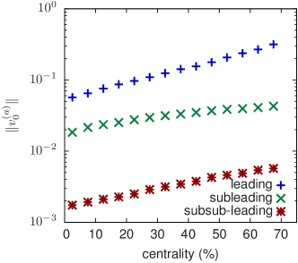
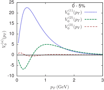
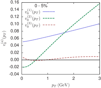
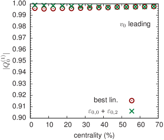
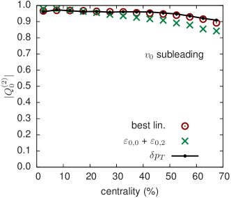
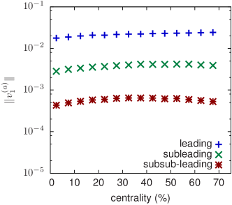
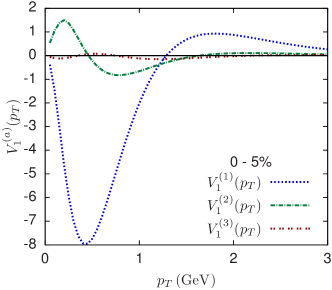
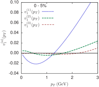
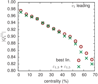
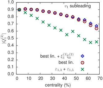
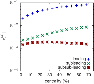
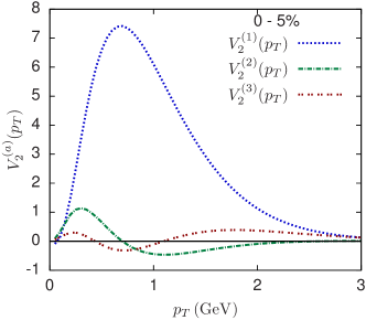
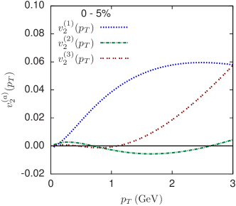
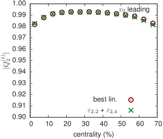
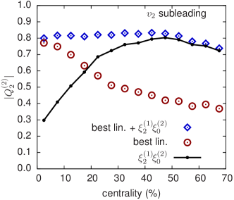
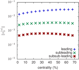
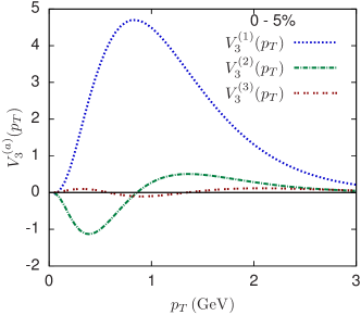
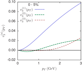
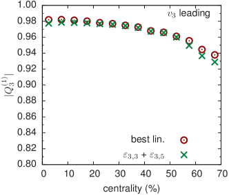
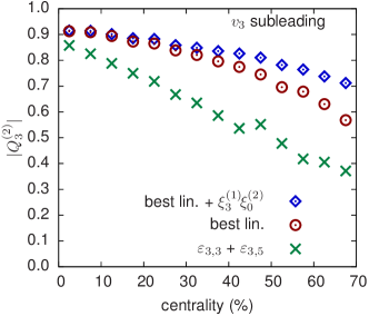
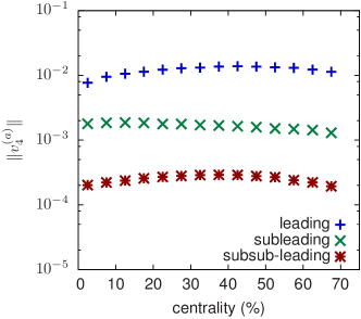
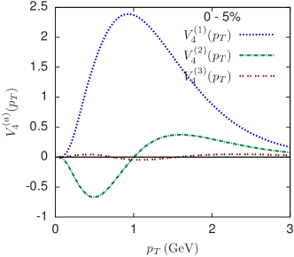
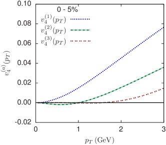
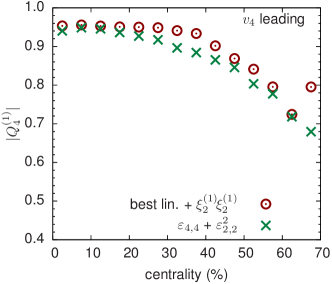
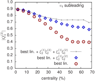
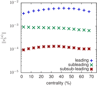
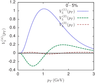
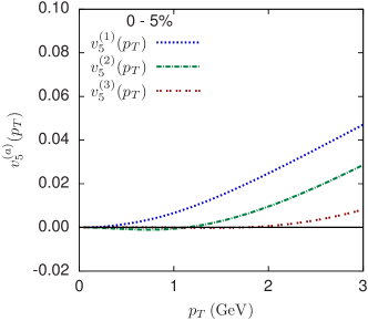
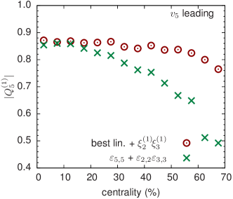
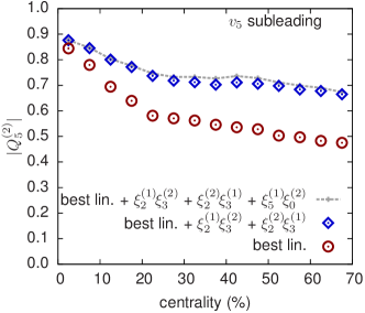
Chapter 4 Equilibration in weakly coupled effective kinetic theory

This chapter contains material published in

• L. Keegan, A. Kurkela, A. Mazeliauskas and D. Teaney, Initial conditions for hydrodynamics from weakly coupled pre-equilibrium evolution J. High Energ. Phys. 08, 171 (2016) [3]. Copyright (2016) by authors.

The discussion of the Green functions for the initial momentum perturbations, i.e. the Appendix C of the original publication, was omitted here.

4.1 Introduction

Viscous relativistic hydrodynamics provides a remarkably detailed and phenomenologically successful description of the expansion of the Quark Gluon Plasma (QGP) in the ultra-relativistic heavy-ion collisions realized at the BNL Relativistic Heavy Ion Collider (RHIC) and at the CERN Large Hadron Collider (LHC) [66, 67, 75]. Hydrodynamics is an effective theory based on an assumption that the medium is sufficiently close to local thermal equilibrium that the full stress tensor can be expanded in gradients of the energy and momentum densities [114]. However, due to the singular geometry of heavy ion collisions, the gradients diverge at early times, and the hydrodynamic approach does not apply during the initial stages of the evolution. Indeed, hydrodynamic simulations start at some sufficiently late initialization time $\tau_{\rm init}\sim 1\,\text{fm}/c$, when the gradient expansion becomes a useful approximation scheme. The initial conditions for hydrodynamics at $\tau_{\rm init}$ are generally unknown, and must be parametrized and fitted to data [205]. This procedure often neglects any prethermal evolution, and limits the empirical determination of the transport coefficients of the QGP [173].

A useful prethermal model should smoothly and automatically approach hydrodynamics. If this is the case, the combined pre-thermal and hydrodynamic evolutions will be independent of the initialization time [174, 175, 70]. In most simulations the prethermal evolution is either completely neglected [168], or modelled in a way that does not contain the correct physics to produce hydrodynamic flow [172, 171, 173]. In addition, in some models (such as the successful IP-glasma model [171] motivated by parton saturation) the initial conditions contain strong gradients which limit the effectiveness of the hydrodynamic derivative expansion [206, 207]. Different hydrodynamic codes regulate these extreme initial conditions in different ad hoc ways, e.g. by arbitrarily setting the shear stress tensor to zero when the hydrodynamics is initialized. Again, these ambiguities limit the ability of hydrodynamic simulations to determine the transport properties of the QGP.

In the limit of weak coupling $\alpha_{s}\ll 1$ the approach to hydrodynamics, or hydrodynamization, is described by an Effective Kinetic Theory (EKT) [140], which takes into account the non-trivial in-medium dynamics of screening and the Landau-Pomeranchuk-Migdal suppression of collinear radiation. In ref. [169] (which includes one of the authors), it was shown that the EKT, starting with initial conditions motivated by the Color-Glass Condensate (CGC) saturation framework [90, 91, 92, 93, 94], reaches hydrodynamics in a phenomenologically reasonable time scale of $\sim 10/Q_{s}$, where $Q_{s}$ is the (adjoint representation) saturation scale, which is estimated to be of order of few GeV for central heavy-ion collisions at the LHC. This first calculation used the EKT to monitor the equilibration of a uniform plasma of infinite transverse extent during a Bjorken expansion.

Transverse gradients in the profile will initiate flow during the equilibration process. This preflow and the accompanying modifications of the initial energy density profile will influence the subsequent hydrodynamic evolution. The goal of the current paper is to use the EKT to precisely determine the preflow and the components of the energy momentum tensor $T^{{\mu}\nu}(\tau_{\rm init},{\bf x}_{\perp})$ that should be used to initiate the hydrodynamic evolution for a given initial energy density profile. Although the kinetic theory calculation can be used to match different models for the initial energy profile to hydrodynamics, the weak coupling approximations made in the IP-glasma model lead naturally to effective kinetic theory.

Fig. 4.1 shows a typical transverse (entropy) profile that is used in

Figure 4.1: A typical entropy density profile (times ${\tau_{\rm init}}$) for a single event used as an initial condition in current hydrodynamic simulations at the LHC for a 0-5% centrality class [1]. An event averaged initial condition is shown by the dashed line. Often the initial flow velocity is set to zero. The different scales are discussed in the text.

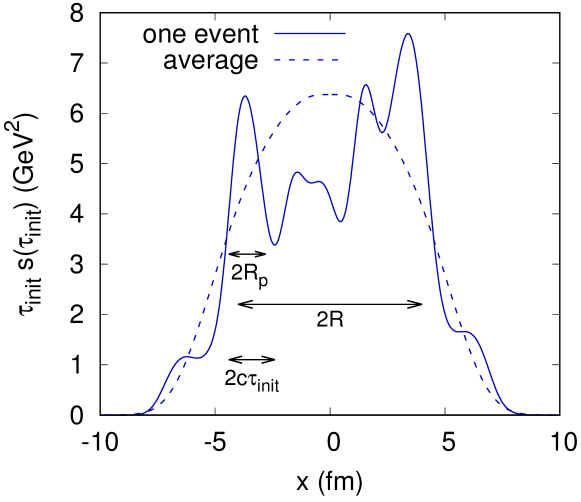
current hydrodynamic simulations [1]. Clearly during the equilibration process the profile will change and generate initial flow. The equilibration time, $c\tau_{\rm init}$, is short compared to the nuclear radius, $R$. For this reason the prethermal evolution is insensitive to the global collision geometry. Indeed, we may decompose the transverse plane into causally disconnected patches of size $c\tau_{\rm init}\ll R$ whose prethermal evolution can be separately determined. In these patches, the global nuclear geometry determines a small gradient that can be considered as a linear perturbation over a translationally invariant background. Thus, corrections to initial conditions for hydrodynamics from the global geometry are of order $c\tau_{\rm init}/R$ [208]. In addition to the global geometry, the initial energy density profile includes event-by-event fluctuations at smaller scales set by the nucleon size $R_{p}$, which is comparable to the causal horizon $R_{p}\sim c\tau_{\rm init}$. Event-by-event fluctuations at these length scales are suppressed by $1/\sqrt{N_{\text{part}}}$ where $N_{\text{part}}$ is the number of participating nucleons in the event, $N_{\text{part}}\sim 100-300$. Therefore, such fluctuations can also be treated in a linearized way as fluctuations over a translationally invariant background. The structure of the initial profile at even smaller scales is less well known, but in models based on CGC, one expects fluctuations to subnuclear scales of order the saturation momentum, $Q_{s}^{-1}\sim 0.1\,\text{fm}$.

Finally, an important scale is set by the mean free path, which in a weakly coupled theory is of order $1/\lambda^{2}T_{\rm eff}$ for states not too far from equilibrium. In practice, this length scale is comparable, though slightly shorter than the causal horizon and the nucleon scales. Without the scale separation, the medium prethermal response to initial perturbations in the transverse plane can only be computed by a calculation within the EKT. Fortunately, as discussed above linearized kinetic theory is sufficient to determine this response.

To summarize, our strategy is to use linearized kinetic theory to follow the hydrodynamization of energy perturbations on top of a far-from-equilibrium Bjorken background with translational symmetry in the transverse directions. This determines the stress tensor for hydrodynamics at the initialization time. The length scales of relevance are the nuclear-geometry, the nucleonic scale, the causal horizon $c\tau_{\rm init}$, and the mean free path

$$R\gg R_{p}\sim c\tau_{\rm init}\sim\frac{1}{\lambda^{2}T_{\rm eff}}\,.$$ (4.1)

By linearizing the problem and solving for the response, we will determine a Green function describing how an energy fluctuation at the earliest moments, $\tau\sim 1/Q_{s}$, evolves during the equilibration process to the hydrodynamic fields, i.e. the energy and momentum densities, $\delta T^{00}(\tau_{\rm init},{\bm{x}}_{\perp})$ and $\delta T^{0i}(\tau_{\rm init},{\bm{x}}_{\perp})$ respectively. We will verify that the subsequent evolution is described by second order hydrodynamics to certifiable precision.

In Sec. 4.2 we outline the linearized EKT, and study the linear response of the EKT in equilibrium. In Sec. 4.3 we systematically study the approach to equilibrium of Fourier modes of specified $k$, starting with a far from equilibrium initial state. In Sec. 4.4 we Fourier transform these results and determine a coordinate space Green function which produces the appropriate initial conditions for hydrodynamics at $\tau_{\rm init}$ when convolved with a specified initial state. We also analyze the long wavelength limit of these Green functions, making contact and providing additional insight into previous work on preflow [208]. Finally, we discuss our conclusions in Sec. 4.5.

4.2 Linearized kinetic theory

4.2.1 Setup

At weak coupling the non-equilibrium evolution of the boost invariant color and spin averaged gluon distribution function is described in terms of an effective kinetic equation [140]

$$\partial_{\tau}f_{{\bm{x}}_{\perp},{\bf p}}+\frac{\bf p}{|p|}\cdot\nabla_{{\bm{x}}_{\perp}}f_{{\bm{x}}_{\perp},{\bf p}}-\frac{p_{z}}{\tau}\partial_{p_{z}}f_{{\bm{x}}_{\perp},{\bf p}}=-\mathcal{C}[f_{{\bm{x}}_{\perp},{\bf p}}],$$ (4.2)

where the effective collision kernel $\mathcal{C}[f]$ incorporates the elastic $2\leftrightarrow 2$ and inelastic $1\leftrightarrow 2$ processes as required for a leading order description in the coupling constant $\lambda=4\pi\alpha_{s}N_{c}$, which is the only parameter of the EKT. The kinetic theory is valid when the occupancies are perturbative $\lambda f\ll 1$ and when the relevant distance scales are larger than the typical Compton wavelength of the particles $\Delta x\gtrsim\langle p\rangle^{-1}$. The details of the scattering kernel have been discussed in Refs. [140, 169, 170] and are briefly repeated here in the Appendix 4.A. We use the isotropic screening approximation from [169] which is leading order accurate for parametrically isotropic systems $\mathcal{P}_{L}/\mathcal{P}_{T}\approx 1$. (Here and below $\mathcal{P}_{L}$ and $\mathcal{P}_{T}$ denote the longitudinal and transverse pressures.) In the current paper we will consider only gluonic degrees of freedom and assume that the contribution of quarks is suppressed during the pre-equilibrium evolution.

We split the distribution function into a translationally symmetric background and a linearized perturbation with a wavenumber ${\bm{k}}_{\perp}$ in the transverse plane

$$f_{{\bm{x}}_{\perp},{\bf p}}=\bar{f}_{\bf p}+\int\frac{d^{2}{\bm{k}}_{\perp}}{(2\pi)^{2}}A({\bf k}_{\perp})e^{i{\bm{k}}_{\perp}\cdot{\bm{x}}_{\perp}}\delta f_{{\bm{k}}_{\perp},{\bf p}},$$ (4.3)

where $A({\bf k}_{\perp})$ characterizes the initial density profile. The kinetic equations for the background and the (complex) fluctuation then read

$$(\partial_{\tau}-\frac{p_{z}}{\tau}\partial_{p_{z}})\bar{f}_{{\bf p}} = -\mathcal{C}[\bar{f}],$$ (4.4a)

$$(\partial_{\tau}-\frac{p_{z}}{\tau}\partial_{p_{z}}+\frac{i{\bf p}_{\perp}\cdot{\bm{k}}_{\perp}}{p})\delta f_{{\bm{k}}_{\perp},{\bf p}} = -\mathcal{C}[\bar{f},\delta f],$$ (4.4b)

where $\mathcal{C}[\bar{f},\delta f]$ is the collision kernel linearized in $\delta f$ (see Appendix 4.A for details).

Figure 4.2: The dispersion relation of sound modes with thermal background from the EKT. The long wavelength modes are described by ideal hydrodynamics with $\omega=c_{s}k$ and $c_{s}^{2}=1/3$, and the approach to ideal hydrodynamics is well described by 2nd order hydrodynamics. For modes with wave numbers larger than $k\gtrsim 0.4T$, the dispersion relation differs significantly from the hydrodynamic expectation.

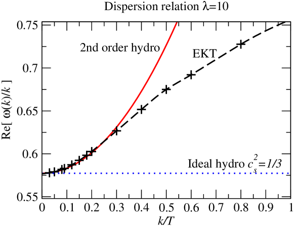
4.2.2 Hydrodynamization close to equilibrium

Before studying the equilibration process, we will analyze the linear response of the EKT close to equilibrium, corresponding to the $\tau\rightarrow\infty$ limit of (4.4). Our goal in this section is to determine at what wavenumbers (characterized by $k/T$) linearized energy-momentum perturbations are described by hydrodynamics for an equilibrated background.

The dispersion relation for the sound mode to second order in the hydrodynamic expansion reads [114]

$$\omega=c_{s}k-i\frac{4}{3}\frac{\eta}{e+p}k^{2}+\frac{4}{3}\frac{\eta}{e+p}\left(c_{s}\tau_{\pi}-\frac{2}{3c_{s}}\frac{\eta}{e+p}\right)k^{3},$$ (4.5)

where $c_{s}^{2}=1/3$ for conformal equation of state and $\eta,\tau_{\pi}$, are known transport coefficients at weak coupling [143, 209]. For $\lambda=10$ (corresponding to $\alpha_{s}\approx 0.26$) the hydrodynamic coefficients read $\eta/s=0.62$, $\tau_{\pi}=5.1\eta/sT$, and $\lambda_{1}=0.8\eta\tau_{\pi}$. We will quantify at what numerical values of $k/T$ the corrections to (4.5) become sizeable.

To this end, the kinetic theory is initiated in local thermal equilibrium with a spatially varying temperature, $T({\bm{x}})=T+\delta Te^{i{\bm{k}}_{\perp}\cdot{\bm{x}}_{\perp}}$, and corresponding phase space distribution

$$\delta f^{(1)}_{{\bm{k}}_{\perp},{\bf p}}=-\frac{\delta T}{T}p\,\partial_{p}\bar{f}_{{\bf p}},\quad\textrm{ and}\quad\bar{f}_{\bf p}=\frac{1}{e^{p/T}-1}.$$ (4.6)

Gradients in the energy density drive momentum perturbations in due course, and the frequency of the subsequent (damped) oscillations determines the real part of the dispersion relation. Numerically, we obtained the oscillation frequency by measuring the time interval between the successive nodes.

The results for various $k/T$ are depicted in Fig. 4.2 for $\lambda=10$. We see that at small $k$, $k/T\lesssim 0.1$, the dispersion relation is well described by the $c_{s}^{2}=1/3$ result of ideal hydrodynamics, and the approach to ideal hydrodynamics is described by the 2nd order corrections of (4.5) (note that the real part of the frequency does not get a first order correction). Indeed, for $k/T\lesssim 0.4$, the second order hydrodynamic theory matches well with the EKT.

At higher values of $k/T$, the EKT finally saturates at $\omega=k$ in contrast to the strict (unresummed) second order hydrodynamics. For $\lambda=10$ this happens only at rather large values of $k$, $k>T$. For these wavenumbers, the wavelength of the perturbation is comparable to the typical gluon Compton wavelength, and the linear response of the system cannot be reliably computed with kinetic theory in this regime.

We conclude that for $\lambda=10$, the smallest scales that hydrodynamize have $k\sim 0.4\,T$. Varying the value of $\lambda<10$ (not shown), we find that the scale where hydrodynamics breaks downs tracks the shear viscosity, $k\sim 0.4\,[\eta(\lambda=10)/\eta(\lambda)]\,T$ with varying $\lambda$. Note that for smaller $\lambda$, the saturation to $\omega\sim k$ can take place within the regime of validity of the effective theory.

4.3 Hydrodynamization of fluctuations far from equilibrium

We now move on to study the hydrodynamization of spatially dependent fluctuations on top of a far-from-equilibrium boost invariant background. As discussed in [210, 211, 212, 169], at very early times $\tau\lesssim Q_{s}^{-1}\,$ the far-from-equilibrium gluonic system in the midrapidity region is parametrically over-occupied $\lambda f\sim 1$, and the dynamics is described with coherent classical gauge fields rather than with particles. This part of the evolution is characterized by negative values of the longitudinal pressure $\mathcal{P}_{L}$, which is a result of the coherence of the approximately boost invariant fields. However, classical numerical simulations [94, 212] (as well as analytical series solutions to the classical equations of motion [213, 214]) show that in a timescale $Q_{s}\tau\sim 1$, the coherence is lost, the longitudinal pressure approaches zero $\mathcal{P}_{L}\sim 0$, and the occupancies become perturbative [215, 216, 99, 100]. At this point the system may be passed to the EKT [217, 218, 219, 169].

Following [169], we take as our initial condition at $\tau_{0}=1/Q_{s}$ a parametrization

$$f(p_{z},p_{\perp}) =\frac{2}{\lambda}Af_{0}(p_{z}\xi/p_{0},p_{\perp}/p_{0}),$$ (4.7)

$$f_{0}(\hat{p}_{z},\hat{p}_{\perp}) =\frac{1}{\sqrt{\hat{p}_{\perp}^{2}+\hat{p}_{z}^{2}}}e^{-2(\hat{p}_{\perp}^{2}+\hat{p}_{z}^{2})/3},$$ (4.8)

where $p_{0}=1.8\,Q_{s}$, $\xi=10$, and $\lambda=10$. The parameters $p_{0}$ and $\xi$ are motivated by classical simulations where $\sqrt{\left\langle p_{T}^{2}\right\rangle}\approx 1.8\,Q_{s}$ and $\left\langle p_{z}^{2}\right\rangle\ll\left\langle p_{T}^{2}\right\rangle$. The amplitude, $A$, is adjusted so that energy per rapidity

$$\tau_{0}e(\tau_{0})=\tau_{0}\nu_{g}\int\frac{d^{3}p}{(2\pi)^{3}}\,|p|\,f(p_{z},p_{\perp})\,,$$ (4.9)

matches the results of classical simulations [94], where

$$\tau_{0}e(\tau_{0})\simeq 0.358\,\frac{\tau_{0}\nu_{g}Q_{s}^{4}}{\lambda}\,.$$ (4.10)

Here $\nu_{g}=2d_{A}=16$ is the number of gluonic degrees of freedom. With these parameters, the number of gluons and the mean $p_{T}$ in the EKT at $\tau_{0}$ are

$$\frac{dN}{d^{2}{\bm{x}}_{\perp}dy}= 0.232\,\frac{\nu_{g}Q_{s}^{2}}{\lambda},\qquad\sqrt{\left\langle p_{T}^{2}\right\rangle}=1.8\,Q_{s},$$ (4.11)

which roughly matches the classical Yang-Mills simulations.

We will follow response to the specific initial perturbations of these initial conditions describing energy density fluctuations in the transverse plane

$$\delta f^{(1)}_{{\bm{k}}_{\perp},{\bf p}}(\tau_{0}) =-\frac{\delta Q_{s}}{Q_{s}}p\,\partial_{p}\bar{f}_{{\bf p}},$$ (4.12)

which results from varying the saturation scale in (4.7), $Q_{s}({\bm{x}}_{\perp})\sim Q_{s}+\delta Q_{s}e^{i{\bm{k}}_{\perp}\cdot{\bm{x}}_{\perp}}$.

Figure 4.3: (a) A comparison of the relevant combination $e(\tau)+T^{zz}(\tau)$ for the kinetic theory background with the hydrodynamic constitutive equations of (4.16a). (b) The background effective temperature as obtained from the Landau matching condition $e=\nu_{g}\frac{\pi^{2}}{30}T^{4}$. Extrapolation of first order hydro (fitted at asymptotic late times) is shown for comparison, Eq. (4.21). The scales in physical units correspond to $Q_{s}=1.4\,{\rm GeV}$ which yields the entropy required by hydrodynamic simulations (see text).

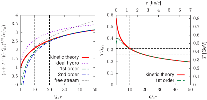
Without loss of generality, we can choose the wave vector $\hat{k}_{\perp}=(k,0)$ to point in $x$-direction. Then at any time, the energy and momentum perturbations are defined as

$$\delta e(\tau,k) \equiv\delta T^{00}=\nu_{g}\int\frac{d^{3}{\bf p}}{(2\pi)^{3}}p^{0}\delta f,$$ (4.13)

$$g^{x}(\tau,k) \equiv\delta T^{0x}=\nu_{g}\int\frac{d^{3}{\bf p}}{(2\pi)^{3}}p^{x}\delta f,$$ (4.14)

and their evolution is governed by the linearized conservation equations

$$\partial_{\tau}e(\tau)=-\frac{e(\tau)+T^{zz}(\tau)}{\tau},$$ (4.15a)

$$\partial_{\tau}\delta e(\tau,k)+ikg^{x}(\tau,k)=-\frac{\delta e(\tau,k)+\delta T^{zz}(\tau,k)}{\tau},$$ (4.15b)

$$\partial_{\tau}g^{x}(\tau,k)+ik\delta T^{xx}(\tau,k)=-\frac{g^{x}(\tau,k)}{\tau},$$ (4.15c)

where $\delta T^{\mu\nu}$ is the energy-momentum tensor perturbation caused by $\delta f$. If the system is described by hydrodynamics then $T^{zz}$, $\delta T^{zz}$ and $\delta T^{xx}$ are determined through the constitutive equations by the first moments of the particle distribution function $e$, $\delta e$ and $g^{x}$. For conformal second order viscous hydrodynamics these relations are

$$T^{zz}(\tau) =\frac{1}{3}e-\frac{4}{3}\frac{\eta}{\tau}-\frac{8}{9}\frac{\tau_{\pi}\eta-\lambda_{1}}{\tau^{2}},$$ (4.16a)

$$\delta T^{xx}(\tau,k)= \frac{\delta e(\tau,k)}{e}\left[\frac{1}{3}e+\frac{1}{3}\eta\tau_{\pi}k^{2}+\frac{1}{2\tau}\eta-\frac{2\left(\lambda_{1}-\eta\tau_{\pi}\right)}{9\tau^{2}}\right]$$

$$-i\frac{kg^{x}(\tau,k)}{e}\left[\eta-\frac{1}{\tau}\left(\frac{\eta^{2}}{2e}+\frac{\eta\tau_{\pi}}{2}-\frac{2}{3}\lambda_{1}\right)\right]$$ (4.16b)

$$\delta T^{zz}(\tau,k)= \frac{\delta e(\tau,k)}{e}\left[\frac{1}{3}e-\frac{1}{6}\eta\tau_{\pi}k^{2}-\frac{1}{\tau}\eta+\frac{4\left(\lambda_{1}-\eta\tau_{\pi}\right)}{9\tau^{2}}\right]$$

$$+i\frac{kg^{x}(\tau,k)}{e}\left[\frac{1}{2}\eta-\frac{1}{\tau}\left(\frac{\eta^{2}}{4e}+\frac{2}{3}\lambda_{1}\right)\right],$$ (4.16c)

where the constitutive equations for ideal (or first order viscous) hydrodynamics can be recovered by setting $\eta=\tau_{\pi}=\lambda_{1}=0$ (or $\tau_{\pi}=\lambda_{1}=0$).

4.3.1 Evolution of the background energy density

Before studying the perturbations, we will study the equilibration of the background energy density, elaborating on the original study [169]. In Fig. 4.3(a) we compare the energy momentum tensor combination $e+T^{zz}$ in the kinetic theory simulation to the constitutive equation, (4.16a). The $e+T^{zz}$ combination is motivated by the conservation law in (4.15a).

At early times the system evolves approximately according to free streaming, with $T^{zz}\sim 0$ and $e\propto\tau^{-1}$. As already noticed in [169], the constitutive equations give an increasingly accurate description of the EKT stress tensor as a function of time. While the ideal constitutive equations are rather far from the EKT at all relevant times, the viscous and 2nd order equations quickly converge to the EKT. Note that an accidental (approximate) cancellation of $\lambda_{1}-\eta\tau_{\pi}$ makes the second order correction anomalously small [199], and only at rather late times after non-hydrodynamic modes have almost completely decayed does second order hydrodynamics finally improve the first order result (not shown). By times $Q_{s}\tau=\{10,20\}$, the viscous constitutive equations agree with the EKT within $\{10\%,2\%\}$.

It is noteworthy that the EKT interpolates smoothly between the free streaming and viscous hydrodynamic evolutions without an extended period during which the evolution is not approximately described by one or the other approximation scheme. At $Q_{s}\tau{=}10$ the evolution is somewhat closer to free streaming, and using hydrodynamics at this point is a rough, though perhaps acceptable, approximation. At $Q_{s}\tau{=}20$ hydrodynamics is a better approximation, but at this time the causal horizon is becoming comparable to the nuclear radius.

Given the agreement with the constitutive equations, one can use the hydrodynamic equations to propagate the system forward in time. At late times ideal hydrodynamics is valid, and the entropy per area per rapidity approaches a constant

$$\lim_{\tau\rightarrow\infty}\tau s(\tau)\equiv\frac{\nu_{g}\Lambda_{s}^{2}}{\lambda}.$$ (4.17)

(Here the $\Lambda_{s}$ parametrization is motivated by the scaling of the initial multiplicity with the saturation scale in (4.10).) Dimensional reasoning indicates that $\Lambda_{s}^{2}$ is proportional to $Q_{s}^{2}$. Taking the data presented in Fig. 4.3(a) we may extrapolate $\tau\rightarrow\infty$ to determine the proportionality coefficient

$$\Lambda_{s}^{2}=1.95\,Q_{s}^{2}.$$ (4.18)

Here we have used the ideal equation of state to convert energy density to entropy density. Since the entropy per gluon of an ideal gluon gas is $3.6$, (4.18) implies the asymptotic number of gluons per area per rapidity is more than a factor of two larger than the input number of gluons at $\tau_{0}$

$$\left.\frac{dN}{d^{2}{\bm{x}}_{\perp}d\eta}\right|_{\tau\rightarrow\infty}=2.33\left.\frac{dN}{d^{2}{\bm{x}}_{\perp}d\eta}\right|_{\tau=\tau_{0}}.$$ (4.19)

At $Q_{s}\tau=\{10,20\}$ the entropy and gluon multiplicity have reached only {72, 82}% of their asymptotic values, corresponding to gluon multiplication factors of $\{1.6,1.9\}$ respectively.

Finally, let us make phenomenological contact with more complete hydrodynamic simulations of heavy ion collisions, and estimate the saturation momentum required by phenomenology. The initial entropy in hydrodynamics is normally adjusted to reproduce the mean multiplicity. Using the computer code from one such hydrodynamic simulation at the LHC [1], we computed the average entropy per area at the hydrodynamic initialization time

$$\left\langle\tau_{\rm init}s(\tau_{\rm init})\right\rangle=4.13\,{\rm GeV}^{2}.$$ (4.20)

Entropy production during the subsequent hydrodynamic evolution is small, approximately 15%, and therefore this constant is approximately independent of the initialization time. With Eqs. (4.17) and (4.18), setting $Q_{s}\simeq 1.4\,{\rm GeV}$ in the EKT will roughly reproduce the entropy in hydrodynamic simulations provided the system is passed to hydrodynamics at $Q_{s}\tau=10$ where the entropy in the EKT has reached 70% of its asymptotic value in (4.17).

In Fig. 4.3(b) we present the time evolution of the effective temperature (determined from the energy density and the equation of state) in physical units for $Q_{s}\simeq 1.4\,{\rm GeV}$. Its time dependence at late times is well described by first order viscous hydrodynamics with the asymptotic value

$$\lim_{\tau\rightarrow\infty}\left(T+\frac{2}{3}\frac{\eta}{s\tau}\right)\tau^{1/3}=0.763\,Q_{s}^{2/3}.$$ (4.21)

The temperature at $Q_{s}\tau{=}10$ is $T\simeq 430\,{\rm MeV}$, or close to three times the pseudo-critical temperature. At these temperatures, modern weakly coupled techniques can be expected to work reasonably, justifying our approximation scheme. Similarly, with this value of $Q_{s}$ an initialization time of $Q_{s}\tau\simeq 10$ corresponds to $\tau_{\rm init}\simeq 1.4\,{\rm fm}$. The elliptic and triangular flows in central events develop on a later time scale, of order $R/c_{s}\sim 8\,{\rm fm}$, and therefore an initialization time of this order may be acceptable. A more complete study including fermions will be needed to definitively answer this question.

4.3.2 Evolution of the perturbations

Figure 4.4: $\delta T^{xx}/T^{00}$ compared with hydrodynamic constitutive equations (the curves have been normalized by the magnitude of the initial perturbation $\delta T^{00}(\tau_{0})/T^{00}(\tau_{0})$). Long wavelengths with $k\lesssim 0.1\,T$ are described by the hydrodynamics at approximately the same time as the background $Q_{s}\tau\sim 10$. Shorter wavelengths with $k\sim 0.4\,Q_{s}$ are never well described by hydrodynamics.

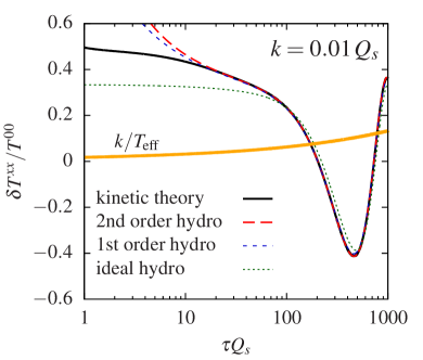
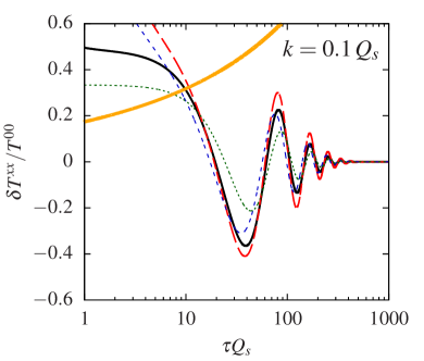
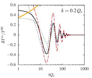
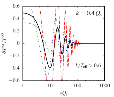
We now move on to describe the evolution of the linearized energy density perturbations on top of the thermalizing non-equilibrium background. We start with the initial condition of (4.12) with different values of $k/Q_{s}$. In figures 4.4(a)-(d) we show $xx$-component of perturbation energy momentum tensor $\delta T^{xx}$ compared with ideal, viscous, and second order hydrodynamic constitutive equations of Eq. (4.16b). The lines have been normalized by the background energy density $T^{00}(\tau)$, so that any observed damping is due to nontrivial dynamics associated to the spatial inhomogeneity.

We consider fixed values of $k/Q_{s}$, which do not correspond to fixed values of $k/T$, as the effective temperature is changing due to the expansion (see Fig. 4.4). For very large wavelengths with $k/Q_{s}=0.01$, we observe that while ideal constitutive equations have rather large corrections, these are well accounted for by the viscous and 2nd order equations, roughly at the same time as the background constitutive equation is satisfied, i.e. at times after $\tau\sim 10/Q_{s}$. Determining the temperature of the background from Landau matching condition $T^{4}=\nu_{g}\frac{\pi^{2}}{30}e$ (see Fig. 4.3 (right)), we find that at times $\tau=\{10,20\}/Q_{s}$, the wavelength $k=0.01Q_{s}$ in units of temperature $T=\{0.31,0.26\}Q_{s}$ is $k/T(\tau)=\{0.032,0.039\}$. As discussed in Sec. 4.2.2 and in Fig. 4.2 these values of $k/T$ are accurately described by second order hydrodynamics.

We see that even for larger $k/Q_{s}=\{0.1,0.2,0.4\}$ the hydrodynamic constitutive relations are approximately fulfilled when the background has hydrodynamized around $\tau\sim 10/Q_{s}$. However, larger values of $k/Q$ correspond to larger values of $k/T$, and even at late times there are corrections to the constitutive equations. While these corrections are moderate for $k/Q_{s}=0.2$ for which $k/T(\tau=10/Q_{s})\approx 0.6$, they remain $\mathcal{O}(1)$ for $k/Q_{s}=0.4$. It is therefore questionable whether it is justifiable to pass these short scales to hydrodynamic description at any time.

4.4 A Green function for hydrodynamics

We now move on to describe how the response to the linearized perturbations in EKT can be used in a hydrodynamic simulations to encapsulate the far-from-equilibrium dynamics of transverse perturbations during the time scales between $\tau\sim 1/Q_{s}$ and $\{10,20\}/Q_{s}$.

In order to construct the initial state for hydrodynamics at $\tau_{\rm init}$ from a given geometry at $\tau_{0}$, the linear response of the components of $T^{\mu\nu}$ to the initial perturbation are needed. The constitutive relations reduce the number of independent components of the energy momentum tensor, so it suffices to specify only $\delta T^{00}$ and $\delta T^{0x}$. Fig. 4.5(a) displays the energy and momentum response functions ($\tilde{E}(k;\tau,\tau_{0})$ and $\tilde{G}(k;\tau,\tau_{0})$ respectively) to an initial energy perturbation $\delta e(\tau_{0},k)$ in ${\bm{k}}$-space

$$\frac{\delta e(\tau,k)}{e(\tau)} \equiv\tilde{E}(k;\tau,\tau_{0})\frac{\delta e(\tau_{0},k)}{e(\tau_{0})},$$ (4.22)

$$\frac{g^{x}(\tau,k)}{e(\tau)} \equiv-i\tilde{G}(k;\tau,\tau_{0})\frac{\delta e(\tau_{0},k)}{e(\tau_{0})}.$$ (4.23)

The results are presented at two suggested initial times $\tau_{\rm init}=\{10,20\}/Q_{s}$. We will analyze the response functions at asymptotically small $k$ and in coordinate space in the next two subsections.

Figure 4.5: Normalized linear response functions in $k$-domain [Eqs. (4.22) and (4.23)] for the initial energy perturbation (a) at $Q_{s}\tau=10$ and (b) at $Q_{s}\tau=20$ .

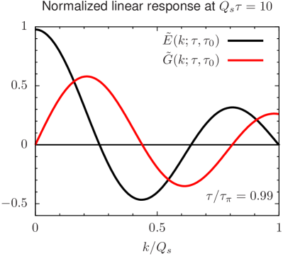
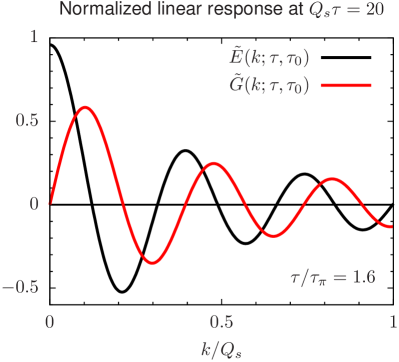
4.4.1 The kinetic theory response at asymptotically small $k$

The most important contribution to the flow arises from the average nuclear geometry, which is smooth on spatial scales of order $c\tau_{\rm init}$. For this reason the flow due to the average geometry is determined by the $k\rightarrow 0$ limit of the response functions. This section will provide an analytic understanding of this limit, i.e. the intercept of $\tilde{E}(k;\tau,\tau_{0})$ and the slope of $\tilde{G}(k;\tau,\tau_{0})$ in Fig. 4.5.

First, we will determine how the long wavelength energy perturbations in the transverse plane change as a function of time. Returning to the conservation equations, (4.15a) and (4.15b), and setting $k=0$, we have

$$\partial_{\tau}e(\tau)=-\frac{e(\tau)+T^{zz}(\tau)}{\tau},$$ (4.24)

$$\partial_{\tau}\delta e(\tau)=-\frac{\delta e(\tau)+\delta T^{zz}(\tau)}{\tau}.$$ (4.25)

From these equations the fractional perturbations in the transverse plane $\delta e/e$ remain constant in time in the free streaming limit (where $T^{zz}$ and $\delta T^{zz}$ are zero), and in the hydrodynamic limit (where $T^{zz}$ and $\delta T^{zz}$ are one third $e$ and $\delta e$). Outside of these limits $\delta e/e$ is not constant in time.

However, a constant of the motion at $k=0$ can be constructed whenever the hydrodynamic gradient expansion is applicable. Indeed, by dimensional analysis, an all order constitutive equation at $k=0$ must take the following form

$$T^{zz}=ef(e^{1/4}\tau),$$ (4.26)

where $f(x)$ is an order one function and $\delta T^{zz}=\partial_{e}T^{zz}\delta e$. Then straightforward steps show that to all orders in the gradient expansion

$$\lim_{k\rightarrow 0}\frac{\delta e(\tau,k)}{\,3e-T^{zz}}=\text{const.}$$ (4.27)

For conformally invariant theories with $T^{xx}{=}T^{yy}$ this can be written as

$$\lim_{k\rightarrow 0}\frac{\delta e(\tau,k)}{e+T^{xx}}=\text{const.}$$ (4.28)

In Fig. 4.6(a) we present the time evolution of $\delta e/e$ and $\delta e/(e+T^{xx})$ relative to their initial values. For our initial conditions $\delta e/(e+T^{xx})$ remains very nearly constant throughout the entire evolution. Using this result, the change in $\delta e/e$ can be determined by the ratio of $(e+T^{xx})/e$ at the initial and final times, when $T^{xx}$ is approximately $e/2$ and $e/3$ respectively. This reasoning leads to an asymptotic relation between the initial and final energy perturbations

$$\lim_{\tau\rightarrow\infty}\frac{\delta e(\tau)}{e(\tau)}=\frac{8}{9}\frac{\delta e(\tau_{0})}{e(\tau_{0})},$$ (4.29)

which is shown in Fig. 4.6(a).

Figure 4.6: (a) Normalized energy perturbation versus time in the (asymptotically) small $k$ limit. $8/9$ is the change in $(e+T^{xx})/e$ between free streaming and ideal hydrodynamic limits (see (4.29)). (b) The velocity perturbation versus time in the (asymptotically) small $k$ limit scaled by $-\partial^{x}e/(e+T^{xx})$ (see (4.34)). The result is compared to $\tfrac{1}{2}(\tau-\tau_{0})$ (see also ref. [208]) and first order hydrodynamics.

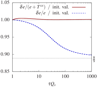
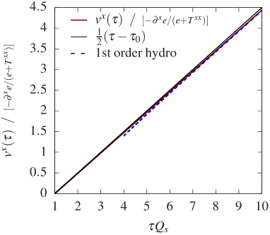
Next, we will determine the velocity at (asymptotically) small $k$ as a function of time from the pre-thermal evolution. From the conservation equations for perturbations, Eqs. (4.15b) and (4.15c), the momentum perturbations at small $k$ satisfy

$$\partial_{\tau}\left(\frac{\tau g^{x}}{ik}+\frac{1}{2}\delta e\tau^{2}\right)=-\frac{\tau}{2}\left(2\delta T^{xx}+\delta T^{zz}-\delta T^{00}\right).$$ (4.30)

For conformal theories with $\delta T^{xx}{=}\delta T^{yy}$ the right hand side of (4.30) is zero and

$$\frac{\tau g^{x}}{ik}+\frac{1}{2}\delta e\tau^{2}=\mbox{const}.$$ (4.31)

At late times and in coordinate space this condition reads

$$\frac{T^{0x}(\tau)}{T^{00}(\tau)}=-\frac{1}{2}\tau\frac{\partial_{x}T^{00}(\tau)}{T^{00}(\tau)}\,,$$ (4.32)

which was first noted in [208]. Here we have shown that this relation is a consequence of conformal symmetry (see also [208]) and the small $k$ limit.

Using (4.31) and the definition $g^{x}=(e+T^{xx})v^{x}$, the velocity as a function of time is given by

$$\frac{v^{x}}{ik}=-\frac{\tau}{2}\frac{\delta e}{e+T^{xx}}\,\left(1-\frac{\delta e(\tau_{0})\tau_{0}^{2}}{\delta e(\tau)\tau^{2}}\right).$$ (4.33)

Thus, after a brief transient period of order $\tau_{0}$, the velocity is directly proportional to time

$$v^{x}=\frac{\tau}{2}\,\left(\frac{-\partial^{x}e(\tau,{\bm{x}})}{e(\tau)+T^{xx}(\tau)}\right)\,,\qquad\frac{-\partial^{x}e(\tau,{\bm{x}})}{e(\tau)+T^{xx}(\tau)}={\rm const}.$$ (4.34)

In Fig. 4.6(b) we compare the growth of the velocity with time given by (4.33) with a simple estimate based on (4.34). The simple estimate does a remarkably good job for all times.

4.4.2 Response in coordinate space

To construct the initial conditions for hydrodynamics with the correct prethermal evolution, we determine the Green functions $E(|{\bm{x}}|;\tau,\tau_{0})$ and $G(|{\bm{x}}|;\tau,\tau_{0})$ which convert the initial profile of energy perturbations $\delta e(\tau_{0},{\bm{x}})$ to the required energy and momentum fluctuations at thermalization time

$$\frac{\delta e(\tau,{\bm{x}})}{e(\tau)} =\int d^{2}{\bm{x}}^{\prime}\frac{\delta e(\tau_{0},{\bm{x}}^{\prime})}{e(\tau_{0})}E(|{\bm{x}}-{\bm{x}}^{\prime}|;\tau,\tau_{0}),$$ (4.35a)

$$\frac{g^{i}(\tau,{\bm{x}})}{e(\tau)} =\int d^{2}{\bm{x}}^{\prime}\frac{\delta e(\tau_{0},{\bm{x}}^{\prime})}{e(\tau_{0})}\frac{({\bm{x}}-{\bm{x}}^{\prime})^{i}}{|{\bm{x}}-{\bm{x}}^{\prime}|}G(|{\bm{x}}-{\bm{x}}^{\prime}|;\tau,\tau_{0}).$$ (4.35b)

Currently hydrodynamic simulations often smooth the initial conditions before starting the hydrodynamic evolution by convolving the energy density with a Gaussian. In contrast, Eq. (4.35) smooths the initial conditions and generates pre-flow in a physical way, and provides an attractive alternative to this ad hoc procedure.

Figure 4.7: (top) Energy and (bottom) momentum Green functions, Eq. (4.35), for initial energy perturbation in coordinate space at (left) $Q_{s}\tau=10$ and (right) $Q_{s}\tau=20$.

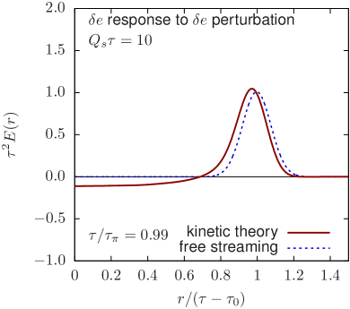
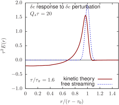
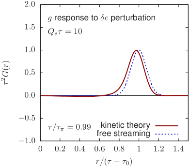
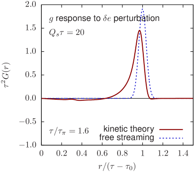
The EKT is applicable for distance scales that are larger than the Compton wavelength of the particles $\sim 1/Q_{s}$. This limits the accuracy of the Green function in spatial domain that can be reached in a computation based on kinetic theory. In order to fold this uncertainty into our result, we regulate our Green function by convoluting with a Gaussian weight, $e^{-r^{2}/2\sigma^{2}}/(2\pi\sigma^{2})$, with $r=|{\bm{x}}|$, and with a width of the order of the initial Compton wavelength $\sigma Q_{s}=0.7$. In momentum space this corresponds to suppressing the large $k$ contributions by an exponential envelope $\exp(-\sigma^{2}k^{2}/2)$

$$E(|{\bm{x}}|;\tau,\tau_{0}) =\int\frac{d^{2}{\bm{k}}}{(2\pi)^{2}}e^{i{\bm{k}}\cdot{\bm{x}}}e^{-\sigma^{2}k^{2}/2}E(|{\bm{k}}|;\tau,\tau_{0}),$$ (4.36)

$$G(|{\bm{x}}|;\tau,\tau_{0}) =\int\frac{d^{2}{\bm{k}}}{(2\pi)^{2}}(-i\hat{k}\cdot\hat{x})e^{i{\bm{k}}\cdot{\bm{x}}}e^{-\sigma^{2}k^{2}/2}G(|{\bm{k}}|;\tau,\tau_{0}).$$ (4.37)

The regulated Green functions are shown in Fig. 4.7 at the initialization times $\tau_{\rm init}Q_{s}=\{10,20\}$ (for details of the Fourier transform see Appendix 4.B.) At $\tau Q_{s}=10$ the system has spent a significant proportion of the total evolution time with small longitudinal pressure $T^{zz}\approx 0$, and therefore the resulting response is similar to the free streaming prediction (see Appendix 4.B). However, the Green function in Fig. 4.7(a) is peaked for $r{<}c|\tau-\tau_{0}|$, suggesting a slight deflection from the free streaming trajectory. Additionally, the energy perturbation is negative at small $r$, which is indicative of a nascent approach to hydrodynamics. At later times, such as $Q_{s}\tau=20$ in Fig. 4.7(b), these differences become more pronounced. Similar features are visible in the momentum response to an initial energy perturbation shown Fig. 4.7(c) and (d). Finally, in Fig. 4.8 we show the Green functions at later times $Q_{s}\tau=50$ and $Q_{s}\tau=500$, and compare to linearized second order hydrodynamics (Eqs. (4.15) and (4.16)) with initial conditions taken from the $Q_{s}\tau=\{10,20\}$ results. Between $Q_{s}\tau{=}20$ and $Q_{s}\tau{=}50$, the hydrodynamics overdamps the high $k$ modes (see also [220]), and the response is broader than the predictions of kinetic theory. However, these Green functions will be convolved with the initial conditions, and thus the resulting hydrodynamic initial state is mostly sensitive to the first moments of these kernels. The moments of the EKT and hydro kernels are determined by the small $k$ behaviour of the response functions, which agree to a few percent (not shown). At later times $Q_{s}\tau=500$, the response is largely determined by Fourier modes in the hydrodynamic regime $k\lesssim 0.1\,Q_{s}$, and the EKT and hydro kernels are visually similar.

To summarize, the hydrodynamic evolution sets in early at rather large anisotropies, and the hydrodynamic constitutive equations are approximately satisfied as soon as the $T^{zz}$ starts to significantly deviate from the free streaming expectation, $T^{zz}\approx 0$. For this reason the time interval when the evolution is not described by free streaming or hydrodynamics is comparatively brief (see Fig. 4.3(a)), and as hydrodynamics becomes marginally applicable at $Q_{s}\tau_{\rm init}\sim 10$, the Green function closely resembles the free streaming result. Therefore, an approach where the evolution is described by free streaming until $\tau_{\rm init}$ seems well motivated [172, 173], provided that the correct value of $\tau_{\rm init}$ is used. However, such an ad hoc approach does not account for some of the qualitative details of the Green function, such as the depletion of the energy density in the interior region.

Figure 4.8: Energy Green functions for initial energy perturbations in coordinate space at late times (a) $Q_{s}\tau=50$ and (b) $Q_{s}\tau=500$. The results are compared to linearized second order hydrodynamics (Eqs. (4.15) and (4.16)), with the initial conditions obtained from kinetic theory at $Q_{s}\tau{=}10$ and $Q_{s}\tau{=}20$ (see Fig. 4.5).

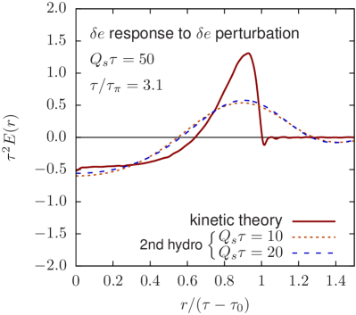
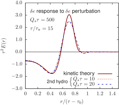
4.5 Discussion

In this paper, we have provided a bridge between the far-from-equilibrium initial conditions of heavy-ion collisions and hydrodynamized plasma. Our main result is the coordinate space Green functions (see Eq. (4.35) and Fig. 4.7), which can be used to filter the pre-equilibrium energy density to find the full energy-momentum tensor for hydrodynamics at the initialization time. The procedure can be implemented in complete hydrodynamic simulations, removing one source of uncertainty. Perhaps more importantly, the approximations in the EKT are compatible with the IP-Glasma setup, and thus the whole evolution from saturated nuclei to hydrodynamics can be comprehensively modelled within a perturbatively controlled framework.

We provide the coordinate space Green functions at two different suggested initialization times, $Q_{s}\tau_{\rm init}=\{10,20\}$. At the earlier initialization time, $Q_{s}\tau_{\rm init}=10$, there are significant (though bearable) corrections to the constitutive relations due to non-hydrodynamic modes (see Fig. 4.3(a) and Fig. 4.4). By $Q_{s}\tau_{\rm init}=20$ the constitutive relations at small $k$ are well satisfied, and the subsequent evolution is reasonably captured by second order hydrodynamics (see Fig. 4.8). The approximate overlap of the two 2nd order viscous lines in Fig. 4.8, which correspond to initializing the hydro at $\tau_{\rm init}Q_{s}=\{10,20\}$, demonstrates that the subsequent hydrodynamical evolution is indeed rather insensitive to the initialization time. In Sec. 4.4 we examined the (asymptotically) small $k$ limit of the Green functions, and confirmed (and clarified) a preflow estimate by Vredevoogd and Pratt [208] (see Fig. 4.6).

The hydrodynamics that the EKT follows is characterized by the weak coupling value of $\eta/s\approx 0.62$ [143], which is significantly higher than the AdS/CFT result $\eta/s\simeq 0.08$ [221], and current phenomenological estimates, which assume that $\eta/s$ is independent of the temperature. Recent analyses have relaxed the temperature independence of $\eta/s$, and shown that the value of $\eta/s$ at higher temperatures $T\sim 3T_{c}$ is poorly constrained by data [168]. Since it is the high temperature regime that is most relevant for the transition to hydrodynamics, we believe that the current kinetic theory results for the initial stages can be consistent with hydro phenomenology, provided $\eta/s$ decreases towards the strong coupling result as the system cools towards $T_{c}$.

Nevertheless, to apply our results to a hydro simulation with lower viscosity than the perturbative expectation, we note that the two initialization times $\tau_{\rm init}Q_{s}=\{10,20\}$ correspond in units of the hydro parameters to $\tau_{\rm init}=\{.99,1.6\}\tau_{\pi}$ or $T_{\text{init}}\tau_{\text{init}}/(4\pi\eta/s)=\{0.4,0.7\}$. The scaled times $\tau/\tau_{\pi}$ or $\tau T/(4\pi\eta/s)$ can be used to initialize simulations when the transport coefficients differ. Such an approach is supported by the reasonably good scaling properties of the hydrodynamization times and prethermal evolution as function of the coupling constant when expressed in terms of the hydrodynamic variables [169, 170].

Although our EKT description can be further improved by inclusion of fermionic degrees of freedom and by improving the connection to the early classical evolution, we believe that it already provides a physically sound picture of the approach to hydrodynamics and can be used to initialize all components of the energy-momentum tensor for subsequent hydrodynamic evolution. This eliminates a source of uncertainty in current simulations, and provides a satisfyingly complete description of the early time evolution in heavy ion collisions.

Microscopic initial state models like IP-Glasma also produce a non zero initial transverse flow at early times $\tau_{o}\sim 1/Q_{s}$, which should be propagated by EKT response functions analogous to Eq. (4.35). Then in linear response theory the energy and momentum flow at hydrodynamization time $\tau_{\text{init}}$ is a linear combination of contributions from initial energy and momentum perturbations. The demonstration of a smooth connection between initial conditions and hydrodynamics with kinetic theory pre-equilibrium in a realistic heavy ion simulation will appear in the follow up publication.

Appendices

Appendix 4.A Collision kernel

In this appendix we provide additional details on the collision kernels used in (4.4). The collision kernel for the uniform background contains terms arising from elastic $2\leftrightarrow 2$ scatterings and inelastic $1\leftrightarrow 2$ collinear splittings

$$\mathcal{C}[f]=\mathcal{C}_{2\leftrightarrow 2}[f]+\mathcal{C}_{1\leftrightarrow 2}[f].$$ (4.38)

The two collision terms read  [140, 169, 170]

$$\mathcal{C}_{2\leftrightarrow 2}[f]({\bf p}) =\frac{1}{4|{\bf p}|\nu_{g}}\int\frac{d^{3}k}{2k(2\pi)^{3}}\frac{d^{3}p^{\prime}}{2p^{\prime}(2\pi)^{3}}\frac{d^{3}k^{\prime}}{2k^{\prime}(2\pi)^{3}}|\mathcal{M}({\bf p},{\bm{k}};{\bf p}^{\prime},{\bm{k}}^{\prime})|^{2}(2\pi)^{4}\delta^{(4)}(P+K-P^{\prime}-K^{\prime})$$

$$\times\big{\{}f_{\bf p}f_{\bm{k}}[1+f_{{\bf p}^{\prime}}][1+f_{{\bm{k}}^{\prime}}]-f_{{\bf p}^{\prime}}f_{{\bm{k}}^{\prime}}[1+f_{{\bf p}}][1+f_{{\bm{k}}}]\big{\}}$$ (4.39)

and

$$\mathcal{C}^{1\leftrightarrow 2}[f]({\bf p}) =\frac{(2\pi)^{3}}{2|{\bf p}|^{2}\nu_{g}}\int_{0}^{\infty}dp^{\prime}dk^{\prime}\,\delta(|{\bf p}|-p^{\prime}-k^{\prime})\gamma({\bf p};p^{\prime}\hat{{\bf p}},k^{\prime}\hat{{\bf p}})\times\big{\{}f_{\bf p}[1+f_{p^{\prime}\hat{{\bf p}}}][1+f_{k^{\prime}\hat{{\bf p}}}]-f_{p^{\prime}\hat{{\bf p}}}f_{k^{\prime}\hat{{\bf p}}}[1+f_{{\bf p}}]\Big{\}}$$

$$+\frac{(2\pi)^{3}}{|{\bf p}|^{2}\nu_{g}}\int_{0}^{\infty}dp^{\prime}dk\,\delta(|{\bf p}|+k-p^{\prime})\gamma(p^{\prime}\hat{{\bf p}};{\bf p},k\hat{{\bf p}})\times\big{\{}f_{{\bf p}}f_{k\hat{{\bf p}}}[1+f_{p^{\prime}\hat{{\bf p}}}]-f_{p^{\prime}\hat{{\bf p}}}[1+f_{\bf p}][1+f_{k\hat{{\bf p}}}]\Big{\}},$$ (4.40)

where $\hat{{\bf p}}$ is the unit vector parallel to ${\bf p}$, and capital letters denote null 4-vectors, i.e. $P^{0}\equiv|{\bf p}|$. The effective elastic $|\mathcal{M}|^{2}$ and inelastic $\gamma$ scattering matrix elements contain non-trivial structures arising from the soft and collinear divergences, which are dynamically regulated by the in-medium physics.

For the most of kinematics the effective elastic scattering element is given by

$$|\mathcal{M}|^{2}=2\lambda^{2}\nu_{g}\left(9+\frac{(s-t)^{2}}{u^{2}}+\frac{(u-s)^{2}}{t^{2}}+\frac{(t-u)^{2}}{s^{2}}\right).$$ (4.41)

For a soft gluon exchange with the momentum transfer $q=|{\bf p}^{\prime}-{\bf p}|$ in $t$-channel (or $q=|{\bf p}^{\prime}-{\bm{k}}|$ in $u$-channel) the collision matrix is proportional to $\propto 1/(q^{2})^{2}$, and thus suffers from a soft Coulomb divergence. It is regulated by replacing

$$q^{2}t\rightarrow(q^{2}+2\xi_{0}^{2}m^{2})t,$$ (4.42)

in the denominators of divergent terms (similarly for the $u$-channel). Here $m^{2}$ is the thermal asymptotic mass of the gluon defined as

$$m^{2}=2\lambda\int\frac{d^{3}p}{(2\pi)^{3}}\frac{f_{\bf p}}{|{\bf p}|}.$$ (4.43)

The coefficient $\xi_{0}=e^{5/6}/\sqrt{8}$ is fixed so that the matrix element reproduces the drag and momentum diffusion properties of soft scattering at leading order for isotropic distributions $f_{{\bf p}}$ [219].

The effective splitting kernel reads

$$\gamma(p{\bf\hat{p}};p^{\prime}{\bf\hat{p}},k^{\prime}{\bf\hat{p}})=\frac{p^{4}+p^{\prime 4}+k^{\prime 4}}{p^{3}p^{\prime 3}k^{\prime 3}}\frac{\nu_{g}\lambda}{8(2\pi)^{4}}\int\frac{d^{2}h}{(2\pi)^{2}}2{\bf h}\cdot{\rm Re}{\bf F},$$ (4.44)

where the equation for ${\bf F}$ accounts for splitting due to multiple scatterings with transverse momentum exchange ${\bf}q$, and momentum non-collinearity

$$2{\bf h}= i\delta E({\bf h}){\bf F}({\bf h})+\frac{\lambda T_{*}}{2}\int\frac{d^{2}q_{\perp}}{(2\pi)^{2}}\mathcal{A}({\bf q}_{\perp})$$ (4.45)

$$\times\Big{[}3{\bf F({\bf h})}-{\bf F}({\bf h}-p^{\prime}{\bf q}_{\perp})-{\bf F}({\bf h}-k^{\prime}{\bf q}_{\perp})-{\bf F}({{\bf h}+p{\bf q}_{\perp}})\Big{]}.$$

with $T_{*}=\frac{\lambda}{m^{2}}\int\frac{d^{3}p}{(2\pi)^{3}}f_{\bf p}(1+f_{\bf p}),$ and $\delta E=m^{2}/2p^{\prime}+m^{2}/2k^{\prime}-m^{2}/2p+{\bf h}^{2}/2pk^{\prime}p^{\prime}$. In the isotropic screening approximation

$$\mathcal{A}({\bf q}_{\perp})=\left(\frac{1}{{\bf q}_{\perp}^{2}}-\frac{1}{{\bf q}_{\perp}^{2}+2m^{2}}\right).$$ (4.46)

Both $m^{2}$ and $T_{*}$ are self-consistently evaluated at each time step.

The linearized collision kernels are obtained trivially by replacing $f\rightarrow\bar{f}+\delta f$ in the integrands of 4.A and 4.A and linearizing in $\delta f$. In addition one has to take into account the linear variation of the thermal mass $\delta m^{2}$ and the effective temperature $\delta T_{*}$ in the scattering matrix elements Eqs. (4.41) and (4.44)

$$\delta m^{2} =2\lambda\int\frac{d^{3}p}{(2\pi)^{3}}\frac{\delta f_{\bf p}}{|{\bf p}|},$$ (4.47)

$$\delta T_{*} =\frac{\lambda}{m^{2}}\int\frac{d^{3}p}{(2\pi)^{3}}\delta f_{\bf p}(1+2f_{\bf p})-\frac{\delta m^{2}}{m^{2}}T_{*}.$$ (4.48)

where $m^{2}$ and $T_{*}$ are evaluated from the unperturbed background distribution.

Appendix 4.B Fourier transform of Green functions

Here we provide details of performing Fourier transforms in Eqs. (4.36) and (4.37) to obtain spatial Green functions shown in Figs. 4.7 and 4.8. The two dimensional Fourier transforms can be straightforwardly reduced to one dimensional Hankel transforms

$$E(|{\bm{x}}|;\tau,\tau_{0}) =\int_{0}^{\infty}\frac{dk}{2\pi}k\tilde{E}(k;\tau,\tau_{0})e^{-\sigma^{2}k^{2}/2}J_{0}(k|{\bm{x}}|),$$ (4.49)

$$G(|{\bm{x}}|;\tau,\tau_{0}) =\int_{0}^{\infty}\frac{dk}{2\pi}k\tilde{G}(k;\tau,\tau_{0})e^{-\sigma^{2}k^{2}/2}J_{1}(k|{\bm{x}}|).$$ (4.50)

Integrals in Eqs. (4.49) and (4.50) were done numerically by using cubic interpolation for $\tilde{E}$ and $\tilde{G}$ within the available range of wavenumbers $k\in[0,4]Q_{s}$ To avoid the oscillatory behaviour due to a sharp $k$ cut-off at $k=4Q_{s}$, we extrapolated the Green functions until the Gaussian envelope $e^{-\sigma^{2}k^{2}/2}$ smoothly cuts off the integral. For extrapolation at large $k$ we used functional forms motivated by free streaming results: $C_{0}J_{0}(v_{0}|k|(\tau-\tau_{0}))$ and $C_{1}J_{1}(v_{1}|k|(\tau-\tau_{0}))$, where coefficients $C_{i}$ and $v_{i}$ were fitted to match the oscillatory behaviour of Green functions at the largest available $k$. For $Q_{s}\tau=\{10,20,50\}$ we used $Q_{s}\sigma=0.7$ for the envelope corresponding roughly to the smallest scales the EKT can resolve. For $Q_{s}\tau=500$, perturbations with large wavenumbers were sufficiently suppressed by EKT evolution that no extrapolation was necessary.

For early times and large values of $k$ the collision terms in the Boltzmann equation (4.4) can be neglected and the system is freely streaming. For particle distributions that are highly anisotropic in $z$ direction ($\mathcal{P}_{L}\ll\mathcal{P}_{T}$), but isotropic in $xy$-plane, energy perturbations are propagating in circular wavefronts at the velocity $v$ of constituent particles (for massless gluons $v=c$). In such free streaming evolution energy perturbations at time $\tau$ and position ${\bm{x}}$ are equal to the average of energy perturbations at $\tau_{0}$ on a circle $|{\bm{x}}-{\bm{x}}^{\prime}|=c|\tau-\tau_{0}|$[173]. Thus, free streaming Green functions in coordinate space are

$$E(|{\bm{x}}|;\tau,\tau_{0})=G(|{\bm{x}}|;\tau,\tau_{0})=\frac{1}{2\pi|{\bm{x}}|}\delta(|\tau-\tau_{0}|-|{\bm{x}}|).$$ (4.51)

Free streaming Green functions shown in Fig. 4.7 were also folded in with a Gaussian regulator as discussed above.

Chapter 5 Non-linear noise corrections in Bjorken expansion

The following sections of this chapter are near verbatim reproduction of

• Y. Akamatsu, A. Mazeliauskas and D. Teaney, A kinetic regime of hydrodynamic fluctuations and long time tails for a Bjorken expansion Phys. Rev. C95, 014909 (2017) [4]. Copyright (2017) by the American Physical Society

5.1 Introduction

5.1.1 Overview

The purpose of the current paper is to develop a set of kinetic equations for hydrodynamic fluctuations, and to use these kinetic equations to study corrections to Bjorken flow arising from thermal fluctuations. The specific test case of Bjorken flow (which is a hydrodynamic model for the longitudinal expansion of a nucleus-nucleus collision [77]) is motivated by the experimental program of ultra-relativistic heavy-ion collisions at RHIC and the LHC. Detailed measurements of two particle correlation functions have provided overwhelming evidence that the evolution of the excited nuclear material is remarkably well described by the hydrodynamics of the Quark Gluon Plasma (QGP) with a small shear viscosity to entropy ratio of order $\eta/s\sim 2/4\pi$ [66, 67]. The typical relaxation times of the plasma, while short enough to support hydrodynamics, are not vastly smaller than the inverse expansion rates of the collision. For this reason the gradient expansion underlying the hydrodynamic formalism has been extended to include first and second order viscous corrections [114], and these corrections systematically improve the agreement between hydrodynamic simulations and measured two particle correlations [66]. Additional corrections, which have not been systematically included, arise from thermal fluctuations of the local energy and momentum densities and could be significant in nucleus-nucleus collision where only $\sim 20000$ particles are produced. This has prompted a keen practical interest in the heavy ion community in simulating relativistic hydrodynamics with stochastic noise [184, 185, 186, 187, 222, 189, 188]. In a non-relativistic context such simulations have reached a fairly mature state [223, 224, 225]. For a static fluid, thermal fluctuations give rise through the nonlinearities of the equations of motion to fractional powers in the fluid response function at small frequency, $G_{R}(\omega)\propto\omega^{3/2}$. Indeed, the “long-time tails” first observed in molecular-dynamics simulations [179, 180, 181] are a consequence of this non-analytic $\omega^{3/2}$ behavior. For Bjorken flow, the same nonlinear stochastic physics leads to fractional powers in the gradient expansion for the longitudinal pressure of the fluid. One of the goals of this manuscript is to compute the coefficient of the first fractional power in this expansion.

The measured two particle correlations in heavy ion collisions reflect both the fluctuations in the initial conditions and thermal fluctuations. Thermal fluctuations are believed to be a small (but conceptually important) correction to non-fluctuating hydrodynamics [185, 187, 186]. In addition, thermal fluctuations can become significant close to the QCD critical point [74, 222] and in smaller colliding systems such as proton-nucleus and proton-proton collisions [186], which show remarkable signs of collectivity [72].

In the current manuscript, rather than simulating nonlinear fluctuating hydrodynamics directly, we will reformulate fluctuating hydrodynamics as non-fluctuating hydrodynamics (describing a long wavelength background) coupled to a set of kinetic equations describing the phase space distribution of short wavelength hydrodynamic fluctuations. For Bjorken flow this set of equations can be solved to determine the first fractional powers in the gradient expansion.

5.1.2 Hydrodynamics with noise and fractional powers in the gradient expansion

At finite temperature, real-time dynamics in each regime of scales has an efficient and systematic description by an effective theory [226]. Hydrodynamics is a long wavelength effective theory which describes the evolution of conserved quantities by organizing corrections in powers of gradients. For the hydrodynamic expansion to apply we require frequencies under consideration to be small compared to the microscopic relaxation rates

$$\epsilon\equiv\frac{\omega\eta}{(e+p)c_{s}^{2}}\ll 1\,,$$ (5.1)

where we have estimated the microscopic relaxation time with the hydrodynamic parameters, $\tau_{R}\equiv\eta/(e+p)c_{s}^{2}$ [75] and for later convenience defined $\epsilon\equiv\omega\tau_{R}$.

For definiteness, we follow precedent [227, 114, 182] and consider a conformal neutral fluid driven from equilibrium by a small metric perturbation $h_{xy}(\omega)$ of frequency $\omega$. Within the framework of linear response (see Sec. 5.2 and Ref. [228] for further details), the stress tensor at low frequency takes the form

$$\delta T^{xy}=-h_{xy}(\omega)\Big{(}p-i\omega\eta+\left(\eta\tau_{\pi}-\frac{\kappa}{2}\right)\omega^{2}\Big{)}.$$ (5.2)

The first term is the prediction of ideal hydrodynamics $\delta T^{xy}=-ph_{xy}$; the middle term is the prediction of first order viscous hydrodynamics [227], where $\eta$ is the shear viscosity; finally, the last term is the prediction of second order hydrodynamics, where $\tau_{\pi}$ and $\kappa$ are the associated second order parameters [114].

In writing Eq. (5.2) we have neglected additional contributions stemming from fluctuations which will be described below. Thermal fluctuations can be incorporated into the hydrodynamic description by including stochastic terms into the equations of motion [177, 178][for a recent review: 104]

$$d_{\mu}T^{\mu\nu}=0,\quad T^{\mu\nu}=T^{\mu\nu}_{\text{ideal}}+T^{\mu\nu}_{\text{visc.}}+S^{\mu\nu},$$ (5.3)

where variance of the noise, $\left\langle S^{\mu\nu}S^{\rho\sigma}\right\rangle{\sim}2T\eta\delta(t-t^{\prime})$, is determined by the fluctuation dissipation theorem at temperature $T$ and introduces no new parameters into the effective theory. After including these stochastic terms, the correlators of momentum and energy evolve to their equilibrium values in the absence of the external force, $h_{xy}(\omega)$. Specifically, the equilibrium two point functions of the energy and momentum densities, $\delta e(t,{\bm{x}})\equiv T^{00}(t,{\bm{x}})-\left\langle T^{00}\right\rangle$ and $g^{i}(t,{\bm{x}})\equiv T^{0i}$ respectively, approach the textbook result [177]

$$\left\langle\delta e(t,{\bm{k}})\delta e(t,-{\bm{k}}^{\prime})\right\rangle =\frac{(e+p)T}{c_{s}^{2}}\;(2\pi)^{3}\delta^{3}({\bm{k}}-{\bm{k}}^{\prime}),$$ (5.4a)

$$\left\langle g^{i}(t,{\bm{k}})g^{j}(t,-{\bm{k}}^{\prime}))\right\rangle =(e+p)T\;\delta^{ij}(2\pi)^{3}\delta^{3}({\bm{k}}-{\bm{k}}^{\prime}),$$ (5.4b)

where $c_{s}$ is the speed of sound, and $\delta e(t,{\bm{k}})$ notates the spatial Fourier transform of $\delta e(t,{\bm{x}})$. In the presence of an external force or a non-trivial expansion these correlations are driven away from equilibrium. The purpose of hydrodynamics with noise is to describe in detail these deviations from equilibrium.

Due to the nonlinear character of hydrodynamics the thermal fluctuations change the evolution of the system. Indeed, a diagrammatic analysis of the hydrodynamic response at one-loop order shows that the stress in the presence of a weak external field (or the retarded Green function) is

$${\left\langle T^{xy}(\omega)\right\rangle}=-h_{xy}(\omega)\left(p-i\omega\eta+(i+1)\frac{\left(7+\left(\tfrac{3}{2}\right)^{3/2}\right)}{240\pi}T\left(\frac{\omega}{\gamma_{\eta}}\right)^{3/2}+\mathcal{O}(\omega^{2})\right),$$ (5.5)

where $p$, $e$, and $\eta$ are renormalized physical quantities (see Sec. 5.2.1 and Sec. 5.2.2 for further discussion of the renormalization), and

$$\gamma_{\eta}\equiv\frac{\eta}{e+p}\,,$$ (5.6)

is the momentum diffusion coefficient  [183, 182]. As emphasized and estimated previously, the fractional order $\omega^{3/2}$ is parametrically larger than second order hydrodynamics [182]. However, the coefficient of the $\omega^{3/2}$ terms is vanishingly small in weakly coupled theories and in strongly coupled theories at large $N_{c}$, and therefore second order hydrodynamics may be an effective approximation scheme except at very small frequencies. In the context of holography, the $\omega^{3/2}$ term can only be determined by performing a one loop calculation in the bulk [229].

In the current paper we will rederive Eq. (5.5) using a kinetic description of short wavelength hydrodynamic fluctuations. For an external driving frequency of order $\omega$, we identify an important length scale set by equating the damping rate and the external frequency

$$\gamma_{\eta}k_{*}^{2}\sim\omega\,,\quad k_{*}\sim\left(\frac{\omega}{\gamma_{\eta}}\right)^{1/2}\,.$$ (5.7)

We will refer to the $k_{*}$ as the dissipative scale below (see also Ref. [229]). Modes with wavenumbers significantly larger than the dissipative scale, $k\gg k_{*}$, are damped and reexcited by the noise on a time scale which is short compared to period $2\pi/\omega$, and this rapid competition leads to the equilibration of these shorter wavelengths, i.e. their equal time correlation functions are given by Eq. (5.4). By contrast, modes with wavenumbers of order $k\sim k_{*}$ have equal time correlation functions which deviate from the equilibrium expectation values.

Figure 5.1: The hydro-kinetic description of noise is based on the separation of scales between the long wavelength hydrodynamic background (with $k\sim\omega/c_{s}$), and shorter wavelength hydrodynamic fluctuations (with $k\sim k_{*}\equiv\sqrt{\omega/\gamma_{\eta}}$). The wavelengths of the hydrodynamic fluctuations are still much longer than microscopic mean free path. The hydrodynamic fluctuations are driven out of equilibrium by the expanding background, and this deviation is the origin of the long-time tail correction to the stress tensor.

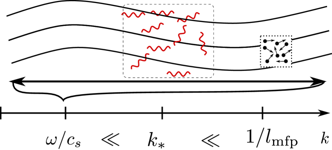
It is notable that the wavenumbers of interest $k_{*}$ are large compared to $\omega/c_{s}$, but still small compared to microscopic wavenumbers of order the inverse mean free path . Estimating the mean free path as $\ell_{\rm mfp}=c_{s}\tau_{R}$, we see that the strong inequalities

$$\frac{\omega}{c_{s}}\ll k_{*}\ll\frac{1}{\ell_{\rm mfp}},$$ (5.8)

can be written as

$$\frac{\omega}{c_{s}}\ll\frac{\omega}{c_{s}}\,\frac{1}{\sqrt{\epsilon}}\ll\frac{\omega}{c_{s}}\,\frac{1}{\epsilon},$$ (5.9)

and thus holds whenever hydrodynamics is applicable, $\epsilon\ll 1$. The scale separation illustrated in Fig. 5.1 can be used to set up an approximation scheme where modes of order $k_{*}$ on a soft ($k\sim\omega/c_{s}$) background are treated with a kinetic or Wentzel-Kramers-Brillouin (WKB) type approximation scheme. We will develop the appropriate kinetic equations in Sec. 5.2. These kinetic equations can be solved and used to determine how the two point functions of energy and momentum with wavenumbers of order $k_{*}$ deviate from equilibrium when driven by an external perturbation. The $\omega^{3/2}$ term in Eq. (5.5) roughly represents the contribution of $\int k^{2}dk{\sim}k_{*}^{3}$ slightly out of equilibrium hydro-kinetic modes per volume, with each mode contributing $\tfrac{1}{2}T$ of energy to the stress tensor. Note that the contribution to the stress tensor of modes outside of the kinetic regime $k\ll k_{*}$ is suppressed by phase space.

Similar kinetic equations can be derived for much more general flows. We will establish the appropriate kinetic equations for a Bjorken expansion [77], which is a useful model for the early stages of a heavy ion collision. The ideal, first, and second order terms in the gradient expansions have been given in Refs. [77],  [53],  and [114, 115] respectively. For a conformal (non-fluctuating) fluid the longitudinal pressure during a Bjorken expansion takes the form

$$\tau^{2}T^{\eta\eta}=p-\frac{4}{3}\frac{\eta}{\tau}+\frac{8}{9\tau^{2}}(\lambda_{1}-\eta\tau_{\pi})+\ldots\,.$$ (5.10)

The expansion rate is $\partial_{\mu}u^{\mu}=1/\tau$, and each higher term in the gradient expansion is suppressed by an integer power of $1/\tau T$. For Bjorken flow the expansion rate plays the role of frequency, and the distribution of sound modes are characterized by a dissipative scale analogous to Eq. (5.7) of order

$$k_{*}\sim\frac{1}{(\gamma_{\eta}\tau)^{1/2}}.$$ (5.11)

At this scale the viscous damping rate balances the expansion rate. These hydrodynamic modes satisfy the inequality

$$\frac{1}{c_{s}\tau}\ll k_{*}\ll\frac{1}{\ell_{\rm mfp}},$$ (5.12)

and this strong set of inequalities can be used to determine a kinetic equation for hydrodynamic modes of order $k_{*}$. The equal time correlation functions for wavenumbers of this order deviate from their equilibrium form in Eq. (5.4), and the kinetic equations precisely determine the functional dependence of this deviation. Finally, these modes contribute to the longitudinal pressure and determine first fractional power in the longitudinal pressure of a conformal fluid (analogous to Eq. (5.5)). In Sec. 5.3 we will establish that this nonlinear correction to the longitudinal component of the stress tensor is

$$\frac{\left\langle\tau^{2}T^{\eta\eta}\right\rangle}{e+p}=\Big{[}\frac{p}{e+p}-\frac{4}{3}\frac{\gamma_{\eta}}{\tau}+\frac{1.08318}{s\,(4\pi\gamma_{\eta}\tau)^{3/2}}+\mathcal{O}\left(\frac{1}{(\tau T)^{2}}\right)\Big{]}.$$ (5.13)

Noise also contributes to transverse momentum fluctuations, and this contributes at quadratic order to $\left\langle T^{\tau\tau}\right\rangle$ as we discuss in Sec. 5.3. Thus, a complete description of a Bjorken expansion with noise must also reexamine the relationship between the background energy density $e$, and the one point function $\left\langle T^{\tau\tau}\right\rangle$.

An outline of the paper is as follows. In Sec. 5.2 we consider a static fluid perturbed by an external gravitational perturbation. The purpose of this section is to introduce the kinetic equations, and to reproduce the results of the diagrammatic analysis of Refs. [183, 182] using the hydro-kinetic theory adopted here. In Sec. 5.3.2 we linearize the hydrodynamic equations of motion to determine the appropriate kinetic equations for a Bjorken expansion. In Sec. 5.3.3 and 5.3.4 we determine the solutions to the kinetic theory and use these solutions to evaluate the contribution of hydrodynamic modes to the stress tensor. We give an intuitive physical interpretation of the main results of the paper in Sec. 5.3.5. Finally we conclude with results and discussion in Sec. 5.4.

5.2 Hydrodynamic fluctuations in a static fluid

We will first derive the kinetic equations for hydrodynamic fluctuations in homogeneous flat space in Sec. 5.2.1. The purpose here is to introduce notation, and to discuss the kinetic approximations in the simplest context. Then in Sec. 5.2.2 we will perturb the system with a gravitational field and derive the appropriate kinetic theory in this case. We then use this hydro-kinetic theory to reproduce the results of loop calculations [183, 182] for the renormalization of the shear viscosity and the long-time tails which characterize the hydrodynamic response due to nonlinear noise effects.

5.2.1 Relaxation equations for hydrodynamic fluctuations

To illustrate the approximations that follow and to introduce notation, we first will derive kinetic equations for the two point functions for energy and momentum density perturbations around a static homogeneous background. The basics of the techniques adopted in our analysis is reviewed in [230, 231]. The (bare) background quantities of the hydrodynamic effective theory, such as the energy density, pressure, and shear viscosity ($e_{0}(\Lambda)$, $p_{0}(\Lambda)$, and $\eta_{0}(\Lambda)$ respectively) are calculated by integrating out fluctuations above a scale $\Lambda$, i.e. by excluding the contributions of hydrodynamic fluctuations with wavenumber $k<\Lambda$ to the stress tensor. This is important because modes with $k<\Lambda$ will not be in equilibrium when the system is perturbed by a driving force. The relation between the bare parameters and the physical quantities (which may be computed in infinite volume with lattice QCD for instance) is discussed in Sec. 5.2.2 and in Ref. [182], where $\eta_{0}(\Lambda)$ is referred to as $\eta_{\rm cl}(p_{\rm max})$.

To derive a relaxation equation for the two point functions we linearize the equations of stochastic hydrodynamics and study the eigenmodes of the system. The correlations between eigenmodes with vastly different frequencies are neglected in a kinetic (or coarse graining) approximation. For the constant background $e_{0}=\text{const}$, and to linear order in field perturbations and stochastic fluctuations, the equations of motion (Eq. (5.3)) become

$$\partial_{t}\delta e+ik_{i}g^{i} =0,$$ (5.14a)

$$\partial_{t}g_{i}+ik_{i}\delta p+\gamma_{\eta}k^{2}g_{i}+\frac{1}{3}\gamma_{\eta}k_{i}k_{j}g^{j} =-\xi_{i},$$ (5.14b)

where $\gamma_{\eta}\equiv\eta_{0}/(e_{0}+p_{0})$ is computed with bare quantities, and ${-}\xi_{i}$ is the stochastic force, ${-}ik_{j}S^{j}_{\phantom{k}i}(t,{\bm{k}})$. Here $S^{j}_{\phantom{k}i}(t,{\bm{k}})$ are spatial components of the noise tensor with equilibrium correlation given by [178]

$$\langle S^{\mu\nu}(t_{1},{\bm{k}})S^{\alpha\beta}(t_{2},-{\bm{k}}^{\prime})\rangle=2T\eta_{0}\left[\left(\Delta^{\mu\alpha}\Delta^{\nu\beta}+\Delta^{\mu\beta}\Delta^{\nu\alpha}\right)-\frac{2}{3}\Delta^{\mu\nu}\Delta^{\alpha\beta}\right]$$

$$\times(2\pi)^{3}\delta^{3}({\bm{k}}-{\bm{k}}^{\prime})\delta(t_{1}-t_{2}).$$ (5.15)

It is convenient to combine Eq. (5.14) into a single matrix equation for an amalgamated field $\phi_{a}=(c_{s}\delta e,g_{j})$

$$\partial_{t}\phi_{a}(t,{\bm{k}})=-i\mathcal{L}_{ab}\phi_{b}-\mathcal{D}_{ab}\phi_{b}-\xi_{a},$$ (5.16)

where ideal and dissipative terms are

$$\mathcal{L}_{ab}=\begin{pmatrix}0&c_{s}k_{j}\\ c_{s}k_{i}&0\end{pmatrix},\quad\mathcal{D}_{ab}=\gamma_{\eta}\begin{pmatrix}0&0\\ 0&k^{2}\delta_{ij}+\frac{1}{3}k_{i}k_{j}\end{pmatrix},$$ (5.17)

and the stochastic noise $\xi_{a}$ satisfies correlation equation

$$\left<\xi_{a}(t_{1},{\bm{k}})\xi_{b}(t_{2},-{\bm{k}}^{\prime})\right>=2T(e_{0}+p_{0})\mathcal{D}_{ab}(2\pi)^{3}\delta^{3}({\bm{k}}-{\bm{k}}^{\prime})\delta(t_{1}-t_{2}).$$ (5.18)

At the dissipative scale the acoustic matrix $\mathcal{L}\sim c_{s}k_{*}$ originating from ideal equations of motion dominates over the competing dissipation $\mathcal{D}$ and fluctuation $\xi_{a}$ terms. $\mathcal{L}_{ab}$ has four eigenmodes: two longitudinal sound modes with $\lambda_{\pm}=\pm c_{s}|{\bm{k}}|$ and two transverse zero modes ($\lambda_{T_{1}}=\lambda_{T_{2}}=0$). Since $\mathcal{L}$ drives evolution of $\phi_{a}$, it will be convenient to analyze the dynamics in terms of eigenmodes of $\mathcal{L}_{ab}$:

$$(e_{\pm})_{a}=\frac{1}{\sqrt{2}}\begin{pmatrix}1\\ \pm\hat{k}\end{pmatrix},\quad(e_{T_{1}})_{a}=\begin{pmatrix}0\\ \vec{T}_{1}\\ \end{pmatrix},\quad(e_{T_{2}})_{a}=\begin{pmatrix}0\\ \vec{T}_{2}\\ \end{pmatrix},$$ (5.19)

where $\hat{{\bm{k}}}={\bm{k}}/|{\bm{k}}|$, and $\vec{T}_{1}$ and $\vec{T}_{2}$ are two orthonormal spatial vectors perpendicular to $\hat{\bm{k}}$

$$\hat{k} =(\sin\theta\cos\varphi,\sin\theta\sin\varphi,\cos\theta),$$ (5.20a)

$$\vec{T}_{1} =(-\sin\varphi,\cos\varphi,0),$$ (5.20b)

$$\vec{T}_{2} =(\cos\theta\cos\varphi,\cos\theta\sin\varphi,-\sin\theta).$$ (5.20c)

Now we will derive a relaxation equation for the two point correlation function of hydrodynamic fluctuations by defining a density matrix $N_{ab}(t,{\bm{k}})$

$$\left<\phi_{a}(t,{\bm{k}})\phi_{b}(t,-{\bm{k}}^{\prime})\right>\equiv N_{ab}(t,{\bm{k}})(2\pi)^{3}\delta^{3}({\bm{k}}-{\bm{k}}^{\prime}),$$ (5.21)

and analyzing the time evolution of $N_{ab}(t,{\bm{k}})$.

The analysis is most transparent in the eigenbasis, $\phi_{A}\equiv\phi_{a}\left(e_{A}\right)_{a}$ with $A=+,-,T_{1},T_{2}$, and below we will determine the equation of motion for $N_{AB}\equiv\left\langle\phi_{A}\phi_{B}\right\rangle$ where $A,B=+,-,T_{1},T_{2}$. We note that the positive and negative sound modes $\phi_{+}$ and $\phi_{-}$ are related since the hydrodynamic fields are real, $\phi_{-}^{*}({\bm{k}},t)=\phi_{+}(-{\bm{k}},t)$.

Using the equations of motion for $\phi_{A}$ we calculate the infinitesimal change of $N_{AB}(t+dt)-N_{AB}(t)$, and use the equal time correlator for the noise (Eq. (5.18)) to find a differential equation for $N_{AB}$

$$\partial_{t}N=-i[\mathcal{L},N]-\{\mathcal{D},N\}+2T(e_{0}+p_{0})\mathcal{D},$$ (5.22)

where $[X,Y]\equiv XY-YX$, $\{X,Y\}\equiv XY+YX$, and $[\mathcal{L},N]_{AB}=(\lambda_{A}-\lambda_{B})N_{AB}$. We are interested in the evolution of two point correlation functions over time scales much larger than acoustic oscillations, $\Delta t\gg 1/(c_{s}k_{*})$. On these timescales the off-diagonal matrix elements of the density matrix, $N_{+T_{1}}$ for example, rapidly oscillate reflecting the large difference in eigenvalues, $\lambda_{+}-\lambda_{T_{1}}\sim c_{s}k_{*}$. In a coarse graining approximation the contributions of these off-diagonal matrix elements to physical quantities can be neglected when averaged over times long compared to $1/(c_{s}k_{*})$. This reasoning does not apply to the diffusive modes $A,B=T_{1},T_{2}$ where both eigenvalues are zero, but rotational symmetry in the transverse $xy$-plane requires $N_{T_{1}T_{2}}$ to vanish.

With these approximations, the non-trivial relaxation equations of two point correlation functions in Eq. (5.22) are

$$\partial_{t}N_{\pm\pm}(t,{\bm{k}}) =-\frac{4}{3}\gamma_{\eta}k^{2}(N_{\pm\pm}-N_{0}),$$ (5.23a)

$$\partial_{t}N_{T_{1}T_{1}}(t,{\bm{k}}) =-2\gamma_{\eta}k^{2}(N_{T_{1}T_{1}}-N_{0}),$$ (5.23b)

$$\partial_{t}N_{T_{2}T_{2}}(t,{\bm{k}}) =-2\gamma_{\eta}k^{2}(N_{T_{2}T_{2}}-N_{0}),$$ (5.23c)

where

$$N_{0}=T(e_{0}+p_{0})$$ (5.24)

is the equilibrium value for $N_{AA}$ (c.f. Eq. (5.4)). In the absence of external perturbations, two point correlation functions relaxes to their equilibrium values. The next step towards general kinetic equations is to study how equal time correlations are driven out of equilibrium by the presence of external fields.

5.2.2 Linear response to gravitational perturbations

In this section we will study the evolution of two point energy and momentum correlators in the presence of time varying gravitational field. We determine the kinetic equations in the time dependent background, and use these equations to reproduce the modifications of the retarded Green function (Eq. (5.5)) due to thermal fluctuations, which were previously found by a one-loop calculation [183, 182].

A straightforward way of introducing an external source to equations of motion is to study fluctuating hydrodynamics in the presence of a small metric perturbation, $g_{\mu\nu}=\eta_{\mu\nu}+h_{\mu\nu}$. The Green function records the response of $T^{\mu\nu}$ to the metric perturbation

$$\delta\left\langle T^{\mu\nu}(\omega)\right\rangle=-\frac{1}{2}G^{\mu\nu,\alpha\beta}_{R}(\omega)h_{\alpha\beta}(\omega).$$ (5.25)

For a constant homogeneous background with time dependent metric perturbation $h_{ij}(t)$, symmetry constrains the form of the retarded Green function

$$G_{R}^{ij,kl}(\omega)=\mathring{G}_{R}(\omega)\,(\delta^{ik}\delta^{jl}+\delta^{il}\delta^{jk}-\frac{2}{3}\delta^{ij}\delta^{kl})+\overline{G}_{R}(\omega)\,\delta^{ij}\delta^{kl},$$ (5.26)

and therefore we can obtain the Green function in Eq. (5.5), i.e. $\mathring{G}_{R}(\omega)$, by considering a diagonal traceless metric perturbation, $h_{ij}(t)=h(t)\,\text{diag}\,(1,1,-2)$.

In the presence of metric perturbations and thermal fluctuations, the energy momentum tensor is

$$\delta\left\langle T^{ij}(t)\right\rangle=-p_{0}h^{ij}-\eta_{0}\partial_{t}h^{ij}+\frac{\left<g^{i}(t,{\bm{x}})g^{j}(t,{\bm{x}})\right>}{e_{0}+p_{0}},$$ (5.27)

where the nonlinear term stems from the constitutive relation of ideal hydrodynamics, $T^{ij}=p_{0}\delta^{ij}+(e_{0}+p_{0})u^{i}u^{j}$. The averaged squared momentum, $\left\langle g^{i}(t,{\bm{x}})g^{j}(t,{\bm{x}})\right\rangle$, is related to the two-point functions of $g^{i}$ in ${\bm{k}}$ space as

$$\left<g^{i}(t,{\bm{x}})g^{j}(t,{\bm{x}})\right>=\int\frac{d^{3}k}{(2\pi)^{3}}N^{ij}(t,{\bm{k}}).$$ (5.28)

In this integral, the equilibrium value of $N^{ij}$ and its first viscous correction will renormalize $p_{0}$ and $\eta_{0}$ (see below), while the finite remainder will determine the first fractional power in the stress tensor correlator $\propto\omega^{3/2}$.

Studying the hydrodynamic equations in Eq. (5.3), and neglecting metric perturbations of the dissipative terms, we find that the linearized equations of motion are identical to flat background Eq. (5.14), but now there is a difference between covariant and contravariant indices

$$\partial_{t}\delta e+ik_{i}g^{i} =0,$$ (5.29a)

$$\partial_{t}g_{i}+ik_{i}\delta p+\gamma_{\eta}k^{2}g_{i}+\frac{1}{3}\gamma_{\eta}k_{i}k_{j}g^{j} =-\xi_{i}.$$ (5.29b)

To avoid this complication, we use a vielbein formalism and scale the spatial components of momentum and wavenumber by $\sqrt{g_{ij}}$, i.e. $g^{i}$ and $k_{j}$ are replaced by

$$G_{\hat{\imath}} =(1+\frac{1}{2}h_{ij})g^{j},$$ (5.30a)

$$K_{\hat{\imath}} =(1-\frac{1}{2}h^{ij})k_{j},$$ (5.30b)

where now the position of hatted indices is unimportant. Analogously to Eq. (5.16), we obtain a matrix equation for $\phi_{a}=(c_{s}\delta e,G_{\hat{\imath}})$

$$\partial_{t}\phi_{a}(t,{\bm{k}})=-i\mathcal{L}_{ab}\phi_{b}-\mathcal{D}_{ab}\phi_{b}-\xi_{a}-\mathcal{P}_{ab}\phi_{b},$$ (5.31)

with an additional metric dependent source term

$$\mathcal{P}_{ab}=\begin{pmatrix}0&0\\ 0&\frac{1}{2}\partial_{0}h_{\hat{i}\hat{j}}\end{pmatrix},$$ (5.32)

which drives the hydrodynamic fluctuations away from equilibrium. The eigenbasis of $\mathcal{L}$ (see Eq. (5.19)) is now defined with respect to the time dependent vector $\vec{K}(t)$, but remains orthonormal at all times. Furthermore, the metric perturbation preserves rotational symmetry in the transverse $xy$-plane, and this guarantees that the $T_{1}$ and $T_{2}$ modes are not mixed by the time-dependent perturbation. Thus, the only non-trivial diagonal components of the symmetrized energy and momentum two point functions are

$$\partial_{t}N_{\pm\pm} =-\frac{4}{3}\gamma_{\eta}K^{2}(N_{\pm\pm}-N_{0})-\frac{1}{2}\partial_{t}h\,(\sin^{2}\theta_{K}-2\cos^{2}\theta_{K})N_{\pm\pm},$$ (5.33a)

$$\partial_{t}N_{T_{1}T_{1}} =-2\gamma_{\eta}K^{2}(N_{T_{1}T_{1}}-N_{0})-\partial_{t}h\,N_{T_{1}T_{1}},$$ (5.33b)

$$\partial_{t}N_{T_{2}T_{2}} =-2\gamma_{\eta}K^{2}(N_{T_{2}T_{2}}-N_{0})-\partial_{t}h\,(\cos^{2}\theta_{K}-2\sin^{2}\theta_{K})N_{T_{2}T_{2}}.$$ (5.33c)

We can find a perturbative solution to these equations for a small periodic metric perturbation, e.g.

$$N_{T_{2}T_{2}}(\omega,{\bm{k}})\simeq N_{0}\left(2\pi\delta(\omega){+}\frac{i\omega h(\omega)(\cos^{2}\theta_{K}{-}2\sin^{2}\theta_{K})}{-i\omega+2\gamma_{\eta}K^{2}}\right).$$ (5.34)

To find the correction to the energy momentum tensor due to the nonlinear momentum fluctuations in Eq. (5.27), we need to perform the $k$ space integral in Eq. (5.28)

$$\langle\phi_{a}(x)\phi_{b}(x)\rangle= {\int}\frac{d^{3}K}{(2\pi)^{3}}N_{ab}(\tau,{\bm{k}})={\int}\frac{K^{2}dKd\cos\theta_{K}d\varphi_{K}}{(2\pi)^{3}}(e_{A})_{a}N_{AB}(\tau,{\bm{k}})(e_{B})_{b}\,.$$ (5.35)

Note, care should be taken when transforming the zeroth order value $N_{AA}=N_{0}$ to original unhatted basis as it produces terms linear in metric perturbation. The modification of the response function $\mathring{G}_{R}(\omega)$ due to the momentum fluctuations (i.e. the last term in Eq. (5.27)) is

$$\mathring{G}_{R}(\omega) =-\frac{1}{6}(\delta T^{xx}+\delta T^{yy}-2\delta T^{zz})/h(\omega),$$

$$\supset-\frac{T}{6}\int\frac{d^{3}K}{(2\pi)^{3}}\left(-6+i\omega\frac{(\sin^{2}\theta_{K}-2\cos^{2}\theta_{K})^{2}}{-i\omega+\frac{4}{3}\gamma_{\eta}K^{2}}\right.$$

$$\quad\qquad\left.+\;\;i\omega\frac{1+(\cos^{2}\theta_{K}-2\sin^{2}\theta_{K})^{2}}{-i\omega+2\gamma_{\eta}K^{2}}\right).$$ (5.36)

Performing $K$-space integral with UV cutoff, $K_{\text{max}}=\Lambda$, and adding the remaining terms in Eq. (5.27), we find

$$\mathring{G}_{R}(\omega)=\left(p_{0}+\frac{\Lambda^{3}}{6\pi^{2}}T\right){-}i\left(\eta_{0}+\frac{\Lambda}{\gamma_{\eta}}\frac{17}{120\pi^{2}}T\right)\omega\\ +(1+i)\frac{1}{\gamma_{\eta}^{3/2}}\frac{(\frac{3}{2})^{3/2}+7}{240\pi}T\omega^{3/2},$$ (5.37)

in agreement with previous work [183, 182]. The first two terms in Eq. (5.37) are the renormalized pressure ($p\equiv p_{0}(\Lambda)+O(T\Lambda^{3})$) and shear viscosity ($\eta\equiv\eta_{0}(\Lambda)+O(\Lambda T^{2})$) as discussed previously [182]. In general, $\Lambda\ll 1/\ell_{\rm mfp}\leq T$ holds and the renormalization only slightly shifts the quantities in the thermodynamic limit ($\Lambda\to 0$). Further discussion of the renormalization of these quantities is given in the next section when the expanding case is presented.

The last term is the finite nonlinear modification of the medium response, and agrees with loop calculations in equilibrium. The kinetic approach outlined in this section has the advantage that it can be readily applied to more general backgrounds, and we will exploit this advantage to calculate the analogous correction for a Bjorken expansion in the next section. In contrast to the linear response described here, the deviation from equilibrium in the expanding case is of order unity. Consequently, computing the first fractional power in an expanding system with the diagrammatic formalism would require an extensive resummation, which would invariably reproduce kinetic calculation described in the next section [232].

5.3 Hydrodynamic fluctuations for a Bjorken expansion

In this section we will derive the kinetic evolution equations for hydrodynamic fluctuations during a Bjorken expansion. We consider a neutral conformal fluid, for which $c_{s}^{2}=1/3$, $\zeta=0$, and $\mu_{\rm B}=0$. In Bjorken coordinates the energy and momentum conservation laws are

$$\partial_{\mu}T^{\mu\nu}+\frac{1}{\tau}T^{\tau\nu}+\Gamma^{\nu}_{\mu\beta}T^{\mu\beta}=0,$$ (5.38)

with $\Gamma^{\tau}_{\eta\eta}=\tau$ and $\Gamma^{\eta}_{\tau\eta}=\Gamma^{\eta}_{\eta\tau}=1/\tau$ [see for example: 75]. For hydrodynamics without noise the background flow fields are independent of transverse coordinates and rapidity and satisfy

$$\frac{d(\tau T^{\tau\tau})}{d\tau} =-\tau^{2}T^{\eta\eta},$$ (5.39)

$$\frac{d(\tau T^{\tau i})}{d\tau} =0,$$ (5.40)

where roman indices, $i,j\ldots$, run over transverse coordinates $x,y$. The transverse momentum $T^{\tau i}$ is constant, and can be chosen to be zero. In hydrodynamics $T^{\tau\tau}$ and $\tau^{2}T^{\eta\eta}$ are related by constitutive equations

$$T^{\tau\tau} =e,$$ (5.41)

$$\tau^{2}T^{\eta\eta} =c_{s}^{2}e-\frac{4\eta}{3\tau}.$$ (5.42)

Note that in $\tau^{2}T^{\eta\eta}$ the viscous correction is of order $\epsilon=\eta/(e+p)\tau\ll 1$ smaller than the ideal part, and the solution is approximately $e(\tau)=e(\tau_{0})\cdot(\tau_{0}/\tau)^{1+c_{s}^{2}}[1+\mathcal{O}(\epsilon)]$.

We will consider the evolution of linearized fluctuations on top of this background. The effect of these fluctuations on the background evolution can then be included as a correction after the two point functions are known, i.e.

$$\frac{d\langle\!\langle T^{\tau\tau}\rangle\!\rangle}{d\tau}=-\frac{\langle\!\langle T^{\tau\tau}\rangle\!\rangle+\langle\!\langle\tau^{2}T^{\eta\eta}\rangle\!\rangle}{\tau},\ \ \$$ (5.43)

where the constitutive relations take the form

$$\langle\!\langle T^{\tau\tau}\rangle\!\rangle=e+\frac{\langle\!\langle\vec{G}^{2}\rangle\!\rangle}{e+p},$$ (5.44)

$$\langle\!\langle\tau^{2}T^{\eta\eta}\rangle\!\rangle=c_{s}^{2}e-\frac{4\eta}{3\tau}+\frac{\langle\!\langle(G^{\hat{z}})^{2}\rangle\!\rangle}{e+p}.$$ (5.45)

Here and below $e(\tau)$ is the average rest frame energy density; $\vec{G}$ is the momentum density $\vec{G}=(T^{\tau x},T^{\tau y},\tau T^{\tau\eta})$, and all quantities are renormalized as explained more completely below.

There are two sorts of fluctuations to consider: fluctuations in the initial conditions (which are long range in rapidity), and hydrodynamic fluctuations stemming from thermal noise (which are short range in rapidity). The average over the initial conditions and noise are denoted with $\left\langle\ldots\right\rangle_{\tau_{0}}$ and $\left\langle\ldots\right\rangle$ respectively, while the average over both fluctuations is denoted with the double brackets $\langle\!\langle\ldots\rangle\!\rangle$. Since the transverse momentum per rapidity is conserved for boost invariant fields, approximately boost invariant initial fluctuations in $\tau T^{\tau i}$ remain important at late times. In Sec. 5.3.1 we study initial transverse momentum fluctuations, while in remainder of the paper we complete our study of thermal fluctuations during a Bjorken expansion.

5.3.1 A Bjorken expansion with initial transverse momentum fluctuations

After the initial passage of two large nuclei in a specific event, each rapidity interval contains a finite amount of transverse momentum, although the event-averaged transverse momentum per rapidity is zero. This initial transverse momentum is spread over a large rapidity range by the subsequent re-scatterings in the initial state. Ultimately, this dynamical process can be described by (transverse) momentum diffusion in rapidity, and can be modeled with hydrodynamics and noise – see Sec. 5.3.4. Here we will determine how long-range transverse momentum fluctuations in the initial state influence the evolution of the background energy density at late times.

As a model for the initial conditions in the $x,y$ plane, we take Gaussian statistics for the initial transverse momentum fluctuations

$$\left\langle\tau_{0}g^{i}_{\perp}(\tau_{0},{\vec{x}_{\perp}})\;\tau_{0}g^{j}_{\perp}(\tau_{0},{\vec{y}_{\perp}})\right\rangle_{\tau_{0}}={\chi_{\tau_{0}}^{gg}}\delta^{ij}\delta^{2}({\vec{x}_{\perp}}-{\vec{y}_{\perp}}),$$ (5.46)

where $g^{i}_{\perp}(\tau,{\vec{x}_{\perp}})\equiv T^{\tau i}$ is approximately independent of rapidity, so that each (large) rapidity interval is approximately boost invariant. Integrating over the transverse area ${\mathcal{A}}$, the total transverse momentum per rapidity,

$$\frac{dp^{x}}{d\eta}\equiv\int_{{\mathcal{A}}}d^{2}x_{\perp}\;\tau_{0}g^{x}_{\perp}(\tau_{0},{\vec{x}_{\perp}}),$$ (5.47)

fluctuates from event to event with a scaled variance of

$${\chi_{\tau_{0}}^{gg}}\equiv\Big{\langle}\frac{1}{{\mathcal{A}}}\left(\frac{dp^{x}}{d\eta}\right)^{2}\Big{\rangle}_{\tau_{0}}.$$ (5.48)

To find out how this fluctuating initial condition changes the evolution of the system, we linearize the equations of motion of viscous hydrodynamics and Fourier transform with respect to the transverse coordinates

$$\vec{g}_{\perp}(\tau,{\vec{k}_{\perp}})\equiv\int d^{2}x_{\perp}e^{i{\vec{k}_{\perp}}\cdot{\vec{x}_{\perp}}}\,\vec{g}_{\perp}(\tau,{\vec{x}_{\perp}}).$$ (5.49)

The full equations of motion are given in the next section, see Eq. (5.56). Decomposing the transverse momentum fluctuation into longitudinal and transverse pieces

$$g_{\perp}^{i}(\tau,{\vec{k}_{\perp}})=g_{L}^{i}({\vec{k}_{\perp}})\;+\;g_{T}^{i}({\vec{k}_{\perp}}),$$ (5.50)

with $\hat{k}^{i}_{\perp}g_{T}^{i}=0$ and $g_{L}^{i}=\hat{k}^{i}_{\perp}\hat{k}^{j}_{\perp}g_{\perp}^{j}$, we find that the transverse piece obeys a two dimensional diffusion equation

$$\partial_{\tau}(\tau g_{T}^{i})+\gamma_{\eta}k^{2}_{\perp}(\tau g_{T}^{i})=0,$$ (5.51)

with initial conditions specified by Eq. (5.46)

$$\left\langle\tau_{0}g_{T}^{i}(\tau_{0},{\vec{k}_{\perp}})\,\tau_{0}g_{T}^{j}(\tau_{0},-{\vec{k}_{\perp}}^{\prime})\right\rangle_{\tau_{0}}={\chi_{\tau_{0}}^{gg}}\,(\delta^{ij}-\hat{k}^{i}\hat{k}^{j})\,(2\pi)^{2}\delta^{2}({\vec{k}_{\perp}}-{\vec{k}_{\perp}}^{\prime}).$$ (5.52)

Solving the diffusion equation with a time dependent diffusion constant $\gamma_{\eta}\propto\tau^{c_{s}^{2}}$, we see that the variance at a specified space time point due to the fluctuating initial conditions is

$$\left\langle\tau g^{i}_{\perp}(\tau,{\vec{x}_{\perp}})\tau g^{j}_{\perp}(\tau,{\vec{x}_{\perp}})\right\rangle_{\tau_{0}} =\delta^{ij}\frac{{\chi_{\tau_{0}}^{gg}}}{12\pi\gamma_{\eta}\tau}\,.$$ (5.53)

Thus, we see that a fluctuating initial conditions contributes quadratically to the average stress tensor

$$\frac{\left\langle\tau^{2}T^{\eta\eta}\right\rangle_{\tau_{0}}}{e+p} =\frac{p}{e+p}-\frac{4\gamma_{\eta}}{3\tau},$$ (5.54a)

$$\frac{\left\langle T^{xx}\right\rangle_{\tau_{0}}}{e+p} =\frac{p}{e+p}+\frac{2\gamma_{\eta}}{3\tau}+\left[\frac{{\chi_{\tau_{0}}^{gg}}}{\tau^{2}(e+p)^{2}}\right]\frac{1}{12\pi\gamma_{\eta}\tau},$$ (5.54b)

$$\left\langle T^{yy}\right\rangle_{\tau_{0}} =\left\langle T^{xx}\right\rangle_{\tau_{0}},$$ (5.54c)

$$\left\langle T^{\tau\tau}\right\rangle_{\tau_{0}} =\left\langle T^{xx}\right\rangle_{\tau_{0}}+\left\langle T^{yy}\right\rangle_{\tau_{0}}+\left\langle\tau^{2}T^{\eta\eta}\right\rangle_{\tau_{0}},$$ (5.54d)

where $p=c_{s}^{2}e$.

5.3.2 Kinetic equations of hydrodynamic fluctuations

To derive the kinetic equations we will follow the strategy of Sec. 5.2.1, and expand all fluctuations in Fourier modes conjugate to transverse coordinates and rapidity, e.g.

$$\delta e(\tau,{\bm{k}})\equiv\int d\eta\,d^{2}x_{\perp}\,e^{i\vec{k}_{\perp}\cdot\vec{x}_{\perp}+i\kappa\eta}\,\delta e(\tau,x_{\perp},\eta).$$ (5.55)

The linearized equations of motion of all hydrodynamic fields around the Bjorken background read

$$0 =\left(\frac{\partial}{\partial\tau}+\frac{1+c_{s}^{2}}{\tau}\right)\delta e+i\vec{k}_{\perp}\cdot\vec{g}_{\perp}+i\kappa g^{\eta}+\xi^{\tau},$$ (5.56a)

$$\vec{0}_{\perp} =\left(\frac{\partial}{\partial\tau}+\frac{1}{\tau}\right)\vec{g}_{\perp}+c_{s}^{2}i\vec{k}_{\perp}\delta e+\gamma_{\eta}\left(k_{\perp}^{2}+\frac{\kappa^{2}}{\tau^{2}}\right)\vec{g}_{\perp}$$

$$+\frac{1}{3}\gamma_{\eta}\vec{k}_{\perp}\left(\vec{k}_{\perp}\cdot\vec{g}_{\perp}+\kappa g^{\eta}\right)+\vec{\xi}_{\perp},$$ (5.56b)

$$0 =\left(\frac{\partial}{\partial\tau}+\frac{3}{\tau}\right)g^{\eta}+\frac{c_{s}^{2}i\kappa}{\tau^{2}}\delta e+\gamma_{\eta}\left(k_{\perp}^{2}+\frac{\kappa^{2}}{\tau^{2}}\right)g^{\eta}$$

$$+\frac{1}{3\tau^{2}}\gamma_{\eta}\kappa\left(\vec{k}_{\perp}\cdot\vec{g}_{\perp}+\kappa g^{\eta}\right)+\xi^{\eta}.$$ (5.56c)

where $(g_{\perp}^{x},g_{\perp}^{y},g^{\eta})=(T^{\tau x},T^{\tau y},T^{\tau\eta})$. As in Sec. 5.2.1 and 5.2.2 the hydrodynamic parameters in these equations (such as $\gamma_{\eta}$) are constructed from the bare parameters, $e_{0}(\Lambda)$, $p_{0}(\Lambda)$, $\eta_{0}(\Lambda)$ and evolve according to ideal hydrodynamics, $e_{0}(\tau)=e_{0}(\tau_{0})(\tau_{0}/\tau)^{1+c_{s}^{2}}$. We also neglected variation in viscosity $\delta\eta/\tau\ll\delta p,\delta e$, which is smaller by a factor $\epsilon=\eta_{0}/((e_{0}+p_{0})c_{s}^{2}\tau)\ll 1$ for conformal fluid. Note also that the temporal noise component $\xi^{\tau}$ is smaller than $\xi^{i_{\perp}}$ and $\tau\xi^{\eta}$ by a factor $1/(k_{*}\tau)\sim\epsilon^{1/2}$ and the former can be neglected.

Following the procedure outlined in Sec. 5.2 we rewrite Eqs. (5.56) in a compact matrix notation. We define $\vec{G}=(G^{\hat{x}},G^{\hat{y}},G^{\hat{z}})\equiv(\vec{g}_{\perp},\tau g^{\eta})$ and $\vec{K}=(K_{\hat{x}},K_{\hat{y}},K_{\hat{z}})\equiv(\vec{k}_{\perp},\kappa/\tau)$, so that equation of motion for $\phi_{a}\equiv(c_{s}\delta e,\vec{G})$ is

$$\partial_{\tau}\phi_{a}(\tau,{\bm{k}})=-i\mathcal{L}_{ab}\phi_{b}-\mathcal{D}_{ab}\phi_{b}-\xi_{a}-\mathcal{P}_{ab}\phi_{b},\\$$ (5.57)

$$\mathcal{L} =\begin{pmatrix}0&c_{s}\vec{K}\\ c_{s}\vec{K}&0\end{pmatrix},\quad\mathcal{D}=\gamma_{\eta}\begin{pmatrix}0&0\\ 0&K^{2}\delta_{\hat{\imath}\hat{\jmath}}+\frac{1}{3}K_{\hat{\imath}}K_{\hat{\jmath}}\end{pmatrix},$$ (5.58)

$$\mathcal{P} =\frac{1}{\tau}\begin{pmatrix}1+c_{s}^{2}&&&\\ &1&&\\ &&1&\\ &&&2\end{pmatrix},$$ (5.59)

with noise correlator

$$\langle\xi_{a}(\tau,{\bm{k}})\xi_{b}(\tau^{\prime},-{\bm{k}})\rangle=\frac{2T(e_{0}+p_{0})}{\tau}\mathcal{D}_{ab}(2\pi)^{3}\delta^{3}({\bm{k}}-{\bm{k}}^{\prime})\delta(\tau-\tau^{\prime}).$$ (5.60)

Here $\delta^{3}({\bm{k}}-{\bm{k}}^{\prime})\equiv\delta^{2}(\vec{k}_{\perp}-\vec{k}^{\prime}_{\perp})\delta(\kappa-\kappa^{\prime})$ and the factor of $1/\tau$ stems from the Jacobian of the coordinate system $\delta^{4}(x-x^{\prime})/\sqrt{g(x)}$.

The kinetic equation for the two-point functions

$$\left<\phi_{a}(\tau,{\bm{k}})\phi_{b}(\tau,-{\bm{k}}^{\prime})\right>\equiv N_{ab}(\tau,{\bm{k}})(2\pi)^{3}\delta^{3}({\bm{k}}-{\bm{k}}^{\prime}),$$ (5.61)

is obtained similarly to Sec. 5.2

$$\partial_{\tau}N(\tau,{\bm{k}})=-i[\mathcal{L},N]-\{\mathcal{D},N\}+\frac{2T(e_{0}+p_{0})}{\tau}\mathcal{D}-\{\mathcal{P},N\}.$$ (5.62)

The eigenvectors of $\mathcal{L}$ are of the same form as before, Eq. (5.19),

$$(e_{\pm})_{a}{=}\frac{1}{\sqrt{2}}\begin{pmatrix}1\\ \pm\hat{K}\end{pmatrix},\ \ (e_{T_{1}})_{a}{=}\begin{pmatrix}0\\ \vec{T}_{1}\end{pmatrix},\ \ (e_{T_{2}})_{a}=\begin{pmatrix}0\\ \vec{T}_{2}\end{pmatrix}.$$ (5.63)

However, now the wavenumber vector $\vec{K}$ is time dependent

$$\hat{K}\equiv \frac{(\vec{k}_{\perp},\kappa/\tau)}{\sqrt{k_{\perp}^{2}+(\kappa/\tau)^{2}}}\equiv(\sin\theta_{K}\cos\varphi_{K},\sin\theta_{K}\sin\varphi_{K},\cos\theta_{K})\,,$$ (5.64a)

The azimuthal angle $\varphi_{K}$ is independent of time due to the residual rotational symmetry of the background in $xy$-plane. Following the same arguments as in Sec. 5.2, we arrive at the kinetic equations for diagonal components

$$\partial_{\tau}N_{\pm\pm}= -\frac{4}{3}\gamma_{\eta}K^{2}\left[N_{\pm\pm}-\frac{T(e_{0}+p_{0})}{\tau}\right]-\frac{1}{\tau}\left(2+c_{s}^{2}+\cos^{2}\theta_{K}\right)N_{\pm\pm},$$ (5.65a)

$$\partial_{\tau}N_{T_{1}T_{1}}= -2\gamma_{\eta}K^{2}\left[N_{T_{1}T_{1}}-\frac{T(e_{0}+p_{0})}{\tau}\right]-\frac{2}{\tau}N_{T_{1}T_{1}},$$ (5.65b)

$$\partial_{\tau}N_{T_{2}T_{2}}= -2\gamma_{\eta}K^{2}\left[N_{T_{2}T_{2}}-\frac{T(e_{0}+p_{0})}{\tau}\right]-\frac{2}{\tau}\left(1+\sin^{2}\theta_{K}\right)N_{T_{2}T_{2}}.$$ (5.65c)

The first terms on the right hand side describe relaxation of $N_{AA}$ toward local equilibrium $T(e_{0}+p_{0})/\tau$, and the second terms drive $N_{AA}$ out of equilibrium through the interaction with the background flow.

We derived these equations relying on the scale separation given in Eq. (5.12). The off-diagonal components between gapped modes (such as between the $\pm$ and $T_{1}$ and $T_{2}$ modes) are ignored because they rapidly rotate as discussed in Sec. 5.2.1. Note that the transverse mode $\phi_{T_{1}}$ is so chosen that it does not mix with the other modes. This is possible because of the residual rotational symmetry in the $xy$-plane in the Bjorken expansion. Therefore the kinetic equation for $N_{T_{1}T_{1}}$, Eq. (5.65b), holds without the scale separation in Eq. (5.12) and is applicable for all wavenumbers $k$ from to zero to $1/\ell_{\rm mfp}$.

5.3.3 Nonlinear fluctuations in the energy momentum tensor

Now let us investigate the solution of the kinetic equations close to the cutoff and isolate the UV divergent contribution. Solving Eq. (5.65) in series of $1/(\gamma_{\eta}K^{2}\tau)$ we obtain an asymptotic solution for large $K/k_{*}$

$$\frac{N_{\pm\pm}(\tau,{\bm{k}})}{T(e_{0}+p_{0})/\tau} =1+\frac{c_{s}^{2}-\cos^{2}\theta_{K}}{\frac{4}{3}\gamma_{\eta}K^{2}\tau}+\ldots,$$ (5.66a)

$$\frac{N_{T_{1}T_{1}}(\tau,{\bm{k}})}{T(e_{0}+p_{0})/\tau} =1+\frac{c_{s}^{2}}{\gamma_{\eta}K^{2}\tau}+\ldots,$$ (5.66b)

$$\frac{N_{T_{2}T_{2}}(\tau,{\bm{k}})}{T(e_{0}+p_{0})/\tau} =1+\frac{c_{s}^{2}-\sin^{2}\theta_{K}}{\gamma_{\eta}K^{2}\tau}+\ldots,$$ (5.66c)

where we used $\partial_{\tau}[T(e_{0}+p_{0})]\simeq-(1+2c_{s}^{2})[T(e_{0}+p_{0})]/\tau$ which is adequate for the desired accuracy of the present analysis. For a given $K^{2}\gamma_{\eta}\tau=(K/k_{*})^{2}$ and $\theta_{K}$ at final time $\tau$, we can solve Eq. (5.65) numerically and find a steady state solution at late time $\tau\gg\tau_{0}$. We compare this steady state solution to the asymptotic form Eq. (5.66) in Fig. 5.2.

Figure 5.2: Steady state solutions of Eq. (5.65) for the two point energy-momentum correlation functions during a Bjorken expansion at late times, $\tau\gg\tau_{0}$. The correlations are plotted as a function of $K[\gamma_{\eta}\tau]^{1/2}$ for final time angle $\cos\theta_{K}=0.1$. For comparison leading order viscous solutions in $1/(\gamma_{\eta}K^{2}\tau)$ are also shown, Eq. (5.66). The differences of the steady state solutions from their asymptotic forms induces finite corrections to energy-momentum tensor, Eq. (5.74).

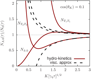
Eq. (5.66) is analogous to the ideal and first viscous correction to the thermal distribution function, $f_{0}+\delta f$, which are used in heavy ion phenomenology and in determining the shear viscosity [see for example: 75]. At large $K/k_{*}$ the distribution $N_{AA}$ attains its equilibrium value, $T(e_{0}+p_{0})/\tau$, up to viscous corrections of order $\tau_{R}/\tau$, where $\tau_{R}$ is a typical relaxation time for a mode of momentum $K$, $\tau_{R}\sim 1/\gamma_{\eta}K^{2}$.

The energy-momentum tensor averaged over fluctuations is given by

$$\langle T^{\tau\tau}\rangle =e_{0}+\frac{\langle\vec{G}^{2}\rangle}{e_{0}+p_{0}},$$ (5.67a)

$$\langle T^{xx}\rangle =p_{0}+\frac{2\eta_{0}}{3\tau}+\frac{\langle(G^{\hat{x}})^{2}\rangle}{e_{0}+p_{0}},$$ (5.67b)

$$\langle T^{yy}\rangle =p_{0}+\frac{2\eta_{0}}{3\tau}+\frac{\langle(G^{\hat{y}})^{2}\rangle}{e_{0}+p_{0}},$$ (5.67c)

$$\langle\tau^{2}T^{\eta\eta}\rangle =p_{0}-\frac{4\eta_{0}}{3\tau}+\frac{\langle(G^{\hat{z}})^{2}\rangle}{e_{0}+p_{0}}.$$ (5.67d)

Calculating $N_{ab}(\tau,{\bm{k}})=\left[(e_{A})_{a}N_{AB}(e_{B})_{b}\right]$ from the kinetic theory, we determine $\langle\phi_{a}(\tau,{\bm{k}})\phi_{b}(\tau,-{\bm{k}})\rangle$ with $\phi_{a}=\left(c_{s}\delta e,\vec{G}\right)$ in Fourier space, yielding

$$\langle\phi_{a}(x)\phi_{b}(x)\rangle ={\int}\frac{d^{2}k_{\perp}d\kappa}{(2\pi)^{3}}N_{ab}(\tau,{\bm{k}}),$$

$$={\tau}{\int}\frac{K^{2}dKd\cos\theta_{K}d\varphi_{K}}{(2\pi)^{3}}(e_{A})_{a}N_{AB}(\tau,{\bm{k}})(e_{B})_{b}\,.$$ (5.68)

Note that the momentum integral is done in final time variables, $\vec{K}(\tau)$. As shown below, the integration in Fourier space is divergent in the ultraviolet. Therefore, we regulate the integral by introducing a cutoff at $|\vec{K}|\sim\Lambda$. In turn, the background quantities such as $e_{0}$ and $\eta_{0}$ must be renormalized and depend on $\Lambda$ so that the total result is independent of $\Lambda$. The choice of $\Lambda$ is arbitrary as long as $k_{*}\ll\Lambda\ll 1/\ell_{\rm mfp}$ so that the non-linear contribution with $|\vec{K}|\sim\Lambda$ is independent of the background flow.

The integration in Eq. (5.68) includes the soft fluctuations for which the kinetic equation may not be applicable. However, this contribution is suppressed by phase space and the kinetic result can be extrapolated into this regime with negligible errors.

Combining Eqs. (5.66), (5.67) and (5.68), the energy momentum tensor is obtained as

$$\langle T^{\tau\tau}\rangle =e_{0}+3T\int_{0}^{\Lambda}\frac{K^{2}dK}{2\pi^{2}}+\Delta T^{\tau\tau},$$ (5.69a)

$$\langle T^{xx}\rangle =p_{0}+\frac{2\eta_{0}}{3\tau}+T\int_{0}^{\Lambda}\frac{K^{2}dK}{2\pi^{2}}+\frac{17}{90}\frac{T(e_{0}+p_{0})}{\eta_{0}\tau}\int_{0}^{\Lambda}\frac{dK}{2\pi^{2}}+\Delta T^{xx},$$ (5.69b)

$$\langle T^{yy}\rangle =p_{0}+\frac{2\eta_{0}}{3\tau}+T\int_{0}^{\Lambda}\frac{K^{2}dK}{2\pi^{2}}+\frac{17}{90}\frac{T(e_{0}+p_{0})}{\eta_{0}\tau}\int_{0}^{\Lambda}\frac{dK}{2\pi^{2}}+\Delta T^{yy},$$ (5.69c)

$$\langle\tau^{2}T^{\eta\eta}\rangle =p_{0}-\frac{4\eta_{0}}{3\tau}+T\int_{0}^{\Lambda}\frac{K^{2}dK}{2\pi^{2}}-\frac{17}{45}\frac{T(e_{0}+p_{0})}{\eta_{0}\tau}\int_{0}^{\Lambda}\frac{dK}{2\pi^{2}}+\tau^{2}\Delta T^{\eta\eta},$$ (5.69d)

where the finite contributions $\Delta T^{\tau\tau}$, $\Delta T^{xx}$, $\Delta T^{yy}$, and $\tau^{2}\Delta T^{\eta\eta}$ are discussed in the next section. By comparing terms with the same explicit $\tau$ dependence, the ultraviolet divergences are absorbed into the renormalized hydrodynamic variables

$$e =e_{0}(\Lambda)+\frac{T\Lambda^{3}}{2\pi^{2}},$$ (5.70a)

$$p =p_{0}(\Lambda)+\frac{T\Lambda^{3}}{6\pi^{2}},$$ (5.70b)

$$\eta =\eta_{0}(\Lambda)+\frac{17\Lambda}{120\pi^{2}}\frac{T(e_{0}(\Lambda)+p_{0}(\Lambda))}{\eta_{0}(\Lambda)}.$$ (5.70c)

Note that we do not assign a cut-off dependence to the temperature. The coefficients of the cubic and linear renormalizations of the pressure and shear viscosity are independent of the background expansion, and match the static fluid results of Sec. 5.2.2. Here $e$, $p$, and $\eta$ are physical quantities at a given temperature $T$ in an infinite volume. Using the physical quantities, the energy-momentum tensor is given as

$$\langle T^{\tau\tau}(\tau)\rangle =e+\Delta T^{\tau\tau},$$ (5.71a)

$$\langle T^{xx}(\tau)\rangle =p+\frac{2\eta}{3\tau}+\Delta T^{xx},$$ (5.71b)

$$\langle T^{yy}(\tau)\rangle =p+\frac{2\eta}{3\tau}+\Delta T^{yy},$$ (5.71c)

$$\langle\tau^{2}T^{\eta\eta}(\tau)\rangle =p-\frac{4\eta}{3\tau}+\tau^{2}\Delta T^{\eta\eta}.$$ (5.71d)

If the two-point functions of the fluctuations were completely determined by the first two terms in Eq. (5.66), their contributions would be completely absorbed by the renormalization of the background flow parameters such as $p_{0}(\Lambda)$ and $\eta_{0}(\Lambda)$. However, the kinetic equations yield residual contributions, since the full solution deviates from its asymptotic form for $K\sim k_{*}$ as seen from Fig. 5.2. The purpose of hydrodynamics with noise is to capture this contribution.

Physically, the parameters $e_{0}(\Lambda)$, $p_{0}(\Lambda)$, and $\eta_{0}(\Lambda)$ in fluctuating hydrodynamics reflect the equilibrium properties of modes above a cutoff $\Lambda$, which have been already integrated out. Equivalently, these parameters are determined by modes contained in a cell of size $a\sim 2\pi/\Lambda$. For example, $p_{0}(\Lambda)$ is the partial pressure from equilibrated modes above the cutoff (inside a cell), while the partial pressure from the modes below the cutoff (larger than a cell size) is determined dynamically with fluctuating hydrodynamics. The second terms on the right hand sides of Eq. (5.70) are the contributions to each quantity from the modes below the cutoff, when all of these long wavelength modes are in perfect equilibrium in infinite volume.

5.3.4 Out of equilibrium noise contributions to energy momentum tensor

In this section we determine the residual contributions to the energy momentum tensor, $\Delta T^{\mu\nu}$, in Eq. (5.71) after the hydrodynamic parameters have been renormalized. We evaluate the precise numerical factors of the long-time tail terms for a Bjorken expansion (which is the main result of this paper), and identify additional contributions from the noise at early times. The mathematical procedure is somewhat involved, so here we outline the calculation and present results, delegating the technical details to the Appendix 5.A.

To find the full out of equilibrium correlators we need to solve Eq. (5.65), which can be written in the following general form

$$\partial_{\tau}N_{AA}(\tau,{\bm{k}})=f(\tau,{\bm{k}})N_{AA}(\tau,{\bm{k}})+g(\tau,{\bm{k}}),$$ (5.72)

where $f(\tau,{\bm{k}})$ has contributions from both the dissipative and external forcing terms, and $g(\tau,{\bm{k}})$ is the inhomogeneous term coming from the equilibrium correlation functions. A formal solution of Eq. (5.72) is given by

$$N_{AA}(\tau,{\bm{k}}) =N_{AA}(\tau_{0},{\bm{k}})e^{\int_{\tau_{0}}^{\tau}d\tau^{\prime}f(\tau^{\prime},{\bm{k}})}+\int_{\tau_{0}}^{\tau}d\tau^{\prime\prime}g(\tau^{\prime\prime},{\bm{k}})e^{\int_{\tau_{0}}^{\tau^{\prime\prime}}d\tau^{\prime}f(\tau^{\prime},{\bm{k}})}.$$ (5.73)

The first term describes the evolution of the initial correlation density matrix $N_{AA}(\tau_{0},{\bm{k}})$ to final time $\tau$. The second term in Eq. (5.73) is the contribution from thermal fluctuations. As we will see, only the $N_{T_{1}T_{1}}$ contribution is sensitive to the initial conditions and the thermal fluctuations at early times. For the $T_{1}T_{1}$ correlator we will take the initial conditions described by Eq. (5.52) in Sec. 5.3.1, $\tau_{0}^{2}N_{T_{1},T_{1}}(\tau_{0},{\bm{k}})={\chi_{\tau_{0}}^{gg}}\,2\pi\delta(\kappa)$.

Substituting the formal solution for $N_{AA}$ in Eq. (5.67) and Eq. (5.68) we can determine the stress tensor at time $\tau\gg\tau_{0}$. The integral $\int d^{3}k$ in Eq. (5.68) diverges, but after subtracting $\Lambda^{3}$ and $\Lambda$ divergences discussed in the previous section, we finally obtain the finite correction to energy momentum tensor $\Delta T^{\mu\nu}$. Writing Eq. (5.71) in full

$$\frac{\langle\!\langle\tau^{2}T^{\eta\eta}(\tau)\rangle\!\rangle}{e+p} =\frac{p}{e+p}-\frac{4\gamma_{\eta}}{3\tau}+\frac{1.08318}{s\,(4\pi\gamma_{\eta}\tau)^{3/2}},$$ (5.74a)

$$\frac{\langle\!\langle T^{xx}(\tau)\rangle\!\rangle}{e+p} =\frac{p}{e+p}+\frac{2\gamma_{\eta}}{3\tau}+\left[\frac{{\chi_{\tau_{0}}^{gg}}{+}\delta{\chi_{\tau_{0}}^{gg}}}{\tau^{2}(e+p)^{2}}\right]\frac{1}{(12\pi\gamma_{\eta}\tau)}-\,\frac{0.273836}{s\;(4\pi\gamma_{\eta}\tau)^{3/2}},$$ (5.74b)

$$\langle\!\langle T^{yy}\rangle\!\rangle =\langle\!\langle T^{xx}\rangle\!\rangle,$$ (5.74c)

$$\langle\!\langle T^{\tau\tau}\rangle\!\rangle =\langle\!\langle T^{xx}\rangle\!\rangle+\langle\!\langle T^{yy}\rangle\!\rangle+\langle\!\langle\tau^{2}T^{\eta\eta}\rangle\!\rangle.$$ (5.74d)

The coefficients $1.08318$ and $-0.273836$ of the long-time tails, $1/(\gamma_{\eta}\tau)^{3/2}$ are obtained by numerical integration as explained in Appendix 5.A. The term ${\chi_{\tau_{0}}^{gg}}+\delta{\chi_{\tau_{0}}^{gg}}$ records the initial variance in transverse momentum in a given rapidity slice (see Eq. (5.46) and Eq. (5.48)) together with the thermal contribution

$${\chi_{\tau_{0}}^{gg}}{+}\delta{\chi_{\tau_{0}}^{gg}}=\left\langle\frac{1}{{\mathcal{A}}}\left(\frac{dp^{x}}{d\eta}\right)^{\!2}\right\rangle_{\!\!\tau_{0}}+\left(\frac{T(e+p)\tau_{0}}{\sqrt{12\pi\gamma_{\eta}/\tau_{0}}}\right)_{\!\tau_{0}},$$ (5.75)

where the brackets $\left(\ldots\right)_{\tau_{0}}$ indicate that all contained quantities are to be evaluated at the initial time, $\tau_{0}$. We will provide an intuitive discussion of the result in the next section.

5.3.5 Qualitative discussion of Eq. (5.74)

Long time tails: $1/(\gamma_{\eta}\tau)^{3/2}$

Examining Eq. (5.74) we see two groups of terms. The first group is proportional to $1/(\gamma_{\eta}\tau)^{3/2}$ and is independent of initial conditions. By contrast, the second group is proportional to $1/(\gamma_{\eta}\tau)$, and depends on the initial transverse momentum fluctuations through the parameter ${\chi_{\tau_{0}}^{gg}}+\delta{\chi_{\tau_{0}}^{gg}}$ (see Sec. 5.3.1). We will first describe the terms proportional to the fractional power $1/(\gamma_{\eta}\tau)^{3/2}$, known as the long-time tails.

Squared fluctuations in equilibrium are of order $\langle\delta e(\vec{x})\delta e(\vec{y})\rangle_{\rm eq}/e^{2}\sim\langle v^{i}(\vec{x})v^{j}(\vec{y})\rangle_{\rm eq}\sim s^{-1}\delta(\vec{x}-\vec{y})$, where $s$ is the entropy density (see Eq. (5.4)). Thus a fluctuation with wavenumber $k$ is suppressed by $\sqrt{k^{3}/s}$. The suppression factor $k^{3}/s$ is roughly the inverse of the degrees of freedom inside a box of volume $\Delta V\sim(1/k)^{3}$, which must be a huge number for local thermodynamics to apply. This is why the linear analysis of the hydrodynamic fluctuations is justified.

The energy momentum tensor in viscous hydrodynamics is expanded in powers of gradients, leading to corrections in powers of $\epsilon\equiv\eta/(e+p)\tau\ll 1$. In addition, as discussed in Sec. 5.1.2 the fluctuations with wavenumber of order $|\vec{K}|\sim k_{*}\sim 1/(\gamma_{\eta}\tau)^{1/2}$ dominate the nonlinear noise correction to the stress tensor, which is suppressed by $s\Delta V\equiv s/k_{*}^{3}\gg 1$. This correction to the longitudinal pressure reflects the equipartition of energy, with $\tfrac{1}{2}T$ of energy per mode, and the number of non-equilibrium modes per volume $\sim k_{*}^{3}$. To summarize, the reasoning in this paragraph leads to the following parametric estimate for the longitudinal stress

$$\frac{\langle\tau^{2}T^{\eta\eta}\rangle}{e+p}\sim\left[\frac{1}{4}+\frac{\eta}{(e+p)\tau}+\frac{1}{s(\gamma_{\eta}\tau)^{3/2}}+\cdots\right],$$ (5.76)

which is reflected by Eq. (5.74).

Transverse momentum diffusion in rapidity: $1/\gamma_{\eta}\tau$

Additional corrections to the stress in Eq. (5.74) decrease as $1/\gamma_{\eta}\tau$, in contrast to the long time tails. As described in Sec. 5.3.1, long range (in rapidity) initial transverse momentum fluctuations correct the mean transverse pressures, $T^{xx}$ and $T^{yy}$, by a term proportional to ${\chi_{\tau_{0}}^{gg}}/\gamma_{\eta}\tau$ (see Eq. (5.74b)). Hydrodynamic noise in the initial state adjusts this correction by adding to the long range fluctuations of transverse momentum (see Eqs. (5.74b) and (5.75)). The goal of this section is to explain this process qualitatively, and to quantitatively explain the adjustment, ${\chi_{\tau_{0}}^{gg}}\rightarrow{\chi_{\tau_{0}}^{gg}}+\delta{\chi_{\tau_{0}}^{gg}}$.

Formally, the $N_{T_{1}T_{1}}$ correlation function is sensitive to the noise at the initial time $\tau_{0}$, which arises from a restricted region of $\vec{K}$-space integration, $k_{\perp}\sim k_{*}$ and $\kappa/\tau\sim k_{*}(\tau_{0})(\tau_{0}/\tau)\sim k_{*}(\tau_{0}/\tau)^{1/3}\ll k_{*}$. In this region the longitudinal momentum $\kappa/\tau_{0}$ reflects the dissipative scale $k_{*}(\tau_{0})$ at the initial time $\tau_{0}$, while the transverse momenta reflect the dissipative scale at final time $\tau$.

The dynamics in this phase space region is the following. During the initial moments, thermal fluctuations lead to a local fluctuation of transverse momentum in a given rapidity slice for each cell in the transverse plane

$$\left\langle(\tau_{0}\Delta g^{x}_{\perp})^{2}\right\rangle\sim\left(\frac{T\,(e+p)\,\tau_{0}}{\Delta\eta\,(\Delta x_{\perp})^{2}}\right)_{\tau_{0}}.$$ (5.77)

Here (as before) the brackets $(\ldots)_{\tau_{0}}$ indicate that all contained quantities should be evaluated at $\tau_{0}$. During an initial time of order $\tau_{0}$, the momentum per rapidity diffuses to a finite longitudinal width [184] (see below)

$$\Delta\eta\rightarrow\sigma_{\eta}(\tau_{0})\equiv\sqrt{6\gamma_{\eta}(\tau_{0})/\tau_{0}}.$$ (5.78)

The process is diffusive because the transverse momentum per rapidity is conserved. The rapidity width is finite because the longitudinal expansion shuts off the diffusion process. $\sigma_{\eta}(\tau_{0})$ is broader than the rapidity width of subsequent interest, which is of order $\sigma_{\eta}(\tau)$. Thus, after an initial transient, the transverse momentum per rapidity may be considered approximately constant in time and rapidity, though localized in this transverse plane

$$\left\langle(\tau\Delta g^{x}_{\perp})^{2}\right\rangle\sim\left(\frac{T\,(e+p)\,\tau_{0}}{\sqrt{\gamma_{\eta}/\tau_{0}}}\right)_{\tau_{0}}\frac{1}{(\Delta x_{\perp})^{2}}.$$ (5.79)

At much later times these transverse momentum fluctuations diffuse transversely (as described in Sec. 5.3.1) leading to a correction of order

$$\frac{\left\langle T^{xx}\right\rangle}{e+p}\sim\frac{1}{\tau^{2}(e+p)^{2}}\left(\frac{T(e+p)\tau_{0}}{\sqrt{\gamma_{\eta}/\tau_{0}}}\right)_{\tau_{0}}\frac{1}{\gamma_{\eta}\tau},$$ (5.80)

which qualitatively reproduces the correction in Eq. (5.74b).

Now we will briefly sketch this reasoning with equations. At the early time moments $\tau\sim\tau_{0}$, the wave vector is predominantly longitudinal $\vec{K}\simeq(\vec{0}_{\perp},\kappa/\tau)$ and the transverse momentum correlator

$$\left\langle g^{i}_{\perp}(\tau,{\bm{k}})g^{j}_{\perp}(\tau,-{\bm{k}}^{\prime})\right\rangle\equiv N^{ij}({\bm{k}},\tau)(2\pi)^{3}\delta^{3}({\bm{k}}-{\bm{k}}^{\prime}),$$ (5.81)

can be reconstructed from $N_{T_{1}T_{1}}$ and $N_{T_{2}T_{2}}$

$$N^{ij}(\tau,{\bm{k}})=\sum_{A\in T_{1},T_{2}}e_{A}^{i}e_{A}^{j}N_{AA}(\tau,{\bm{k}}),$$ (5.82)

since $\vec{T}_{1}$ and $\vec{T}_{2}$ form a basis for the transverse plane. In this limit, the equations of motion for $N_{T_{1}T_{1}}$ and $N_{T_{2}T_{2}}$ (see Eq. (5.65b) and Eq. (5.65c)) are the same, and $N^{ij}$ satisfies a one dimensional diffusion equation with a source at early times

$$\left(\partial_{\tau}+2\gamma_{\eta}\left(\frac{\kappa}{\tau}\right)^{2}\right)(\tau^{2}N^{ij})=2\gamma_{\eta}\left(\frac{\kappa}{\tau}\right)^{2}\,T(e+p)\tau\delta^{ij}\,.$$ (5.83)

The lhs of Eq. (5.83) represents the diffusion of transverse momentum in rapidity, while the rhs represents the thermal transverse momentum fluctuations at the earliest moments, which act as a source. The source for the fluctuations, $2T\eta\,(\kappa/\tau)^{2}$, is a rapidly decreasing function of time, and is dominant for times of order $\tau_{0}$.

The Green function propagating data from $\tau^{\prime}$ to $\tau$ for the lhs of Eq. (5.83) is

$$G^{ij}(\tau\eta{\vec{x}_{\perp}}|\tau^{\prime}\eta^{\prime}{\vec{x}_{\perp}}^{\prime}){=}\frac{e^{-(\eta-\eta^{\prime})^{2}/(12\gamma_{\eta}(\tau^{\prime})/\tau^{\prime})}}{\sqrt{12\pi\gamma_{\eta}(\tau^{\prime})/\tau^{\prime}}}\delta^{ij}\delta^{2}({\vec{x}_{\perp}}-{\vec{x}_{\perp}}^{\prime}),$$ (5.84)

for $\tau\gg\tau^{\prime}$. Thus, a fluctuation localized in rapidity at time $\tau_{0}$ will diffuse to a finite rapidity width of $\sigma_{\eta}(\tau_{0})=\sqrt{6\gamma_{\eta}(\tau_{0})/\tau_{0}}$ at late times [184, 233]. This is a small rapidity width in absolute units (since $\gamma_{\eta}(\tau_{0})/\tau_{0}\ll 1$ when hydrodynamics is a good approximation), but much broader than the rapidity width of interest at the final time, $\gamma_{\eta}(\tau_{0})/\tau_{0}\gg\gamma_{\eta}(\tau)/\tau$.

Returning to Eq. (5.83), we solve the equation, and determine the transverse momentum correlation function (in the same rapidity slice) at an intermediate time $\tau^{\prime}$ which is large compared to $\tau_{0}$ but much much less than the final time $\tau$, $\tau_{0}\ll\tau^{\prime}\ll\tau$

$$\tau^{\prime 2}\left\langle g^{i}_{\perp}(\tau^{\prime},\eta,{\vec{x}_{\perp}})g^{j}_{\perp}(\tau^{\prime},\eta,{\vec{y}_{\perp}})\right\rangle=\int\frac{d\kappa d^{2}k_{\perp}}{(2\pi)^{3}}e^{i\vec{k}_{\perp}\cdot({\vec{x}_{\perp}}-{\vec{y}_{\perp}})}\;\tau^{\prime 2}N^{ij}(\tau^{\prime},\kappa)\,.$$ (5.86)

Implementing these steps we find

$$\tau^{\prime 2}\left\langle g^{i}_{\perp}(\tau^{\prime},\eta,{\vec{x}_{\perp}})g^{j}_{\perp}(\tau^{\prime},\eta,{\vec{y}_{\perp}})\right\rangle=\left(\frac{T(e+p))\tau_{0}}{\sqrt{12\pi\gamma_{\eta}/\tau_{0}}}\right)_{\!\!\tau_{0}}\!\!\delta^{ij}\delta^{2}({\vec{x}_{\perp}}-{\vec{y}_{\perp}}).$$ (5.87)

This has the same form as the initial conditions described in Sec. 5.3.1, and fluctuations at the earliest moments simply increase the variance of long range transverse momentum fluctuations by a constant amount

$$\delta{\chi_{\tau_{0}}^{gg}}=\left(\frac{T(e+p)\tau_{0}}{\sqrt{12\pi\gamma_{\eta}/\tau_{0}}}\right)_{\!\tau_{0}},$$ (5.88)

reproducing Eq. (5.75). In a sense, this constant shift simply finalizes the thermalization process described at the start of Sec. 5.3.1. The correction $\delta{\chi_{\tau_{0}}^{gg}}$ scales as $\tau_{0}^{-1/3}$ and is therefore small compared to the first term in Eq. (5.75) if $\tau_{0}$ is large compared to a typical thermalization time.

5.4 Results and Discussion

In this paper we determined a set of kinetic equations which describe the evolution of hydrodynamic fluctuations during a Bjorken expansion. We used these equations to find the first fractional power correction to the longitudinal pressure, $\propto 1/(\tau T)^{3/2}$, at late times. The evolution equations can be extended to much more general flows, and ultimately coupled to existing hydrodynamic codes.

The kinetic equations for hydrodynamic fluctuations are a WKB (or rotating wave) type approximation of the full stochastic hydrodynamic evolution equations. This approximation is justified because the relevant hydrodynamic modes have wavenumbers of order

$$k_{*}\sim\sqrt{\frac{e+p}{\eta\tau}}\,,$$ (5.89)

which is large compared to the inverse expansion rate, $1/\tau$. For example, the kinetic equation for the sound mode with wavenumber $\vec{K}=(\vec{k}_{\perp},\kappa/\tau)$ interacting with the Bjorken background takes the form of a relaxation type equation

$$\partial_{\tau}N_{++}(\tau,{\bm{k}})=-\frac{4}{3}\gamma_{\eta}K^{2}\left[N_{++}-\frac{T(e_{0}+p_{0})}{\tau}\right]-\frac{1}{\tau}\left(2+c_{s}^{2}+\cos\theta_{K}\right)N_{++}\,.$$ (5.90)

$N_{++}(\tau,{\bm{k}})$ are short wavelength (symmetrized) two point functions of conserved stress tensor components, $\phi_{+}\equiv(c_{s}\delta e+\hat{K}\cdot\vec{G})/\sqrt{2}$ in an evolving Bjorken hydrodynamic background (see Sec. 5.3 and Eq. (5.65) for the remaining modes). At high wavenumbers $K\gg k_{*}$, the distribution function $N_{++}$ reaches its equilibrium form $T(e_{0}+p_{0})/\tau$, up to first viscous corrections which may be found by solving Eq. (5.90) order by order at large $K/k_{*}$ (see Eq. (5.66a)). This asymptotic form is responsible for the renormalization of the pressure and shear viscosity. For wavenumbers of order $k_{*}$ the hydrodynamic fluctuations are not in equilibrium at all, but reach a non-equilibrium steady state at late times. A graph of this non-equilibrium steady state is given in Fig. 5.2.

The deviation of hydrodynamic fluctuations from equilibrium has consequences for the evolution of the system. Indeed, the longitudinal pressure $\tau^{2}T^{\eta\eta}$ receives a correction from the unequilibrated modes

$$\frac{\left\langle\tau^{2}T^{\eta\eta}\right\rangle}{e+p}=\Big{[}\frac{p}{e+p}-\frac{4}{3}\frac{\gamma_{\eta}}{\tau}+\frac{1.08318}{s\,(4\pi\gamma_{\eta}\tau)^{3/2}}+\frac{(\lambda_{1}-\eta\tau_{\pi})}{e+p}\frac{8}{9\tau^{2}}\Big{]}\,,$$ (5.91)

where we have repeated Eq. (5.74a) for convenience. The correction to the pressure ${\sim}T/(\gamma_{\eta}\tau)^{3/2}$ is of order ${\sim}Tk_{*}^{3}$, reflecting the number of modes of order $k_{*}$ and the energy per mode, $\tfrac{1}{2}T$. In contrast to all previous analyses of long-time tails [183, 182], the hydrodynamic fluctuations in the expanding case are not close to equilibrium, and a one loop expansion around equilibrium is not an appropriate approximation scheme. Our kinetic description effectively resums all diagrams contributing at the same order in the presence of expansion [232].

Formally, the noise correction is lower order than the correction due to second order hydrodynamics, which is proportional to a particular combination of second order parameters, $\lambda_{1}-\eta\tau_{\pi}$. To quantify the importance of thermal fluctuations in practice, we take representative numbers for the entropy from the lattice [234, 116], estimates for the second order hydrodynamic coefficients based on weakly and strongly coupled plasmas [209, 115, 114], and an estimate for $\tau T$ at $\tau\sim 3.5\,{\rm fm}$ based on hydrodynamic simulations

$$\frac{T^{3}}{s}\simeq \frac{1}{13.5}\,,$$ (5.92a)

$$\frac{(\lambda_{1}-\eta\tau_{\pi})}{e+p}\simeq -0.8\left(\frac{\eta}{e+p}\right)^{2}\,,$$ (5.92b)

$$\tau T\simeq 4.5\,.$$ (5.92c)

Then, for $\eta/s\simeq 1/4\pi$, Eq. (5.91) evaluates to

$$\frac{\left\langle\tau^{2}T^{\eta\eta}\right\rangle}{e+p}=\frac{1}{4}\Big{[}1.-0.092\,\left(\frac{4.5}{\tau T}\right)+0.034\,\left(\frac{4.5}{\tau T}\right)^{3/2}-0.00085\left(\frac{4.5}{\tau T}\right)^{2}\Big{]},$$ (5.93)

while for $\eta/s=2/4\pi$, we find

$$\frac{\left\langle\tau^{2}T^{\eta\eta}\right\rangle}{e+p}=\frac{1}{4}\Big{[}1.-0.185\left(\frac{4.5}{\tau T}\right)+0.013\left(\frac{4.5}{\tau T}\right)^{3/2}-0.0034\left(\frac{4.5}{\tau T}\right)^{2}\Big{]}.$$ (5.94)

For the smaller shear viscosity, Eq. (5.93), the nonlinear noise contribution completely dominates over the second order hydro contribution. For the larger shear viscosity, Eq. (5.94), the noise remains three times larger than second order hydro, but this contribution is only a $\sim 10\%$ of the first order viscous term. Finally, for $\eta/s\sim 3/4\pi$ the noise and second order hydro contributions become comparable.

The evolution of the average energy density of the system obeys

$$\frac{d\langle\!\langle T^{\tau\tau}\rangle\!\rangle}{d\tau}=-\frac{\langle\!\langle T^{\tau\tau}\rangle\!\rangle+\langle\!\langle\tau^{2}T^{\eta\eta}\rangle\!\rangle}{\tau},\ \ \$$ (5.95)

where the double brackets notate an average over (long range in rapidity) initial conditions and thermal noise. To close the system of equations, the relationship between average energy density $\langle\!\langle T^{\tau\tau}\rangle\!\rangle$ and the average rest frame energy density $e(\tau)$ must be specified, and this relation is given in Eq. (5.74). $T^{\tau\tau}$, $T^{xx}$, and $T^{yy}$ are sensitive to hydrodynamic noise at the earliest moments in addition to the long-time tails. In these cases thermal noise in the initial state adds to the long-range rapidity correlation functions of transverse momentum, which are already present without noise. This result is encapsulated by Eq. (5.75) and is discussed in Sec. 5.3.1 and Sec. 5.3.5.

Although the analysis of hydrodynamic fluctuations in this paper was limited to conformal neutral fluids and a Bjorken expansion, the techniques developed here can be applied to much more general flows. A next step is to generalize the kinetic equations in Eq. (5.65) to an arbitrary expansion, and to couple such generalized equations to existing second order hydrodynamic codes. In addition, it will be phenomenologically important to extend this work to non-conformal systems with net baryon number. Near the QCD critical point the noise will continue to grow without bound, leading to a critical renormalization of the bulk viscosity. In an expanding system these fluctuations will not be fully equilibrated. We believe the formalism set up in this paper provides the first steps towards quantitatively analyzing this rich dynamical regime.

Appendices

Appendix 5.A Computation of finite residual contributions

In this appendix we provide the details of the computation sketched in Sec. 5.3.4 for the residual out of equilibrium noise contribution to the energy momentum tensor for a Bjorken background. Let us scale the correlation density matrix by the equilibrium value:

$$R_{AA}(\tau,{\bm{k}})\equiv\frac{N_{AA}(\tau,{\bm{k}})}{T(e_{0}+p_{0})/\tau}.$$ (5.96)

The kinetic equations of motion Eq. (5.65) written for relative density matrix $R_{AA}$ are

$$\partial_{\tau}R_{\pm\pm} =-\frac{4}{3}\gamma_{\eta}K^{2}\left(R_{\pm\pm}-1\right)+\frac{c_{s}^{2}-\cos^{2}\theta_{K}}{\tau}R_{\pm\pm},$$ (5.97)

$$\partial_{\tau}R_{T_{1}T_{1}} =-2\gamma_{\eta}K^{2}\left(R_{T_{1}T_{1}}-1\right)+\frac{2c_{s}^{2}}{\tau}R_{T_{1}T_{1}},$$ (5.98)

$$\partial_{\tau}R_{T_{2}T_{2}} =-2\gamma_{\eta}K^{2}\left(R_{T_{2}T_{2}}-1\right)+\frac{2(c_{s}^{2}-\sin^{2}\theta_{K})}{\tau}R_{T_{2}T_{2}}.$$ (5.99)

Using dimensionless variables $t\equiv\tau^{\prime}/\tau$ and $\vec{r}\equiv\vec{K}/k_{*}$ with $\vec{K}=(\vec{k}_{\perp},\kappa/\tau)$ and $k_{*}=1/(\gamma_{\eta}\tau)^{1/2}$ defined at $\tau$, the Green functions for the homogeneous parts are

$$G_{\pm\pm}(\tau^{\prime},\tau;{\bm{k}}) =\frac{1}{t^{c_{s}^{2}}}\frac{1}{\sqrt{A(t,\theta_{K})}}\exp\left[-\frac{4}{3}r^{2}B(t,\theta_{K})\right],$$ (5.100)

$$G_{T_{1}T_{1}}(\tau^{\prime},\tau;{\bm{k}}) =\frac{1}{t^{2c_{s}^{2}}}\exp\left[-2r^{2}B(t,\theta_{K})\right],$$ (5.101)

$$G_{T_{2}T_{2}}(\tau^{\prime},\tau;{\bm{k}}) =t^{2-2c_{s}^{2}}A(t,\theta_{K})\exp\left[-2r^{2}B(t,\theta_{K})\right],$$ (5.102)

where

$$A(t,\theta_{K}) \equiv\sin^{2}\theta_{K}+\frac{\cos^{2}\theta_{K}}{t^{2}},$$ (5.103)

$$B(t,\theta_{K}) \equiv\frac{\sin^{2}\theta_{K}}{1+c_{s}^{2}}\left(1-t^{1+c_{s}^{2}}\right)+\frac{\cos^{2}\theta_{K}}{1-c_{s}^{2}}\left(\frac{1}{t^{1-c_{s}^{2}}}-1\right).$$ (5.104)

With these Green functions, $R_{AA}$ due to thermal fluctuations (in contrast to initial fluctuations discussed in Sec. 5.3.1) is given by

$$R_{++}(\tau,{\bm{k}}) =\int_{\tau_{0}}^{\tau}d\tau^{\prime}\frac{4}{3}\gamma_{\eta}(\tau^{\prime})\left(k_{\perp}^{2}+\frac{\kappa^{2}}{\tau^{\prime 2}}\right)G_{++}(\tau^{\prime},\tau;{\bm{k}}),$$ (5.105)

and similarly for the other modes (change 4/3 to 2 for the transverse modes). Since the asymptotic solution of $R_{AA}$ for large $K$ is known, we define the remainder of $R_{AA}$ as:

$$R^{(\rm r)}_{\pm\pm}(\tau,{\bm{k}}) \equiv R_{\pm\pm}(\tau,{\bm{k}})-\left(1+\frac{c_{s}^{2}-\cos^{2}\theta_{K}}{\frac{4}{3}\gamma_{\eta}K^{2}\tau}\right),$$ (5.106)

$$R^{(\rm r)}_{T_{1}T_{1}}(\tau,{\bm{k}}) \equiv R_{T_{1}T_{1}}(\tau,{\bm{k}})-\left(1+\frac{c_{s}^{2}}{\gamma_{\eta}K^{2}\tau}\right),$$ (5.107)

$$R^{(\rm r)}_{T_{2}T_{2}}(\tau,{\bm{k}}) \equiv R_{T_{2}T_{2}}(\tau,{\bm{k}})-\left(1+\frac{c_{s}^{2}-\sin^{2}\theta_{K}}{\gamma_{\eta}K^{2}\tau}\right).$$ (5.108)

Using $R_{AA}^{(\rm r)}$ the residual contribution to the energy-momentum tensor is calculated from Eq. (5.67a) and Eq. (5.68) as

$$\Delta T^{xx} =T\int\frac{d^{3}K}{(2\pi)^{3}}\left[\begin{aligned} &\frac{R^{(\rm r)}_{++}+R^{(\rm r)}_{--}}{2}\sin^{2}\theta_{K}\cos^{2}\varphi_{K}\\ &+R^{(\rm r)}_{T_{1}T_{1}}\sin^{2}\varphi_{K}\\ &+R^{(\rm r)}_{T_{2}T_{2}}\cos^{2}\theta_{K}\cos^{2}\varphi_{K}\end{aligned}\right],$$ (5.109)

$$\Delta T^{yy} =T\int\frac{d^{3}K}{(2\pi)^{3}}\left[\begin{aligned} &\frac{R^{(\rm r)}_{++}+R^{(\rm r)}_{--}}{2}\sin^{2}\theta_{K}\sin^{2}\varphi_{K}\\ &+R^{(\rm r)}_{T_{1}T_{1}}\cos^{2}\varphi_{K}\\ &+R^{(\rm r)}_{T_{2}T_{2}}\cos^{2}\theta_{K}\sin^{2}\varphi_{K}\end{aligned}\right],$$ (5.110)

$$\tau^{2}\Delta T^{\eta\eta} =T\int\frac{d^{3}K}{(2\pi)^{3}}\left[\begin{aligned} &\frac{R^{(\rm r)}_{++}+R^{(\rm r)}_{--}}{2}\cos^{2}\theta_{K}\\ &+R^{(\rm r)}_{T_{2}T_{2}}\sin^{2}\theta_{K}\end{aligned}\right],$$ (5.111)

$$\Delta T^{\tau\tau} =\Delta T^{xx}+\Delta T^{yy}+\tau^{2}\Delta T^{\eta\eta}.$$ (5.112)

Substituting the subtracted solution $R^{(\rm r)}_{AA}$ into (5.109)-(5.112) and performing $r$ integration with a Gaussian cutoff $\exp[-r^{2}k_{*}^{2}/\Lambda^{2}]$, we get

$$\frac{\left[\tau^{2}\Delta T^{\eta\eta}(\tau)\right]}{T(\tau)k_{*}^{3}}=\frac{3\sqrt{\pi}}{8}\int_{-1}^{1}\frac{d(\cos\theta_{K})}{4\pi^{2}}\int_{\tau_{0}/\tau\to 0}^{1}dt$$

$$\ \ \ \times\left(\frac{\frac{4}{3}\cos^{2}\theta_{K}\sqrt{A(t,\theta_{K})}}{\left[\frac{4}{3}B(t,\theta_{K})+k_{*}^{2}/\Lambda^{2}\right]^{5/2}}+\frac{2t^{2-c_{s0}^{2}}\sin^{2}\theta_{K}A(t,\theta_{K})^{2}}{\left[2B(t,\theta_{K})+k_{*}^{2}/\Lambda^{2}\right]^{5/2}}\right)$$

$$\ \ \ -\left[\mathcal{O}(\Lambda^{3})+\mathcal{O}(\Lambda)\right],$$ (5.113)

$$\frac{\left[\Delta T^{xx}(\tau)+\Delta T^{yy}(\tau)\right]}{T(\tau)k_{*}^{3}}=\frac{3\sqrt{\pi}}{8}\int_{-1}^{1}\frac{d(\cos\theta_{K})}{4\pi^{2}}\int_{\tau_{0}/\tau}^{1}dt$$

$$\ \ \ \ \ \ \times\left(\frac{\frac{4}{3}\sin^{2}\theta_{K}\sqrt{A(t,\theta_{K})}}{\left[\frac{4}{3}B(t,\theta_{K})+k_{*}^{2}/\Lambda^{2}\right]^{5/2}}\right.$$

$$\ \ \ \ \ \ \ \ \ \ \ \left.+\ \frac{2t^{2-c_{s}^{2}}\cos^{2}\theta_{K}A(t,\theta_{K})^{2}+2t^{-c_{s}^{2}}A(t,\theta_{K})}{\left[2B(t,\theta_{K})+k_{*}^{2}/\Lambda^{2}\right]^{5/2}}\right)$$

$$\ \ \ \ \ -\left[\mathcal{O}(\Lambda^{3})+\mathcal{O}(\Lambda)\right]$$ (5.114)

The ultraviolet divergent terms $\mathcal{O}(\Lambda^{3},\Lambda)$ are from the asymptotic form of $R_{AA}$ at large $K$ in (5.106)-(5.108). Near $t=1$, $B(t,\theta_{K})\simeq 1-t$ and the cutoff $\Lambda$ regulates the divergence in time integral. To isolate the divergences, we perform the partial integration twice and pick up cubic and linear divergences from the surface terms at $t=1$. The resultant divergences are precisely canceled by $\mathcal{O}(\Lambda^{3},\Lambda)$ terms.

After subtracting the ultraviolet divergences at $t=1$ and doing $\cos\theta_{K}$ integral analytically, the remaining time integration has to be done numerically. $R^{(\rm r)}_{T_{1}T_{1}}$ mode contribution to $T^{xx}$ and $T^{yy}$ is divergent in the limit $\tau\gg\tau_{0}$. Since the analytic behavior of the integrand around $t\sim 0$ is known, we can explicitly subtract the part sensitive to early times from the integrand to extract remaining finite pieces for $R^{(\rm r)}_{T_{1}T_{1}}$ mode. Numerical integration results necessary to find finite stress tensor corrections in Eqs. (5.109)-(5.111) are summarized in Table 5.1. Summing contributions from the different modes to the longitudinal and transverse components of energy momentum tensor gives the numerical coefficients $1.08318$ and $-0.273836$ as seen in Eq. (5.74).

$\begin{array}[]{|c|c|c|}\hline\cr R^{(\rm r)}_{AA}&(4\pi)^{-3/2}\int d^{3}rR^{(\rm r)}_{AA}&(4\pi)^{-3/2}\int d^{3}r\cos^{2}\theta_{K}R^{(\rm r)}_{AA}\\ \hline\cr R^{(\rm r)}_{\pm\pm}&-0.439511&0.021281\\ R^{(\rm r)}_{T_{1}T_{1}}&-\frac{\pi}{3\sqrt{6}}\approx-0.427517&-0.467513\\ R^{(\rm r)}_{T_{2}T_{2}}&1.402539&0.340636\\ \hline\cr\end{array}$

Table 5.1: Numerical values of finite pieces of regularized $R^{(\rm r)}_{AA}$ integrals for energy momentum tensor corrections. For the special case of $\int d^{3}rR^{(\rm r)}_{T_{1}T_{1}}$ the remaining one dimensional time integral can be done analytically.

Chapter 6 Conclusion

Fluctuations in heavy ion collisions are the key experimental observables, and therefore a sophisticated understanding of perturbations is necessary for the precision extraction of the bulk properties of the Quark Gluon Plasma (QGP). In this dissertation I discussed my work [1, 2, 3, 4] on the evolution of initial, pre-equilibrium, and thermal fluctuations in heavy ion collisions.

In Chapter 3 I used Principal Component Analysis (PCA) to study the initial fluctuations in hydrodynamic simulations of heavy ion collisions at the CERN Large Hadron Collider (LHC) (${\sqrt{s_{\scriptscriptstyle NN}}}=2.76\,\text{TeV}$). In particular, I explicitly showed that factorization breaking of momentum dependent flow harmonics $v_{n}(p_{T})$ (where $n=0\text{--}5$) can be quantitatively characterized by the interplay of subleading flows, which have an intuitive physical interpretation. For the $n=0,1,3$ harmonics the subleading flow is a response to the radial excitation of the $n$th order eccentricity $\varepsilon_{n}$. In contrast, for the $n=2,4,5$ harmonics a nonlinear mixing plays an important part in generating subleading components. For example, in the case of the $n=2$ harmonic in peripheral collisions, the large leading elliptic flow $v_{2}$ mixes with the radial flow $v_{0}$ fluctuations and produces a new subleading elliptic flow. Correctly identifying different sources of flow helps finding the optimal geometric and nonlinear predictors for the flow harmonics. The main message of this work is that the momentum dependent harmonic flow $v_{n}(p_{T})$ should be thought of not as a single response to a coarse grained initial state quantity, like $\varepsilon_{n}$, but a superposition of responses to various aspects of the initial state geometry. The tools described in Chapter 3 give the most systematic way to date of unraveling the map between initial state fluctuations and the final state flow.

The PCA is a systematic and efficient way of decomposing flow into its most significant components. Importantly, studying the two-particle correlation functions in terms of dominant principal components utilizes all correlation data. Because subleading flows are more sensitive to the finer radial structure of the initial geometry, the subleading flows are an additional way of constraining the heavy ion collision models with already measured data. Subleading flows could also help interpreting some flow features in the ultra-central Pb+Pb collisions, which are not yet reproduced by simulations [235]. The PCA is a universal statistical method and can be used for disentangling correlations in rapidity $\eta$, where our understanding of fluctuations is still developing [160]. Finally, because the full two-particle correlation matrix is very well described by just two or three principle components, the correct physical interpretation and quantitative reproduction of the leading principal components is a thorough test of our understanding of the QGP expansion.

In Chapter 4 I looked at the equilibration of initial state fluctuations at the early stages of heavy ion collisions using the framework of weakly coupled kinetic theory [100, 140]. Kinetic theory at realistic values of the coupling constant $\alpha_{s}\approx 0.26$ (which is outside the strict weak coupling regime) predicts phenomenologically feasible (i.e. short enough) equilibration time of a uniform background [169]. In this work, I demonstrated that transverse perturbations in the initial state also approach hydrodynamics at the same time. Furthermore, the entire kinetic pre-thermal evolution can be conveniently expressed in Green functions which map transverse perturbations in the initial state to energy momentum tensor at the time when hydrodynamics becomes applicable. Importantly, because the pre-thermal evolution time is short, it is enough to study equilibration within a causal region which is much smaller than the total transverse nuclear geometry.

Effective kinetic theory provides a first principle QCD description of the QGP equilibration and naturally connects the weak coupling initial state models like IP-Glasma to hydrodynamics—a connection which was so far missing. However, at the relevant energy scales in heavy ion collisions the coupling constant $\alpha_{s}\sim 0.3$ is not in the asymptotically weak coupling regime $\alpha_{s}\ll 1$ and the extrapolated kinetic theory results should be taken cautiously. The kinetic theory domain of validity can be extended by non-perturbative treatment of soft momentum physics, e.g. non-perturbative anisotropic screening [153, 154, 155]. In a tangential development, the current work can be straightforwardly extended to study the chemical equilibration of quarks and gluons, and the production of out-of-equilibrium thermal photons.

The rapid equilibration in heavy ion collisions is a poorly understood problem, which is even more acute for small collision systems with very short lifetimes. Although the exact nature of equilibration is yet to be seen, the short evolution time and causality constrain the possible forms of response functions. Therefore an effective description can perhaps be inferred from the interpolation between the weak coupling theory and models based on holography that describe equilibration at infinitely strong coupling in QCD-like theories [170]. In fact, out-of-equilibrium quantum systems demonstrate surprisingly universal behavior in very different settings [152, 236, 237]. The kinetic theory response functions computed in this work represents a practical implementation of the “bottom-up” thermalization scenario and is the first work directly connecting “bottom-up” to current hydrodynamic models of heavy ion collisions.

Finally, in Chapter 5 I addressed the physics of thermal fluctuations in the hydrodynamically expanding QGP by constructing the effective hydro-kinetic equations for the two-point correlation function. The rapid Bjorken expansion of a medium drives the hydrodynamic fluctuations out of equilibrium prescribed by the fluctuation-dissipation theorem. The competition between the expansion and dissipation leads to a steady state solution of hydro-kinetic equations. The difference between the equilibrium correlations and the steady state solution determines the so called “long time tail” corrections to the energy momentum tensor, however the exact numerical factors for Bjorken expanding background were calculated here for the first time. The separation of scales between the long wavelength background physics and the dominant out-of-equilibrium hydrodynamic fluctuations gives an intuitive picture for the nonlinear noise contributions.

The estimated nonlinear noise corrections in heavy ion collisions are potentially as large or larger than second order terms used in the modern hydrodynamic models and the presented framework of hydro-kinetic equations is an alternative to numerically challenging stochastic hydrodynamic simulations. More importantly, the hydro-kinetic equations are a leading order effective kinetic theory of noise and can be used to give a perturbative description of noise away from the QCD critical point. The framework can be straightforwardly applied to general background flows and non-conformal systems with non-vanishing bulk viscosity.

In summary, in this dissertation I discussed and applied several methods of separating and propagating initial and thermal fluctuations in heavy ion collisions: Principal Component Analysis, kinetic theory equilibration, and hydro-kinetic equations of noise. The high energy Pb+Pb and Au+Au collisions at LHC and RHIC are likely to remain the most reliable grounds for determining QCD medium properties, but collisions in small systems (e.g. p+Pb or high multiplicity p+p) exhibit surprisingly similar signals of collectivity. Principal Component Analysis and kinetic theory equilibration are promising tools to study initial fluctuations in these systems. On the other hand, the Beam Energy Scan will search for the QCD critical point in the low energy and high baryon chemical potential region of the QCD phase diagram. Since one of the signatures of a critical point is large stochastic fluctuations, coupling hydro-kinetic equations with the advanced framework of viscous hydrodynamics is an important stepping stone for the correct modeling of the QGP matter near the critical point. Fluctuations will remain an important topic in heavy ion physics, and the methods developed in this dissertation will be of high relevance to the heavy ion research into the many body physics of QCD for the foreseeable future.

References

- Mazeliauskas and Teaney [2015] A. Mazeliauskas and D. Teaney, “Subleading harmonic flows in hydrodynamic simulations of heavy ion collisions,” Phys. Rev. C91, 044902 (2015), arXiv:1501.03138 [nucl-th] .
- Mazeliauskas and Teaney [2016] A. Mazeliauskas and D. Teaney, “Fluctuations of harmonic and radial flow in heavy ion collisions with principal components,” Phys. Rev. C93, 024913 (2016), arXiv:1509.07492 [nucl-th] .
- Keegan et al. [2016a] L. Keegan, A. Kurkela, A. Mazeliauskas, and D. Teaney, “Initial conditions for hydrodynamics from weakly coupled pre-equilibrium evolution,” JHEP 08, 171 (2016a), arXiv:1605.04287 [hep-ph] .
- Akamatsu et al. [2017] Y. Akamatsu, A. Mazeliauskas, and D. Teaney, “A kinetic regime of hydrodynamic fluctuations and long time tails for a Bjorken expansion,” Phys. Rev. C95, 014909 (2017), arXiv:1606.07742 [nucl-th] .
- Heisenberg [1958] W. Heisenberg, Physics and philosophy: the revolution in modern science, World perspectives (Harper, 1958).
- Fermi [1934] E. Fermi, “Versuch einer theorie der -strahlen.I,” Zeitschrift für Physik 88, 161–177 (1934).
- Yukawa [1935] H. Yukawa, “On the interaction of elementary particles. I,” Proceedings of the Physico-Mathematical Society of Japan. 3rd Series 17, 48–57 (1935).
- Glashow [1961] S. L. Glashow, “Partial Symmetries of Weak Interactions,” Nucl. Phys. 22, 579–588 (1961).
- Salam [1968] A. Salam, “Weak and Electromagnetic Interactions,” 8th Nobel Symposium Lerum, Sweden, May 19-25, 1968, Conf. Proc. C680519, 367–377 (1968).
- Weinberg [1967] S. Weinberg, “A Model of Leptons,” Phys. Rev. Lett. 19, 1264–1266 (1967).
- Gell-Mann [1964] M. Gell-Mann, “A Schematic Model of Baryons and Mesons,” Phys. Lett. 8, 214–215 (1964).
- Zweig [1964a] G. Zweig, “An SU(3) model for strong interaction symmetry and its breaking. Version 1,” (1964a).
- Zweig [1964b] G. Zweig, “An SU(3) model for strong interaction symmetry and its breaking. Version 2,” in DEVELOPMENTS IN THE QUARK THEORY OF HADRONS. VOL. 1. 1964 - 1978, edited by D. Lichtenberg and S. P. Rosen (1964) pp. 22–101.
- Burgess and Moore [2007] C. P. Burgess and G. D. Moore, The standard model : a primer (Cambridge : Cambridge University Press, 2007).
- Langacker [2010] P. Langacker, The standard model and beyond, Series in high energy physics, cosmology, and gravitation (Boca Raton, FL : CRC Press, 2010).
- Patrignani [2016] C. Patrignani, “Review of Particle Physics,” Chin. Phys. C40, 100001 (2016).
- Peskin and Schroeder [1995] M. E. Peskin and D. V. Schroeder, Introduction to quantum field theory (Reading, Mass. : Addison-Wesley Pub. Co., c1995., 1995).
- Woodard [2009] R. P. Woodard, “How Far Are We from the Quantum Theory of Gravity?” Rept. Prog. Phys. 72, 126002 (2009), arXiv:0907.4238 [gr-qc] .
- Yang and Mills [1954] C.-N. Yang and R. L. Mills, “Conservation of Isotopic Spin and Isotopic Gauge Invariance,” Phys. Rev. 96, 191–195 (1954).
- Politzer [1973] H. D. Politzer, “Reliable Perturbative Results for Strong Interactions?” Phys. Rev. Lett. 30, 1346–1349 (1973).
- Gross and Wilczek [1973] D. J. Gross and F. Wilczek, “Ultraviolet Behavior of Nonabelian Gauge Theories,” Phys. Rev. Lett. 30, 1343–1346 (1973).
- Wilson [1974] K. G. Wilson, “Confinement of Quarks,” Phys. Rev. D10, 2445–2459 (1974).
- Mandelstam [1976] S. Mandelstam, “Vortices and Quark Confinement in Nonabelian Gauge Theories,” Phys. Rep. 23 (1976) 245-249, In *Gervais, J.L. (Ed.), Jacob, M. (Ed.): Non-linear and Collective Phenomena In Quantum Physics*, 12-16, Phys. Rept. 23, 245–249 (1976).
- ’t Hooft [1975] G. ’t Hooft, “Gauge Fields with Unified Weak, Electromagnetic, and Strong Interactions,” in High-Energy Physics: Proceedings, EPS International Conference, Palermo, Italy, 23-28 June 1975. (1975) p. 1225.
- Jaffe and Witten [2000] A. M. Jaffe and E. Witten, “Quantum Yang-Mills theory,” Millennium Prize Problems (2000).
- Anderson [1972] P. W. Anderson, “More is different,” Science 177, 393–396 (1972).
- Shuryak [1988] E. V. Shuryak, The QCD vacuum, hadrons and the superdense matter, World Sci. Lect. Notes Phys., Vol. 8 (Singapore ; New Jersey : World Scientific, 1988).
- Fodor and Hoelbling [2012] Z. Fodor and C. Hoelbling, “Light Hadron Masses from Lattice QCD,” Rev. Mod. Phys. 84, 449 (2012), arXiv:1203.4789 [hep-lat] .
- Ding et al. [2015] H.-T. Ding, F. Karsch, and S. Mukherjee, “Thermodynamics of strong-interaction matter from Lattice QCD,” Int. J. Mod. Phys. E24, 1530007 (2015), arXiv:1504.05274 [hep-lat] .
- Veneziano [1968] G. Veneziano, “Construction of a crossing-simmetric, regge-behaved amplitude for linearly rising trajectories,” Il Nuovo Cimento A (1965-1970) 57, 190–197 (1968).
- Maldacena [1999] J. M. Maldacena, “The Large N limit of superconformal field theories and supergravity,” Int. J. Theor. Phys. 38, 1113–1133 (1999), [Adv. Theor. Math. Phys.2,231(1998)], arXiv:hep-th/9711200 [hep-th] .
- Chesler and van der Schee [2016] P. M. Chesler and W. van der Schee, “Early Thermalization, Hydrodynamics and Energy Loss in AdS/CFT,” in Quark-Gluon Plasma 5, edited by X.-N. Wang (2016) pp. 189–216.
- Policastro et al. [2002] G. Policastro, D. T. Son, and A. O. Starinets, “From AdS / CFT correspondence to hydrodynamics,” JHEP 09, 043 (2002), arXiv:hep-th/0205052 [hep-th] .
- Kovtun et al. [2005] P. Kovtun, D. T. Son, and A. O. Starinets, “Viscosity in strongly interacting quantum field theories from black hole physics,” Phys. Rev. Lett. 94, 111601 (2005), arXiv:hep-th/0405231 [hep-th] .
- Gyulassy and McLerran [2005] M. Gyulassy and L. McLerran, “New forms of QCD matter discovered at RHIC,” Quark gluon plasma. New discoveries at RHIC: A case of strongly interacting quark gluon plasma. Proceedings, RBRC Workshop, Brookhaven, Upton, USA, May 14-15, 2004, Nucl. Phys. A750, 30–63 (2005), arXiv:nucl-th/0405013 [nucl-th] .
- Shuryak [1978] E. V. Shuryak, “Theory of Hadronic Plasma,” Sov. Phys. JETP 47, 212–219 (1978), [Zh. Eksp. Teor. Fiz.74,408(1978)].
- Lattimer [2012] J. M. Lattimer, “The nuclear equation of state and neutron star masses,” Ann. Rev. Nucl. Part. Sci. 62, 485–515 (2012), arXiv:1305.3510 [nucl-th] .
- Weinberg [1977] S. Weinberg, The first three minutes : a modern view of the origin of the universe / Steven Weinberg. (New York : Basic Books, c1977., 1977).
- Wei-Qin [1994] C. Wei-Qin, “Some physical analyses in relativistic heavy ion collisions,” in Cosmology and Particle Physics, edited by V. de Sabbata and H. Tso-Hsiu (Springer Netherlands, Dordrecht, 1994) pp. 49–65.
- Fischer and Jowett [2014] W. Fischer and J. M. Jowett, “Ion Colliders,” Rev. Accel. Sci. Tech. 7, 49–76 (2014).
- Wang [2016] X.-N. Wang, ed., Quark-Gluon Plasma 5 (World Scientific, New Jersey, 2016).
- Baym [2002] G. Baym, “RHIC: From dreams to beams in two decades,” Quark matter 2001. Proceedings, 15th International Conference on Ultrarelativistic nucleus nucleus collisions, QM 2001, Stony Brook, USA, January 15-20, 2001, Nucl. Phys. A698, XXIII–XXXII (2002), arXiv:hep-ph/0104138 [hep-ph] .
- Fischer [2016] W. Fischer, “Run overview of the relativistic heavy ion collider,” http://www.agsrhichome.bnl.gov/RHIC/Runs/index.html (2016).
- Luo [2016] X. Luo, “Exploring the QCD Phase Structure with Beam Energy Scan in Heavy-ion Collisions,” Proceedings, 25th International Conference on Ultra-Relativistic Nucleus-Nucleus Collisions (Quark Matter 2015): Kobe, Japan, September 27-October 3, 2015, Nucl. Phys. A956, 75–82 (2016), arXiv:1512.09215 [nucl-ex] .
- Muller et al. [2012] B. Muller, J. Schukraft, and B. Wyslouch, “First Results from Pb+Pb collisions at the LHC,” Ann. Rev. Nucl. Part. Sci. 62, 361–386 (2012), arXiv:1202.3233 [hep-ex] .
- Chatrchyan et al. [2013] S. Chatrchyan et al. (CMS), “Observation of long-range near-side angular correlations in proton-lead collisions at the LHC,” Phys. Lett. B718, 795–814 (2013), arXiv:1210.5482 [nucl-ex] .
- Aaboud et al. [2016] M. Aaboud et al. (ATLAS), “Measurements of long-range azimuthal anisotropies and associated Fourier coefficients for collisions at and TeV and +Pb collisions at TeV with the ATLAS detector,” (2016), arXiv:1609.06213 [nucl-ex] .
- Aad et al. [2013] G. Aad et al. (ATLAS), “Observation of Associated Near-Side and Away-Side Long-Range Correlations in =5.02 TeV Proton-Lead Collisions with the ATLAS Detector,” Phys. Rev. Lett. 110, 182302 (2013), arXiv:1212.5198 [hep-ex] .
- Community White Paper [2012] Community White Paper, “Hot and Dense QCD Matter,” https://www.bnl.gov/npp/docs/Bass_RHI_WP_final.pdf (2012).
- Ackermann et al. [2001] K. H. Ackermann et al. (STAR), “Elliptic flow in Au + Au collisions at (S(NN))**(1/2) = 130 GeV,” Phys. Rev. Lett. 86, 402–407 (2001), arXiv:nucl-ex/0009011 [nucl-ex] .
- Teaney [2003] D. Teaney, “The Effects of viscosity on spectra, elliptic flow, and HBT radii,” Phys. Rev. C68, 034913 (2003), arXiv:nucl-th/0301099 [nucl-th] .
- Romatschke and Romatschke [2007] P. Romatschke and U. Romatschke, “Viscosity Information from Relativistic Nuclear Collisions: How Perfect is the Fluid Observed at RHIC?” Phys. Rev. Lett. 99, 172301 (2007), arXiv:0706.1522 [nucl-th] .
- Danielewicz and Gyulassy [1985] P. Danielewicz and M. Gyulassy, “Dissipative Phenomena in Quark Gluon Plasmas,” Phys. Rev. D31, 53–62 (1985).
- Antinori et al. [2016] F. Antinori et al., “Thoughts on heavy-ion physics in the high luminosity era: the soft sector,” (2016), arXiv:1604.03310 [hep-ph] .
- Shen and Heinz [2015] C. Shen and U. Heinz, “The road to precision: Extraction of the specific shear viscosity of the quark-gluon plasma,” Nucl. Phys. News 25, 6–11 (2015), arXiv:1507.01558 [nucl-th] .
- Alver and Roland [2010] B. Alver and G. Roland, “Collision geometry fluctuations and triangular flow in heavy-ion collisions,” Phys. Rev. C81, 054905 (2010), [Erratum: Phys. Rev.C82,039903(2010)], arXiv:1003.0194 [nucl-th] .
- Staig and Shuryak [2011] P. Staig and E. Shuryak, “The Fate of the Initial State Fluctuations in Heavy Ion Collisions. III The Second Act of Hydrodynamics,” Phys. Rev. C84, 044912 (2011), arXiv:1105.0676 [nucl-th] .
- Schenke et al. [2012a] B. Schenke, S. Jeon, and C. Gale, “Higher flow harmonics from (3+1)D event-by-event viscous hydrodynamics,” Phys. Rev. C85, 024901 (2012a), arXiv:1109.6289 [hep-ph] .
- Chatrchyan et al. [2014a] S. Chatrchyan et al. (CMS), “Measurement of higher-order harmonic azimuthal anisotropy in PbPb collisions at = 2.76 TeV,” Phys. Rev. C89, 044906 (2014a), arXiv:1310.8651 [nucl-ex] .
- Aad et al. [2012a] G. Aad et al. (ATLAS), “Measurement of the azimuthal anisotropy for charged particle production in TeV lead-lead collisions with the ATLAS detector,” Phys. Rev. C86, 014907 (2012a), arXiv:1203.3087 [hep-ex] .
- Aamodt et al. [2011a] K. Aamodt et al. (ALICE), “Higher harmonic anisotropic flow measurements of charged particles in Pb-Pb collisions at =2.76 TeV,” Phys. Rev. Lett. 107, 032301 (2011a), arXiv:1105.3865 [nucl-ex] .
- Adare et al. [2011] A. Adare et al. (PHENIX), “Measurements of Higher-Order Flow Harmonics in Au+Au Collisions at GeV,” Phys. Rev. Lett. 107, 252301 (2011), arXiv:1105.3928 [nucl-ex] .
- Adams et al. [2004] J. Adams et al. (STAR), “Azimuthal anisotropy at RHIC: The First and fourth harmonics,” Phys. Rev. Lett. 92, 062301 (2004), arXiv:nucl-ex/0310029 [nucl-ex] .
- Adamczyk et al. [2013] L. Adamczyk et al. (STAR), “Third Harmonic Flow of Charged Particles in Au+Au Collisions at sqrtsNN = 200 GeV,” Phys. Rev. C88, 014904 (2013), arXiv:1301.2187 [nucl-ex] .
- Gale et al. [2013a] C. Gale, S. Jeon, B. Schenke, P. Tribedy, and R. Venugopalan, “Event-by-event anisotropic flow in heavy-ion collisions from combined Yang-Mills and viscous fluid dynamics,” Phys. Rev. Lett. 110, 012302 (2013a), arXiv:1209.6330 [nucl-th] .
- Heinz and Snellings [2013] U. Heinz and R. Snellings, “Collective flow and viscosity in relativistic heavy-ion collisions,” Ann. Rev. Nucl. Part. Sci. 63, 123–151 (2013), arXiv:1301.2826 [nucl-th] .
- Luzum and Petersen [2014] M. Luzum and H. Petersen, “Initial State Fluctuations and Final State Correlations in Relativistic Heavy-Ion Collisions,” J. Phys. G41, 063102 (2014), arXiv:1312.5503 [nucl-th] .
- Gale et al. [2013b] C. Gale, S. Jeon, and B. Schenke, “Hydrodynamic Modeling of Heavy-Ion Collisions,” Int. J. Mod. Phys. A28, 1340011 (2013b), arXiv:1301.5893 [nucl-th] .
- Romatschke [2017] P. Romatschke, “Do nuclear collisions create a locally equilibrated quark–gluon plasma?” Eur. Phys. J. C77, 21 (2017), arXiv:1609.02820 [nucl-th] .
- Kurkela [2016] A. Kurkela, “Initial state of Heavy-Ion Collisions: Isotropization and thermalization,” Proceedings, 25th International Conference on Ultra-Relativistic Nucleus-Nucleus Collisions (Quark Matter 2015): Kobe, Japan, September 27-October 3, 2015, Nucl. Phys. A956, 136–143 (2016), arXiv:1601.03283 [hep-ph] .
- Gelis [2016] F. Gelis, “Initial State and Thermalization in the Color Glass Condensate Framework,” in Quark-Gluon Plasma 5, edited by X.-N. Wang (2016) pp. 67–129.
- Loizides [2016] C. Loizides, “Experimental overview on small collision systems at the LHC,” Proceedings, 25th International Conference on Ultra-Relativistic Nucleus-Nucleus Collisions (Quark Matter 2015): Kobe, Japan, September 27-October 3, 2015, Nucl. Phys. A956, 200–207 (2016), arXiv:1602.09138 [nucl-ex] .
- Stankus [2016] P. Stankus, “Experimental overview on small colliding systems at RHIC,” Proceedings, 25th International Conference on Ultra-Relativistic Nucleus-Nucleus Collisions (Quark Matter 2015): Kobe, Japan, September 27-October 3, 2015, Nucl. Phys. A956, 192–199 (2016).
- Stephanov et al. [1998] M. A. Stephanov, K. Rajagopal, and E. V. Shuryak, “Signatures of the tricritical point in QCD,” Phys. Rev. Lett. 81, 4816–4819 (1998), arXiv:hep-ph/9806219 [hep-ph] .
- Teaney [2010] D. A. Teaney, “Viscous Hydrodynamics and the Quark Gluon Plasma,” in Quark-Gluon Plasma 4 (World Scientific Pub Co Pte Lt, 2010) pp. 207–266, arXiv:0905.2433 [nucl-th] .
- Romatschke [2010] P. Romatschke, “New Developments in Relativistic Viscous Hydrodynamics,” Int. J. Mod. Phys. E19, 1–53 (2010), arXiv:0902.3663 [hep-ph] .
- Bjorken [1983] J. D. Bjorken, “Highly Relativistic Nucleus-Nucleus Collisions: The Central Rapidity Region,” Phys. Rev. D27, 140–151 (1983).
- Aad et al. [2012b] G. Aad et al. (ATLAS), “Measurement of the centrality dependence of the charged particle pseudorapidity distribution in lead-lead collisions at TeV with the ATLAS detector,” Phys. Lett. B710, 363–382 (2012b), arXiv:1108.6027 [hep-ex] .
- Chatrchyan et al. [2011] S. Chatrchyan et al. (CMS), “Dependence on pseudorapidity and centrality of charged hadron production in PbPb collisions at a nucleon-nucleon centre-of-mass energy of 2.76 TeV,” JHEP 08, 141 (2011), arXiv:1107.4800 [nucl-ex] .
- McLerran [2002] L. D. McLerran, “The Color glass condensate and small x physics: Four lectures,” Lectures on quark matter. Proceedings, 40. International Universitätswochen for theoretical physics, 40th Winter School, IUKT 40: Schladming, Austria, March 3-10, 2001, Lect. Notes Phys. 583, 291–334 (2002), arXiv:hep-ph/0104285 [hep-ph] .
- Huovinen [2003] P. Huovinen, “Results of the hydrodynamics approach to heavy ion collisions,” Proceedings, 16th International Conference on Ultra-Relativistic nucleus nucleus collisions (Quark Matter 2012): Nantes, France, July 18-24, 2002, Nucl. Phys. A715, 299–308 (2003), arXiv:nucl-th/0210024 [nucl-th] .
- Lappi [2016] T. Lappi, “Initial state in heavy ion collisions,” in Proceedings, 7th International Conference on Hard and Electromagnetic Probes of High-Energy Nuclear Collisions (Hard Probes 2015): Montréal, Québec, Canada, June 29-July 3, 2015 (2016) arXiv:1509.04503 [hep-ph] .
- Angeli and Marinova [2013] I. Angeli and K. Marinova, “Table of experimental nuclear ground state charge radii: An update,” Atomic Data and Nuclear Data Tables 99, 69 – 95 (2013).
- Miller et al. [2007] M. L. Miller, K. Reygers, S. J. Sanders, and P. Steinberg, “Glauber modeling in high energy nuclear collisions,” Ann. Rev. Nucl. Part. Sci. 57, 205–243 (2007), arXiv:nucl-ex/0701025 [nucl-ex] .
- Blaizot et al. [2014] J.-P. Blaizot, W. Broniowski, and J.-Y. Ollitrault, “Correlations in the Monte Carlo Glauber model,” Phys. Rev. C90, 034906 (2014), arXiv:1405.3274 [nucl-th] .
- Alver et al. [2008] B. Alver, M. Baker, C. Loizides, and P. Steinberg, “The PHOBOS Glauber Monte Carlo,” (2008), arXiv:0805.4411 [nucl-ex] .
- Hirano and Nara [2009] T. Hirano and Y. Nara, “Eccentricity fluctuation effects on elliptic flow in relativistic heavy ion collisions,” Phys. Rev. C79, 064904 (2009), arXiv:0904.4080 [nucl-th] .
- Qiu [2013] Z. Qiu, Event-by-event Hydrodynamic Simulations for Relativistic Heavy-ion Collisions, Ph.D. thesis, Ohio State U. (2013), arXiv:1308.2182 [nucl-th] .
- Qiu and Heinz [2011] Z. Qiu and U. W. Heinz, “Event-by-event shape and flow fluctuations of relativistic heavy-ion collision fireballs,” Phys. Rev. C84, 024911 (2011), arXiv:1104.0650 [nucl-th] .
- Iancu et al. [2002] E. Iancu, A. Leonidov, and L. McLerran, “The Color glass condensate: An Introduction,” in QCD perspectives on hot and dense matter. Proceedings, NATO Advanced Study Institute, Summer School, Cargese, France, August 6-18, 2001 (2002) pp. 73–145, arXiv:hep-ph/0202270 [hep-ph] .
- Iancu and Venugopalan [2003] E. Iancu and R. Venugopalan, “The Color glass condensate and high-energy scattering in QCD,” in In *Hwa, R.C. (ed.) et al.: Quark gluon plasma* 249-3363 (2003) arXiv:hep-ph/0303204 [hep-ph] .
- Gelis et al. [2010] F. Gelis, E. Iancu, J. Jalilian-Marian, and R. Venugopalan, “The Color Glass Condensate,” Ann. Rev. Nucl. Part. Sci. 60, 463–489 (2010), arXiv:1002.0333 [hep-ph] .
- Gelis et al. [2007] F. Gelis, T. Lappi, and R. Venugopalan, “High energy scattering in Quantum Chromodynamics,” Hadron physics. Proceedings, 10th International Workshop, Florianopolis, Brazil, April 26-31, 2007, Int. J. Mod. Phys. E16, 2595–2637 (2007), arXiv:0708.0047 [hep-ph] .
- Lappi [2011] T. Lappi, “Gluon spectrum in the glasma from JIMWLK evolution,” Phys. Lett. B703, 325–330 (2011), arXiv:1105.5511 [hep-ph] .
- Albacete and Marquet [2014] J. L. Albacete and C. Marquet, “Gluon saturation and initial conditions for relativistic heavy ion collisions,” Prog. Part. Nucl. Phys. 76, 1–42 (2014), arXiv:1401.4866 [hep-ph] .
- Aaron et al. [2010] F. D. Aaron et al. (ZEUS, H1), “Combined Measurement and QCD Analysis of the Inclusive e+- p Scattering Cross Sections at HERA,” JHEP 01, 109 (2010), arXiv:0911.0884 [hep-ex] .
- Krasnitz and Venugopalan [2000] A. Krasnitz and R. Venugopalan, “The Initial energy density of gluons produced in very high-energy nuclear collisions,” Phys. Rev. Lett. 84, 4309–4312 (2000), arXiv:hep-ph/9909203 [hep-ph] .
- Berges et al. [2014a] J. Berges, K. Boguslavski, S. Schlichting, and R. Venugopalan, “Turbulent thermalization process in heavy-ion collisions at ultrarelativistic energies,” Phys. Rev. D89, 074011 (2014a), arXiv:1303.5650 [hep-ph] .
- Berges et al. [2014b] J. Berges, K. Boguslavski, S. Schlichting, and R. Venugopalan, “Universal attractor in a highly occupied non-Abelian plasma,” Phys. Rev. D89, 114007 (2014b), arXiv:1311.3005 [hep-ph] .
- Baier et al. [2001] R. Baier, A. H. Mueller, D. Schiff, and D. T. Son, “’Bottom up’ thermalization in heavy ion collisions,” Phys. Lett. B502, 51–58 (2001), arXiv:hep-ph/0009237 [hep-ph] .
- Aamodt et al. [2011b] K. Aamodt et al. (ALICE), “Centrality dependence of the charged-particle multiplicity density at mid-rapidity in Pb-Pb collisions at TeV,” Phys. Rev. Lett. 106, 032301 (2011b), arXiv:1012.1657 [nucl-ex] .
- Ollitrault [1992] J.-Y. Ollitrault, “Anisotropy as a signature of transverse collective flow,” Phys. Rev. D46, 229–245 (1992).
- Landau and Lifshit︠s︡ [1959] L. D. Landau and E. M. Lifshit︠s︡, Fluid mechanics, Course of theoretical physics, Vol. 6 (London, Pergamon Press; Reading, Mass., Addison-Wesley Pub. Co., 1959., 1959).
- Kovtun [2012] P. Kovtun, “Lectures on hydrodynamic fluctuations in relativistic theories,” INT Summer School on Applications of String Theory Seattle, Washington, USA, July 18-29, 2011, J. Phys. A45, 473001 (2012), arXiv:1205.5040 [hep-th] .
- Luzum and Ollitrault [2013] M. Luzum and J.-Y. Ollitrault, “Extracting the shear viscosity of the quark-gluon plasma from flow in ultra-central heavy-ion collisions,” Proceedings, 23rd International Conference on Ultrarelativistic Nucleus-Nucleus Collisions : Quark Matter 2012 (QM 2012): Washington, DC, USA, August 13-18, 2012, Nucl. Phys. A904-905, 377c–380c (2013), arXiv:1210.6010 [nucl-th] .
- Song et al. [2011] H. Song, S. A. Bass, U. Heinz, T. Hirano, and C. Shen, “200 A GeV Au+Au collisions serve a nearly perfect quark-gluon liquid,” Phys. Rev. Lett. 106, 192301 (2011), [Erratum: Phys. Rev. Lett.109,139904(2012)], arXiv:1011.2783 [nucl-th] .
- Bernhard et al. [2016] J. E. Bernhard, J. S. Moreland, S. A. Bass, J. Liu, and U. Heinz, “Applying Bayesian parameter estimation to relativistic heavy-ion collisions: simultaneous characterization of the initial state and quark-gluon plasma medium,” Phys. Rev. C94, 024907 (2016), arXiv:1605.03954 [nucl-th] .
- Karsch et al. [2008] F. Karsch, D. Kharzeev, and K. Tuchin, “Universal properties of bulk viscosity near the QCD phase transition,” Phys. Lett. B663, 217–221 (2008), arXiv:0711.0914 [hep-ph] .
- Arnold et al. [2006] P. B. Arnold, C. Dogan, and G. D. Moore, “The Bulk Viscosity of High-Temperature QCD,” Phys. Rev. D74, 085021 (2006), arXiv:hep-ph/0608012 [hep-ph] .
- Meyer [2008] H. B. Meyer, “A Calculation of the bulk viscosity in SU(3) gluodynamics,” Phys. Rev. Lett. 100, 162001 (2008), arXiv:0710.3717 [hep-lat] .
- Ryu et al. [2015] S. Ryu, J. F. Paquet, C. Shen, G. S. Denicol, B. Schenke, S. Jeon, and C. Gale, “Importance of the Bulk Viscosity of QCD in Ultrarelativistic Heavy-Ion Collisions,” Phys. Rev. Lett. 115, 132301 (2015), arXiv:1502.01675 [nucl-th] .
- Hiscock and Lindblom [1983] W. A. Hiscock and L. Lindblom, “Stability and causality in dissipative relativistic fluids,” Annals Phys. 151, 466–496 (1983).
- Israel [1976] W. Israel, “Nonstationary irreversible thermodynamics: A Causal relativistic theory,” Annals Phys. 100, 310–331 (1976).
- Baier et al. [2008] R. Baier, P. Romatschke, D. T. Son, A. O. Starinets, and M. A. Stephanov, “Relativistic viscous hydrodynamics, conformal invariance, and holography,” JHEP 04, 100 (2008), arXiv:0712.2451 [hep-th] .
- Bhattacharyya et al. [2008] S. Bhattacharyya, V. E. Hubeny, S. Minwalla, and M. Rangamani, “Nonlinear Fluid Dynamics from Gravity,” JHEP 02, 045 (2008), arXiv:0712.2456 [hep-th] .
- Bazavov et al. [2014] A. Bazavov et al. (HotQCD), “Equation of state in ( 2+1 )-flavor QCD,” Phys. Rev. D90, 094503 (2014), arXiv:1407.6387 [hep-lat] .
- Aoki et al. [2006] Y. Aoki, G. Endrodi, Z. Fodor, S. D. Katz, and K. K. Szabo, “The Order of the quantum chromodynamics transition predicted by the standard model of particle physics,” Nature 443, 675–678 (2006), arXiv:hep-lat/0611014 [hep-lat] .
- Stephanov [2004] M. A. Stephanov, “QCD phase diagram and the critical point,” Non-perturbative quantum chromodynamics. Proceedings, 8th Workshop, Paris, France, June 7-11, 2004, Prog. Theor. Phys. Suppl. 153, 139–156 (2004), [Int. J. Mod. Phys.A20,4387(2005)], arXiv:hep-ph/0402115 [hep-ph] .
- STAR Collaboration [2014] STAR Collaboration, “Studying the Phase Diagram of QCD Matter at RHIC,” https://drupal.star.bnl.gov/STAR/starnotes/public/sn0598 (2014).
- PHENIX Collaboration [2014] PHENIX Collaboration, “Beam Energy Scan II (2018–2019),” http://www.phenix.bnl.gov/phenix/WWW/publish/dave/sPHENIX/BES_II_whitepaper.pdf (2014).
- Huovinen and Petreczky [2010] P. Huovinen and P. Petreczky, “QCD Equation of State and Hadron Resonance Gas,” Nucl. Phys. A837, 26–53 (2010), arXiv:0912.2541 [hep-ph] .
- Abelev et al. [2012] B. Abelev et al. (ALICE), “Pion, Kaon, and Proton Production in Central Pb–Pb Collisions at TeV,” Phys. Rev. Lett. 109, 252301 (2012), arXiv:1208.1974 [hep-ex] .
- Cooper and Frye [1974] F. Cooper and G. Frye, “Comment on the Single Particle Distribution in the Hydrodynamic and Statistical Thermodynamic Models of Multiparticle Production,” Phys. Rev. D10, 186 (1974).
- Dusling et al. [2010] K. Dusling, G. D. Moore, and D. Teaney, “Radiative energy loss and v(2) spectra for viscous hydrodynamics,” Phys. Rev. C81, 034907 (2010), arXiv:0909.0754 [nucl-th] .
- Petersen et al. [2008] H. Petersen, J. Steinheimer, G. Burau, M. Bleicher, and H. Stocker, “A Fully Integrated Transport Approach to Heavy Ion Reactions with an Intermediate Hydrodynamic Stage,” Phys. Rev. C78, 044901 (2008), arXiv:0806.1695 [nucl-th] .
- Dusling and Teaney [2008] K. Dusling and D. Teaney, “Simulating elliptic flow with viscous hydrodynamics,” Phys. Rev. C77, 034905 (2008), arXiv:0710.5932 [nucl-th] .
- Molnar and Huovinen [2008] D. Molnar and P. Huovinen, “Dissipative effects from transport and viscous hydrodynamics,” Proceedings, 20th International Conference on Ultra-Relativistic Nucleus-Nucleus Collisions (QM 2008): Jaipur, India, February 4-10, 2008, J. Phys. G35, 104125 (2008), arXiv:0806.1367 [nucl-th] .
- Casalderrey-Solana and Salgado [2007] J. Casalderrey-Solana and C. A. Salgado, “Introductory lectures on jet quenching in heavy ion collisions,” Theoretical physics. Proceedings, 47th Cracow School, Zakopane, Poland, June 14-22, 2007, Acta Phys. Polon. B38, 3731–3794 (2007), arXiv:0712.3443 [hep-ph] .
- d’Enterria [2010] D. d’Enterria, “Jet quenching,” Landolt-Bornstein 23, 471 (2010), arXiv:0902.2011 [nucl-ex] .
- Voloshin et al. [2008] S. A. Voloshin, A. M. Poskanzer, and R. Snellings, “Collective phenomena in non-central nuclear collisions,” (2008), arXiv:0809.2949 [nucl-ex] .
- Voloshin and Zhang [1996] S. Voloshin and Y. Zhang, “Flow study in relativistic nuclear collisions by Fourier expansion of Azimuthal particle distributions,” Z. Phys. C70, 665–672 (1996), arXiv:hep-ph/9407282 [hep-ph] .
- Khachatryan et al. [2015] V. Khachatryan et al. (CMS), “Evidence for transverse momentum and pseudorapidity dependent event plane fluctuations in PbPb and pPb collisions,” Phys. Rev. C92, 034911 (2015), arXiv:1503.01692 [nucl-ex] .
- Chatrchyan et al. [2014b] S. Chatrchyan et al. (CMS), “Studies of azimuthal dihadron correlations in ultra-central PbPb collisions at 2.76 TeV,” JHEP 02, 088 (2014b), arXiv:1312.1845 [nucl-ex] .
- Aamodt et al. [2012] K. Aamodt et al. (ALICE), “Harmonic decomposition of two-particle angular correlations in Pb-Pb collisions at 2.76 TeV,” Phys. Lett. B708, 249–264 (2012), arXiv:1109.2501 [nucl-ex] .
- Gardim et al. [2013] F. G. Gardim, F. Grassi, M. Luzum, and J.-Y. Ollitrault, “Breaking of factorization of two-particle correlations in hydrodynamics,” Phys. Rev. C87, 031901 (2013), arXiv:1211.0989 [nucl-th] .
- Ellis et al. [1996] R. K. Ellis, W. J. Stirling, and B. R. Webber, QCD and collider physics, Cambridge monographs on particle physics, nuclear physics, and cosmology: 8 (Cambridge ; New York : Cambridge University Press, 1996., 1996).
- Adam et al. [2016a] J. Adam et al. (ALICE), “Direct photon production in Pb-Pb collisions at 2.76 TeV,” Phys. Lett. B754, 235–248 (2016a), arXiv:1509.07324 [nucl-ex] .
- Blaizot et al. [2003] J.-P. Blaizot, E. Iancu, and A. Rebhan, “Thermodynamics of the high temperature quark gluon plasma,” in In *Hwa, R.C. (ed.) et al.: Quark gluon plasma* 60-122 (2003) arXiv:hep-ph/0303185 [hep-ph] .
- Braaten and Pisarski [1990] E. Braaten and R. D. Pisarski, “Soft Amplitudes in Hot Gauge Theories: A General Analysis,” Nucl. Phys. B337, 569–634 (1990).
- Arnold et al. [2003a] P. B. Arnold, G. D. Moore, and L. G. Yaffe, “Effective kinetic theory for high temperature gauge theories,” JHEP 01, 030 (2003a), arXiv:hep-ph/0209353 [hep-ph] .
- Mueller [2000] A. H. Mueller, “Toward equilibration in the early stages after a high-energy heavy ion collision,” Nucl. Phys. B572, 227–240 (2000), arXiv:hep-ph/9906322 [hep-ph] .
- Arnold et al. [2002] P. B. Arnold, G. D. Moore, and L. G. Yaffe, “Photon and gluon emission in relativistic plasmas,” JHEP 06, 030 (2002), arXiv:hep-ph/0204343 [hep-ph] .
- Arnold et al. [2003b] P. B. Arnold, G. D. Moore, and L. G. Yaffe, “Transport coefficients in high temperature gauge theories. 2. Beyond leading log,” JHEP 05, 051 (2003b), arXiv:hep-ph/0302165 [hep-ph] .
- Braaten and Nieto [1996a] E. Braaten and A. Nieto, “On the convergence of perturbative QCD at high temperature,” Phys. Rev. Lett. 76, 1417–1420 (1996a), arXiv:hep-ph/9508406 [hep-ph] .
- Andersen et al. [2011] J. O. Andersen, L. E. Leganger, M. Strickland, and N. Su, “Three-loop HTL QCD thermodynamics,” JHEP 08, 053 (2011), arXiv:1103.2528 [hep-ph] .
- Haque et al. [2014] N. Haque, A. Bandyopadhyay, J. O. Andersen, M. G. Mustafa, M. Strickland, and N. Su, “Three-loop HTLpt thermodynamics at finite temperature and chemical potential,” JHEP 05, 027 (2014), arXiv:1402.6907 [hep-ph] .
- Ghiglieri et al. [2016] J. Ghiglieri, G. D. Moore, and D. Teaney, “Jet-Medium Interactions at NLO in a Weakly-Coupled Quark-Gluon Plasma,” JHEP 03, 095 (2016), arXiv:1509.07773 [hep-ph] .
- Fukushima [2017] K. Fukushima, “Evolution to the Quark-Gluon Plasma,” Rept. Prog. Phys. 80, 022301 (2017), arXiv:1603.02340 [nucl-th] .
- Mrowczynski et al. [2016] S. Mrowczynski, B. Schenke, and M. Strickland, “Color Instabilities in the Quark-Gluon Plasma,” (2016), arXiv:1603.08946 [hep-ph] .
- Arnold et al. [2005a] P. B. Arnold, G. D. Moore, and L. G. Yaffe, “The Fate of non-Abelian plasma instabilities in 3+1 dimensions,” Phys. Rev. D72, 054003 (2005a), arXiv:hep-ph/0505212 [hep-ph] .
- Berges et al. [2014c] J. Berges, K. Boguslavski, S. Schlichting, and R. Venugopalan, “Basin of attraction for turbulent thermalization and the range of validity of classical-statistical simulations,” JHEP 05, 054 (2014c), arXiv:1312.5216 [hep-ph] .
- Berges et al. [2015] J. Berges, K. Boguslavski, S. Schlichting, and R. Venugopalan, “Universality far from equilibrium: From superfluid Bose gases to heavy-ion collisions,” Phys. Rev. Lett. 114, 061601 (2015), arXiv:1408.1670 [hep-ph] .
- Kajantie et al. [2001] K. Kajantie, M. Laine, K. Rummukainen, and Y. Schroder, “How to resum long distance contributions to the QCD pressure?” Phys. Rev. Lett. 86, 10–13 (2001), arXiv:hep-ph/0007109 [hep-ph] .
- Braaten and Nieto [1996b] E. Braaten and A. Nieto, “Free energy of QCD at high temperature,” Phys. Rev. D53, 3421–3437 (1996b), arXiv:hep-ph/9510408 [hep-ph] .
- Kajantie et al. [2003] K. Kajantie, M. Laine, K. Rummukainen, and Y. Schroder, “The Pressure of hot QCD up to g6 ln(1/g),” Phys. Rev. D67, 105008 (2003), arXiv:hep-ph/0211321 [hep-ph] .
- Heinz et al. [2013] U. Heinz, Z. Qiu, and C. Shen, “Fluctuating flow angles and anisotropic flow measurements,” Phys. Rev. C87, 034913 (2013), arXiv:1302.3535 [nucl-th] .
- Kozlov et al. [2014] I. Kozlov, M. Luzum, G. Denicol, S. Jeon, and C. Gale, “Transverse momentum structure of pair correlations as a signature of collective behavior in small collision systems,” (2014), arXiv:1405.3976 [nucl-th] .
- Jolliffe [2002] I. T. Jolliffe, Principal Component Analysis, Springer Series in Statistics (Springer-Verlag, 2002).
- Borga et al. [1997] M. Borga, T. Landelius, and H. Knutsson, A Unified Approach to PCA, PLS, MLR and CCA, Other academic LiTH-ISY-R, 1992 (Linköping University, Department of Electrical Engineering, Sweden, 1997).
- Bhalerao et al. [2015] R. S. Bhalerao, J.-Y. Ollitrault, S. Pal, and D. Teaney, “Principal component analysis of event-by-event fluctuations,” Phys. Rev. Lett. 114, 152301 (2015), arXiv:1410.7739 [nucl-th] .
- Milosevic [2016] J. Milosevic (CMS), “Principle Component Analysis of two-particle correlations in PbPb and pPb collisions at CMS,” Proceedings, 25th International Conference on Ultra-Relativistic Nucleus-Nucleus Collisions (Quark Matter 2015): Kobe, Japan, September 27-October 3, 2015, Nucl. Phys. A956, 308–311 (2016).
- Aad et al. [2014a] G. Aad et al. (ATLAS), “Measurement of long-range pseudorapidity correlations and azimuthal harmonics in TeV proton-lead collisions with the ATLAS detector,” Phys. Rev. C90, 044906 (2014a), arXiv:1409.1792 [hep-ex] .
- Bozek et al. [2011] P. Bozek, W. Broniowski, and J. Moreira, “{Torqued fireballs in relativistic heavy-ion collisions},” Phys. Rev. C83, 034911 (2011), arXiv:1011.3354 [nucl-th] . %%CITATION = ARXIV:1011.3354;%%
- Bzdak and Teaney [2013] A. Bzdak and D. Teaney, “Longitudinal fluctuations of the fireball density in heavy-ion collisions,” Phys. Rev. C87, 024906 (2013), arXiv:1210.1965 [nucl-th] .
- Jia and Huo [2014] J. Jia and P. Huo, “Forward-backward eccentricity and participant-plane angle fluctuations and their influences on longitudinal dynamics of collective flow,” Phys. Rev. C90, 034915 (2014), arXiv:1403.6077 [nucl-th] .
- Jia et al. [2016] J. Jia, S. Radhakrishnan, and M. Zhou, “Forward-backward multiplicity fluctuation and longitudinal harmonics in high-energy nuclear collisions,” Phys. Rev. C93, 044905 (2016), arXiv:1506.03496 [nucl-th] .
- Arnold et al. [2005b] P. B. Arnold, J. Lenaghan, G. D. Moore, and L. G. Yaffe, “Apparent thermalization due to plasma instabilities in quark-gluon plasma,” Phys. Rev. Lett. 94, 072302 (2005b), arXiv:nucl-th/0409068 [nucl-th] .
- Niemi et al. [2016] H. Niemi, K. J. Eskola, and R. Paatelainen, “Event-by-event fluctuations in a perturbative QCD + saturation + hydrodynamics model: Determining QCD matter shear viscosity in ultrarelativistic heavy-ion collisions,” Phys. Rev. C93, 024907 (2016), arXiv:1505.02677 [hep-ph] .
- Kurkela and Zhu [2015] A. Kurkela and Y. Zhu, “Isotropization and hydrodynamization in weakly coupled heavy-ion collisions,” Phys. Rev. Lett. 115, 182301 (2015), arXiv:1506.06647 [hep-ph] .
- Keegan et al. [2016b] L. Keegan, A. Kurkela, P. Romatschke, W. van der Schee, and Y. Zhu, “Weak and strong coupling equilibration in nonabelian gauge theories,” JHEP 04, 031 (2016b), arXiv:1512.05347 [hep-th] .
- Schenke et al. [2012b] B. Schenke, P. Tribedy, and R. Venugopalan, “Fluctuating Glasma initial conditions and flow in heavy ion collisions,” Phys. Rev. Lett. 108, 252301 (2012b), arXiv:1202.6646 [nucl-th] .
- Broniowski et al. [2009a] W. Broniowski, W. Florkowski, M. Chojnacki, and A. Kisiel, “Free-streaming approximation in early dynamics of relativistic heavy-ion collisions,” Phys. Rev. C80, 034902 (2009a), arXiv:0812.3393 [nucl-th] .
- Liu et al. [2015] J. Liu, C. Shen, and U. Heinz, “Pre-equilibrium evolution effects on heavy-ion collision observables,” Phys. Rev. C91, 064906 (2015), [Erratum: Phys. Rev.C92,no.4,049904(2015)], arXiv:1504.02160 [nucl-th] .
- van der Schee et al. [2013] W. van der Schee, P. Romatschke, and S. Pratt, “Fully Dynamical Simulation of Central Nuclear Collisions,” Phys. Rev. Lett. 111, 222302 (2013), arXiv:1307.2539 .
- Romatschke [2015] P. Romatschke, “Light-Heavy Ion Collisions: A window into pre-equilibrium QCD dynamics?” Eur. Phys. J. C75, 305 (2015), arXiv:1502.04745 [nucl-th] .
- Martinez et al. [2012] M. Martinez, R. Ryblewski, and M. Strickland, “Boost-Invariant (2+1)-dimensional Anisotropic Hydrodynamics,” Phys. Rev. C85, 064913 (2012), arXiv:1204.1473 [nucl-th] .
- Landau and Lifshits [1958] L. D. Landau and E. M. Lifshits, Statistical physics: Part I, Course of theoretical physics, Vol. 5 (London, Pergamon Press; Reading, Mass., Addison-Wesley Pub. Co., 1958., 1958).
- Landau et al. [1978] L. D. Landau, E. M. Lifshits, and L. P. Pitaevskii, Statistical physics: Part II, Course of theoretical physics, Vol. 9 (Oxford ; New York : Pergamon Press, 1980., 1978).
- Alder and Wainwright [1967] B. J. Alder and T. E. Wainwright, “Velocity autocorrelations for hard spheres,” Phys. Rev. Lett. 18, 988–990 (1967).
- Alder and Wainwright [1970] B. J. Alder and T. E. Wainwright, “Decay of the velocity autocorrelation function,” Phys. Rev. A 1, 18–21 (1970).
- Zwanzig and Bixon [1970] R. Zwanzig and M. Bixon, “Hydrodynamic theory of the velocity correlation function,” Phys. Rev. A 2, 2005–2012 (1970).
- Kovtun et al. [2011] P. Kovtun, G. D. Moore, and P. Romatschke, “The stickiness of sound: An absolute lower limit on viscosity and the breakdown of second order relativistic hydrodynamics,” Phys. Rev. D84, 025006 (2011), arXiv:1104.1586 [hep-ph] .
- Kovtun and Yaffe [2003] P. Kovtun and L. G. Yaffe, “Hydrodynamic fluctuations, long time tails, and supersymmetry,” Phys. Rev. D68, 025007 (2003), arXiv:hep-th/0303010 [hep-th] .
- Gavin and Abdel-Aziz [2006] S. Gavin and M. Abdel-Aziz, “Measuring Shear Viscosity Using Transverse Momentum Correlations in Relativistic Nuclear Collisions,” Phys. Rev. Lett. 97, 162302 (2006), arXiv:nucl-th/0606061 [nucl-th] .
- Kapusta et al. [2012] J. I. Kapusta, B. Muller, and M. Stephanov, “Relativistic Theory of Hydrodynamic Fluctuations with Applications to Heavy Ion Collisions,” Phys. Rev. C85, 054906 (2012), arXiv:1112.6405 [nucl-th] .
- Yan and Grönqvist [2016] L. Yan and H. Grönqvist, “Hydrodynamical noise and Gubser flow,” JHEP 03, 121 (2016), arXiv:1511.07198 [nucl-th] .
- Young et al. [2015] C. Young, J. I. Kapusta, C. Gale, S. Jeon, and B. Schenke, “Thermally Fluctuating Second-Order Viscous Hydrodynamics and Heavy-Ion Collisions,” Phys. Rev. C91, 044901 (2015), arXiv:1407.1077 [nucl-th] .
- Nagai et al. [2016] K. Nagai, R. Kurita, K. Murase, and T. Hirano, “Causal hydrodynamic fluctuation in Bjorken expansion,” Proceedings, 25th International Conference on Ultra-Relativistic Nucleus-Nucleus Collisions (Quark Matter 2015): Kobe, Japan, September 27-October 3, 2015, Nucl. Phys. A956, 781–784 (2016), arXiv:1602.00794 [nucl-th] .
- Murase and Hirano [2016] K. Murase and T. Hirano, “Hydrodynamic fluctuations and dissipation in an integrated dynamical model,” Proceedings, 25th International Conference on Ultra-Relativistic Nucleus-Nucleus Collisions (Quark Matter 2015): Kobe, Japan, September 27-October 3, 2015, Nucl. Phys. A956, 276–279 (2016), arXiv:1601.02260 [nucl-th] .
- Aad et al. [2014b] G. Aad et al. (ATLAS), “Measurement of event-plane correlations in TeV lead-lead collisions with the ATLAS detector,” Phys. Rev. C90, 024905 (2014b), arXiv:1403.0489 [hep-ex] .
- Aad et al. [2015] G. Aad et al. (ATLAS), “Measurement of the correlation between flow harmonics of different order in lead-lead collisions at =2.76 TeV with the ATLAS detector,” Phys. Rev. C92, 034903 (2015), arXiv:1504.01289 [hep-ex] .
- Adam et al. [2016b] J. Adam et al. (ALICE), “Event shape engineering for inclusive spectra and elliptic flow in Pb-Pb collisions at TeV,” Phys. Rev. C93, 034916 (2016b), arXiv:1507.06194 [nucl-ex] .
- Adamczyk et al. [2015] L. Adamczyk et al. (STAR), “Long-range pseudorapidity dihadron correlations in +Au collisions at GeV,” Phys. Lett. B747, 265–271 (2015), arXiv:1502.07652 [nucl-ex] .
- Adare et al. [2015] A. Adare et al. (PHENIX), “Measurements of elliptic and triangular flow in high-multiplicity 3HeAu collisions at GeV,” Phys. Rev. Lett. 115, 142301 (2015), arXiv:1507.06273 [nucl-ex] .
- Borghini and Ollitrault [2006] N. Borghini and J.-Y. Ollitrault, “Momentum spectra, anisotropic flow, and ideal fluids,” Phys. Lett. B642, 227–231 (2006), arXiv:nucl-th/0506045 [nucl-th] .
- Gardim et al. [2012] F. G. Gardim, F. Grassi, M. Luzum, and J.-Y. Ollitrault, “Mapping the hydrodynamic response to the initial geometry in heavy-ion collisions,” Phys. Rev. C85, 024908 (2012), arXiv:1111.6538 [nucl-th] .
- Teaney and Yan [2012] D. Teaney and L. Yan, “Non linearities in the harmonic spectrum of heavy ion collisions with ideal and viscous hydrodynamics,” Phys. Rev. C86, 044908 (2012), arXiv:1206.1905 [nucl-th] .
- Laine and Schroder [2006] M. Laine and Y. Schroder, “Quark mass thresholds in QCD thermodynamics,” Phys. Rev. D73, 085009 (2006), arXiv:hep-ph/0603048 [hep-ph] .
- Luzum and Romatschke [2008] M. Luzum and P. Romatschke, “Conformal Relativistic Viscous Hydrodynamics: Applications to RHIC results at s(NN)**(1/2) = 200-GeV,” Phys. Rev. C78, 034915 (2008), [Erratum: Phys. Rev.C79,039903(2009)], arXiv:0804.4015 [nucl-th] .
- Başar and Teaney [2014] G. Başar and D. Teaney, “Scaling relation between pA and AA collisions,” Phys. Rev. C90, 054903 (2014), arXiv:1312.6770 [nucl-th] .
- Broniowski et al. [2009b] W. Broniowski, M. Chojnacki, and L. Obara, “Size fluctuations of the initial source and the event-by-event transverse momentum fluctuations in relativistic heavy-ion collisions,” Phys. Rev. C80, 051902 (2009b), arXiv:0907.3216 [nucl-th] .
- Bozek and Broniowski [2012] P. Bozek and W. Broniowski, “Transverse-momentum fluctuations in relativistic heavy-ion collisions from event-by-event viscous hydrodynamics,” Phys. Rev. C85, 044910 (2012), arXiv:1203.1810 [nucl-th] .
- Qiu and Heinz [2012] Z. Qiu and U. Heinz, “Hydrodynamic event-plane correlations in Pb+Pb collisions at ATeV,” Phys. Lett. B717, 261–265 (2012), arXiv:1208.1200 [nucl-th] .
- Gardim et al. [2015] F. G. Gardim, J. Noronha-Hostler, M. Luzum, and F. Grassi, “Effects of viscosity on the mapping of initial to final state in heavy ion collisions,” Phys. Rev. C91, 034902 (2015), arXiv:1411.2574 [nucl-th] .
- Bernhard et al. [2015] J. E. Bernhard, P. W. Marcy, C. E. Coleman-Smith, S. Huzurbazar, R. L. Wolpert, and S. A. Bass, “Quantifying properties of hot and dense QCD matter through systematic model-to-data comparison,” Phys. Rev. C91, 054910 (2015), arXiv:1502.00339 [nucl-th] .
- Niemi and Denicol [2014] H. Niemi and G. S. Denicol, “How large is the Knudsen number reached in fluid dynamical simulations of ultrarelativistic heavy ion collisions?” (2014), arXiv:1404.7327 [nucl-th] .
- Noronha-Hostler et al. [2016] J. Noronha-Hostler, J. Noronha, and M. Gyulassy, “Sensitivity of flow harmonics to subnucleon scale fluctuations in heavy ion collisions,” Phys. Rev. C93, 024909 (2016), arXiv:1508.02455 [nucl-th] .
- Vredevoogd and Pratt [2009] J. Vredevoogd and S. Pratt, “Universal Flow in the First Stage of Relativistic Heavy Ion Collisions,” Phys. Rev. C79, 044915 (2009), arXiv:0810.4325 [nucl-th] .
- York and Moore [2009] M. A. York and G. D. Moore, “Second order hydrodynamic coefficients from kinetic theory,” Phys. Rev. D79, 054011 (2009), arXiv:0811.0729 [hep-ph] .
- Kovner et al. [1995] A. Kovner, L. D. McLerran, and H. Weigert, “Gluon production from nonAbelian Weizsacker-Williams fields in nucleus-nucleus collisions,” Phys. Rev. D52, 6231–6237 (1995), arXiv:hep-ph/9502289 [hep-ph] .
- Lappi and McLerran [2006] T. Lappi and L. McLerran, “Some features of the glasma,” Nucl. Phys. A772, 200–212 (2006), arXiv:hep-ph/0602189 [hep-ph] .
- Epelbaum and Gelis [2013] T. Epelbaum and F. Gelis, “Pressure isotropization in high energy heavy ion collisions,” Phys. Rev. Lett. 111, 232301 (2013), arXiv:1307.2214 [hep-ph] .
- Chen et al. [2015] G. Chen, R. J. Fries, J. I. Kapusta, and Y. Li, “Early Time Dynamics of Gluon Fields in High Energy Nuclear Collisions,” Phys. Rev. C92, 064912 (2015), arXiv:1507.03524 [nucl-th] .
- Li and Kapusta [2016] M. Li and J. I. Kapusta, “Analytic calculation of the energy-momentum tensor in heavy ion collisions from color glass condensate,” Phys. Rev. C94, 024908 (2016), arXiv:1602.09060 [nucl-th] .
- Kurkela and Moore [2011a] A. Kurkela and G. D. Moore, “Thermalization in Weakly Coupled Nonabelian Plasmas,” JHEP 12, 044 (2011a), arXiv:1107.5050 [hep-ph] .
- Kurkela and Moore [2011b] A. Kurkela and G. D. Moore, “Bjorken Flow, Plasma Instabilities, and Thermalization,” JHEP 11, 120 (2011b), arXiv:1108.4684 [hep-ph] .
- Mueller and Son [2004] A. H. Mueller and D. T. Son, “On the Equivalence between the Boltzmann equation and classical field theory at large occupation numbers,” Phys. Lett. B582, 279–287 (2004), arXiv:hep-ph/0212198 [hep-ph] .
- Jeon [2005] S. Jeon, “The Boltzmann equation in classical and quantum field theory,” Phys. Rev. C72, 014907 (2005), arXiv:hep-ph/0412121 [hep-ph] .
- Abraao York et al. [2014] M. C. Abraao York, A. Kurkela, E. Lu, and G. D. Moore, “UV cascade in classical Yang-Mills theory via kinetic theory,” Phys. Rev. D89, 074036 (2014), arXiv:1401.3751 [hep-ph] .
- Romatschke [2016] P. Romatschke, “Retarded correlators in kinetic theory: branch cuts, poles and hydrodynamic onset transitions,” Eur. Phys. J. C76, 352 (2016), arXiv:1512.02641 [hep-th] .
- Policastro et al. [2001] G. Policastro, D. T. Son, and A. O. Starinets, “The Shear viscosity of strongly coupled N=4 supersymmetric Yang-Mills plasma,” Phys. Rev. Lett. 87, 081601 (2001), arXiv:hep-th/0104066 [hep-th] .
- Kapusta and Torres-Rincon [2012] J. I. Kapusta and J. M. Torres-Rincon, “Thermal Conductivity and Chiral Critical Point in Heavy Ion Collisions,” Phys. Rev. C86, 054911 (2012), arXiv:1209.0675 [nucl-th] .
- Bell et al. [2007] J. B. Bell, A. L. Garcia, and S. A. Williams, “Numerical methods for the stochastic Landau-Lifshitz Navier-Stokes equations,” Phys. Rev. E 76, 016708 (2007).
- Donev et al. [2011] A. Donev, J. B. Bell, A. de la Fuente, and A. L. Garcia, “Diffusive transport by thermal velocity fluctuations,” Phys. Rev. Lett. 106, 204501 (2011).
- Usabiaga et al. [2012] F. B. Usabiaga, J. B. Bell, R. Delgado-Buscalioni, A. Donev, T. G. Fai, B. E. Griffith, and C. S. Peskin, “Staggered schemes for fluctuating hydrodynamics,” Multiscale Modeling & Simulation 10, 1369–1408 (2012).
- Arnold and Yaffe [1998] P. B. Arnold and L. G. Yaffe, “Effective theories for real time correlations in hot plasmas,” Phys. Rev. D57, 1178–1192 (1998), arXiv:hep-ph/9709449 [hep-ph] .
- Son and Starinets [2007] D. T. Son and A. O. Starinets, “Viscosity, Black Holes, and Quantum Field Theory,” Ann. Rev. Nucl. Part. Sci. 57, 95–118 (2007), arXiv:0704.0240 [hep-th] .
- Hong and Teaney [2010] J. Hong and D. Teaney, “Spectral densities for hot QCD plasmas in a leading log approximation,” Phys. Rev. C82, 044908 (2010), arXiv:1003.0699 [nucl-th] .
- Caron-Huot and Saremi [2010] S. Caron-Huot and O. Saremi, “Hydrodynamic Long-Time tails From Anti de Sitter Space,” JHEP 11, 013 (2010), arXiv:0909.4525 [hep-th] .
- Pomeau and Resibois [1974] Y. Pomeau and P. Resibois, “Time Dependent Correlation Functions and Mode-Mode Coupling Theories,” Submitted to: Phys. Rept. (1974).
- Fox [1978] R. F. Fox, “Gaussian stochastic processes in physics,” Phys. Rept. 48, 179–283 (1978).
- Jeon and Yaffe [1996] S. Jeon and L. G. Yaffe, “From quantum field theory to hydrodynamics: Transport coefficients and effective kinetic theory,” Phys. Rev. D53, 5799–5809 (1996), arXiv:hep-ph/9512263 [hep-ph] .
- Gavin et al. [2016] S. Gavin, G. Moschelli, and C. Zin, “Rapidity Correlation Structure in Nuclear Collisions,” Phys. Rev. C94, 024921 (2016), arXiv:1606.02692 [nucl-th] .
- Borsanyi et al. [2014] S. Borsanyi, Z. Fodor, C. Hoelbling, S. D. Katz, S. Krieg, and K. K. Szabo, “Full result for the QCD equation of state with 2+1 flavors,” Phys. Lett. B730, 99–104 (2014), arXiv:1309.5258 [hep-lat] .
- Jia [2014] J. Jia, “{Event-shape fluctuations and flow correlations in ultra-relativistic heavy-ion collisions},” J. Phys. G41, 124003 (2014), arXiv:1407.6057 [nucl-ex] . %%CITATION = ARXIV:1407.6057;%%
- Berges [2015] J. Berges, “Nonequilibrium Quantum Fields: From Cold Atoms to Cosmology,” (2015), arXiv:1503.02907 [hep-ph] .
- Heller et al. [2016] M. P. Heller, A. Kurkela, and M. Spalinski, “Hydrodynamization and transient modes of expanding plasma in kinetic theory,” (2016), arXiv:1609.04803 [nucl-th] .