Estimation of a noisy subordinated Brownian Motion via two-scales power variations

Abstract

High frequency based estimation methods for a semiparametric pure-jump subordinated Brownian motion exposed to a small additive microstructure noise are developed building on the two-scales realized variations approach originally developed by Zhang et al. (2005) for the estimation of the integrated variance of a continuous Itô process. The proposed estimators are shown to be robust against the noise and, surprisingly, to attain better rates of convergence than their precursors, method of moment estimators, even in the absence of microstructure noise. Our main results give approximate optimal values for the number $K$ of regular sparse subsamples to be used, which is an important tune-up parameter of the method. Finally, a data-driven plug-in procedure is devised to implement the proposed estimators with the optimal $K$-value. The developed estimators exhibit superior performance as illustrated by Monte Carlo simulations and a real high-frequency data application.

Keywords: Geometric Lévy Models; Kurtosis and Volatility Estimation; Power Variation Estimators; Microstructure Noise; Robust Estimation Methods.

1 Introduction

In this paper, we develop estimation methods for a semiparametric subordinated Brownian motion (SBM), whose sampling observations have been contaminated by a small additive noise along the lines of the framework of Zhang et al. (2005). In addition to a “volatility” parameter $\sigma$, which controls the variance of the increments of the process at regular time intervals, a SBM is endowed with an additional parameter, hereafter denoted by $\kappa$, which accounts for the tail heaviness of the increments’ distribution. Therefore, $\kappa$ determines the proneness of the process to produce extreme increment observations. Such a measure is clearly of critical relevance in many applications such as to model extreme events in insurance and risk management and optimal asset allocation in finance. The models considered here are pure-jump Lévy models and $\sigma$ is not the volatility of a continuous Itô process. Nevertheless, given that $\sigma^{2}$ is proportional to the variance of the increments of the process, it is natural to refer to $\sigma$ as the volatility parameter of the model.

As in the context of a regression model, the additive noise, typically called microstructure noise, can be seen as a modeling artifact to account for any deviations between the observed process and the SBM model. However, in some circumstances, the noise can be link to some specific physical mechanism such as in the case of bid/aks bounce effects in tick by tick trading (cf. Roll (1984)). At low frequencies the microstructure noise is typically negligible (compared to the SBM’s increments), but at high-frequencies the noise is significant and heavily tilts any estimates that do not account for it. The aim is then to develop inference methods that are robust against potential microstructure noises.

The literature of statistical estimation methods under microstructure noise has grown extensively during the last decade. See Aït-Sahalia & Jacod (2014) for a recent in depth survey on the topic and, also, Aït-Sahalia et al. (2005), Zhang et al. (2005), Hansen & Lunde (2006), Bandi & Russell (2008), Mykland & Zhang (2012) for a few seminal works in the area. Most of these works have focused on the estimation of the integrated variance of a semimartingale model. However, the problem of translating some of the proposed methods into estimation methods for semiparametric models contaminated by additive noise, as it is the case in the present work, has received much less attention in the literature, in particular, when it comes to the estimation of a kurtosis type parameter. The performances of some classical parametric methods in the estimation of some popular parametric Lévy models have been analyzed in a few works such as Seneta (2004), Ramezani & Zeng (2007), Behr & Pötter (2009), and Figueroa-López et al. (2011), but none of them have incorporated microstructure noise.

To motivate our estimation procedure, we start by considering Method of Moment Estimators (MME) for $\sigma^{2}$ and $\kappa$, in the absence of microstructure noise. Throughout the remainder of the introduction, these estimators are respectively denoted by $\hat{\sigma}_{n,T}^{2}$ and $\hat{\kappa}_{n,T}$, where $n$ and $T$ denote the number of observations and the sampling horizon, respectively. MMEs and related estimators are widely used in high-frequency data analysis due to their simplicity, computational efficiency, and known robustness against potential correlation between observations. In order to establish asymptotic benchmarks for the convergence rates of our proposed estimators, we characterize the asymptotic behavior of the MME estimators, both in the absence and presence of microstructure noise, when $\delta_{n}=T/n$, the time span between observations, shrink to $0$ (infill asymptotics) and $T\to\infty$ (long-run asymptotics). We identify the order $O(T^{-1})$, as the rate of convergence of the estimators under the absence of noise. Hence, a desirable objective is to develop estimators that are able to achieve at least this rate of convergence in the presence of microstructure noise. An asymptotic analysis of the estimators in the presence of noise allows to show that $\hat{\sigma}^{2}_{n,T}\to\infty$ and $\hat{\kappa}_{n,T}\to{}0$, as $n\to{}\infty$, both of which are stylized empirical properties of high-frequency financial observations (see Section 5.4 below). Furthermore, it is shown that $\delta_{n}\hat{\sigma}^{2}_{n,T}$ and $\delta_{n}^{-1}\hat{\kappa}_{n,T}$ converge to the second moment and the excess kurtosis of the microstructure noise, respectively.

In order to develop estimators that are robust against a microstructure noise component, we borrow ideas from Zhang et al. (2005)’s seminal approach based on combining the realized quadratic variations at two-scales or frequencies. More concretely, there are three main steps in this approach. First, the high-frequency sampling observations are divided in $K$ groups of observations taken at a lower frequency (sparse subsampling). Second, the relevant estimators (say, realized quadratic variations) are applied to each group and the resulting $K$ point estimates are averaged. Finally, a bias correction step is necessary for which one typically uses the estimators at the highest possible frequency.

A fundamental problem in the approach described in the previous paragraph is how to tune up the number of subgroups, $K$, which strongly affects the performance of the estimators. We propose a method to find approximate optimal values for $K$ under a white microstructure noise setting. For the estimator of $\sigma^{2}$, it is found that the optimal $K$ takes the form

$$K^{*}_{\sigma}:=n^{\frac{2}{3}}\left(\frac{6\left(\mathbb{E}\varepsilon^{4}+(\mathbb{E}\varepsilon^{2})^{2}\right)}{T^{2}\sigma^{4}}\right)^{\frac{1}{3}},$$ (1.1)

where $\varepsilon$ represents the additive microstructure noise associated to one observation of the SBM. Interestingly, the optimal value (1.1) is consistent, but different from that proposed by Zhang et al. (2005) in the context of a continuous Itô semimartingale. It is also found that the mean-squared error (MSE) of the resulting estimator (using $K$ as above) attains a rate of convergence $C_{\sigma}\left(\mathbb{E}\varepsilon^{4}+(\mathbb{E}\varepsilon^{2})^{2}\right)^{\frac{1}{3}}n^{-\frac{1}{3}}T^{-\frac{2}{3}}$ (up to a constant $C_{\sigma}$), which, since $T/n\to{}0$, shows the surprising fact that the estimator converges at a rate of $o(T^{-1})$, which is faster than the rate attained by the MMEs in the absence of noise. For the estimation of $\kappa$, it is found that the optimal $K$ takes the form

$$K^{*}_{\kappa}=n^{\frac{4}{5}}\left(\frac{5\,{\rm Var}\left((\varepsilon_{2}-\varepsilon_{1})^{4}\right)}{3^{3}2^{4}T^{4}\sigma^{8}}\right)^{\frac{1}{5}},$$ (1.2)

while the mean-squared error of the resulting estimator converges at the rate of

$$C_{\kappa}{\rm Var}\left((\varepsilon_{2}-\varepsilon_{1})^{4}\right)^{\frac{3}{5}}n^{-\frac{3}{5}}T^{-\frac{2}{5}},$$

up to constant $C_{\kappa}$. Here, $\varepsilon_{1}$ and $\varepsilon_{2}$ represent the microstructure noise corresponding to two different observations of the SBM. In particular, we again infer that the resulting estimator attains a better MSE performance than the plain MME in the absence of noise.

In order to implement the estimators with the corresponding optimal choices of $K^{*}$, we propose an iterative procedure in which an initial reasonable guess for $\sigma^{2}$ is used to find $K^{*}$, which in turn is used to improve the initial guess of $\sigma$, and so forth. The resulting estimators exhibit superior finite-sample performance both on simulated and real high-frequency stock data. In particular, we found that the estimators are quite stable as the sampling frequency increases, when compared to their MME counterparts, which, as mentioned above, converge to either $0$ or $\infty$ for $\sigma$ or $\kappa$, respectively.

The rest of the paper is organized as follows. In Section 2, we give the model and the estimation framework. Section 3 introduces the method of moment estimators. Their in-fill and long-run asymptotic behavior are analyzed in Section 3.2. Section 4 introduces the estimators for $\sigma$ and $\kappa$ that are robust to a microstructure noise component together with bias corrected versions of these with optimal selection of $K$. Section 5 shows the finite-sample performance of the proposed estimators via simulations as well as their empirical robustness using real high-frequency transaction data. Finally, the proofs of the paper are deferred to the Appendix.

2 The model and the sampling scheme

In this section, we introduce the model used throughout the paper. We consider a subordinated Brownian motion of the form

$$X_{t}=\sigma W(\tau_{t})+\theta\tau_{t}+bt,$$ (2.1)

where $\sigma,\kappa>0,\theta,b\in{\mathbb{R}}$, $W:=\{W(t)\}_{t\geq{}0}$ is a standard Brownian motion, and $\{\tau_{t}\}_{t\geq{}0}:=\{\tau(t;\kappa)\}_{t\geq{}0}$ is an independent subordinator (i.e., a non-decreasing Lévy process) satisfying the following conditions:

$${\rm(i)}\;\mathbb{E}\tau_{t}=t,\qquad{\rm(ii)}\;{\rm Var}(\tau_{t})=\kappa t,\qquad{\rm(iii)}\;\mathbb{E}\tau_{1}^{j}<\infty,\quad{j=1,\dots,{}8.}$$ (2.2)

The first condition is needed for identifiability purposes, while the second one allows to interpret $\kappa$ as a measure of the excess kurtosis. The condition (2.2-iii) is imposed so that $X_{t}$ admits finite moments of sufficiently large order. In financial applications, $X$ is often interpreted as the log-return process $X_{t}=\log(S_{t}/S_{0})$ of a risky asset with price process $\{S_{t}\}_{t\geq{}0}$. In that case, $\tau$ plays the role of a random clock aimed at incorporating variations in business “activity” through time. It is well known that the process $X$ is a Lévy process (see, e.g, Sato (1999)). Hereafter, $\nu$ will denote the Lévy measure of $X$, which controls the jump behavior of the process in that $\nu((x,x+dx))$ measures the expected number of jumps with size near $x$ per unit time.

Two prototypical examples of (2.1) are the Variance Gamma (VG) and the Normal Inverse Gaussian (NIG) Lévy processes, which were proposed by Carr et al. (1998) and Barndorff-Nielsen (1998), respectively. In the VG model, $\tau(t;\kappa)$ is Gamma distributed with scale parameter $\beta:=\kappa$ and shape parameter $\alpha:=t/\kappa$, while in the NIG model $\tau(t;\kappa)$ follows an Inverse Gaussian distribution with mean $\mu=1$ and shape parameter $\lambda=1/(t\kappa)$.

As seen from the formulas for their moments (see (3.1) below), the model’s parameters have the following interpretation:

1. $\sigma$ dictates the overall variability of the process’ increments or, in financial terms, the log returns of the asset; in the “symmetric” case ($\theta=0$), $\sigma^{2}$ is the variance of log returns divided by the time span of the returns;

2. $\kappa$ controls the kurtosis or the tail’s heaviness of the log return distribution; in the symmetric case ($\theta=0$), $\kappa$ is the excess kurtosis of log returns multiplied by the time span of the returns;

3. $b$ is a drift component in the calendar time;

4. $\theta$ is a drift component in the business time and controls the skewness of log returns;

Throughout the paper, we also assume that the log return process $\{X_{t}\}_{t\geq{}0}$ is sampled during a time interval $[0,T]$ at evenly spaced times:

$${t_{i,n}}=t_{i}:=i\delta_{n},\quad i=1,\dots,n,\quad\text{ where }\quad\delta_{n}:=\frac{T}{n}.$$ (2.3)

This sampling scheme is sometimes called calendar time sampling (c.f. Oomen (2006)). Under the assumption of independence and stationarity of increments, we have at our disposal a random sample

$$\Delta_{i}^{n}X:=X_{i\delta_{n}}-X_{(i-1)\delta_{n}},\quad i=1,\dots,n,$$ (2.4)

of size $n$ of the distribution of $X_{\delta_{n}}$.

In real markets, high-frequency log returns exhibit certain stylized features, which cannot be accurately explained by efficient models such as (2.4). There are different approaches to model these features, widely termed as microstructure noise. Microstructure noises may come from different sources, such as clustering noises, non-clustering noises such as bid/ask bounce effects, and roundoff errors (cf. Campbell et al. (1997), Zeng (2003)). In what follows, we adopt a popular approach due to Zhang et al. (2005), where the net effect of the market microstructure is incorporated as an additive noise to the observed log-return process:

$${\widetilde{X}_{t}:=\widetilde{X}(t):=X_{t}+\varepsilon_{t}},$$ (2.5)

where $\{\varepsilon_{t}\}_{t\geq{}0}$ is assumed to be a centered process, independent of $X$. In particular, under this setup, the log return observations at a frequency $\delta_{n}$ are given by

$$\Delta_{i}^{n}\widetilde{X}:=\widetilde{X}_{i\delta_{n}}-\widetilde{X}_{(i-1)\delta_{n}}=\Delta_{i}^{n}X+\tilde{\varepsilon}_{i,{\delta_{n}}},$$ (2.6)

where $\tilde{\varepsilon}_{i,\delta}:=\varepsilon_{i\delta}-\varepsilon_{(i-1)\delta}$ can be interpreted as the contribution of the microstructure noise to the observed increment $\Delta_{i}^{n}\widetilde{X}$. In the simplest case, the noise $\{\varepsilon_{t}\}_{t\geq{}0}$ is a white noise; i.e., the variables $\{\varepsilon_{t}\}_{t\geq{}0}$ are independent identically distributed with mean $0$.

It is well known (and not surprising) that standard statistical methods do not perform well when applied to high-frequency observations if the microstructure noise is not taken into account. A standing problem is then to derive inference methods that are robust against a wide range of microstructure noises. In Section 4, we proposed an approach to address the latter problem, borrowing ideas from the seminal two-scales correction technique of Zhang et al. (2005) applied to Method of Moment Estimators (MME). Before that, we first introduce the considered MMEs and carry on a simple infill asymptotic analysis of the estimators both in the absence and presence of the microstructure noise.

3 Method of Moment Estimators

The Method of Moment Estimators (MME) are widely used to deal with high-frequency data due to their simplicity, computational efficiency, and known robustness against potential correlation between observations. For the general subordinated Brownian model (2.2)-(2.1), the central moments can easily be computed in closed forms as

$$\mu_{1}(X_{\delta}) :=\mathbb{E}(X_{\delta})=(\theta+b)\delta,\quad\mu_{2}(X_{\delta}):={\rm Var}(X_{\delta})=(\sigma^{2}+\theta^{2}\kappa)\delta,$$

$$\mu_{3}(X_{\delta}) :=\mathbb{E}(X_{\delta}-\mathbb{E}X_{\delta})^{3}=\left(3\sigma^{2}\theta\kappa+\theta^{3}c_{3}(\tau_{1})\right)\delta,$$ (3.1)

$$\mu_{4}(X_{\delta}) :=\mathbb{E}(X_{\delta}-\mathbb{E}X_{\delta})^{4}=\left(3\sigma^{4}\kappa+6\sigma^{2}\theta^{2}c_{3}(\tau_{1})+\theta^{4}c_{4}(\tau_{1})\right)\delta+3\mu_{2}(X_{\delta})^{2},$$

where, hereafter,

$$c_{k}(Y):=\frac{1}{i^{{k}}}\left.\frac{d^{k}}{du^{k}}\ln\mathbb{E}\left(e^{iuY}\right)\right|_{u=0},$$

represents the $k$-th cumulant of a r.v. $Y$. For the VG model, $\left(c_{3}(\tau_{1}),c_{4}(\tau_{1})\right)=(2\kappa^{2},6\kappa^{3})$, while for the NIG model, $\left(c_{3}(\tau_{1}),c_{4}(\tau_{1})\right)=(3\kappa^{2},15\kappa^{3})$.

Throughout, we assume that $\theta=0$ or, more generally, that $\theta$ is negligible compare to $\sigma$ (see Remark 3.1 below for further discussion about this assumption). The assumption that $\theta=0$ allows us to propose tractable expressions for the MME of the parameters $\sigma^{2}$ and $\kappa$ as follows:

$${\tilde{\sigma}_{n}}^{2}(X):=\frac{1}{\delta_{n}}\hat{\mu}_{2,n}(X),\qquad{\tilde{\kappa}_{n}(X)}:={\frac{\delta_{n}}{3}\frac{\hat{\mu}_{4,n}(X)}{\hat{\mu}_{2,n}^{2}(X)}-\delta_{n}},$$ (3.2)

where hereafter $\hat{\mu}_{k,n}(X)$ represents the sample central moment of $k^{th}$ order as defined by

$$\hat{\mu}_{k,n}(X):=\frac{1}{n}\sum_{i=1}^{n}\left(\Delta_{i}^{n}X-\overline{\Delta^{n}X}\right)^{k},\quad k\geq 2,\quad\overline{\Delta^{n}X}:=\frac{1}{n}\sum_{i=1}^{n}\Delta_{i}^{n}X=\frac{1}{n}\log\frac{S_{T}}{S_{0}}.$$ (3.3)

We can further simplify the above statistics by omitting the terms of order $O(\delta_{n})=O(1/n)$ (in particular, we leave out the term $\delta_{n}$ in (3.2) and $\overline{\Delta^{n}X}$ in sample moments of (3.3)):

$${\hat{\sigma}_{n}^{2}(X)}:=\frac{1}{T}\left[X,X\right]_{2},\qquad{\hat{\kappa}_{n}(X)}:=\frac{\delta_{n}}{3}\frac{\frac{1}{n}\sum_{i=1}^{n}\left(\Delta_{i}^{n}X\right)^{4}}{\left(\frac{1}{n}\sum_{i=1}^{n}\left(\Delta_{i}^{n}X\right)^{2}\right)^{2}}=\frac{1}{3}\frac{T^{-1}\widehat{\left[X,X\right]}_{4}}{\left(T^{-1}\widehat{\left[X,X\right]}_{2}\right)^{2}},$$ (3.4)

where above we have expressed the estimators in terms of the realized variations of order $2$ and $4$, which hereafter are defined by

$${\widehat{\left[X,X\right]}_{2}:=\sum_{i=1}^{n}\left(\Delta_{i}^{n}X\right)^{2},\qquad\widehat{\left[X,X\right]}_{4}=\sum_{i=1}^{n}\left(\Delta_{i}^{n}X\right)^{4}}.$$

Remark 3.1

In the case that $|\theta|<<\sigma$ (i.e., $|\theta|$ is negligible relative to $\sigma$), we can see the estimators (3.2)-(3.4) as approximate Method of Moment Estimators. The assumption of $\theta\approx{}0$ has been suggested by some empirical literature (e.g., Seneta (2004), who in turns cites Hurst et al. (1997)). Using MME and MLE and intraday high-frequency data, this was also validated by Figueroa-López et al. (2011) for NIG and VG models. In the latter framework, we can perform a simple experiment to assess this assumption. From the formulas for $\mu_{2}$ and $\mu_{3}$ in (3.1) as well as the formula for $c_{3}(\tau_{1})$, we have that

$$\frac{|\mu_{3}(X_{\delta})|}{2\mu_{2}(X_{\delta})}\geq{}|\theta|\kappa\geq{}\theta^{2}\kappa,$$

assuming that, as it is usually the case, $|\theta|\leq{}1$. Therefore,

$$\frac{\sigma^{2}}{\theta^{2}\kappa}\geq{}\frac{2\mu_{2}(X_{\delta})^{2}}{\delta|\mu_{3}(X_{\delta})|}-1.$$

The following table reports the values of $\frac{2\hat{\mu}_{2}(X)^{2}}{\delta|\hat{\mu}_{3}(X)|}-1$ for a few stocks. Thus, for instance, the value of 44 for 1 minute INTEL data suggests that $\sigma^{2}$ is at least 44 times larger than $\theta^{2}\kappa$ and thus, we can assume that $\mu_{2}(X_{\delta})\approx\sigma^{2}\delta$. One can do a similar analysis to justify that $\mu_{4}(X_{\delta})\approx 3\sigma^{4}\kappa\delta$.

$\delta$	5 sec	10 sec	30 sec	1 min	5 min	10 min	30 min
INTEL	$144$	$82.4$	$57$	$44$	$26.7$	$24.7$	$13$
CVX	$3146.8$	$3023.8$	$8706.9$	$212.9$	$251.0$	$1231.5$	$175.3$
CSCO	$587.5$	$255.8$	$94.1$	$77.5$	$67.1$	$52.3$	$37.6$
PFE	$47.8$	$24.2$	$10.7$	$7.89$	$7.67$	$7.63$	$8.15$

Table 1: Computation of $\frac{2\hat{\mu}_{2}(X)^{2}}{\delta|\hat{\mu}_{3}(X)|}-1$ for different stocks based on high-frequency data during the year of 2005 ($T=252$ days).

3.1 Simple infill properties in the absence of noise

We now proceed to show some “in-fill” ($n\to\infty$ with fixed $T$) asymptotic properties of the estimators in (3.2)-(3.4). As above, in the sequel we assume that $\theta=0$ and neglect $O(\delta_{n})=O(1/n)$ terms. In that case, it is easy to see that

$${\mathbb{E}\hat{\sigma}_{n}^{2}=\mathbb{E}\tilde{\sigma}_{n}^{2}=\sigma^{2}+O\left(\frac{1}{n}\right),\qquad{\rm Var}\left(\hat{\sigma}_{n}^{2}\right)={\rm Var}\left(\tilde{\sigma}_{n}^{2}\right)=\frac{3\sigma^{2}\kappa}{T}+O\left(\frac{1}{n}\right)}.$$ (3.5)

From the above formulas, we conclude the (not surprising) fact that, on a finite time horizon, $\hat{\sigma}_{n}^{2}$ is not a mean-squared consistent estimator for $\sigma^{2}$, when the sampling frequency increases, but the MSE is of order $O(1/T)$, as $T\to{}\infty$.

An analysis of the bias and variance of $\hat{\kappa}_{n}$ and $\tilde{\kappa}_{n}$ is more complicated due to the non-linearity of the sample kurtosis. However, we can deduce some interesting features of its infill asymptotic behavior. First, we have

$$\underset{n\to\infty}{{\rm lim^{P}}}\;\hat{\kappa}_{n}=\underset{n\to\infty}{{\rm lim^{P}}}\;\tilde{\kappa}_{n}=\frac{1}{3}\frac{\frac{1}{T}\sum_{t\leq{}T}\left(\Delta X_{t}\right)^{4}}{\left(\frac{1}{T}\sum_{t\leq{}T}\left(\Delta X_{t}\right)^{4}\right)^{2}}=:\hat{\kappa}^{(T)},$$ (3.6)

where above $\Delta X_{t}=X_{t}-X_{t^{-}}$ is the jump size of $X$ at time $t$ and the summations are over the random countable set of times $t$ for which $\Delta X_{t}\neq{}0$. The limit (3.6) follows from the well-known formula $\sum_{i=1}^{n}\left(X_{i\delta_{n}}-X_{(i-1)\delta_{n}}\right)^{k}\;{\stackrel{{\scriptstyle{\mathbb{P}}}}{{\longrightarrow}}}\;\sum_{t\leq{}T}(\Delta X_{t})^{k}$, as $n\to\infty$, valid for any $k\geq{}2$ and a pure-jump Lévy process $X$. Furthermore, the convergence of the corresponding moments also holds true since $0\leq\delta_{n}\hat{\mu}_{4,n}/\hat{\mu}_{2,n}^{2}\leq\delta_{n}n=T<\infty$, and, thus,

$$\lim_{n\to{}\infty}\mathbb{E}\hat{\kappa}_{n}=\lim_{n\to\infty}\mathbb{E}\tilde{\kappa}_{n}=\mathbb{E}\hat{\kappa}^{(T)}\quad{\rm and}\quad\lim_{n\to{}\infty}{\rm Var}\left(\hat{\kappa}_{n}\right)=\lim_{n\to\infty}{\rm Var}\left(\tilde{\kappa}_{n}\right)={\rm Var}\left(\hat{\kappa}^{(T)}\right).$$ (3.7)

The following result, whose proof is given in the Appendix, expands the expectation and variance of $\hat{\kappa}^{(T)}$ above and shows that the MSE of $\hat{\kappa}^{(T)}$ is $O(T^{-1})$, as $T\to\infty$.

Proposition 3.2

Let $X$ be a general Lévy process with Lévy measure $\nu$. Let $c_{i}:=c_{i}(X_{1})$ be the $i^{th}$ cumulant of $X_{1}$, $\kappa:=c_{4}/3c_{2}^{2}$, and suppose that $\int|x|^{i}\nu(dx)<\infty$ for any $i\geq{}2$. Then, as $T\to{}\infty$,

$$\mathbb{E}\,{\hat{\kappa}}^{(T)}={\kappa}+\frac{3c_{4}^{2}-2c_{6}c_{2}}{3c_{2}^{4}}T^{-1}+O(T^{-2}),$$ (3.8)

$$\mathbb{E}\left({\hat{\kappa}}^{(T)}-{\kappa}\right)^{2}=\frac{c_{8}c_{2}-4c_{4}c_{6}+4c_{4}^{2}c_{2}}{9c_{2}^{5}}T^{-1}+O(T^{-2}).$$ (3.9)

3.2 Properties of the MME under microstructure noise

In this part we characterize the effects of a microstructure noise component into the asymptotic properties of the MME introduced above. The results for the case of the volatility estimators are classical and their proofs are given only for the sake of completeness. The results for the estimators of the kurtosis parameter $\kappa$ are not hard to get either but are less known.

We adopt the setup introduced at the end of Section 2, under which the observed log-returns are given by

$${\Delta_{i}^{n}\widetilde{X}:=\widetilde{X}_{i\delta_{n}}-\widetilde{X}_{(i-1)\delta_{n}}=\left(X_{i\delta_{n}}-X_{(i-1)\delta_{n}}\right)+\left(\varepsilon_{i\delta_{n}}-\varepsilon_{(i-1)\delta_{n}}\right)=:\Delta_{i}^{n}X+\tilde{\varepsilon}_{i,n}}.$$ (3.10)

Furthermore, throughout we assume that, for each $n$, $(\tilde{\varepsilon}_{i,n})_{i\geq{}1}$ satisfies the following mild assumption, for any positive integer $k\geq{}1$:

$$\frac{1}{n}\sum_{i=1}^{n}(\tilde{\varepsilon}_{i,n})^{k}\;{\stackrel{{\scriptstyle{\mathbb{P}}}}{{\longrightarrow}}}\;m_{k}(\tilde{\varepsilon}),\quad(n\to\infty),\quad\text{for some }{m}_{k}(\tilde{\varepsilon})\in{\mathbb{R}}.$$ (3.11)

Obviously, the previous assumption covers the microstructure white-noise case, where $(\varepsilon_{t})_{t\geq{}0}$ are i.i.d., in which case ${m_{k}(\tilde{\varepsilon}):=\mathbb{E}\left(\left(\tilde{\varepsilon}_{1,n}\right)^{k}\right)}$. Note that $\tilde{\varepsilon}$ is not required to be independent of the process $X$ and, furthermore, we only need for $X$ to be a pure-jump semimartingale.

Let us first describe the infill asymptotic behavior of the estimators for $\sigma^{2}$, introduced in (3.2)-(3.4), but based on the noisy observations:

$${\tilde{\sigma}_{n}^{2}(\widetilde{X})}:=\frac{1}{\delta_{n}n}\sum_{i=1}^{n}(\Delta_{i}^{n}\widetilde{X}-\overline{\Delta^{n}\widetilde{X}})^{2},\qquad{\hat{\sigma}_{n}^{2}(\widetilde{X})}:=\frac{1}{T}{\widehat{\big{[}\widetilde{X},\widetilde{X}\big{]}}_{2}}=\frac{1}{\delta_{n}n}\sum_{i=1}^{n}(\Delta_{i}^{n}\widetilde{X})^{2}.$$ (3.12)

For future reference, let us state the following simple result that follows from applying Cauchy’s inequality, the condition (3.11), and the fact that $\sum_{i=1}^{n}|\Delta_{i}^{n}X|^{2m}\stackrel{{\scriptstyle\mathbb{P}}}{{\to}}\,\sum_{s\leq{}T}|\Delta X_{s}|^{2m}$.

Lemma 3.3

For arbitrary integers $m\geq{}1$ and $k\geq{}0$,

$$\frac{1}{n}\sum_{i=1}^{n}(\Delta_{i}^{n}X)^{m}(\tilde{\varepsilon}_{i,n})^{k}\;{\stackrel{{\scriptstyle{\mathbb{P}}}}{{\longrightarrow}}}\;0,\quad\text{as }n\to\infty.$$ (3.13)

We are now ready to analyze the asymptotic behavior of the estimators in (3.12). The following result gives the in-fill asymptotic behavior of $\hat{\sigma}_{n}^{2}(\widetilde{X})$ and $\tilde{\sigma}_{n}^{2}(\widetilde{X})$.

Proposition 3.4

Both estimators $\hat{\sigma}_{n}^{2}(\widetilde{X})$ and $\tilde{\sigma}_{n}^{2}(\widetilde{X})$ admit the decomposition

$$\hat{\sigma}_{n}^{2}(\widetilde{X})=A_{n}+B_{n},\quad\tilde{\sigma}_{n}^{2}(\widetilde{X})=\widetilde{A}_{n}+\widetilde{B}_{n}$$

where the r.v.’s above are such that

$$\underset{n\to\infty}{{\rm lim^{P}}}A_{n}=\underset{n\to\infty}{{\rm lim^{P}}}\widetilde{A}_{n}=\frac{1}{T}\sum_{s\leq{}T}(\Delta X_{s})^{2},\quad{\underset{n\to\infty}{{\rm lim^{P}}}\delta_{n}{B}_{n}=m_{2}(\tilde{\varepsilon})},\quad{\underset{n\to\infty}{{\rm lim^{P}}}\delta_{n}\widetilde{B}_{n}=m_{2}(\tilde{\varepsilon})-(m_{1}(\tilde{\varepsilon}))^{2}}.$$

Proof. We only give the proof for $\tilde{\sigma}_{n}^{2}:=\tilde{\sigma}_{n}^{2}(\widetilde{X})$. The proof for $\hat{\sigma}_{n}^{2}(\widetilde{X})$ is identical. First note that

$${\tilde{\sigma}_{n}^{2}} =\frac{1}{n\delta_{n}}\sum_{i=1}^{n}(\Delta_{i}^{n}X-\overline{\Delta^{n}X})^{2}+\frac{1}{n\delta_{n}}\sum_{i=1}^{n}{(\tilde{\varepsilon}_{i,n}-\overline{\tilde{\varepsilon}_{n}})^{2}}+\frac{2}{n\delta_{n}}\sum_{i=1}^{n}(\Delta_{i}^{n}X-\overline{\Delta^{n}X})(\tilde{\varepsilon}_{i,n}-\overline{\tilde{\varepsilon}_{n}})$$

$$=:{\widetilde{A}_{n}+\widetilde{B}_{n,1}+\widetilde{B}_{n,2}}.$$

The term ${\widetilde{A}_{n}}$ converges to $T^{-1}\sum_{s\leq{}T}(\Delta X_{s})^{2}$, as $n\to\infty$, since $\sum_{i=1}^{n}(\Delta_{i}^{n}X)^{2}\to\sum_{s\leq{}T}(\Delta X_{s})^{2}$ and $\overline{\Delta^{n}X}=O_{P}(1/n)$. Clearly, (3.11) implies that $\delta_{n}{\widetilde{B}_{n,1}}=n^{-1}\sum_{i=1}^{n}(\tilde{\varepsilon}_{i,n})^{2}-\left(\overline{\tilde{\varepsilon}_{n}}\right)^{2}$ converges to $m_{2}(\tilde{\varepsilon})-(m_{1}\left(\tilde{\varepsilon})\right)^{2}$, in probability, when $n\to\infty$. Also, using Lemma 3.3, $\delta_{n}{\widetilde{B}_{n,2}}=\frac{2}{n}\sum_{i=1}^{n}(\Delta_{i}^{n}X)(\tilde{\varepsilon}_{i,n})-2\overline{\Delta^{n}X}\,\overline{\tilde{\varepsilon}_{n}}$ goes to $0$ in probability. $\Box$

Next, let us consider the estimators for $\kappa$ introduced in (3.2)-(3.4), but applied to the noisy process $\widetilde{X}$:

$$\tilde{\kappa}_{n}(\widetilde{X})=\frac{\delta_{n}}{3}\left(\frac{\hat{\mu}_{4,n}(\widetilde{X})}{\hat{\mu}_{2,n}^{2}(\widetilde{X})}-3\right),\quad\quad\hat{\kappa}_{n}(\widetilde{X}):=\frac{T}{3}\frac{{\widehat{\big{[}\widetilde{X},\widetilde{X}\big{]}}_{4}}}{{\widehat{\big{[}\widetilde{X},\widetilde{X}\big{]}^{2}_{2}}}}.$$

The following result states that, for large $n$, the above estimators behave asymptotically as $\delta_{n}C$, for some constant $C$, depending on the ergodic properties of the microstructure noise.

Proposition 3.5

There exist non-zero constants $C$ and $\widetilde{C}$ such that, as $n\to\infty$,

$$\frac{1}{\delta_{n}}\hat{\kappa}_{n}(\widetilde{X})\;{\stackrel{{\scriptstyle{\mathbb{P}}}}{{\longrightarrow}}}\;C,\quad\quad\quad\frac{1}{\delta_{n}}\tilde{\kappa}_{n}(\widetilde{X})\;{\stackrel{{\scriptstyle{\mathbb{P}}}}{{\longrightarrow}}}\;\widetilde{C}.$$ (3.14)

Proof. We only give the proof for ${\tilde{\kappa}_{n}:=\tilde{\kappa}_{n}(\widetilde{X})}$. The proof for $\hat{\kappa}_{n}(\widetilde{X})$ is similar. First, observe that

$$\hat{\mu}_{2,n}(\widetilde{X}) =\frac{1}{n}\sum_{i=1}^{n}(\Delta_{i}^{n}X-\overline{\Delta^{n}X})^{2}+\frac{1}{n}\sum_{i=1}^{n}(\tilde{\varepsilon}_{i,n}-\bar{\tilde{\varepsilon}}_{n})^{2}+\frac{2}{n}\sum_{i=1}^{n}(\Delta_{i}^{n}X-\overline{\Delta^{n}X})(\tilde{\varepsilon}_{i,n}-\bar{\tilde{\varepsilon}}_{n}).$$

By Lemma 3.3, the first and third terms on the last expression above tend to $0$ in probability, while the second term converges to ${\widetilde{C}_{0}}:={m}_{2}(\tilde{\varepsilon})-(m_{1}(\tilde{\varepsilon}))^{2}$ by (3.11). Similarly,

$$\hat{\mu}_{4,n}(\widetilde{X}) ={\frac{1}{n}\sum_{\ell=0}^{3}\binom{4}{\ell}\sum_{i=1}^{n}(\Delta_{i}^{n}X-\overline{\Delta^{n}X})^{4-\ell}(\tilde{\varepsilon}_{i,n}-\bar{\tilde{\varepsilon}}_{n})^{\ell}+\frac{1}{n}\sum_{i=1}^{n}(\tilde{\varepsilon}_{i,n}-\bar{\tilde{\varepsilon}}_{n})^{4}},$$

and, again, by Lemma 3.3, all the terms in the first summation above tend to $0$ in probability, while the second term therein converges to $\widetilde{C}_{1}:=m_{4}(\tilde{\varepsilon})-4m_{3}(\tilde{\varepsilon})m_{1}(\tilde{\varepsilon})+6m_{2}(\tilde{\varepsilon})m_{1}^{2}(\tilde{\varepsilon})-3m_{1}^{4}(\tilde{\varepsilon})$, in light of our assumption (3.11). Therefore, the second limit in (3.14) follows with $\widetilde{C}:=\widetilde{C}_{1}/3\widetilde{C}_{0}^{2}-1$. $\Box$

Remark 3.6

As a consequence of the proof, it follows that, if $m_{1}(\tilde{\varepsilon})=0$, then

$$C=\widetilde{C}=\frac{m_{4}(\tilde{\varepsilon})}{3\left(m_{2}(\tilde{\varepsilon})\right)^{2}}.$$

In particular, if the microstructure noise $(\varepsilon_{t})_{t\geq{}0}$ in (2.5) is white-noise, then the constant coincides with the excess kurtosis, $\mathbb{E}\tilde{\varepsilon}^{4}/3\left(\mathbb{E}\tilde{\varepsilon}^{2}\right)^{2}$, of the random variable $\tilde{\varepsilon}:=\varepsilon_{2}-\varepsilon_{1}$.

4 Robust Method of Moments Estimators

In this section, we adapt the so-called two-scales bias correction technique of Zhang et al. (2005) to develop estimators for $\sigma^{2}$ and $\kappa$ that are robust against microstructure noises. Roughly, their approach consists of three main ingredients: sparse subsampling, averaging, and bias correction. Let us first introduce some needed notation. Let $\bar{\mathcal{G}}_{n}:=\{t_{0},t_{1},\dots,t_{n}\}$ be the complete set of available sampling times as described in (2.3). For a subsample ${\mathcal{G}}=\{t_{i_{1}},\dots,t_{i_{m}}\}$ with $i_{1}\leq\dots\leq i_{m}$ and a natural $\ell\in{\mathbb{N}}$, we define the $\ell^{th}$-order realized variation of the process $\widetilde{X}$ over $\mathcal{G}$ as

$$[\widetilde{X},\widetilde{X}]_{\ell}^{\mathcal{G}}=\sum_{j=0}^{m-1}\left|\widetilde{X}(t_{i_{j+1}})-\widetilde{X}(t_{i_{j}})\right|^{\ell}.$$

Next, we partition the grid $\bar{\mathcal{G}}_{n}$ into $K$ mutually exclusive regular sub grids as follows:

$$\mathcal{G}^{(i)}_{n}:=\mathcal{G}^{(i)}_{n,K}:=\{t_{i-1},t_{i-1+K},t_{i-1+2K},\dots,t_{i-1+n_{i}K}\},\qquad i=1,\dots,K,$$

with $n_{i}:=n_{i,K}:=[(n-i+1)/K]$. As in Zhang et al. (2005), the key idea to improve the estimators introduced in (3.4) consists of averaging the relevant realized variations over the different sparse sub grids $\mathcal{G}^{(i)}_{n}$, instead of using only one realized variation over the complete set $\bar{{\mathcal{G}}}_{n}$. Hence, for instance, for estimating $\sigma^{2}$, we shall consider the estimator

$$\hat{\sigma}^{2}_{n}:=\hat{\sigma}^{2}_{n,K}:=\frac{1}{K}\sum_{i=1}^{K}{\frac{1}{T_{i,K}}}[\widetilde{X},\widetilde{X}]_{2}^{\mathcal{G}_{n}^{(i)}},$$ (4.1)

where $T_{i,K}:=t_{i-1+n_{i}K}-t_{i-1}=K\delta_{n}n_{i}$. The estimator (4.1) is constructed by averaging estimators of the form $\hat{\sigma}^{2}(\widetilde{X})$ in (3.12) over sparse sub-grids. The above estimator corresponds to the so-called “second-best estimator” in Zhang et al. (2005). This estimator can be improved in two ways. First, by correcting the bias of the estimator and, second, by choosing the number of sub grids, $K$, in an “optimal” way. We analyze these two approaches in the subsequent two subsections.

At this point it is convenient to recall that we are assuming the subordinated Brownian motion model (2.1) with $\theta=0$. For simplicity, we also assume that $b=0$, which won’t affect much what follows since we are considering high-frequency type estimators and, thus, the contribution of the drift is negligible in that case. Regarding the microstructure noise, we assume that the noise process $\{{\varepsilon}_{t}\}_{t\geq{}0}$ appearing in Eq. (2.5) is a centered stationary process with finite moments of arbitrary order, independent of $X$. Furthermore, we assume that, for any $\ell\in{\mathbb{N}}$,

$$\lim_{\delta_{1},\delta_{2}\to 0}\frac{\mathbb{E}\left[\tilde{\varepsilon}_{\delta_{2}}^{\ell}\right]-\mathbb{E}\left[\tilde{\varepsilon}_{\delta_{1}}^{\ell}\right]}{\delta_{2}-\delta_{1}}=0;$$ (4.2)

where hereafter $\tilde{\varepsilon}_{\delta}$ denotes a random variable with the same distribution as $\tilde{\varepsilon}_{t,\delta}:=\varepsilon_{t+\delta}-\varepsilon_{t}$, which does not depend on $t$. Note that (4.2) implies the existence of a constant ${m}_{\ell}(\tilde{\varepsilon})\in{\mathbb{R}}$ such that

$$\lim_{\delta\to{}0}\mathbb{E}\left[\tilde{\varepsilon}_{\delta}^{\ell}\right]={m}_{\ell}(\tilde{\varepsilon}).$$ (4.3)

The simplest case is the white noise, when the variables $\{\varepsilon_{t}\}_{t\geq{}0}$ are independent identically distributed. In that case, $\{\tilde{\varepsilon}_{i\delta,\delta}\}_{i\geq{}1}$ follows a stationary Moving Average (MA) process with $\mathbb{E}\left(\tilde{\varepsilon}_{i\delta,{\delta}}\right)=0$ and $\mathbb{E}\big{(}\tilde{\varepsilon}_{i\delta,{\delta}}^{\,2}\big{)}=2\mathbb{E}\left(\varepsilon_{1}^{2}\right)$.

4.1 Bias corrected estimators

In order to deduce the bias correction, we first adopt the white noise case, where $\{\varepsilon_{t}\}_{t\geq{}0}$ are i.i.d. In that case, the distribution of $\tilde{\varepsilon}_{\delta}$ does not depend on $\delta$. A random variable with this distribution is denoted $\tilde{\varepsilon}$. We start by devising bias correction techniques for the estimator (4.1). Clearly, from (3.1) and the independence of the noise $\tilde{\varepsilon}$ and the process $X$, we have:

$$\mathbb{E}\left({\hat{\sigma}^{2}_{n,K}}\right)=\sigma^{2}+\mathbb{E}\left({\tilde{\varepsilon}^{\,2}}\right)\frac{1}{K}\sum_{i=1}^{K}\frac{n_{i}}{T_{i,K}}=\sigma^{2}+\mathbb{E}\left({\tilde{\varepsilon}^{\,2}}\right){\frac{1}{K\delta_{n}}}.$$ (4.4)

The relation (4.4) shows that the bias of the estimator diverges to infinity when the time span between observation $\delta_{n}:=T/n$ tends to $0$. To correct this issue, first note that (4.4) also implies that

$$\mathbb{E}\left(\delta_{n}{\hat{\sigma}^{2}_{n,1}}\right)=\sigma^{2}\delta_{n}+\mathbb{E}\left({\tilde{\varepsilon}^{\,2}}\right)\,\stackrel{{\scriptstyle n\to\infty}}{{\longrightarrow}}\,\mathbb{E}\left({\tilde{\varepsilon}^{\,2}}\right).$$ (4.5)

Hence, a natural “bias-corrected” estimator would be

$$\hat{\tilde{\sigma}}^{2}_{n}:=\hat{\tilde{\sigma}}^{2}_{n,K}:={\hat{\sigma}^{2}_{n,K}}-{\frac{1}{K\delta_{n}}}\hat{\mu}_{2,n}(\tilde{\varepsilon}),$$ (4.6)

where $\hat{\mu}_{2,n}(\tilde{\varepsilon}):=\delta_{n}\hat{\sigma}_{n,1}^{2}$. However, from (4.4) with $K=1$, we have:

$$\mathbb{E}\left(\hat{\tilde{\sigma}}^{2}_{n}\right)=\sigma^{2}+\mathbb{E}\left(\tilde{\varepsilon}^{\,2}\right)\frac{n}{KT}-\frac{1}{K}\left(\sigma^{2}+\mathbb{E}\left(\tilde{\varepsilon}^{\,2}\right)\frac{n}{T}\right)=\frac{K-1}{K}\sigma^{2},$$

which implies that $\hat{\tilde{\sigma}}_{n}^{2}$ is not truly unbiased. Nevertheless, the above relationship yield the following unbiased estimator for $\sigma^{2}$:

$$\hat{\bar{\sigma}}^{2}_{n,K}:=\frac{K}{K-1}\hat{\tilde{\sigma}}_{n,K}=\frac{1}{K-1}\sum_{i=1}^{K}\frac{1}{T_{i,K}}[\widetilde{X},\widetilde{X}]_{2}^{\mathcal{G}_{n}^{(i)}}-\frac{1}{(K-1)T}[\widetilde{X},\widetilde{X}]_{2}^{\bar{\mathcal{G}}_{n}}.$$ (4.7)

The estimator (4.7) corresponds to the small-sample adjusted “First-Best Estimator” of Zhang et al. (2005).

Proposition 4.1

Under a centered stationary noise process $\{\varepsilon_{t}\}_{t\geq{}0}$ independent of $X$,

$$\mathbb{E}\left(\hat{\bar{\sigma}}^{2}_{n,K}\right) =\sigma^{2}+\frac{\mathbb{E}\left(\tilde{\varepsilon}^{2}_{K\delta_{n}}\right)-\mathbb{E}\left(\tilde{\varepsilon}^{2}_{\delta_{n}}\right)}{\delta_{n}(K-1)}.$$

In particular, $\hat{\bar{\sigma}}^{2}_{n,K}$ is an asymptotically unbiased (respectively, unbiased) estimator for $\sigma^{2}$ under the condition (4.2) (respectively, a white microstructure noise setting).

We now devise (approximate) bias-corrected estimators for $\kappa$. In order to separate the problem of estimating $\kappa$ and $\sigma^{2}$, in this part we assume that $\sigma$ is known. In practice, we have to replace $\sigma$ with an “accurate” estimate such as the estimator (4.7). Let us start by considering the mean of the statistic

$$\frac{1}{K}\sum_{i=1}^{K}\frac{1}{T_{i,K}}\left[\widetilde{X},\widetilde{X}\right]_{4}^{\mathcal{G}^{(i)}_{n}},$$

which is the analog of (4.1). To this end, we use the fact that $\mathbb{E}\left(X_{\delta}+\tilde{\varepsilon}\right)^{4}=3\sigma^{4}\kappa\delta+6\sigma^{2}\mathbb{E}\left(\tilde{\varepsilon}^{\,2}\right)\delta+\mathbb{E}\left(\tilde{\varepsilon}^{\,4}\right)+3\sigma^{4}\delta^{2}$, which is an easy consequence of (3.1) and the independence of the noise $\tilde{\varepsilon}$ and ${X}$. In that case, we have

$$\mathbb{E}\left(\frac{1}{K}\sum_{i=1}^{K}\frac{1}{T_{i,K}}[\widetilde{X},\widetilde{X}]_{4}^{\mathcal{G}^{(i)}_{n}}\right)=3\sigma^{4}\kappa+6\sigma^{2}\mathbb{E}\left(\tilde{\varepsilon}^{\,2}\right)+\frac{1}{K\delta_{n}}\mathbb{E}\left(\tilde{\varepsilon}^{\,4}\right)+3\sigma^{4}K\delta_{n},$$ (4.8)

This identifies the estimator

$$\hat{\kappa}_{n,K}:=\frac{1}{3\sigma^{4}K}\sum_{i=1}^{K}\frac{1}{T_{i,K}}[\widetilde{X},\widetilde{X}]_{4}^{\mathcal{G}^{(i)}_{n}}-K\delta_{n},$$ (4.9)

as an unbiased estimator for $\kappa$ in the absence of microstructure noise. However, as with the estimate of $\sigma$, the bias of the above estimate blows up when $\delta_{n}\to{}0$ due to the third term in (4.8). To correct this issue we need an estimate for $\mathbb{E}\left(\tilde{\varepsilon}^{4}\right)$, which can be inferred from the following limit

$$\lim_{n\to\infty}\mathbb{E}\left(\frac{\delta_{n}}{T}[\widetilde{X},\widetilde{X}]_{4}^{\bar{\mathcal{G}}_{n}}\right)=\mathbb{E}\left(\tilde{\varepsilon}^{\,4}\right),$$ (4.10)

which is an easy consequence of (4.8) with $K=1$. Together with (4.5), these two suggests the following estimate:

$$\hat{\tilde{\kappa}}_{n}:=\hat{\kappa}_{n,K}-\frac{2}{\sigma^{2}}\hat{\mu}_{2,n}(\tilde{\varepsilon})-\frac{1}{3\sigma^{4}K\delta_{n}}\hat{\mu}_{4,{n}}(\tilde{\varepsilon}),$$ (4.11)

where

$$\hat{\mu}_{2,n}(\tilde{\varepsilon}):=\frac{\delta_{n}}{T}[\widetilde{X},\widetilde{X}]_{2}^{\bar{\mathcal{G}}_{n}},\quad\hat{\mu}_{4,n}(\tilde{\varepsilon}):=\frac{\delta_{n}}{T}[\widetilde{X},\widetilde{X}]_{4}^{\bar{\mathcal{G}}_{n}}.$$ (4.12)

However, as with the estimator $\hat{\tilde{\sigma}}_{n}^{2}$ above, the above estimator is only asymptotically unbiased for large $n$ and $K$. The following result provides an unbiased estimator for $\kappa$ based on the realized variations of the process on two scales. The proof follows from (4.4) and (4.8) and is omitted.

Proposition 4.2

Let

$$\hat{\bar{\kappa}}_{n} :=\frac{1}{3\sigma^{4}(K-1)}\sum_{i=1}^{K}\frac{1}{T_{i,K}}[\widetilde{X},\widetilde{X}]_{4}^{\mathcal{G}^{(i)}_{n}}-\frac{1}{3\sigma^{4}(K-1)T}[\widetilde{X},\widetilde{X}]_{4}^{\bar{\mathcal{G}}_{n}}$$ (4.13)

$$\quad-\frac{2}{n\sigma^{2}}[\widetilde{X},\widetilde{X}]_{2}^{\bar{\mathcal{G}}_{n}}-(K-1)\delta_{n}.$$

Then, under a white microstructure noise independent of $X$, $\hat{\bar{\kappa}}_{n}$ is an unbiased estimator for $\kappa$. Furthermore, for a general centered stationary noise process, we have

$$\mathbb{E}\left(\hat{\bar{\kappa}}_{n}\right) =\kappa+\frac{2}{\sigma^{2}}\frac{K}{K-1}\left(\mathbb{E}\left(\tilde{\varepsilon}_{K\delta_{n}}^{\,2}\right)-\mathbb{E}\left(\tilde{\varepsilon}_{\delta_{n}}^{\,2}\right)\right)+\frac{1}{3\sigma^{4}}\frac{\mathbb{E}\left(\tilde{\varepsilon}_{K\delta_{n}}^{\,4}\right)-\mathbb{E}\left(\tilde{\varepsilon}_{\delta_{n}}^{\,4}\right)}{\delta_{n}(K-1)},$$

which shows that $\hat{\bar{\kappa}}_{n}$ is asymptotically unbiased under condition (4.2).

4.2 Optimal selection of $K$

In this part, given a specified function $b(K,n,T)$, ${O_{u}}(b(K,n,T))$ means that there exists a constant $c$, independent of $K$, $n$, and $T$, such that ${|{O_{u}}(b(K,n,T))|}\leq{}{cb(K,n,T)}$, for all $K$, $n$, and $T$. We also assume the white-noise case where the microstructure noise $\{\varepsilon_{t}\}_{t\geq{}0}$ are centered i.i.d. r.v.’s.

An important issue when using the two-scales procedure described in the previous section is the selection of the number of subclasses, $K$. A natural approach to deal with this issue consists of minimizing the variance of the relevant estimators over all $K$. This procedure will yield an optimal $K^{*}$ for the number of subclasses. Let us first illustrate this approach for the estimator $\hat{\sigma}_{n,K}^{2}$ given in (4.1). The next result, whose proof is given in Appendix A.2, gives the variance of $\hat{\sigma}_{n,K}^{2}$.

Theorem 4.3

The estimator (4.1) is such that

$${\rm Var}\left(\hat{\sigma}^{2}_{n,K}\right) =\frac{4\sigma^{4}K}{3n}+{\frac{4n\mathbb{E}\varepsilon^{4}}{K^{2}T^{2}}}+\frac{4\sigma^{4}}{3n}+\frac{3\sigma^{4}\kappa}{T}+\frac{2\sigma^{4}}{3Kn}+\frac{8\sigma^{2}\mathbb{E}(\varepsilon^{2})}{KT}$$ (4.14)

$$\quad+{O_{u}}\left(\frac{K^{2}}{n^{2}}\right)+{O_{u}}\left(\frac{K}{Tn}\right)+{{O_{u}}\left(\frac{1}{KT^{2}}\right)}.$$

Remark 4.4

As a consequence of (4.14), for a fixed arbitrary $K$ and a high-frequency/long-horizon sampling setup ($T_{n}\to\infty$ and $\delta_{n}=T_{n}/n\to{}0$), a sufficient asymptotic relationship between $T$ and $\delta_{n}$ for the estimator $\hat{\sigma}^{2}_{n,K}$ to be mean square consistent is that $\delta_{n}T_{n}\to{}\infty$. If $K$ is chosen depending on $n$ and $T$, as we intend to do next, the feasible values $K:=K_{n,T}$ must be such that $K_{n,T}/n\to{}0$ and $n/{(K^{2}_{n,T}T^{2})}\to{}0$ as $T\to\infty$ and $\delta_{n}=T/n\to{}0$.

Now, we are ready to propose an approximately “optimal” $K^{*}$. To that end, let us first recall from (4.4) that the bias of the estimator is

$${\rm Bias}\left(\hat{\sigma}^{2}_{n,K}\right)=2\mathbb{E}\varepsilon^{2}{\frac{n}{TK}}.$$ (4.15)

Together (4.14)-(4.15) implies that

$${\rm MSE}\left(\hat{\sigma}_{n,K}^{2}\right) =\frac{4\sigma^{4}K}{3n}+\frac{4\sigma^{4}}{3n}+\frac{3\sigma^{4}\kappa}{T}+\frac{2\sigma^{4}}{3Kn}+\frac{8\sigma^{2}\mathbb{E}(\varepsilon^{2})}{KT}+{\frac{4n\mathbb{E}\varepsilon^{4}}{K^{2}T^{2}}}+\frac{4n^{2}\left(\mathbb{E}\varepsilon^{2}\right)^{2}}{T^{2}K^{2}}$$ (4.16)

$$\quad+O_{u}\left(\frac{K^{2}}{n^{2}}\right)+O_{u}\left(\frac{K}{Tn}\right)+{O_{u}\left(\frac{1}{KT^{2}}\right)}.$$

Our goal is to minimize the MSE with respect to $K$ when $n$ is large. Note that the only term that is increasing in $K$ is $4\sigma^{4}K/3n$, while out of the terms decreasing in $K$, the term $4n^{2}\left(\mathbb{E}\varepsilon^{2}\right)^{2}/T^{2}K^{2}$ is the dominant (when $n$ is large). It is then reasonable to consider only these two terms leading to the “approximation”:

$${\rm MSE}\left(\hat{\sigma}_{K}^{2}\right)\approx\frac{4\sigma^{4}K}{3n}+\frac{4n^{2}}{T^{2}K^{2}}(\mathbb{E}\varepsilon^{2})^{2}=:{\rm MSE}_{1}\left(\hat{\sigma}_{K}^{2}\right).$$ (4.17)

The right-hand side in the above expression attains its minimum at the value:

$${K^{*}_{{1}}}=n\left(\frac{6(\mathbb{E}\varepsilon^{2})^{2}}{T^{2}\sigma^{4}}\right)^{\frac{1}{3}}.$$ (4.18)

Interestingly enough, the value above coincides with the optimal $K^{*}$ proposed in Zhang et al. (2005) (see Eq. (8) therein). Plugging (4.18) in (4.16) and, since $\delta=T/n\to{}0$, it follows that

$$MSE\left(\hat{\sigma}^{2}_{{K^{*}_{1}}}\right)=2^{\frac{4}{3}}3^{\frac{1}{3}}\left(\mathbb{E}\varepsilon^{2}\right)^{\frac{2}{3}}\sigma^{\frac{8}{3}}T^{-\frac{2}{3}}+3\kappa\sigma^{4}T^{-1}+o(T^{-1}).$$ (4.19)

In particular, the above expression shows that, in the presence of a microstructure noise component, the rate of convergence reduces from $O(T^{-1})$ to only $O(T^{-2/3})$ and, furthermore, that the convergence is worst when $\sigma$, $\mathbb{E}\varepsilon^{2}$, and $\kappa$ are larger.

The following result gives an estimate of the variance of the unbiased estimator (4.7). Its proof is given in Appendix A.2.

Proposition 4.5

The estimator (4.7) is such that

$${\rm Var}\left(\hat{\bar{\sigma}}^{2}_{n,K}\right) ={\frac{4\sigma^{4}K}{3n}+\frac{4n\left({\mathbb{E}\varepsilon^{4}}+(\mathbb{E}\varepsilon^{2})^{2}\right)}{T^{2}K^{2}}+{O_{u}}\left(\frac{1}{n}\right)+{O_{u}}\left(\frac{n}{K^{3}T^{2}}\right)+{O_{u}}\left(\frac{1}{TK}\right).}$$ (4.20)

As before, the previous result suggests to fix $K$ so that to minimize the first two leading terms in (4.20). Such a minimum is given by

$$K^{*}_{{2}}=n^{\frac{2}{3}}\left(\frac{6\left(\mathbb{E}\varepsilon^{4}+(\mathbb{E}\varepsilon^{2})^{2}\right)}{T^{2}\sigma^{4}}\right)^{\frac{1}{3}},$$ (4.21)

which is similar (but not identical) to the analog optimal $K^{*}$ proposed in Zhang et al. (2005) (see Eq. (58) & (63) therein). After plugging $K_{2}^{*}$ in (4.20), the resultant estimator attains the MSE:

$$MSE\left(\hat{\bar{\sigma}}^{2}_{K^{*}_{2}}\right)=2^{\frac{4}{3}}3^{\frac{1}{3}}\left(\mathbb{E}\varepsilon^{4}+(\mathbb{E}\varepsilon^{2})^{2}\right)^{\frac{1}{3}}\sigma^{\frac{8}{3}}n^{-\frac{1}{3}}T^{-\frac{2}{3}}+o(T^{-1}).$$ (4.22)

Interestingly enough, since $T/n\to{}0$, the estimator $\hat{\bar{\sigma}}^{2}_{K^{*}_{1}}$ attains the order $o(T^{-1})$, which was not achievable by the estimators $\hat{\sigma}_{K}^{2}$, even in the absence of microstructure noise, nor by the standard estimators introduced in Section 3 (see (3.5)).

Now, we proceed to study the optimal selection problem of $K$ for the estimator (4.9) for $\kappa$. As with $\hat{\sigma}^{2}_{n,K}$, we first need to analyze the variance of the estimator.

Theorem 4.6

The estimator (4.9) is such that

$${\rm Var}\left(\hat{\kappa}_{n,K}\right)=\frac{{64}}{5}\frac{T^{2}K^{3}}{n^{3}}+{O_{u}}\left(\frac{T^{2}K^{2}}{n^{3}}\right).$$ (4.23)

We are now ready to propose a method to choose a value of $K$ that approximately minimizes the MSE of the estimator $\hat{\kappa}_{n,K}$. Let us first recall from (4.8) that the bias of the estimator $\hat{\kappa}_{n,K}$ is

$${\rm Bias}\left(\hat{\kappa}_{n,K}\right)=\mathbb{E}\left(\hat{\kappa}_{n,K}\right)-\kappa=\mathbb{E}\left(\tilde{\varepsilon}^{\,4}\right){\frac{n}{TK\sigma^{4}}}+2\frac{\mathbb{E}\left(\tilde{\varepsilon}^{\,2}\right)}{\sigma^{2}}.$$ (4.24)

Together, (4.23)-(4.24) imply that

$${\rm MSE}\left(\hat{\kappa}_{n,K}\right) =\frac{{64}}{5}\frac{T^{2}K^{3}}{n^{3}}+\frac{n^{2}\left(\mathbb{E}\tilde{\varepsilon}^{4}\right)^{2}}{T^{2}K^{2}\sigma^{8}}+\text{{h.o.t.},}$$ (4.25)

where h.o.t. mean “higher order terms”. It is then reasonable to select $K$ so that the leading terms of the MSE are minimized. The aforementioned minimum is reached at

$$K^{*}_{3}=n\left(\frac{5(\mathbb{E}\tilde{\varepsilon}^{4})^{2}}{{96}T^{4}\sigma^{8}}\right)^{\frac{1}{5}}.$$ (4.26)

Plugging (4.26) in (4.25), it follows that

$$MSE\left(\hat{\kappa}_{{K^{*}_{3}}}\right)={(4)5^{\frac{3}{5}}3^{-\frac{3}{5}}\left(\mathbb{E}\tilde{\varepsilon}^{4}\right)^{\frac{6}{5}}\sigma^{-\frac{24}{5}}T^{-\frac{2}{5}}+o\left(T^{-\frac{2}{5}}\right)},$$

whose rate of convergence to $0$ is slower than the rate of $O\left(T^{-2/3}\right)$ attained by the estimator $\hat{\sigma}_{K^{*}}^{2}$.

Finally, we consider the unbiased estimator for $\kappa$ introduced in Proposition 4.2. As above, h.o.t. refers to higher order terms.

Theorem 4.7

The estimator (4.13) is such that

$${\rm Var}\left(\hat{\bar{\kappa}}_{n,K}\right)=\frac{64}{5}\frac{T^{2}K^{3}}{n^{3}}+\frac{2n}{9\sigma^{8}T^{2}K^{2}}e(\varepsilon)+{{\rm h.o.t.}},$$ (4.27)

where $e(\varepsilon)={\rm Var}\left((\varepsilon_{2}-\varepsilon_{1})^{4}\right)$.

The two terms on the right-hand side of (4.27) reach their minimum value at

$$K^{*}_{4}=n^{\frac{4}{5}}\left(\frac{5e(\varepsilon)}{(27)(16)T^{4}\sigma^{8}}\right)^{\frac{1}{5}}.$$ (4.28)

After plugging $K^{*}_{4}$ in (4.27), we obtain that

$$MSE\left({\hat{\bar{\kappa}}_{{K^{*}_{4}}}}\right)={2^{\frac{28}{5}}5^{-\frac{2}{5}}3^{-\frac{9}{5}}e(\varepsilon)^{\frac{3}{5}}\sigma^{-\frac{24}{5}}n^{-\frac{3}{5}}T^{-\frac{2}{5}}+o\left(T^{-1}\right)},$$

which again, since $T/n\to{}0$, implies that $MSE\left({\hat{\bar{\kappa}}_{{K^{*}_{4}}}}\right)=o(T^{-1})$. The aforementioned result should be compared to (3.9), which essentially says that the estimator $\hat{\bar{\kappa}}_{K^{*}_{4}}$ has better efficiency than the continuous-time based estimator $\hat{\kappa}^{(T)}$, obtained by making $n\to\infty$ in the estimators $\hat{\kappa}_{n}$ and $\tilde{\kappa}_{n}$ (see (3.6)). It is worth pointing out here that one can devise a consistent estimator for $e(\varepsilon)$ using the relationships

$${\rm(i)}\;\frac{1}{n}[\widetilde{X},\widetilde{X}]_{4}^{\bar{\mathcal{G}}_{n}}\;{\stackrel{{\scriptstyle{\mathbb{P}}}}{{\longrightarrow}}}\;\mathbb{E}\left(\varepsilon_{2}-\varepsilon_{1}\right)^{4},\quad{\rm(ii)}\;\frac{1}{n}[\widetilde{X},\widetilde{X}]_{8}^{\bar{\mathcal{G}}_{n}}\;{\stackrel{{\scriptstyle{\mathbb{P}}}}{{\longrightarrow}}}\;\mathbb{E}\left(\varepsilon_{2}-\varepsilon_{1}\right)^{8}.$$ (4.29)

Remark 4.8

It is natural to wonder if some types of central limit theorems are feasible for the estimators considered here. In spite of the fact that we are considering a Lévy model, whose increments are independent, the estimators cannot be written in terms of a row-wise independent triangular array. For instance, consider the estimator $\hat{\sigma}_{n,K}$ for $\sigma$ introduced in (4.1) and, for simplicity, assume that $T_{i,K}=T$, which asymptotically is satisfied, and absence of microstructure noise. It can be shown that

$$\frac{1}{K}\sum_{i=1}^{K}[{X},{X}]_{2}^{\mathcal{G}_{n}^{(i)}}=\frac{1}{K}\sum_{i=0}^{n-K}(X_{t_{i+K}}-X_{t_{i}})^{2},$$

whose terms are correlated.

5 Numerical Performance and Empirical Evidence

In this section, we propose an iterative method to implement the estimators described in the previous section, with the corresponding optimal choices of $K^{*}$. The main issue arises from the fact that in order to accurately estimate $\sigma$, we need to choose $K$ as in (4.21) (or (4.18)), which precisely depends on what we want to estimate, $\sigma$. So, we propose to start with an initial reasonable guess for $\sigma^{2}$ to find $K^{*}$, which in turn is then used to improve the initial guess of $\sigma$, and so forth. The finite-sample and empirical performance of the resulting estimators are illustrated by simulation and a real high-frequency data application. For briefness, in what follows we will make use of the following notation

$$\mathcal{K}^{*}_{1}(m_{2},\sigma):=n\left(\frac{6m_{2}^{2}}{T^{2}\sigma^{4}}\right)^{\frac{1}{3}},\qquad\mathcal{K}^{*}_{2}(m_{2},m_{4},\sigma):=n^{\frac{2}{3}}\left(\frac{6\left(m_{4}+m_{2}^{2}\right)}{T^{2}\sigma^{4}}\right)^{\frac{1}{3}}.$$

For the simulation portion of this section, we consider a Variance Gamma (VG) model with white Gaussian microstructure noise. The variance of the noise $\varepsilon_{t}$ is denoted by $\varrho^{2}$ so that the noise of the $i^{th}$ increment, $\tilde{\varepsilon}_{i,n}$, is $\mathcal{N}(0,2\varrho^{2})$. Other parameters are set as: $\sigma=0.02$, $\kappa=0.3$, and $\varrho=0.005$. The time unit here is a day. In particular, the above value of $\sigma$ corresponds to an annualized volatility of $0.02\sqrt{252}=0.31$.

5.1 Estimators for $\sigma$

We compare the finite sample performance of the following estimators:

1. The estimator $\hat{\sigma}_{n,K}^{2}$ given in (4.1) with $K$ determined by a suitable estimate of the optimal value $K^{*}_{1}$ given in (4.18), as described next. As shown in Proposition 3.4 and (4.5), a consistent and unbiased estimator for $\mathbb{E}\varepsilon^{2}=\mathbb{E}\tilde{\varepsilon}^{2}/2$ is given:

   $$\hat{\varrho}^{2}:=\widehat{\mathbb{E}\varepsilon^{2}}:=\frac{1}{2n}[\widetilde{X},\widetilde{X}]_{2}^{\bar{\mathcal{G}}_{n}}.$$ (5.1)

   The only missing ingredient for estimating (4.18) is an initial preliminary estimate of $\sigma^{2}$, which we will then proceed to improve via $\hat{\sigma}_{n,K^{*}}^{2}$. Concretely, we propose the following procedure. First, we evaluate the estimate ${\hat{K}^{*}_{1}}:=\mathcal{K}_{1}^{*}(\hat{\varrho}^{2},\sigma_{0})$, where $\sigma_{0}$ is an initial “reasonable” value for the volatility. Second, we estimate $\sigma$ via $\hat{\sigma}^{\prime}_{1}:=\hat{\sigma}_{n,\hat{K}^{*}_{1}}$. Next, we use $\hat{\sigma}^{\prime}_{1}$ to improve our estimate of $K^{*}$ by setting $\hat{\hat{K}}^{*}_{{1}}:=\mathcal{K}_{1}^{*}(\hat{\varrho}^{2},\hat{\sigma}^{\prime}_{1})$. Finally, we set $\hat{\sigma}^{\prime\prime}_{1}:=\hat{\sigma}_{n,\hat{\hat{K}}^{*}_{{1}}}$

2. We consider the bias-corrected estimator $\hat{\bar{\sigma}}^{2}_{n,K}$ introduced in (4.7), with a value of $K$ given by $\hat{K}^{*}_{1}$ as defined in the point 1 above. We denote this estimator $\hat{\sigma}^{\prime}_{2}$. We also analyze an iterative procedure similar to that in item 1, but using $\hat{{\sigma}}^{\prime}_{2}$. Concretely, we set $\hat{\sigma}^{\prime\prime}_{2}=\hat{\bar{\sigma}}_{n,\hat{\bar{K}}^{*}_{{1}}}$, where $\hat{\bar{K}}^{*}_{{1}}:=\mathcal{K}_{1}^{*}(\hat{\varrho}^{2},\hat{\sigma}^{\prime}_{2})$.

3. Finally, we also consider the estimator $\hat{\bar{\sigma}}^{2}_{n,K}$ introduced in (4.7) but using an estimate of the optimal value $K^{*}_{{2}}$ as defined in Eq. (4.21). Concretely, we set $\hat{\sigma}^{\prime}_{3}=\hat{\bar{\sigma}}_{n,\hat{K}^{*}_{{2}}}$ with $\hat{K}^{*}_{{2}}:=\mathcal{K}^{*}_{2}(\hat{\varrho}^{2},\hat{\varpi},\sigma_{0})$, where $\sigma_{0}$ is an initial reasonable value for $\sigma$ and $\hat{\varpi}$ is a consistent estimator for ${\mathbb{E}\varepsilon^{4}}$. Next, we improve the estimate of $\hat{\sigma}^{\prime}_{3}$ by setting

   $$\hat{\sigma}^{\prime\prime}_{3}:={\hat{\bar{\sigma}}_{n,\hat{\hat{K}}^{*}_{{2}}}},\quad\text{ with }\quad\hat{\hat{K}}^{*}_{{2}}:=\mathcal{K}_{2}^{*}(\hat{\varrho},\hat{\varpi},\hat{\sigma}_{3}^{\prime}).$$ (5.2)

   To estimate ${\mathbb{E}\varepsilon^{4}}$, we use (4.12). Concretely, as shown in the proof of Proposition 3.5 and also in Eq. (4.10), the statistics $\hat{m}_{4,n}(\tilde{\varepsilon}):=[\widetilde{X},\widetilde{X}]_{4}^{\bar{\mathcal{G}}_{n}}/n$ converges to $\mathbb{E}\left(\tilde{\varepsilon}^{4}\right)=2\mathbb{E}\varepsilon^{4}+6\left(\mathbb{E}\varepsilon^{2}\right)^{2}$. Therefore, a consistent estimate for ${\mathbb{E}\varepsilon^{4}}$ is given by

   $$\hat{\varpi}:=\widehat{\mathbb{E}\varepsilon^{4}}:=\frac{1}{2n}[\widetilde{X},\widetilde{X}]_{4}^{\bar{\mathcal{G}}_{n}}-{3}\left(\widehat{\mathbb{E}\varepsilon^{2}}\right)^{2}.$$

The sample mean, standard deviation, and mean-squared error (MSE) based on $1000$ simulations are presented in the Table 2. Here, we take $T=252\text{ days}$ and $\sigma_{0}\approx{}0.063$, which corresponds to an annualized volatility of $1$. As expected, the estimator $\hat{\sigma}^{\prime}_{1}$ exhibits a noticeable bias and that this bias is corrected by $\hat{\sigma}^{\prime}_{2}$. However, $\hat{\sigma}^{\prime\prime}_{3}$ is much more superior to other considered estimators, which is consistent with the asymptotic results for the mean-squared errors described in Eqs. (4.19) and (4.22).

$\delta_{n}$		$\hat{\sigma}^{\prime}_{1}$	$\hat{\sigma}^{\prime\prime}_{1}$	$\hat{\sigma}^{\prime}_{2}$	$\hat{\sigma}^{\prime\prime}_{2}$	$\hat{\sigma}^{\prime}_{3}$	$\hat{\sigma}^{\prime\prime}_{3}$
5 min	Mean	0.02274333	0.02066226	0.01998258	0.01988843	0.01999695	0.01999614
	Std Dev	0.0006854182	0.0011434344	0.0007945224	0.0012479476	0.0008839566	0.0007044640
	MSE	7.995654e-06	1.746024e-06	6.315694e-07	1.569822e-06	7.813885e-07	4.962843e-07
1 min	Mean	0.02288498	0.02066931	0.01995456	0.01984824	0.01997237	0.02000242
	Std Dev	0.0006482329	0.0010605652	0.0007468549	0.0011609025	0.0007887707	0.0006469303
	MSE	8.743311e-06	1.572774e-06	5.598574e-07	1.370725e-06	6.229225e-07	4.185247e-07
30 sec	Mean	0.02293765	0.02075251	0.01998865	0.01993685	0.02000009	0.02001709
	Std Dev	0.0006537998	0.0010611910	0.0007515176	0.0011497640	0.0007185258	0.0006364266
	MSE	9.057229e-06	1.692391e-06	5.649076e-07	1.325945e-06	5.162794e-07	4.053310e-07
1 sec	Mean	0.02296041	0.02076158	0.01998938	0.01994110	0.02000240	0.02000628
	Std Dev	0.0006346972	0.0010546469	0.0007285086	0.0011415267	0.0006393828	0.0005973219
	MSE	9.166839e-06	1.692287e-06	5.308377e-07	1.306553e-06	4.088161e-07	3.568328e-07

Table 2: Sample means, standard deviations, and mean-squared errors for different estimators of $\sigma=0.02$ based on $1000$ simulations.

5.2 Estimators for $\kappa$

We compare the finite sample performance of the following three estimators, which are respectively denoted by $\hat{\kappa}_{1},\hat{\kappa}_{2},\hat{\kappa}_{3}$.

1. The estimator $\hat{\kappa}_{n,K}$ given in (4.9) with $\sigma$ replaced with the estimate $\hat{\sigma}^{\prime\prime}_{3}$ in Eq. (5.2) and $K$ determined by an estimate of the optimal value $K^{*}_{3}$ given in (4.26) obtained by replacing $\sigma$ and $\mathbb{E}\tilde{\varepsilon}^{4}$ with $\hat{\sigma}^{\prime\prime}_{3}$ and Eq. (4.29-i), respectively.

2. The unbiased estimator $\hat{\bar{\kappa}}_{n}$ defined in (4.13) with the same value of $K$ as the previous item. As before, we replace $\sigma$ by the estimator $\hat{\sigma}^{\prime\prime}_{3}$.

3. Again, the unbiased estimator $\hat{\bar{\kappa}}_{n}$ in (4.13) replacing $\sigma$ with $\hat{\sigma}^{\prime\prime}_{3}$, but now the value of $K$ is given by (4.28). We replace $\sigma$ therein with $\hat{\sigma}^{\prime\prime}_{3}$, while to estimate $e(\varepsilon)={\rm Var}\left((\varepsilon_{2}-\varepsilon_{1})^{4}\right)$, we exploit the limits in (4.29).

The sample mean, standard deviation, and mean-squared error (MSE) based on $1000$ simulations are presented in Table 3. Here, we take $T=252$ days and $\sigma_{0}=0.063$. As expected, the estimator $\hat{\kappa}_{3}$ has much better performance than any other estimator therein.

	$\hat{\kappa}_{1}$	$\hat{\kappa}_{2}$	$\hat{\kappa}_{3}$	$\hat{\kappa}_{1}$	$\hat{\kappa}_{2}$	$\hat{\kappa}_{3}$
	$\delta_{n}=\text{5 min}$			$\delta_{n}=\text{1 min}$
Mean	0.57771957	0.29982420	0.29967835	0.57428966	0.29189326	0.29686684
Std Dev	0.1783289311	0.1832631941	0.0979104650	0.1571320926	0.1599275870	0.0758019358
MSE	1.089294e-01	3.358543e-02	9.586563e-03	9.992531e-02	2.564255e-02	5.755750e-03
	$\delta_{n}=\text{30 sec}$			$\delta_{n}=\text{1 sec}$
Mean	0.58111784	0.29929056	0.29677713	0.57371817	0.29046728	0.29455234
Std Dev	0.161799873	0.163678990	0.069347518	0.162874998	0.165066890	0.066836990
MSE	1.052064e-01	2.679132e-02	4.819465e-03	1.014499e-01	2.733795e-02	4.496860e-03

Table 3: Sample means, standard deviations, and mean-squared errors for different estimator of $\kappa=0.3$ based on $1000$ simulations.

5.3 Rate of Convergence Analysis

In this section we study the rates of convergence of the standard errors of the unbiased estimators $\hat{\bar{\sigma}}^{2}_{n,K}$ and $\hat{\bar{\kappa}}_{n,K}$ as defined by Eqs. (4.7) and (4.13), when $K$ is chosen according to the optimal values (4.21) and (4.28), respectively. In particular, we want to assess our claim that the convergence rates of the estimator’s variances are faster than $T^{-1}$. To this end, we plot $\log(\widehat{{\rm Var}}\left(\hat{\bar{\sigma}}_{n,K^{*}_{2},T}\right))$ against $\log(T)$ for $T$’s ranging from 2 months to 2 years and eight intraday sampling frequencies $\delta_{n}$ (see left panel in Figure 1). We also show the best linear fit for each plot. Here, $\widehat{{\rm Var}}\left(\hat{\bar{\sigma}}_{n,K^{*}_{2},T}\right)$ represents the sample variance of the estimator $\hat{\bar{\sigma}}_{n,K^{*}_{2},T}$ computed by Monte Carlo using 200 simulations. In Table 4, we also report the 95% confidence intervals for the slopes of the best linear fits (second column in the table). It is apparent that the linear fit is very good, which indicates that ${{\rm Var}}\left(\hat{\bar{\sigma}}_{n,K^{*}_{2},T}\right)\propto T^{-\beta}$, for large $T$ and some $\beta<0$, and furthermore, the slope’s estimates indicate that the convergence rate of ${{\rm Var}}\left(\hat{\bar{\sigma}}_{n,K^{*}_{2},T}\right)$ is slightly better than $T^{-1}$ (the average rate is $T^{-1.03}$). We also perform the same analysis for the estimator $\hat{\sigma}_{3}^{\prime\prime}$, as described in Section 5.1, which is designed to be a data-drive proxy of the oracle estimator $\hat{\bar{\sigma}}_{n,K^{*}_{2},T}$. The results are show in the right panel of Figure 1 and the third column of Table 4. The average convergence rate of ${{\rm Var}}\left(\hat{{\sigma}}_{3}^{\prime\prime}\right)$ is $T^{-1.045}$. Note that the CI’s indicate that the slope is significantly different than $-1$ in almost all cases. We carry out the same analyses for the estimators for $\kappa$. The graphs of $\log(\widehat{{\rm Var}}\left(\hat{\bar{\kappa}}_{n,K^{*}_{4},T}\right)$ and $\log(\widehat{{\rm Var}}\left(\hat{{\kappa}}_{3}\right)$ against $\log(T)$ are shown in Figure 2. The CI’s for the slope of the best linear fits are shown in Table 4 (last two columns). The average convergence rate of the variance of $\hat{\bar{\kappa}}_{n,K^{*}_{4},T}$ is $T^{-1.15}$, while the average convergence rate of the variance of $\hat{\kappa}_{3}$ is $T^{-1.18}$.

$\delta_{n}$	$\log\left(\widehat{{\rm Var}}\left(\hat{\bar{\sigma}}_{n,K^{*}_{2}}\right)\right)$	$\log\left(\widehat{\rm Var}\left(\hat{\sigma}_{3}^{\prime\prime}\right)\right)$	$\log\left(\widehat{{\rm Var}}\left(\hat{\bar{\kappa}}_{n,K^{*}_{4}}\right)\right)$	$\log\left(\widehat{\rm Var}\left(\hat{\kappa}_{3}\right)\right)$
5 sec	$-1.036\pm 0.025$	$-1.032\pm 0.027$	$-1.234\pm 0.122$	$-1.219\pm 0.127$
10 sec	$-1.053\pm 0.026$	$-1.040\pm 0.026$	$-1.272\pm 0.151$	$-1.219\pm 0.171$
30 sec	$-1.031\pm 0.025$	$-1.058\pm 0.026$	$-1.22\pm 0.138$	$-1.197\pm 0.132$
1 min	$-1.043\pm 0.032$	$-1.031\pm 0.032$	$-1.315\pm 0.158$	$-1.196\pm 0.178$
10 min	$-1.001\pm 0.026$	$-0.998\pm 0.024$	$-1.086\pm 0.199$	$-1.229\pm 0.15$
20 min	$-1.045\pm 0.030$	$-1.073\pm 0.026$	$-1.056\pm 0.099$	$-1.268\pm 0.187$
30 min	$-1.028\pm 0.036$	$-1.076\pm 0.019$	$-0.931\pm 0.177$	$-1.056\pm 0.232$
1 hr	$-1.041\pm 0.020$	$-1.053\pm 0.023$	$-1.124\pm 0.105$	$-1.072\pm 0.133$

Table 4: 95% CI’s for the slope of the linear regression fit of $\log(\widehat{{\rm Var}}\left(\text{sigma Estimator}\right))$ against $\log(T)$ for $T\in\{2\text{m},3\text{m},\dots,24\text{m}\}$, and $\log(\widehat{{\rm Var}}\left(\text{kappa Estimator}\right))$ against $\log(T)$ for $T\in\{12\text{m},13\text{m},\dots,24\text{m}\}$.

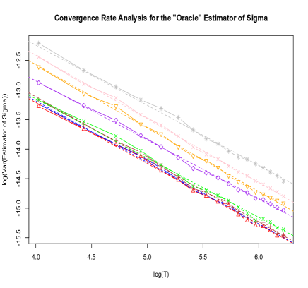
Figure 1: Regression Analysis of $\log(\widehat{{\rm Var}}\left(\hat{\bar{\sigma}}_{n,K^{*}_{2},T}\right)$ against $\log(T)$ (left panel) and $\log\left(\widehat{{\rm Var}}\left(\hat{\sigma}_{3}^{\prime\prime}\right)\right)$ (right panel) for $T\in\{2\text{ m},3\text{ m},\dots,24\text{ m}\}$, and $\delta_{n}=5\text{ sec}$ (Red), $\delta_{n}=10\text{ sec}$ (Blue), $\delta_{n}=30\text{ sec}$ (Brown), $\delta_{n}=1\text{ min}$ (Green), $\delta_{n}=10\text{ min}$ (Purple), $\delta_{n}=20\text{ min}$ (Orange), $\delta_{n}=30\text{ min}$ (Pink), and $\delta_{n}=1\text{ hr}$ (Grey). The sample variance is computed based on 200 simulations.

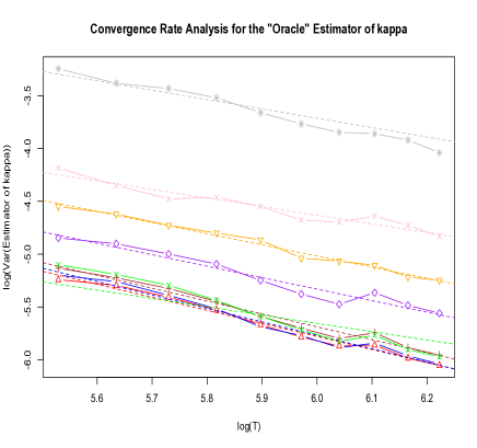
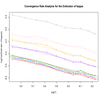
Figure 2: Regression Analysis of $\log(\widehat{{\rm Var}}\left(\hat{\bar{\kappa}}_{n,K^{*}_{2},T}\right)$ against $\log(T)$ (left panel) and $\log\left(\widehat{{\rm Var}}\left(\hat{\kappa}_{3}\right)\right)$ (right panel) for $T\in\{2\text{ m},3\text{ m},\dots,24\text{ m}\}$, and $\delta_{n}=5\text{ sec}$ (Red), $\delta_{n}=10\text{ sec}$ (Blue), $\delta_{n}=30\text{ sec}$ (Brown), $\delta_{n}=1\text{ min}$ (Green), $\delta_{n}=10\text{ min}$ (Purple), $\delta_{n}=20\text{ min}$ (Orange), $\delta_{n}=30\text{ min}$ (Pink), and $\delta_{n}=1\text{ hr}$ (Grey). The sample variance is computed based on 200 simulations.

5.4 Empirical study

We now proceed to analyze the performance of the proposed estimators when applied to real data. As it was explained above and was theoretically verified by Propositions 3.4-3.5, traditional estimators are not stable as the sampling frequency increases. Indeed, $\hat{\sigma}_{n}$ and $\tilde{\sigma}_{n}$ both diverge to $\infty$ while $\hat{\kappa}_{n}$ and $\tilde{\kappa}_{n}$ converge to $0$, as $n\to\infty$. The objective is to verify that the proposed estimators do not exhibit the aforementioned behaviors at very high-frequencies.

We consider high-frequency stock data for several stocks during 2005, which were obtained from the NYSE TAQ database of Wharton’s WRDS system. For briefness and illustration purposes, we only show Intel (INTC) and Pfeizer (PFE). For these, we compute the estimator $\hat{\varrho}$ defined in (5.1), the estimator $\hat{\sigma}_{n,K}$ defined in (4.1) with $K=1$, the estimator $\hat{\bar{\sigma}}_{n,K}$ defined in (4.7) with $K=\hat{\hat{K}}^{*}_{1}$ as given in (5.2), the estimator $\hat{\kappa}_{n,K}$ defined in (4.9) with $K=1$, and finally the estimator $\hat{\bar{\kappa}}_{n,K}$ defined in (4.13) with $K=\hat{K}_{4}^{*}$ as given in (4.28). In the case of $\hat{\kappa}_{n,1}$, we used $\sigma=\hat{\sigma}_{n,1}$. Both $\hat{\sigma}_{n,1}$ and $\hat{\kappa}_{n,1}$ represent the estimators without any technique to alleviate the effect of the microstructure noise. As one can see in Tables 5-6, the estimators $\hat{\bar{\sigma}}$ and $\hat{\bar{\kappa}}$ do not exhibit the drawbacks of the estimators $\hat{\sigma}$ and $\hat{\kappa}$ at high frequencies. As a conclusion of the empirical results therein, we deduce that Intel’s stock exhibits an annualized volatility $\sigma$ of about $0.014*\sqrt{252}=0.22$ per year, while its excess kurtosis increases with $1/\delta$ at a rate of about $0.5$ (see item 2 above Eq. (2.4) for the interpretation of $\kappa$). By comparison, even though the volatility of Pfizer’s stock is just slightly larger (about $0.015*\sqrt{252}=0.23$), its excess kurtosis increases at a rate of about $2.3$ with $1/\delta$, showing much more riskiness due to the much heavier tails of its return’s distribution. This example illustrates the importance of considering a parameter which measures the tail heaviness of the return distribution and not only its variance.

	$\hat{\varrho}$	$\hat{\sigma}_{n,1}$	$\hat{\bar{\sigma}}_{n,\hat{\hat{K}}^{*}_{1}}$	$\hat{\kappa}_{n,1}$	$\hat{\bar{\kappa}}_{n,\hat{K}^{*}_{4}}$
20 min	0.002198811	0.013732969	0.013115165	0.772846688	0.645084939
10 min	0.001584536	0.013995671	0.013112833	0.589344904	0.727208959
5 min	0.001152404	0.014394983	0.013253727	0.495378704	0.768302688
1 min	0.0005581856	0.0155908617	0.0136519981	0.3499494734	0.7293149570
30 sec	0.0004113675	0.0162494093	0.0139405766	0.2817929514	0.6875741045
20 sec	0.0003483541	0.0168528945	0.0141596310	0.2566280373	0.6575495762
10 sec	0.0002712869	0.0185608431	0.0145174963	0.1831341414	0.5921934015
5 sec	0.0002174315	0.0210381061	0.0147818871	0.1084570206	0.4987667343

Table 5: Estimation of the parameters $\sigma$ and $\kappa$ of a subordinated Brownian motion with microstructure noise for INTC (Intel) stock.

	$\hat{\varrho}$	$\hat{\sigma}_{n,1}$	$\hat{\bar{\sigma}}_{n,\hat{\hat{K}}^{*}_{1}}$	$\hat{\kappa}_{n,1}$	$\hat{\bar{\kappa}}_{n,\hat{K}^{*}_{4}}$
20 min	0.002310884	0.014432934	0.014279133	3.552809339	3.665645436
10 min	0.001678615	0.014826633	0.013921679	3.330420039	4.192632331
5 min	0.001223294	0.015280492	0.013758805	3.395593192	4.458814370
1 min	0.000581559	0.016243711	0.014289601	2.885849749	3.074717720
30 sec	0.0004379718	0.0173003060	0.0147847384	2.1009477905	2.5399891978
20 sec	0.0003733763	0.0180634325	0.0149589310	1.8189209947	2.3582752416
10 sec	0.0003021168	0.0206701623	0.0150440707	1.0395706194	2.3194219287
5 sec	0.0002547010	0.0246442060	0.0151395852	0.5255478783	2.3750789809

Table 6: Estimation of the parameters $\sigma$ and $\kappa$ of a subordinated Brownian motion with microstructure noise for PFE (Pfeizer) stock.

Appendix A Proofs

A.1 Proof of Proposition 3.2.

We shall need the following standard result that can easily be shown using the moment generating function for Poisson integrals (see, e.g., (Cont & Tankov, 2004, Chapter 2)):

Lemma A.1

Suppose that $M$ is a Poisson random measure on an open domain of ${\mathbb{R}}^{d}$ with mean measure $m$ and let $\bar{M}(f)=\int f(z)(M-m)(dz)$ denote the integral of $f$ with respect the compensated random measure $\bar{M}=M-m$. If $m(|f|^{k}):=\int|f(z)|^{k}m(dz)<\infty$, for $k=1,\dots,5$, then $\mathbb{E}\left(\bar{M}(f)^{k}\right)=m(f^{k})$, for $k=2,3$, $\mathbb{E}\left(\bar{M}(f)^{4}\right)=3m(f^{2})^{2}+m(f^{4})$, and $\mathbb{E}\left(\bar{M}(f)^{5}\right)=10m(f^{2})m(f^{3})+m(f^{5})$. Similarly, $\mathbb{E}\left(\bar{M}(g)\bar{M}(f)^{k}\right)=m(gf^{k})$ and $\mathbb{E}\left(\bar{M}(g)\bar{M}(f)^{3}\right)=m(gf^{3})+3m(f^{2})m(gf)$.

Lemma A.2

Let $M$ be the jump measure of a Lévy process $X$ with Lévy measure $\nu$ (i.e., $M((s,t)\times B):=\#\{u\in(s,t):\Delta X_{u}\in B\}$, for any $s<t$ and $B\in\mathcal{B}(\mathbb{R}^{d})$), and let $\bar{M}(dt,dx):=M(dt,dx)-dt\nu(dx)$ be the corresponding compensated measure. Also, suppose that $f$ is such that $\int|f(x)|^{k}\nu(dx)<\infty$ for some $k\geq{}2$. Then, there exists a constant $A_{k}(f)$ such that, for any $T\geq{}1$,

$$\mathbb{E}\left|\frac{1}{T}\int_{0}^{T}\int f(x)\bar{M}(dt,dx)\right|^{k}\leq A_{k}(f)T^{-k/2}.$$

Proof. Throughout the proof, let $\bar{M}_{s,t}(f):=\int_{s}^{t}\int f(x)\bar{M}(dt,dx)$ and let $[T]$ be the integer part of $T$. We need the following classical inequality (see (Bickel & Doksum, 2001, Lemma 5.3.1)):

$$\mathbb{E}|\bar{Z}_{n}-\mu_{Z}|^{k}\leq C_{k}\mathbb{E}|Z_{1}|^{k}n^{-k/2},$$ (A.1)

where $\bar{Z}_{n}=\frac{1}{n}\sum_{i=1}^{n}Z_{i}$, $\mu_{Z}=\mathbb{E}Z_{1}$, and $\{Z_{i}\}_{i}$ are i.i.d. such that $\mathbb{E}|Z_{1}|^{k}<\infty$. First, note that

$$\mathbb{E}\left|\frac{1}{T}\bar{M}_{0,T}(f)\right|^{k}\leq 2^{k}\mathbb{E}\left|\frac{[T]}{T}\frac{1}{[T]}\bar{M}_{0,[T]}\left(f\right)\right|+2^{k}\frac{1}{T^{k}}\mathbb{E}\left|\bar{M}_{[T],T}(f)\right|^{k}.$$

For the first term on the right-hand side above, we apply (A.1) with $Z_{i}:=\bar{M}_{i-1,i}(f)$, which are i.i.d. because $M$ is a Poisson random measure. For the second term, we apply Burkholder-Davis-Gundy inequality (see Protter (2004)) to get,

$$\mathbb{E}\left|\int_{[T]}^{T}\int f(x)\bar{M}(dt,dx)\right|^{k}\leq B_{k}^{k}\mathbb{E}\left|\int_{0}^{1}\int f^{2}(x)M(dt,dx)\right|^{k/2}.$$

This completes the proof. $\Box$

Proof of Proposition 3.2. Throughout the proof, $M$ denotes the jump measure of the Lévy process $X$; i.e., $M((s,t)\times B):=\#\{u\in(s,t):\Delta X_{u}\in B\}$, for any $s<t$ and $B\in\mathcal{B}(\mathbb{R})$. In particular, let us note that $M$ is Poisson random measure with mean measure $dt\nu(dx)$ and $\sum_{t\leq{}T}(\Delta X_{t})^{\ell}=\int_{0}^{t}\int x^{\ell}M(dt,dx)$. Let also $\bar{M}(dt,dx):=M(dt,dx)-dt\nu(dx)$ be the corresponding compensated measure. Let us start by noting the identity

$$\frac{1}{(1+x)^{2}}=\sum_{i=0}^{k-1}(-1)^{i}(i+1)x^{i}+\frac{(-1)^{k}x^{k}}{(1+x)^{2}}(k+1+kx),$$ (A.2)

and the notation

$$\hat{\mu}_{k}^{(T)}:=\frac{1}{T}\int_{0}^{T}\int x^{k}M(dt,dx),\quad\hat{D}_{T}:=\frac{\hat{\mu}_{2}^{(T)}}{c_{2}(X_{1})}-1.$$

In particular, $\hat{\kappa}^{(T)}=(1/3)\hat{\mu}_{4}^{(T)}/(\hat{\mu}_{2}^{(T)})^{2}$. Then, we have the following decomposition:

$$\mathbb{E}\hat{\kappa}^{(T)} =\frac{1}{3c_{2}^{2}(X_{1})}\mathbb{E}\left\{\frac{\hat{\mu}_{4}^{(T)}}{(1+\hat{D}_{T})^{2}}\right\}$$

$$=\frac{1}{3c_{2}^{2}(X_{1})}\mathbb{E}\left\{\hat{\mu}_{4}^{(T)}\left(1-2\hat{D}_{T}+3\hat{D}_{T}^{2}-4\hat{D}_{T}^{3}+5\hat{D}_{T}^{4}-6\hat{D}_{T}^{5}\right)\right\}$$

$$\quad+\frac{1}{3}\mathbb{E}\left\{\hat{\mu}_{4}^{(T)}\left(\hat{\mu}_{2}^{(T)}\right)^{-2}\left(7+6\hat{D}_{T}\right)\hat{D}_{T}^{6}\right\}$$

$$=:L_{T}+R_{T}.$$

Let us first analyze the residual term $R_{T}$ using the following easy consequence of the triangle inequality:

$$(\hat{\mu}_{4}^{(T)})^{1/2}=\frac{1}{T^{1/2}}\left(\sum_{s\leq{}T}\left(\Delta X_{s}\right)^{4}\right)^{1/2}\leq\frac{1}{T^{1/2}}\sum_{s\leq{}T}\left(\Delta X_{s}\right)^{2}=T^{1/2}\mu_{2}^{(T)}.$$ (A.3)

Thus, since $7+6\hat{D}_{T}=1+6(1+\hat{D}_{T})=1+6\hat{\mu}_{2}^{(T)}/c_{2}(X_{1})>0$, we have that

$$0\leq R_{T} \leq\frac{7T}{3}\mathbb{E}\left(\hat{D}_{T}^{6}\right)+\frac{6T}{3}\mathbb{E}\left(\hat{D}_{T}^{7}\right)$$

$$=\frac{7T}{3c_{2}^{6}(X_{1})}\mathbb{E}\left(\hat{\mu}_{2}^{(T)}-c_{2}(X_{1})\right)^{6}+\frac{6T}{3c_{2}^{7}(X_{1})}\mathbb{E}\left(\hat{\mu}_{2}^{(T)}-c_{2}(X_{1})\right)^{7}.$$

Using that $\mathbb{E}\hat{\mu}_{2}^{(T)}=c_{2}(X_{1})$ and Lemma A.2, $R_{T}=O(T^{-2}).$ Similarly, using Lemma A.1, the first four terms of $L_{T}$ (i.e. those multiplying $\hat{D}^{i}_{T}$ up to $i=3$) are given by

$$\frac{c_{4}(X_{1})}{3c_{2}^{2}(X_{1})}-\frac{2c_{6}(X_{1})}{3c_{2}^{3}(X_{1})}T^{-1}+\frac{c_{4}^{2}(X_{1})}{c_{2}^{4}(X_{1})}T^{-1}+O(T^{-2}).$$

The last two term of $L_{T}$ can be seen to be $O(T^{-2})$ from Lemma A.2 and Cauchy inequality. Indeed,

$$\left|\mathbb{E}\hat{\mu}_{4}^{(T)}\hat{D}_{T}^{4}\right| \leq c_{4}(X_{1})\left|\mathbb{E}\hat{D}_{T}^{4}\right|+\frac{1}{c_{2}^{4}(X_{1})}\left|\mathbb{E}\left(\hat{\mu}_{4}^{(T)}-c_{4}(X_{1})\right)\left(\hat{\mu}_{2}^{(T)}-c_{2}(X_{1})\right)^{4}\right|$$

$$\leq Kc_{2}T^{-2}+\left(\mathbb{E}\left(\hat{\mu}_{4}^{(T)}-c_{4}(X_{1})\right)^{2}\mathbb{E}\left(\hat{\mu}_{2}^{(T)}-c_{2}(X_{1})\right)^{8}\right)^{1/2},$$

which is $O(T^{-2})$ in light of Lemma A.2. We finally obtain that

$$\mathbb{E}\hat{\kappa}_{n}{\;{\stackrel{{\scriptstyle n\to\infty}}{{\longrightarrow}}}\;}\mathbb{E}\hat{\kappa}^{(T)}=\frac{c_{4}(X_{1})}{3c_{2}^{2}(X_{1})}-\frac{2c_{6}(X_{1})}{3c_{2}^{3}(X_{1})}T^{-1}+\frac{c_{4}^{2}(X_{1})}{c_{2}^{4}(X_{1})}T^{-1}+O(T^{-2}).$$

In order to show the bound for the variance, we use again (A.2) to get

$$\hat{\kappa}^{(T)} =\frac{\hat{\mu}_{4}^{(T)}}{3c_{2}^{2}(X_{1})}\left(1-2\hat{D}_{T}+3\hat{D}_{T}^{2}-4\hat{D}_{T}^{3}\right)+\frac{1}{3}\frac{\hat{\mu}_{4}^{(T)}}{\left(\hat{\mu}_{2}^{(T)}\right)^{2}}\left(5+4\hat{D}_{T}\right)\hat{D}_{T}^{4}.$$

Then,

$$\hat{\kappa}^{(T)}-\frac{c_{4}(X_{1})}{3c_{2}^{2}(X_{1})} =\frac{1}{3c_{2}^{2}(X_{1})}\left(\hat{\mu}_{4}^{(T)}-c_{4}(X_{1})\right)-\frac{2\hat{\mu}_{4}^{(T)}}{3c_{2}^{2}(X_{1})}\hat{D}_{T}+\frac{\hat{\mu}_{4}^{(T)}}{c_{2}^{2}(X_{1})}\hat{D}_{T}^{2}$$

$$\quad-\frac{4\hat{\mu}_{4}^{(T)}}{3c_{2}^{2}(X_{1})}\hat{D}_{T}^{3}+\frac{1}{3}\frac{\hat{\mu}_{4}^{(T)}}{\left(\hat{\mu}_{2}^{(T)}\right)^{2}}\left(5+4\hat{D}_{T}\right)\hat{D}_{T}^{4}.$$

After expanding the squares, taking expectations both sides, and using Cauchy’s inequality together with Lemmas A.1 and A.2, one can check that all the terms are at least $O(T^{-2})$ except possibly the following terms:

$$\frac{1}{9c_{2}^{4}(X_{1})}\mathbb{E}\left\{\left(\hat{\mu}_{4}^{(T)}-c_{4}(X_{1})\right)^{2}\right\}-\frac{4}{9c_{2}^{4}(X_{1})}\mathbb{E}\left\{\left(\hat{\mu}_{4}^{(T)}-c_{4}(X_{1})\right)\hat{\mu}_{4}^{(T)}\hat{D}_{T}\right\}$$

$$+\frac{4}{9c_{2}^{4}(X_{1})}\mathbb{E}\left\{(\hat{\mu}_{4}^{(T)})^{2}\hat{D}_{T}^{2}\right\}.$$

Subtracting $c_{4}(X_{1})$ from $\hat{\mu}_{4}^{(T)}$ in the second and third terms above, and using again Lemmas A.1 and A.2, we can check that the above expression indeed coincides with the expression in (3.9). $\Box$

A.2 Proofs of Section 4.

Proof of Theorem 4.3. Throughout we write $T_{i}$ for $T_{i,K}$. Clearly,

$${\rm Var}\left(\hat{\sigma}^{2}_{n,K}\right)=\frac{2}{K^{2}}\sum_{1\leq i<j\leq K}\frac{1}{{T_{i}T_{j}}}{\rm Cov}\left([\widetilde{X},\widetilde{X}]_{2}^{\mathcal{G}_{n}^{(i)}},[\widetilde{X},\widetilde{X}]_{2}^{\mathcal{G}_{n}^{(j)}}\right)+\frac{1}{K^{2}}\sum_{i=1}^{K}\frac{1}{{T_{i}^{2}}}{\rm Var}\left([\widetilde{X},\widetilde{X}]_{2}^{\mathcal{G}_{n}^{(i)}}\right).$$ (A.4)

Each covariance in the first term on the right hand side above is given by

$$A_{i,j} :={\rm Cov}\left([\widetilde{X},\widetilde{X}]_{2}^{\mathcal{G}_{n}^{(i)}},[\widetilde{X},\widetilde{X}]_{2}^{\mathcal{G}_{n}^{(j)}}\right)$$

$$=\sum_{q=0}^{n_{i}-1}\sum_{r=0}^{n_{j}-1}{\rm Cov}\left(\left|\widetilde{X}(t_{i-1+(q+1)K})-\widetilde{X}(t_{i-1+qK})\right|^{2},\left|\widetilde{X}(t_{j-1+(r+1)K})-\widetilde{X}(t_{j-1+rK})\right|^{2}\right)$$

$$=n_{i}C\left((K+i-j)\delta_{n}\right)+\left(n_{j}-1\right)C\left((j-i)\delta_{n}\right),$$

where, for any $u<t<t+\delta<v$, $C(\delta):={\rm Cov}\left(\left|\widetilde{X}(t+\delta)-\widetilde{X}(u)\right|^{2},\left|\widetilde{X}(v)-\widetilde{X}(t)\right|^{2}\right),$ which can be proved to depend only on $\delta>0$. More specifically, note that $C(\delta)={\rm Cov}\left(\left|S+U\right|^{2},\left|S+V\right|^{2}\right)$, where $S:=X(t+\delta)-{X}(t)$, $U:={X}(t)-{X}(u)+\varepsilon_{t+\delta}-\varepsilon_{u}$, and $V:={X}(v)-{X}(t+\delta)+\varepsilon_{v}-\varepsilon_{t}$. Next, using that independence of $S$, $U$, and $V$,

$$C(\delta) ={\rm Var}\left(S^{2}\right)+2{\rm Cov}\left(S^{2},SV\right)+2{\rm Cov}\left(SU,S^{2}\right)+4{\rm Cov}\left(SU,SV\right)$$

$$={\rm Var}\left(S^{2}\right)+2\mathbb{E}(V){\rm Cov}\left(S^{2},S\right)+2\mathbb{E}(U){\rm Cov}\left(S,S^{2}\right)+4\mathbb{E}(U)\mathbb{E}(V){\rm Var}\left(S\right).$$

Finally, using that $\mathbb{E}U=\mathbb{E}V=0$ as well as the moment formulas in (3.1), $C(\delta)={\rm Var}\left(S^{2}\right)$ is given by $C(\delta)=2\sigma^{4}\delta^{2}+3\sigma^{4}\kappa\delta$. Using the previous formula together with the fact that $|\frac{n(n_{j}-1)}{Kn_{i}n_{j}}-1|\leq{}U\frac{K}{n}$ and $|\frac{n}{Kn_{j}}-1|\leq{}U\frac{K}{n}$ for some constant $U$ (independent of $n$, $K$, $i$, $T$, and $j$), the first term in (A.4), which we denote $A$, can be computed as follows:

$$A ={\frac{2n}{K^{3}T^{2}}}\sum_{1\leq i<j\leq K}\left(2\sigma^{4}(j-i)^{2}\delta_{n}^{2}+3\sigma^{4}\kappa(j-i)\delta_{n}\right)$$

$$\quad+{\frac{2n}{K^{3}T^{2}}}\sum_{1\leq i<j\leq K}\left(2\sigma^{4}(K+i-j)^{2}\delta_{n}^{2}+3\sigma^{4}\kappa(K+i-j)\delta_{n}\right)+\mathcal{R}$$

$$=\frac{n}{K}\frac{K-1}{KT^{2}}\left({3\sigma^{4}\kappa K\delta_{n}+\frac{2}{3}\sigma^{4}K(2K-1)\delta_{n}^{2}}\right)+\mathcal{R}_{1},$$

where $\mathcal{R}$ is such that

$$|\mathcal{R}_{1}| \leq\frac{{2U}(K-1)}{KT^{2}}\left({3\sigma^{4}\kappa K\delta_{n}+\frac{2}{3}\sigma^{4}K(2K-1)\delta_{n}^{2}}\right).$$ (A.5)

Now, we consider the second term in (A.4), which we denote $B$. Each variance term of $B$ can be written as

$$B_{i} :={\rm Var}\left([\widetilde{X},\widetilde{X}]_{2}^{\mathcal{G}_{n}^{(i)}}\right)$$

$$=\sum_{q=0}^{n_{i}-1}{\rm Var}\left(\left|\widetilde{X}(t_{i-1+(q+1)K})-\widetilde{X}(t_{i-1+qK})\right|^{2}\right)$$

$$\quad+2\sum_{q=0}^{n_{i}-2}{\rm Cov}\left(\left|\widetilde{X}(t_{i-1+(q+1)K})-\widetilde{X}(t_{i-1+qK})\right|^{2},\left|\widetilde{X}(t_{i-1+(q+2)K})-\widetilde{X}(t_{i-1+(q+1)K})\right|^{2}\right).$$

Next, using the relationships

$${\rm Var}\left(\left|\widetilde{X}(t+\delta)-\widetilde{X}(t)\right|^{2}\right)=2\sigma^{4}\delta^{2}+3\sigma^{4}\kappa\delta+8\sigma^{2}\mathbb{E}\left(\varepsilon^{2}\right)\delta+2\mathbb{E}\left(\varepsilon^{2}\right)^{2}+2\mathbb{E}\left(\varepsilon^{4}\right)$$

$${\rm Cov}\left(\left|\widetilde{X}(t+\delta)-\widetilde{X}(t)\right|^{2},\left|\widetilde{X}(v)-\widetilde{X}(t+\delta)\right|^{2}\right)=\mathbb{E}\left(\varepsilon^{4}\right)-\mathbb{E}\left(\varepsilon^{2}\right)^{2},$$

valid for any $t<t+\delta<v$, we get

$$B_{i} =n_{i}\left(2\sigma^{4}\left(K\delta_{n}\right)^{2}+3\sigma^{4}\kappa\left(K\delta_{n}\right)+8\sigma^{2}\mathbb{E}\left(\varepsilon^{2}\right)\left(K\delta_{n}\right)\right)+2(2n_{i}-1)\mathbb{E}\left(\varepsilon^{4}\right)+2\mathbb{E}\left(\varepsilon^{2}\right)^{2}.$$ (A.6)

Therefore, using that $|1/n_{i}-K/n|\leq{}UK^{2}/n^{2}$ and $|1/n^{2}_{i}-K^{2}/n^{2}|\leq{}UK^{3}/n^{3}$, for a constant $U$ independent of $i$, $K$, $n$, and $T$, we have $B=C_{1}-C_{2}+\mathcal{R}_{2},$ where

$$C_{1} =\frac{n}{K^{2}T^{2}}\left(2\sigma^{4}\left(K\delta_{n}\right)^{2}+3\sigma^{4}\kappa\left(K\delta_{n}\right)+8\sigma^{2}\mathbb{E}\left(\varepsilon^{2}\right)\left(K\delta_{n}\right)+4\mathbb{E}\left(\varepsilon^{4}\right)\right),$$

$$C_{2} =\frac{2}{KT^{2}}\left(\mathbb{E}\left(\varepsilon^{4}\right)-\mathbb{E}\left(\varepsilon^{2}\right)^{2}\right),$$

and $\mathcal{R}_{2}=O_{u}\left((K/n)C_{1}\right)=O_{u}\left((K/n)C_{2}\right)$. Putting together $A$ and $B$ above,

$${\rm Var}\left(\hat{\sigma}^{2}_{n,K}\right) =\frac{n}{K}\frac{K-1}{KT^{2}}\left({3\sigma^{4}\kappa K\delta_{n}+\frac{2}{3}\sigma^{4}K(2K-1)\delta_{n}^{2}}\right)$$

$$\quad+\frac{n}{K^{2}T^{2}}\left(2\sigma^{4}\left(K\delta_{n}\right)^{2}+3\sigma^{4}\kappa\left(K\delta_{n}\right)+8\sigma^{2}\mathbb{E}\left(\varepsilon^{2}\right)\left(K\delta_{n}\right)+4\mathbb{E}\left(\varepsilon^{4}\right)\right)$$

$$\quad-\frac{2}{KT^{2}}\left(\mathbb{E}\left(\varepsilon^{4}\right)-\mathbb{E}\left(\varepsilon^{2}\right)^{2}\right)+\mathcal{R}_{1}+\mathcal{R}_{2}.$$ (A.7)

Recalling that $\delta_{n}=T/n$ and using (A.5), we get the expression (4.14). $\Box$

Proof of Proposition 4.5. Let $a_{K}:=\frac{K}{K-1}$ and $b_{K}:=\frac{1}{T(K-1)}$. Clearly,

$${\rm Var}\left(\hat{\bar{\sigma}}^{2}_{n,K}\right) =a_{K}^{2}{\rm Var}\left(\hat{\sigma}^{2}_{n,K}\right)+b_{K}^{2}{\rm Var}\left([\widetilde{X},\widetilde{X}]_{2}^{\bar{\mathcal{G}}_{n}}\right)-2a_{K}b_{K}{\rm Cov}\left(\hat{\sigma}^{2}_{n,K},[\widetilde{X},\widetilde{X}]_{2}^{\bar{\mathcal{G}}_{n}}\right)$$

From the expressions in Eqs. (A.6)-(A.7), we have

$${\rm Var}\left([\widetilde{X},\widetilde{X}]_{2}^{\bar{\mathcal{G}}_{n}}\right) =n\left(2\sigma^{4}\delta_{n}^{2}+3\sigma^{4}\kappa\delta_{n}+8\sigma^{2}\mathbb{E}\left(\varepsilon^{2}\right)\delta_{n}\right)+2(2n-1)\mathbb{E}\left(\varepsilon^{4}\right)+2\mathbb{E}\left(\varepsilon^{2}\right)^{2}$$

$${\rm Var}\left(\hat{\sigma}^{2}_{n,K}\right) =\frac{n}{K}\frac{K-1}{KT^{2}}\left({3\sigma^{4}\kappa K\delta_{n}+\frac{2}{3}\sigma^{4}K(2K-1)\delta_{n}^{2}}\right)$$

$$\quad+\frac{n-K+1}{K^{2}T^{2}}\left(2\sigma^{4}\left(K\delta_{n}\right)^{2}+3\sigma^{4}\kappa\left(K\delta_{n}\right)+8\sigma^{2}\mathbb{E}\left(\varepsilon^{2}\right)\left(K\delta_{n}\right)+4\mathbb{E}\left(\varepsilon^{4}\right)\right)$$

$$\quad-\frac{2}{KT^{2}}\left(\mathbb{E}\left(\varepsilon^{4}\right)-\mathbb{E}\left(\varepsilon^{2}\right)^{2}\right)+\mathcal{R}_{1}+\mathcal{R}_{2}.$$

To compute the last covariance, let us first note that

$${\rm Cov}\left(\hat{\sigma}^{2}_{n,K},[\widetilde{X},\widetilde{X}]_{2}^{\bar{\mathcal{G}}_{n}}\right)=\frac{1}{K}\sum_{i=1}^{K}{\frac{1}{T_{i}}}{\rm Cov}\left([\widetilde{X},\widetilde{X}]_{2}^{\mathcal{G}_{n}^{(i)}},[\widetilde{X},\widetilde{X}]_{2}^{\bar{\mathcal{G}}_{n}}\right)=:\frac{1}{K}\sum_{i=1}^{K}{\frac{1}{T_{i}}}B_{i}.$$ (A.8)

Each covariance term on the right hand side above can be computed as

$$B_{i} =\sum_{q=0}^{n_{i}-1}\sum_{r=0}^{n-1}{\rm Cov}\left(\left|\widetilde{X}(t_{i-1+(q+1)K})-\widetilde{X}(t_{i-1+qK})\right|^{2},\left|\widetilde{X}(t_{r+1})-\widetilde{X}(t_{r})\right|^{2}\right)$$

$$=(n_{i}-e_{i})\sum_{r=0}^{n-1}{\rm Cov}\left(\left|\widetilde{X}(t_{i-1+2K})-\widetilde{X}(t_{i-1+K})\right|^{2},\left|\widetilde{X}(t_{r+1})-\widetilde{X}(t_{r})\right|^{2}\right)$$

$$\quad+e_{i}\sum_{r=0}^{n-1}{\rm Cov}\left(\left|\widetilde{X}(t_{K})-\widetilde{X}(t_{0})\right|^{2},\left|\widetilde{X}(t_{r+1})-\widetilde{X}(t_{r})\right|^{2}\right),$$

where above $e_{i}$ denote the number of subintervals in the set $\left\{[t_{i-1+qK},t_{i-1+(q+1)K}]\right\}_{{q=0}}^{{n_{i}-1}}$ which intersect the end points $0$ and $T$. Obviously, $\sum_{i=1}^{K}e_{i}=2$. Now, we use the following formulas:

$${\rm Cov}\left(|\widetilde{X}(v)-\widetilde{X}(u)|^{2},|\widetilde{X}(v^{\prime})-\widetilde{X}(u^{\prime})|^{2}\right)={2\sigma^{4}(v^{\prime}-u^{\prime})^{2}+3\kappa\sigma^{4}(v^{\prime}-u^{\prime})},\quad u<u^{\prime}<v^{\prime}<v$$

$${\rm Cov}\left(|\widetilde{X}(t)-\widetilde{X}(s)|^{2},|\widetilde{X}(u)-\widetilde{X}(t)|^{2}\right)=\mathbb{E}\varepsilon^{4}-(\mathbb{E}\varepsilon^{2})^{2},\qquad s<t<u.$$

We then get $B_{i}=n_{i}\left\{K\left({2\sigma^{4}\delta_{n}^{2}+3\kappa\sigma^{4}\delta_{n}}\right)+2(\mathbb{E}\varepsilon^{4}-(\mathbb{E}\varepsilon^{2})^{2})\right\}-e_{i}(\mathbb{E}\varepsilon^{4}-(\mathbb{E}\varepsilon^{2})^{2}).$ Next,

$${\rm Cov}\left(\hat{\sigma}^{2}_{n,K},[\widetilde{X},\widetilde{X}]_{2}^{\bar{\mathcal{G}}_{n}}\right) =\frac{n}{KT}\left\{K\left({2\sigma^{4}\delta_{n}^{2}+3\kappa\sigma^{4}\delta_{n}}\right)+2(\mathbb{E}\varepsilon^{4}-(\mathbb{E}\varepsilon^{2})^{2})\right\}+O_{u}\left(\frac{1}{KT}\right)$$

Putting together the previous relationships,

$${\rm Var}\left(\hat{\bar{\sigma}}^{2}_{n,K}\right) =a_{K}^{2}{\rm Var}\left(\hat{\sigma}^{2}_{n,K}\right)+b_{K}^{2}{\rm Var}\left([\widetilde{X},\widetilde{X}]_{2}^{\bar{\mathcal{G}}_{n}}\right)-2a_{K}b_{K}{\rm Cov}\left(\hat{\sigma}^{2}_{n,K},[\widetilde{X},\widetilde{X}]_{2}^{\bar{\mathcal{G}}_{n}}\right)$$

$$=\left(\frac{4\sigma^{4}K}{3n}+4\frac{n}{K^{2}T^{2}}\mathbb{E}(\varepsilon^{4})\right)+O_{u}\left(\frac{1}{n}\right)+O_{u}\left(\frac{n}{K^{3}T^{2}}\right)$$

$$\quad+\frac{1}{T^{2}K^{2}}\left(4n\mathbb{E}\varepsilon^{4}\right)-\frac{4n}{T^{2}K^{2}}(\mathbb{E}\varepsilon^{4}-(\mathbb{E}\varepsilon^{2})^{2})+O_{u}\left(\frac{1}{TK}\right)$$

$$={\frac{4\sigma^{4}K}{3n}+\frac{4n\left(\mathbb{E}\left(\varepsilon^{4}\right)+(\mathbb{E}\varepsilon^{2})^{2}\right)}{T^{2}K^{2}}+O_{u}\left(\frac{1}{n}\right)+O_{u}\left(\frac{n}{K^{3}T^{2}}\right)+O_{u}\left(\frac{1}{TK}\right).}$$

$\Box$

Proof of Theorem 4.6. Let us first write the variance of the estimator as follows:

$${\rm Var}\left(\hat{\kappa}_{n,K}\right) =\frac{2}{9\sigma^{8}K^{2}}\sum_{1\leq i<j\leq K}\frac{1}{T_{i}T_{j}}{\rm Cov}\left([\widetilde{X},\widetilde{X}]_{4}^{\mathcal{G}_{n}^{(i)}},[\widetilde{X},\widetilde{X}]_{4}^{\mathcal{G}_{n}^{(j)}}\right)+\frac{1}{9\sigma^{8}K^{2}}\sum_{i=1}^{K}\frac{1}{T_{i}^{2}}{\rm Var}\left([\widetilde{X},\widetilde{X}]_{4}^{\mathcal{G}_{n}^{(i)}}\right)$$

$$=:A+B.$$ (A.9)

Let us first note that we can replace $1/(T_{i}T_{j})=1/(K^{2}\delta_{n}^{2}n_{i}n_{j})$ with $1/T^{2}$ for any $1\leq{}i\leq{}j\leq{}K$, since $|1/(n_{i}n_{j})-K^{2}/n^{2}|\leq{}UK^{3}/n^{3}$, for a constant $U$ independent of $i,j,K,n,T$, and, thus,

$$\left|\frac{1}{T_{i}T_{j}}-\frac{1}{T^{2}}\right|\leq{}U\frac{K}{T^{2}n}.$$ (A.10)

Next, each covariance in the first term of (A.2) can be computed as:

$$A_{i,j} :={\rm Cov}\left([\widetilde{X},\widetilde{X}]_{4}^{\mathcal{G}_{n}^{(i)}},[\widetilde{X},\widetilde{X}]_{4}^{\mathcal{G}_{n}^{(j)}}\right)$$

$$=\sum_{q=0}^{n_{i}-1}\sum_{r=0}^{n_{j}-1}{\rm Cov}\left(\left|\widetilde{X}(t_{i-1+(q+1)K})-\widetilde{X}(t_{i-1+qK})\right|^{4},\left|\widetilde{X}(t_{j-1+(r+1)K})-\widetilde{X}(t_{j-1+rK})\right|^{4}\right)$$

$$=n_{i}{\rm Cov}\left(\left|\widetilde{X}(t_{i-1+K})-\widetilde{X}(t_{i-1})\right|^{4},\left|\widetilde{X}(t_{j-1+K})-\widetilde{X}(t_{j-1})\right|^{4}\right)$$

$$\quad+(n_{j}-1){\rm Cov}\left(\left|\widetilde{X}(t_{i-1+2K})-\widetilde{X}(t_{i-1+K})\right|^{4},\left|\widetilde{X}(t_{j-1+K})-\widetilde{X}(t_{j-1})\right|^{4}\right)$$

$$=n_{i}C\left((j-i)\delta_{n},(K+i-j)\delta_{n},(j-i)\delta_{n}\right)$$

$$\quad+\left(n_{j}-1\right)C\left((K+i-j)\delta_{n},(j-i)\delta_{n},(K+i-j)\delta_{n}\right),$$

where, for any $t,{s}_{1},{s}_{2},{s}_{3}>0$,

$$C({s}_{1},{s}_{2},{s}_{3}):={\rm Cov}\left(\left|\widetilde{X}_{t+{s}_{1}+{s}_{2}}-\widetilde{X}_{t}\right|^{4},\left|\widetilde{X}_{t+{s}_{1}+{s}_{2}+{s}_{3}}-\widetilde{X}_{t+{s}_{1}}\right|^{4}\right),$$ (A.11)

which again can be proved to be independent of $t$. Concretely, with the notation $S:=X_{t+s_{1}+s_{2}}-X_{t+s_{1}}$, $U:=X_{t+s_{1}}-X_{t}+\varepsilon_{t+s_{1}+s_{2}}-\varepsilon_{t}$, and $V:=X_{t+s_{1}+s_{2}+s_{3}}-X_{t+s_{1}+s_{2}}+\varepsilon_{t+s_{1}+s_{2}+s_{3}}-\varepsilon_{t+s_{1}}$

$$C(s_{1},s_{2},s_{3}) ={\rm Cov}\left(\left|S+U\right|^{4},\left|S+V\right|^{4}\right)$$

$$={\rm Var}\left(S^{4}\right)+6\left[\mathbb{E}(U^{2})+\mathbb{E}(V^{2})\right]{\rm Cov}\left(S^{4},S^{2}\right)$$

$$\quad+36\mathbb{E}(U^{2})\mathbb{E}(V^{2}){\rm Var}\left(S^{2}\right)+16\mathbb{E}(U^{3})\mathbb{E}(V^{3}){\rm Var}\left(S\right)$$

where above we used the independence of $S$, $U$, and $V$ as well as the fact that $\mathbb{E}U=\mathbb{E}V=\mathbb{E}S^{k}=0$ for any odd positive integer $k$. Upon computation of the relevant moments of $U$ and $V$, we get

$$C(s_{1},s_{2},s_{3}) ={\rm Var}\left(X_{s_{2}}^{4}\right)+6\left[\sigma^{2}(s_{1}+s_{3})+4\mathbb{E}\varepsilon^{2}\right]{\rm Cov}\left(X_{s_{2}}^{4},X_{s_{2}}^{2}\right)$$

$$\quad+6^{2}\left(\sigma^{2}s_{1}+2\mathbb{E}\varepsilon\right)\left(\sigma^{2}s_{3}+2\mathbb{E}\varepsilon\right){\rm Var}\left(X_{s_{2}}^{2}\right)+4^{2}\left(2\mathbb{E}\varepsilon^{3}\right)^{2}{\rm Var}\left(X_{s_{2}}\right).$$ (A.12)

Note that

$$\mathbb{E}X_{s}^{k}=\mathbb{E}\left({(\sigma W_{\tau_{s}})}^{k}\right)=\sigma^{k}\mathbb{E}\left(W_{1}^{k}\right)\mathbb{E}\left(\tau_{s}^{k/2}\right)=\sigma^{k}\mathbb{E}\left(W_{1}^{k}\right)\left(s^{k/2}+\sum_{i=1}^{k/2-1}a_{k,i}s^{i}\right),$$

for some constant $a_{k,i}$’s. We now proceed to analyze each term separately:

• The contribution to $A$ due to ${\rm Var}\left(X_{s_{2}}^{4}\right)$ can be written as:

  $$A^{(1)} :=\frac{n}{K}\frac{2}{9\sigma^{8}K^{2}}\sum_{1\leq i<j\leq K}{\frac{1}{T_{i}T_{j}}}{\rm Var}\left({X}_{(K+i-j)\delta_{n}}^{4}\right)+\frac{n}{K}\frac{2}{9\sigma^{8}K^{2}}\sum_{1\leq i<j\leq K}{\frac{1}{T_{i}T_{j}}}{\rm Var}\left({X}_{(j-i)\delta_{n}}^{4}\right).$$

  Using (A.10) and that ${\rm Var}\left(X_{t}^{4}\right)$ is a polynomial of degree $4$ in $t$ with the highest-degree term being $96\sigma^{8}t^{4}$,

  $$A^{(1)} =\frac{n}{K}\frac{192\delta_{n}^{4}}{9K^{2}T^{2}}\left(\sum_{1\leq i<j\leq K}(K+i-j)^{4}+\sum_{1\leq i<j\leq K}(j-i)^{4}+O\left(K^{5}\right)\right)$$

  $$=\frac{192}{5(9)}\frac{T^{2}K^{3}}{n^{3}}+O\left(\frac{T^{2}K^{2}}{n^{3}}\right).$$

• Let us analyze the contribution to $A$ due to ${\rm Var}\left(X_{s_{2}}^{2}\right)$. Using again (A.10) and the variance formula in (3.1), the leading term is given by:

  $$A^{(2)} :=6^{2}\frac{n}{K}\frac{2}{9\sigma^{8}K^{2}}\sum_{1\leq i<j\leq K}\frac{1}{T_{i}T_{j}}\left(\sigma^{2}(j-i)\delta_{n}\right)^{2}{\rm Var}\left({X}_{(K+i-j)\delta_{n}}^{2}\right)$$

  $$\quad+6^{2}\frac{n}{K}\frac{2}{9\sigma^{8}K^{2}T^{2}}\sum_{1\leq i<j\leq K}\left(\sigma^{2}(K+i-j)\delta_{n}\right)^{2}{\rm Var}\left({X}_{(j-i)\delta_{n}}^{2}\right)$$

  $$=6^{2}\frac{n}{K}\frac{2}{9\sigma^{8}K^{2}T^{2}}\sum_{1\leq i<j\leq K}\left(\sigma^{2}(j-i)\delta_{n}\right)^{2}\left(3\sigma^{4}\kappa(K+i-j)\delta_{n}+2\sigma^{4}(K+i-j)^{2}\delta_{n}^{2}\right)$$

  $$\quad+6^{2}\frac{n}{K}\frac{2}{9\sigma^{8}K^{2}T^{2}}\sum_{1\leq i<j\leq K}\left(\sigma^{2}(K+i-j)\delta_{n}\right)^{2}\left(3\sigma^{4}\kappa(j-i)\delta_{n}+2\sigma^{4}(j-i)^{2}\delta_{n}^{2}\right)$$

  $$=\frac{(6)(4)(13)}{5(9)}\frac{T^{2}K^{3}}{n^{3}}+O\left(\frac{T^{2}K^{2}}{n^{3}}\right)$$

• The contribution to $A$ due to ${\rm Cov}\left(X_{s_{2}}^{4},X_{s_{2}}^{2}\right)$ has the following leading term:

  $$A^{(3)} :=6\frac{n}{K}\frac{2}{9\sigma^{8}K^{2}T^{2}}\sum_{1\leq i<j\leq K}\left(2\sigma^{2}(j-i)\delta_{n}\right){\rm Cov}\left({X}_{(K+i-j)\delta_{n}}^{2},{X}_{(K+i-j)\delta_{n}}^{4}\right)$$

  $$\quad+6\frac{n}{K}\frac{2}{9\sigma^{8}K^{2}T^{2}}\sum_{1\leq i<j\leq K}\left(2\sigma^{2}(K+i-j)\delta_{n}\right){\rm Cov}\left({X}_{(j-i)\delta_{n}}^{2},{X}_{(j-i)\delta_{n}}^{4}\right)$$

  $$=\frac{12^{2}(2)}{(5)(4)(9)}\frac{T^{2}K^{3}}{n^{3}}+O\left(\frac{T^{2}K^{2}}{n^{3}}\right)$$

  where above we used that ${\rm Cov}\left(X_{s}^{2},X_{s}^{4}\right)=\mathbb{E}X_{s}^{6}-\mathbb{E}(X_{s}^{2})\mathbb{E}(X_{s}^{4})=12\sigma^{6}s^{3}+{\text{h.o.t.}}$, where h.o.t. mean higher order terms.

• Finally, the contribution to $A$ due to ${\rm Var}\left(X_{s_{2}}\right)$ will generate a term of smaller order than $T^{2}K^{3}/n^{3}$. Indeed,

  $$A^{(4)} :=4^{2}\left(2\mathbb{E}\varepsilon^{3}\right)^{2}\frac{n}{K}\frac{2}{9\sigma^{8}K^{2}T^{2}}\sum_{1\leq i<j\leq K}\left({\rm Var}\left({X}_{(K+i-j)\delta_{n}}\right)+{\rm Var}\left({X}_{(j-i)\delta_{n}}\right)\right)$$

  $$=\frac{4^{2}}{9}\left(2\mathbb{E}\varepsilon^{3}\right)^{2}\frac{1}{\sigma^{6}T}.$$

Putting together the above relationships,

$$A =\frac{192}{5(9)}\frac{T^{2}K^{3}}{n^{3}}+\frac{(6)(4)(13)}{5(9)}\frac{T^{2}K^{3}}{n^{3}}+\frac{6^{2}(2)}{5(9)}\frac{T^{2}K^{3}}{n^{3}}++O\left(\frac{T^{2}K^{2}}{n^{3}}\right)$$

$$=\frac{576}{5(9)}\frac{T^{2}K^{3}}{n^{3}}+O\left(\frac{T^{2}K^{2}}{n^{3}}\right).$$

Now, we consider the second term in (A.2), which we denote $B$. Each variance term, $B_{i}:={\rm Var}\big{(}[\widetilde{X},\widetilde{X}]_{4}^{\mathcal{G}_{n}^{(i)}}\big{)}$, of $B$ can be written as

$$B_{i} =\sum_{q=0}^{n_{i}-1}{\rm Var}\left(\left|\widetilde{X}(t_{i-1+(q+1)K})-\widetilde{X}(t_{i-1+qK})\right|^{4}\right)$$

$$\quad+2\sum_{q=0}^{n_{i}-2}{\rm Cov}\left(\left|\widetilde{X}(t_{i-1+(q+1)K})-\widetilde{X}(t_{i-1+qK})\right|^{4},\left|\widetilde{X}(t_{i-1+(q+2)K})-\widetilde{X}(t_{i-1+(q+1)K})\right|^{4}\right).$$

Next, using arguments similar to those following (A.11),

$${\rm Var}\left(\left|\widetilde{X}_{t+s}-\widetilde{X}_{t}\right|^{4}\right)={\rm Var}\left(\left|{X}_{t+s}-{X}_{t}\right|^{4}\right)+\text{h.o.t.}=96\sigma^{8}s^{4}+\text{h.o.t.},$$ (A.13)

$${\rm Cov}\left(\left|\widetilde{X}(t+s_{1})-\widetilde{X}(t)\right|^{4},\left|\widetilde{X}(t+s_{1}+s_{2})-\widetilde{X}(t+s_{1})\right|^{4}\right)=-36\sigma^{4}\mathbb{E}\varepsilon^{2}s_{1}s_{2}+{\rm h.o.t.}$$

valid for any $t,s_{1},s_{2}>0$ and where, again, h.o.t. means higher order terms. Therefore, $B_{i}=n_{i}\left(96\sigma^{8}\left(K\delta_{n}\right)^{4}\right)+{\rm h.o.t.}$ and, thus,

$$B=\frac{96}{9}\frac{K^{2}T^{2}}{n^{3}}+{\rm h.o.t.},$$

which shows that $B=O(T^{2}K^{2}/n^{3})$. Finally,

$${\rm Var}\left(\hat{\kappa}_{n,K}\right) =\frac{576}{5(9)}\frac{T^{2}K^{3}}{n^{3}}+\frac{96}{9}\frac{K^{2}T^{2}}{n^{3}}+O\left(\frac{KT}{n^{2}}\right),$$

which implies the result. $\Box$

Proof of Theorem 4.7. Let $a_{K}:=\frac{K}{K-1}$, $b_{K}:=\frac{1}{3\sigma^{4}T(K-1)}$, and $c_{K}:=\frac{2}{n\sigma^{2}}$ so that

$${\rm Var}\left(\hat{\bar{\kappa}}_{n}\right) =a_{K}^{2}{\rm Var}\left(\hat{\kappa}_{n,K}\right)+b_{K}^{2}{\rm Var}\left([\widetilde{X},\widetilde{X}]_{4}^{\bar{\mathcal{G}}_{n}}\right)$$

$$\quad+c_{K}^{2}{\rm Var}\left([\widetilde{X},\widetilde{X}]_{2}^{\bar{\mathcal{G}}_{n}}\right)-2a_{K}b_{K}{\rm Cov}\left(\hat{\kappa}_{n,K},[\widetilde{X},\widetilde{X}]_{4}^{\bar{\mathcal{G}}_{n}}\right)$$

$$\quad-2a_{K}c_{K}{\rm Cov}\left(\hat{\kappa}_{n,K},[\widetilde{X},\widetilde{X}]_{2}^{\bar{\mathcal{G}}_{n}}\right)+2b_{K}c_{K}{\rm Cov}\left([\widetilde{X},\widetilde{X}]_{4}^{\bar{\mathcal{G}}_{n}},[\widetilde{X},\widetilde{X}]_{2}^{\bar{\mathcal{G}}_{n}}\right)$$

As in the case of the variance of $\hat{\bar{\sigma}}_{n,K}$, we are looking for the terms having the highest power of $K$ and the terms with the highest power of $n$ (and the least negative power of $K$). For ${\rm Var}\left(\hat{\kappa}_{n,K}\right)$, the highest power of $K$ is given in Eq. (4.23). To find the highest power of $n$, we recall from the proof of Theorem 4.6 that the variance can be decomposed into two terms, called $A$ and $B$ therein. The term with the highest power $n$ in $A$ is due to the term $4^{2}(2\mathbb{E}\varepsilon^{3})^{2}{\rm Var}(X_{s_{2}})$ in (A.12) and is of order $n^{0}$. In order to determine the term with the highest power of $n$ in $B$, note that this will be due to the constant terms of the variance and covariance in Eqs. (A.13). These are given by

$${\rm Var}\left(\left|\widetilde{X}_{t+s}-\widetilde{X}_{t}\right|^{4}\right)={\rm Var}\left((\varepsilon_{2}-\varepsilon_{1})^{4}\right)+\text{h.o.t.},$$ (A.14)

$${\rm Cov}\left(\left|\widetilde{X}(t+s_{1})-\widetilde{X}(t)\right|^{4},\left|\widetilde{X}(t+s_{1}+s_{2})-\widetilde{X}(t+s_{1})\right|^{4}\right)={\rm Cov}\left(\left|\varepsilon_{2}-\varepsilon_{1}\right|^{4},\left|\varepsilon_{3}-\varepsilon_{2}\right|^{4}\right)+{\rm h.o.t.}$$

where h.o.t. means higher order term (as powers of $s$, $s_{1}$, and $s_{2}$). These terms contribute to $B$ as follows:

$$B :=\frac{1}{9\sigma^{8}K^{2}T^{2}}\sum_{i=1}^{K}{\rm Var}\left([\widetilde{X},\widetilde{X}]_{4}^{\mathcal{G}_{n}^{(i)}}\right)=\frac{n}{9\sigma^{8}K^{2}T^{2}}d(\varepsilon)+{\rm h.o.t.},$$

where $d(\varepsilon):={\rm Var}\left((\varepsilon_{2}-\varepsilon_{1})^{4}\right)+2{\rm Cov}\left(\left|\varepsilon_{2}-\varepsilon_{1}\right|^{4},\left|\varepsilon_{3}-\varepsilon_{2}\right|^{4}\right)$. Now we consider $b_{K}^{2}{\rm Var}\left([\widetilde{X},\widetilde{X}]_{4}^{\bar{\mathcal{G}}_{n}}\right)$. As done with $B$, the term with the highest degree in $n$ is $\frac{n}{9\sigma^{8}T^{2}K^{2}}d(\varepsilon)$. Clearly, all the terms in $c_{K}^{2}{\rm Var}\left([\widetilde{X},\widetilde{X}]_{2}^{\bar{\mathcal{G}}_{n}}\right)$ are of higher order than $n/(T^{2}K^{2})$. To compute ${\rm Cov}\left(\hat{\kappa}^{2}_{n,K},[\widetilde{X},\widetilde{X}]_{4}^{\bar{\mathcal{G}}_{n}}\right)$, let us first note that

$${\rm Cov}\left(\hat{\kappa}_{n,K},[\widetilde{X},\widetilde{X}]_{4}^{\bar{\mathcal{G}}_{n}}\right)=\frac{1}{3\sigma^{4}K}\sum_{i=1}^{K}{\frac{1}{T_{i}}}{\rm Cov}\left([\widetilde{X},\widetilde{X}]_{4}^{\mathcal{G}_{n}^{(i)}},[\widetilde{X},\widetilde{X}]_{4}^{\bar{\mathcal{G}}_{n}}\right).$$ (A.15)

Each covariance term on the right hand side above, which is denoted $B_{i}$, is given by

$$B_{i} =\sum_{q=0}^{n_{i}-1}\sum_{r=0}^{n-1}{\rm Cov}\left(\left|\widetilde{X}(t_{i-1+(q+1)K})-\widetilde{X}(t_{i-1+qK})\right|^{4},\left|\widetilde{X}(t_{r+1})-\widetilde{X}(t_{r})\right|^{4}\right)$$

$$=(n_{i}-e_{i})\sum_{r=0}^{n-1}{\rm Cov}\left(\left|\widetilde{X}(t_{i-1+2K})-\widetilde{X}(t_{i-1+K})\right|^{4},\left|\widetilde{X}(t_{r+1})-\widetilde{X}(t_{r})\right|^{4}\right)$$

$$\quad+e_{i}\sum_{r=0}^{n-1}{\rm Cov}\left(\left|\widetilde{X}(t_{K})-\widetilde{X}(t_{0})\right|^{4},\left|\widetilde{X}(t_{r+1})-\widetilde{X}(t_{r})\right|^{4}\right),$$

where above $e_{i}$ denote the number of subintervals in $\left\{[t_{i-1+qK},t_{i-1+(q+1)K}]\right\}_{q=0}^{n_{i}-1}$ which intersect the end points $0$ and $T$. Now, it turns out that

$${\rm Cov}\left(|\widetilde{X}(v)-\widetilde{X}(u)|^{4},|\widetilde{X}(v^{\prime})-\widetilde{X}(u^{\prime})|^{4}\right) \asymp n^{-1},\quad u<u^{\prime}<v^{\prime}<v$$ (A.16)

$${\rm Cov}\left(|\widetilde{X}(t)-\widetilde{X}(s)|^{4},|\widetilde{X}(u)-\widetilde{X}(t)|^{4}\right) ={\rm Cov}\left(|\varepsilon_{2}-\varepsilon_{1}|^{4},|\varepsilon_{3}-\varepsilon_{2}|^{4}\right)=:g(\varepsilon),\quad s<t<u,$$

where here $a_{n}\asymp b_{n}$ means $\lim_{n\to{}\infty}a_{n}/b_{n}\in{\mathbb{R}}\backslash\{0\}$. We then conclude that $B_{i}=2n_{i}g(\varepsilon)-e_{i}g(\varepsilon)+{\rm h.o.t.}$. Then, it is clear that

$${\rm Cov}\left(\hat{\kappa}_{n,K},[\widetilde{X},\widetilde{X}]_{4}^{\bar{\mathcal{G}}_{n}}\right) =\frac{2}{3\sigma^{4}}\frac{{n}}{TK}g(\varepsilon)+{\rm{h.o.t.}}$$

Therefore, the contribution here is $-\frac{4n}{9\sigma^{8}T^{2}K^{2}}g(\varepsilon)$. Given that $c_{K}$ is of order $n^{-1}$, it is not hard to see that the term $-2a_{K}c_{K}{\rm Cov}\left(\hat{\kappa}_{n,K},[\widetilde{X},\widetilde{X}]_{2}^{\bar{\mathcal{G}}_{n}}\right)$ is of an order smaller than $n$. Finally, consider the term corresponding to $D_{n}:={\rm Cov}\left([\widetilde{X},\widetilde{X}]_{4}^{\bar{\mathcal{G}}_{n}},[\widetilde{X},\widetilde{X}]_{2}^{\bar{\mathcal{G}}_{n}}\right)$. Note that

$$D_{n} =\sum_{q=0}^{n-1}\sum_{r=0}^{n-1}{\rm Cov}\left(\left|\widetilde{X}_{t_{q+1}}-\widetilde{X}_{t_{q}}\right|^{4},\left|\widetilde{X}_{t_{r+1}}-\widetilde{X}_{t_{r}}\right|^{2}\right)$$

$$=n\left({\rm Cov}\left(\left|\widetilde{X}_{t_{1}}-\widetilde{X}_{t_{0}}\right|^{4},\left|\widetilde{X}_{t_{1}}-\widetilde{X}_{t_{0}}\right|^{2}\right)+2{\rm Cov}\left(\left|\widetilde{X}_{t_{1}}-\widetilde{X}_{t_{0}}\right|^{4},\left|\widetilde{X}_{t_{2}}-\widetilde{X}_{t_{1}}\right|^{2}\right)\right)$$

$$\quad-{2}{\rm Cov}\left(\left|\widetilde{X}_{t_{1}}-\widetilde{X}_{t_{0}}\right|^{4},\left|\widetilde{X}_{t_{2}}-\widetilde{X}_{t_{1}}\right|^{2}\right)$$

Using (A.16), it is clear that $D_{n}\asymp n$. Hence,

$$2b_{K}c_{K}{\rm Cov}\left([\widetilde{X},\widetilde{X}]_{4}^{\bar{\mathcal{G}}_{n}},[\widetilde{X},\widetilde{X}]_{2}^{\bar{\mathcal{G}}_{n}}\right)\asymp\frac{2}{3\sigma^{4}TK}.$$

Finally, we obtain that

$${\rm Var}\left(\hat{\bar{\kappa}}_{n,K}\right) =\frac{64}{5}\frac{T^{2}K^{3}}{n^{3}}+\frac{n}{9\sigma^{8}K^{2}T^{2}}d(\varepsilon)+\frac{n}{9\sigma^{8}T^{2}K^{2}}d(\varepsilon)-\frac{4n}{9\sigma^{8}T^{2}K^{2}}g(\varepsilon)+{\rm h.o.t.}$$

which implies the result. $\Box$

References

- Aït-Sahalia & Jacod (2014) Aït-Sahalia, Y. & Jacod, J. (2014). High-Frequency Financial Econometrics. Princeton University Press.
- Aït-Sahalia et al. (2005) Aït-Sahalia, Y., Mykland, P. & Zhang, L. (2005). How often to sample a continuous-time process in the presence of market microstructure noise. The review of financial studies 18(2).
- Bandi & Russell (2008) Bandi, F. & Russell, J. (2008). Microstructure noise, realized volatility and optimal sampling. Review of Economic Studies 75, 339–369.
- Barndorff-Nielsen (1998) Barndorff-Nielsen, O. (1998). Processes of normal inverse Gaussian type. Finance and Stochastics 2, 41–68.
- Behr & Pötter (2009) Behr, A. & Pötter, U. (2009). Alternatives to the normal model of stock returns: Gaussian mixture, generalised logF and generalised hyperbolic models. Annals of Finance 5, 49–68.
- Bickel & Doksum (2001) Bickel, P. & Doksum, K. (2001). Mathematical Statistics. Basic ideas and selected topics. Vol. I. Prentice Hall.
- Campbell et al. (1997) Campbell, J., Lo, A. & MacKinlay, A. (1997). The econometrics of Financial Markets. Princeton.
- Carr et al. (1998) Carr, P., Madan, D. & Chang, E. (1998). The variance Gamma process and option pricing. European Finance Review 2, 79–105.
- Cont & Tankov (2004) Cont, R. & Tankov, P. (2004). Financial modelling with Jump Processes. Chapman & Hall.
- Figueroa-López et al. (2011) Figueroa-López, J., Lancette, S., Lee, K. & Mi, Y. (2011). Estimation of NIG and VG models for high frequency financial data. Handbook of Modeling High-Frequency Data in Finance, F. Viens, M.C. Mariani, and I. Florescu (eds.). J. Wiley. .
- Hansen & Lunde (2006) Hansen, P. & Lunde, A. (2006). Realized variance and market microstructure noise. J. Bus. Econom. Statist. 24, 127–218.
- Hurst et al. (1997) Hurst, S., Platen, E. & Rachev, S. (1997). Subordinated Markov models: a comparison. Subordinated Markov models: a comparison 4, 97–124.
- Mykland & Zhang (2012) Mykland, P. & Zhang, L. (2012). The econometrics of high-frequency data. In Statistical Methods for Stochastic Differential Equations, M. Kessler, A. Lindner, and M. S rensen, eds. , 109–190.
- Oomen (2006) Oomen, R. (2006). Properties of realized variance under alternative sampling schemes. Journal of Business and Economic Statistics 24, 219–237.
- Protter (2004) Protter, P. (2004). Stochastic Integration and Differentil Equations. Springer. 2nd Edition.
- Ramezani & Zeng (2007) Ramezani, C. & Zeng, Y. (2007). Maximum likelihood estimation of the double exponential jump-diffusion process. Annals of Finance 3, 487–507.
- Roll (1984) Roll, R. (1984). A simple implicit measure of the effective bid-ask spread in an efficient market. Journal of Finance 39, 1127–1139.
- Sato (1999) Sato, K. (1999). Lévy Processes and Infinitely Divisible Distributions. Cambridge University Press.
- Seneta (2004) Seneta, E. (2004). Fitting the variance-gamma model to financial data. Journal of Applied Probability 41A, 177–187.
- Zeng (2003) Zeng, Y. (2003). A partially observed model for micromovement of asset prices with Bayes estimation via filtering. Mathematical Finance 13(3), 411–444.
- Zhang et al. (2005) Zhang, L., Mykland, P. & Ait-Sahalia, Y. (2005). A tale of two time scales: Determining integrated volatility with noisy high-frequency data. J. Amer. Statist. Assoc. 100, 1294–1411.