The Kinetically Dominated Quasar 3C 418

Abstract

The existence of quasars that are kinetically dominated, where the jet kinetic luminosity, $Q$, is larger than the total (IR to X-ray) thermal luminosity of the accretion flow, $L_{\rm{bol}}$, provides a strong constraint on the fundamental physics of relativistic jet formation. Since quasars have high values of $L_{\rm{bol}}$ by definition, only $\sim 10$ kinetically dominated quasars (with $\overline{Q}/L_{\rm{bol}}>1$) have been found, where $\overline{Q}$ is the long term time averaged jet power. We use low frequency (151 MHz$-$1.66 GHz) observations of the quasar 3C 418 to determine $\overline{Q}\approx 5.5\pm 1.3\times 10^{46}\rm{ergs~{}s^{-1}}$. Analysis of the rest frame ultraviolet spectrum indicates that this equates to $0.57\pm 0.28$ times the Eddington luminosity of the central supermassive black hole and $\overline{Q}/L_{\rm{bol}}\approx 4.8\pm 3.1$, making 3C 418 one of the most kinetically dominated quasars found to date. It is shown that this maximal $\overline{Q}/L_{\rm{bol}}$ is consistent with models of magnetically arrested accretion of jet production in which the jet production reproduces the observed trend of a decrement in the extreme ultraviolet continuum as the jet power increases. This maximal condition corresponds to an almost complete saturation of the inner accretion flow with vertical large scale magnetic flux (maximum saturation).

1 Introduction

The relationships among jet production, accretion state and central supermassive black hole parameters are not well understood. While radio quiet quasars (RQQs) make the majority of quasars, only $\approx 10\%$ of optically selected quasars are radio loud quasars (RLQs), and only about $2\%$ of them have powerful extended radio lobes (deVries et al., 2006). Relativistic jets occur in low luminosity active galactic nuclei (LLAGN) and in powerful RLQs. Curiously, the long term time averaged jet power normalized to the Eddington luminosity, $Q_{\rm{Edd}}$, of the LLAGN, M87, is four orders of magnitude less than the value for the quasar 3C 418 derived in this paper. A fundamental issue is therefore raised: is it possible that the same jet launching mechanism will span four orders of normalized jet power? In order to make questions like this well posed, we continue our search for the most powerful jets. In kinetically dominated quasars, the jet kinetic luminosity, $Q$, is larger than the total (IR to X-ray) thermal luminosity of the accretion flow, $L_{\rm{bol}}$ (Punsly, 2007). This extreme condition is valuable observational data for constraining jet launching models. The kinetically dominated quasar condition is very rare since the definition of quasars requires a large optical/UV luminosity, $M_{V}<-23$ which equates to $L_{\rm{bol}}>3\times 10^{45}\rm{ergs~{}s^{-1}}$ (Punsly and Tingay, 2006). Yet, the maximum jet powers are only $Q\sim 10^{47}\rm{ergs~{}s^{-1}}$ (Willott et al., 1999). The quasar, 3C 418, is one of the the most luminous quasars in the Third Cambridge (3C) Catalog of Radio Sources with a 178 MHz flux density of 13.1 Jy at a redshift of z = 1.686 (Smith and Spinrad, 1980). In spite of this, there are few pointed observations of this source, primarily due to the low Galactic declination of $\sim 6^{\circ}$ and the associated large Galactic extinction. Since it is one of the most luminous low frequency radio sources in the known Universe, this an optimal candidate for a kinetically dominated quasar and is the subject of the in depth study presented here.

A shortcoming of this analysis is that in order for $L_{\rm{bol}}$ and $Q$ to be estimated contemporaneously necessitates that $Q(t)$ be derived from models of parsec scale radio jets, however the potential large uncertainty due to a poorly constrained Doppler enhancement is the topic of debate (Punsly, 2005; Punsly and Tingay, 2006; Ghisellini and Tavecchio, 2015). By contrast, the time averaged jet power $\overline{Q}$ can be estimated more accurately from the isotropic properties of the extended radio lobe emission (Willott et al., 1999). Unfortunately, the $\overline{Q}$ estimate is not contemporaneous with the $L_{\rm{bol}}$ data, so one cannot say if the sources presently satisfy or ever satisfied $R(t)=Q(t)/L_{\rm{bol}}>1$. In spite of this obstacle, we argued in Punsly (2007) that if $\overline{Q}$ exceeds the Eddington luminosity of the central supermassive black hole then it is very likely that $R(t)=Q(t)>1$ at some instance of the quasar lifetime since $L_{\rm{bol}}/L_{\rm{Edd}}>1$ states are very rare for quasars (Ganguly et al., 2007). Thus motivated, we make an argument that $\overline{Q}/L_{\rm{Edd}}\sim 1$ for 3C 418.

In Section 2, we review estimation techniques for $\overline{Q}$. These methods rely on the low frequency spectrum of the radio lobes. In Section 3, we present previously unpublished observations in order to find the 151 MHz and 330 MHz flux densities. There is a large low frequency excess over what is expected from the radio core and jet. We use this information in order to estimate the lobe flux and $\overline{Q}$. In Section 4, we de-redden the ultraviolet spectrum to estimate $L_{\rm{bol}}$ and use the MgII line width to estimate the central black hole mass. The data are synthesized in Section 5. In this paper, we adopt the following cosmological parameters: $H_{0}=70$ km s^-1 Mpc^-1, $\Omega_{\Lambda}=0.7$ and $\Omega_{m}=0.3$. We define the radio spectral index, $\alpha$, as $F_{\nu}\propto\nu^{-\alpha}$.

2 Estimating Long Term Time Averaged Jet Power

The more information that is known about the radio lobes such as the radio spectral index across the lobe and high resolution X-ray contours, the more sophisticated and presumably more accurate the estimate of $\overline{Q}$ (McNamara et al., 2011). Unfortunately, such detailed information does not exist for most radio sources, including 3C 418, and a more expedient method is required. Such a method that allows one to convert 151 MHz flux densities, $F_{151}$ (measured in Jy), into estimates of $\overline{Q}$ (measured in ergs/s), was developed in Willott et al. (1999). The result is captured by the formula derived in Punsly (2005):

$$\overline{Q}\approx 1.1\times 10^{45}\left[X^{1+\alpha}Z^{2}F_{151}\right]^{\frac{6}{7}}(\textbf{f/15})^{\frac{3}{2}}\mathrm{ergs~{}s^{-1}}\;,$$ (1)

$$Z\equiv 3.31-(3.65)\times$$

$$\left[X^{4}-0.203X^{3}+0.749X^{2}+0.444X+0.205\right]^{-0.125}$$ (2)

where $X\equiv 1+z$, and $F_{151}$ is the total optically thin flux density from the lobes. The formula is most accurate for large relaxed classical double radio sources. Due to Doppler boosting on kpc scales, core dominated sources with a very bright one sided jet must be treated with care (Punsly, 2005). 3C 418 is dominated by a flat spectrum core and a one-sided jet in the high resolution 4.86 GHz images with the Very Large Array (VLA) (O’Dea et al., 1988). This defines our primary task of separating the optically thin lobe emission from the strong core/lobe feature. The calculation of the jet kinetic luminosity in Equation (1) incorporates deviations from the overly simplified minimum energy estimates into a multiplicative factor, f, that represents departures from minimum energy, geometric effects, filling factors, protonic contributions and low frequency cutoff (Willott et al., 1999). The quantity, f, was further determined to most likely be in the range of 10 to 20, hence the fiducial value of 15 in Equation (1) (Blundell and Rawlings, 2000).

Alternatively, one can also use the independently derived isotropic estimator in which the lobe energy is primarily inertial (i.e., thermal, turbulent and kinetic energy) in form (Punsly, 2005)

$$\overline{Q}\approx 5.7\times 10^{44}(1+z)^{1+\alpha}Z^{2}F_{151}\,\mathrm{ergs~{}s^{-1}}\;.$$ (3)

Table 1: Component Flux Densities

Component	Frequency	Flux	Flux	Comments
		Density	Density
	(GHz)	Peak (Jy)	Integral (Jy)
C0	14.94	$2.640\pm 0.132$	N/A	1
C0	4.86	$2.800\pm 0.140$	N/A	1
C0	1.66	$4.597\pm 0.230$	$4.687\pm 0.234$	2
C1	1.66	$0.351\pm 0.018$	$0.439\pm 0.022$	2
C0 + C1	1.66	$4.597\pm 0.230$	$5.264\pm 0.256$	2
C2 + L2	1.66	$0.276\pm 0.014$	$0.358\pm 0.018$	3
C3 + L3	1.66	$0.085\pm 0.004$	$0.107\pm 0.005$	3
A1	0.33	$7.483\pm 0.374$	$7.592\pm 0.385$	4
A2	0.33	$1.708\pm 0.086$	$2.258\pm 0.113$	5
Core + Jet	1.66	N/A	$5.486\pm 0.549$	6
Core + Jet	0.33.	N/A	$7.483\pm 0.374$	7
Lobes	1.66	N/A	$0.327\pm 0.033$	8
Lobes	0.33	N/A	$2.466\pm 0.247$	9

1. Jet and lobe flux appears to be over-resolved in O’Dea et. al. (1988). 2. Resolution insufficient to remove the jet contribution from the core. 3. Comparing to the 5 GHz images, this feature appears to have a very steep spectrum. 4. Beam size too large to resolve core flux from jet and lobes. 5. Most of the lobe flux density is in this component. 6. Estimated as integral flux of C0 + C1 and one half the peak flux of C2 + L2. 7. Peak flux density of A1. 8. Contains three pieces: integral flux of C3 + L3, integral$-$peak flux C2+L2 and and one half the peak flux of C2 + L2. 9. A2 plus the integral$-$peak flux density of A1 (everything except peak flux of A1).

Equation (3) generally estimates $\overline{Q}$ lower than Equation(1). Consequently, we use Equation (1) with $\mathrm{\textbf{f}}=20$ as the maximum upper bound on $\overline{Q}$ and Equation (3) is the lower bound $\overline{Q}$ in the following.

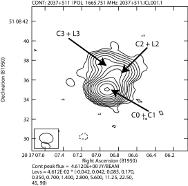
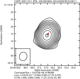
Figure 1: The components in Table 1 are identified in this 1.66 GHz VLA A-array image (top panel). The 330 MHz A-array image (bottom panel) is very slightly resolved in the North-South direction. The red line indicates the jet from C0 to C2.

3 Low Frequency Radio Observations

In this section, we discuss about the archival 151 MHz Giant Metrewave Radio Telescope (GMRT) data and the newly reduced 330 MHz VLA data, in combination with previously published 1.66 GHz and 4.86 GHz VLA data, in order to segregate the lobe emission from the total flux at low frequency. The 151 MHz data is from the TGSS Alternate Data Release 1 (Intema et al., 2016). The beam width is $>20\arcsec$, much larger than the size of the source at higher frequency. The data are consistent with a point source and we choose the peak flux density of $16.50\pm 0.17$ Jy as the best estimate of the total flux of the compact radio source.

We use the 1.66 GHz VLA A-array radio image from Kharb et al. (2010) in Figure 1 in order to assess the contribution of the various components. We have made annotations based on the high resolution images at 4.86 GHz and 14.94 GHz from O’Dea et al. (1988). The beam in the top panel of Figure 1 is $1.40\arcsec\times 1.05\arcsec$ at a PA = $83.85\degr$. The core and the strong inner knot in the jet are partially resolved and are designated as C0+C1. We denote the other two components as C2+L2 and C3+L3, where C2 and C3 are the compact components seen at 4.86 GHz in O’Dea et al. (1988) and L2 and L3 are the the diffuse emission associated with these features. The component C2+L2 is identified with the lobe on the jet side. Due to projection effects of an almost pole-on orientation, the component C3+L3 could be the radio lobe on the counter jet side.

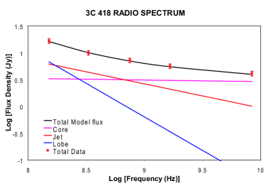
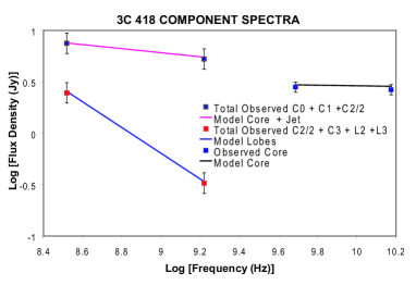
Figure 2: The Model A power law fit to the broadband radio data in Table 2 is shown in the top panel. The bottom panel shows the additional constraints of simultaneously fitting the components.

The bottom panel of Figure 1 is the 330 MHz VLA A-array image from the project AG500. These data were reduced using standard procedures in AIPS. The beam is $5.91\arcsec\times 5.27\arcsec$ at a PA = $-16.58\degr$. There is no large diffuse cloud of extended flux, but there is a slight elongation in the North-South direction in the image made with this large beam. The short red line indicates the jet path from C0 to C2 in the top panel at 1.66 GHz.

Table 1 shows the component flux densities based on model fits to the images. The 1.66 GHz image was modeled with 4 Gaussian components based on the 4 components seen at 4.86 GHz. It could be that C0 has varied significantly between the 4.86 GHz and 1.66 GHz observations, but the two epochs in O’Dea et al. (1988) showed minimal (a few per cent) variability and a very flat spectrum. We note that the separation between C0 and C1 in O’Dea et al. (1988) is much less than the beam size at 1.66 GHz. Thus, the apparent increased flux in C0 at 1.66 GHz could be just due to the blending of components. The blending of C0 and C1 at 1.66 GHz makes it hard to model the spectra of the individual components, hence they are combined in the following multi-component theoretical modeling of the source. We tried fitting the 330 MHz image with 1, 2 and 3 Gaussian components using the JMFIT task in AIPS. The best fit was with 2 components and the results are in Table 1. We list these as components A1 and A2 since it is not clear a priori which of the components in the top panel of Figure 1 are blended by these fits. Our methodology is to assume a basic blend of components, where A1 is dominated by the core and jet flux with some lobe flux and A2 is dominated by the lobe flux. The exact blend that is ultimately chosen is based on simultaneously fitting the component spectra with the 4-component theoretical power law models that we now describe.

The theoretical model fits are complicated by the fact that the observationally blended components (OBCs) and the natural theoretically blended components (TBCs), denoted below the horizontal line in Table 1, are not exactly the same. Thus, the model must simultaneously fit the decomposition of TBCs in terms of OBCs and the power laws of the individual components. We fit the TBCs separately in addition to the total flux density in Figure 2. This removes degeneracy that occurs by just fitting the total flux spectrum. We considered two classes of simple power law models in Table 2. Model A, in Figure 2, fits the core at high frequency, where it is resolved from the jet and the TBCs (in the bottom panel) as well as the total flux density (with additional data from the NASA Extragalactic Database, NED) in the top panel. Model B assumes that the core flux density is variable and is not fit separately, thus the other fits are slightly better. It is not shown because it looks similar to the model A fits.

Table 2: Model Flux Densities

Component	Flux Density	Power Law
Model A	151 MHz (Jy)	Spectral Index ($\alpha$)
Core	3.28	0.03
Jet	6.17	0.45
Lobes	6.76	1.25
Component	Flux Density	Power Law
Model B	151 MHz (Jy)	Spectral Index ($\alpha$)
Core	4.08	0.04
Jet	5.54	0.60
Lobes	6.56	1.25

The decomposition of the TBCs in terms of OBCs is simple at 330 MHz. The lobe flux density is everything except the peak flux density of A1, due to the large beam size compared to the separation ($\sim 3$ times that) between C0 and C2. The lobe flux density at 1.66 GHz is chosen to be a sum of: (1) C3+L3, (2) the integral flux density $-$ peak flux density of C2+L2 and (3) a fraction of the peak of C2+L2. Determining this fraction is the main unknown in choosing the decomposition of the TBCs in terms of OBCs, and is chosen to provide the best fit to the theoretical models. Unless the fraction is at least $\sim 0.5$ in the lobes, $\alpha$ of the lobes is unrealistically large. Conversely, full assignment to the lobes produces worse fits overall, and does not seem consistent with the jet morphology. However, it does reduce $\alpha$ to 1.05. The two conclusions of relevance are that there is clearly an excess of flux density at 151 MHz over that expected from a core-jet system, and the spectral index of the total flux is 0.77 from 151 MHz to 330 MHz. Secondly, the estimated lobe flux density and $\alpha$ are virtually identical in our two best model fits in Table 1. Thusly motivated, using Equations (1)$-$(3), we estimate that $\overline{Q}=5.5\pm 1.3\times 10^{46}\rm{ergs~{}s^{-1}}$.

4 Accretion Flow Luminosity and Black Hole Mass

Because of the bright radio core, the optical/UV spectrum might be contaminated by the tail of the synchrotron spectrum. In fact, the continuum of the optical spectrum from Smith and Spinrad (1980) corrected for Galactic extinction in NED (and the factor of 10 typographical error on the vertical axis of their spectrum) is consistent with an extrapolation of the mid-IR power law from Podigachoski et al. (2015), as indicated in Figure 3. Thus, the emission lines are a preferred method, compared to the continuum, for estimating blazar $L_{\rm{bol}}$ (Celotti et al, 1997). Using the de-reddened MgII line strength from Smith and Spinrad (1980) and the formula from Punsly et al. (2016b), $L_{\mathrm{bol}}\approx 151L(\mathrm{MgII})\approx 1.71\pm 0.85\times 10^{46}\rm{ergs~{}s^{-1}}$, where the line strength is $L(\mathrm{MgII})=1.14\pm 0.57\times 10^{44}\rm{ergs~{}s^{-1}}$. Note that the estimate does not include reprocessed radiation in the infrared from distant molecular clouds. This would be double counting the thermal accretion emission that is reprocessed at mid-latitudes (Davis and Laor, 2011).

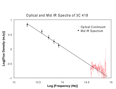
Figure 3: The continuum of the optical spectrum is consistent with a continuation of the mid-IR power law. The data has been corrected for Galactic extinction.

We independently verified the fit to the MgII line in Smith and Spinrad (1980), obtaining similar results including a full width half maximum (FWHM) of $\approx 4400$ km s^-1. We insert this value into the virial black hole mass estimates of Shen and Liu (2012) to find

$$\log\left(\frac{M_{bh}}{M_{\odot}}\right)=$$

$$3.979+0.698\log\left(\frac{L(\mathrm{MgII})}{10^{44}\,\rm{erg/s}}\right)+1.382\log\left(\frac{\rm{FWHM}}{\rm{km/s}}\right)\;,$$

$$\frac{M_{bh}}{M_{\odot}}=1.13\times 10^{9}\;.$$ (4)

Alternatively, the formula of Trakhtenbrot & Netzer (2012) yields a different estimate

$$\frac{M_{bh}}{M_{\odot}}=$$

$$6.79\times 10^{6}\left(\frac{L(\mathrm{MgII})}{10^{42}\,\rm{erg/s}}\right)^{0.5}\left(\frac{\rm{FWHM}}{1000\,\rm{km/s}}\right)^{2},$$

$$\frac{M_{bh}}{M_{\odot}}=6.37\times 10^{8}\;.$$ (5)

5 Discussion

In this paper, we analyze images at 151 MHz, 330 MHz, 1.66 GHz and 4.86 GHz in order to estimate the diffuse radio lobe flux of the core-dominated quasar 3C 418. We estimate a long term time averaged jet power of $\overline{Q}=5.5\pm 1.3\times 10^{46}\rm{ergs~{}s^{-1}}$. Using the MgII broad emission line, we estimated $L_{\mathrm{bol}}\approx 1.71\pm 0.85\times 10^{46}\rm{ergs~{}s^{-1}}$ and a central super-massive black hole mass of $M_{bh}/M_{\odot}=8.9\pm 2.4\times 10^{8}$. These results indicate a very rare state of kinetic dominance for a quasar, $1.6<\overline{Q}/L_{\rm{bol}}<7.9$ and $0.29<\overline{Q}/L_{\rm{Edd}}<0.85$. There are only $\sim 1-10$ quasars known to have $\overline{Q}/L_{\rm{bol}}$ this large (Punsly, 2007).

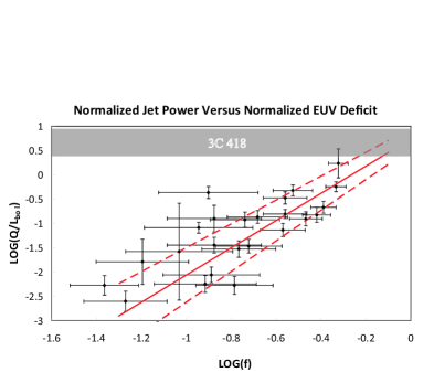
Figure 4: A log-log scatter plot of the fraction of displaced gas, $f$, versus $\overline{Q}/L_{\rm{bol}}$ (Punsly 2015). The weighted least squares fit and the standard error are the solid and dashed lines, respectively. The range of allowed values of $\overline{Q}/L_{\rm{bol}}$ for 3C 418 is indicated by the grey band.

The large value of $\overline{Q}/L_{\rm{bol}}$ is a most extreme case in the context of the extreme ultraviolet (EUV) deficit of RLQs relative to RQQs at matched far and near UV luminosity (Zheng et al., 1997; Telfer et al., 2002; Punsly, 2015). The stronger the radio jet, the steeper the spectrum of the EUV continuum, hence the deficit in the EUV for RLQs. The EUV emission originates from the innermost optically thick regions of the accretion disk, $<5M_{bh}$ (in geometrized units) from the inner edge (Punsly et al., 2016b). The steep EUV spectrum in consort with the increased jet power is explained naturally by magnetically arrested accretion (MAA) in which islands of large scale vertical magnetic flux create a Poynting flux dominated wind that removes angular momentum and energy from the innermost portions of accretion flow (Punsly, 2015). These islands are regions of suppressed turbulence that simultaneously displace the EUV emitting gas, thereby reducing the EUV emissivity which is created by turbulent dissipation in the innermost regions of the accretion disk. We denote the fraction of displaced EUV emitting gas in the innermost accretion flow by $f$. By comparing to the EUV spectra of RQQs, the fraction of displaced gas in each RLQ can be estimated. Figure 4 is a log-log scatter plot from Punsly (2015) of $f$ versus $\overline{Q}/L_{\rm{bol}}$. The plot was updated with the additional quasars added in Punsly et al. (2016a), Figure 4. The solid red line is the weighted least squares fit with uncertainty in both variables and the dashed lines are the standard error to the fit (Reed, 1989). Note that 3C 418 lies in a region that would indicate $f\mbox{\raisebox{-2.58334pt}{$\stackrel{{\scriptstyle\textstyle<}}{{\sim}}$}}1$, an almost complete saturation of the inner accretion disk by magnetic flux in the MAA model. The fact that the largest $\overline{Q}/L_{\rm{bol}}$ values implied by observations are consistent with the physically allowed maximum flux saturation is strong support for the MAA model of the EUV deficit observed empirically in RLQs.

In Punsly (2015), we discussed the different types of magnetic flux evolution that occur in various magnetically arrested simulations. The MAA dynamics posited in Punsly (2015) are based on the simulations in Igumenshchev (2008); Punsly et al. (2009) in which magnetic islands are not extremely short-lived transient features in the innermost accretion flow. The MAA scenario was shown to explain the EUV deficit of RLQs, the range of $f$ and the scaling law in Figure 4. By contrast, other simulations that are described as “magnetically arrested” in Avara et al (2016) and references therein, support magnetic islands in the innermost accretion flow, but only as rare, brief transients and therefore do not explain the EUV deficit of RLQs. The transient “prominence” states (a true magnetic island near the black hole) they describe, would need to be very common and of longer duration in order to be consistent with observation. The different simulated behaviors depend on the physical elements that determine the formation of the magnetic islands and the time evolution of the magnetic islands in the disk, reconnection and the diffusion of mass onto and off of the field lines (Igumenshchev, 2008; Punsly, 2015). The diffusion rate of plasma onto and off of magnetic field lines and magnetic reconnection rates are not well known nor well modeled near black holes. These occur in the simulations as a consequence of numerical diffusion (not a result of a realistic physical plasma model) in the over-simplified, ideal magnetohydrodynamic, single fluid models of the physics (Punsly, 2015). The observations of the EUV deficit can be a valuable guide for future physical models.

References

- Avara et al (2016) Avara, M., McKinney, J., Reynolds, C.. 2016, MNRAS, 462, 636
- Blundell and Rawlings (2000) Blundell, K., Rawlings, S. 2000, AJ 119, 1111
- Celotti et al (1997) Celotti, A., Padovani and Ghisellini, G. 1997, MNRAS, 286, 415
- Davis and Laor (2011) Davis, S., Laor, A. 2011, ApJ 728, 98
- deVries et al. (2006) deVries, W., Becker, R., White, R. 2006, AJ 131. 666
- Ganguly et al. (2007) Ganguly,, R. et al. 2007, ApJ 665, 990
- Ghisellini and Tavecchio (2015) Ghisellini, G and Tavecchio, F. 2015 MNRAS 448, 1060
- Igumenshchev (2008) Igumenshchev, I. V. 2008 ApJ 677, 317
- Intema et al. (2016) Intema, H., Jagannathan, P., Mooley, K., Frail, D. 2016 A & A http://adsabs.harvard.edu/abs/2016arXiv160304368I
- Kharb et al. (2010) Kharb, P., Lister, M., Cooper, N. 2010, ApJ 710, 764
- McNamara et al. (2011) McNamara, B., Rohanizadegan, M, and Nulsen, P. 2011, ApJ, 727, 39
- O’Dea et al. (1988) O’Dea, C., Barvainis, R. and Challis, P. 1988, AJ 96 4350
- Podigachoski et al. (2015) Podigachoski, P., Barthel, P. D., Haas, M., et al 2015, A & A 575 80
- Punsly (2005) Punsly, B. 2005, ApJL 623 L9
- Punsly (2007) Punsly, B. 2007, MNRAS Lett. 374 10
- Punsly and Tingay (2006) Punsly, B., Tingay, S. 2006, ApJL 640, 21
- Punsly et al. (2009) Punsly, B., Igumenshchev, I. V., Hirose, S. 2009 ApJ 704, 1065
- Punsly (2015) Punsly, B. 2015 ApJ 806, 47
- Punsly et al. (2016a) Punsly, B., Reynolds, C., Marziani, P., O’Dea, C. 2016a, MNRAS 459, 4233
- Punsly et al. (2016b) Punsly, B., Marziani, P., Zhang, S., Muzahid, S., O’Dea, C. 2016b, ApJ 830, 104
- Reed (1989) Reed, B. 1989, Am. J. Phys. 57, 642
- Shen and Liu (2012) Shen, Y., & Liu, X. 2012, ApJ 753, 125
- Smith and Spinrad (1980) Smith, H., Spinrad, H. 1980, ApJ 236, 419
- Telfer et al. (2002) Telfer, R., Zheng, W., Kriss, G., Davidsen, A. 2002 ApJ 565, 773
- Trakhtenbrot & Netzer (2012) Trakhtenbrot, B. and Netzer, H. 2012, MNRAS 427, 3081
- Zheng et al. (1997) Zheng, W. et al. 1997 ApJ 475, 469
- Willott et al. (1999) Willott, C., Rawlings, S., Blundell, K., Lacy, M. 1999, MNRAS 309, 1017