Transient hydrodynamic finite size effects
in simulations under periodic boundary conditions

Abstract

We use Lattice-Boltzmann and analytical calculations to investigate transient hydrodynamic finite size effects induced by the use of periodic boundary conditions in simulations at the molecular, mesoscopic or continuum levels of description. We analyze the transient response to a local perturbation in the fluid and obtain via linear response theory the local velocity correlation function. This new approach is validated by comparing the finite size effects on the steady-state velocity with the known results for the diffusion coefficient. We next investigate the full time-dependence of the local velocity auto-correlation function. We find at long times a cross-over between the expected $t^{-3/2}$ hydrodynamic tail and an oscillatory exponential decay, and study the scaling with the system size of the cross-over time, exponential rate and amplitude, and oscillation frequency. We interpret these results from the analytic solution of the compressible Navier-Stokes equation for the slowest modes, which are set by the system size. The present work not only provides a comprehensive analysis of hydrodynamic finite size effects in bulk fluids, but also establishes the Lattice-Boltzmann method as a suitable tool to investigate such effects in general.

It is by now well established that hydrodynamic finite size effects arise in simulations due to the use of periodic boundary conditions (PBC). These effects can be understood as the result of spurious hydrodynamic interactions between particles and their periodic images. Following Dünweg and Kremer Dünweg and Kremer (1993), Yeh and Hummer Yeh and Hummer (2004) proposed a complete analysis of the finite size effect on the diffusion coefficient of fluid particles in a cubic box based on the mobility tensor $\mathbb{T}$:

$$\mathbb{D}_{\rm PBC} =D_{\infty}\mathbbm{1}+k_{B}T\lim_{r\to 0}\left[\mathbb{T}_{\rm PBC}({\bf r})-\mathbb{T}_{\infty}({\bf r})\right]\,,$$ (1)

with $k_{B}$ Boltzmann’s constant and $T$ the temperature and where PBC and $\infty$ subscript denote properties under periodic and unbounded conditions, respectively, while $\mathbbm{1}$ is the identity matrix. This results in a finite size scaling of the diffusion constant $D(L)=D_{\infty}-\xi k_{B}T/6\pi\eta L$ for a cubic box of size $L$, with $\xi\approx 2.837$ a constant and $\eta$ the fluid viscosity. The same scaling was found independently Fushiki (2003) and has been confirmed in molecular dynamics simulations of a number of simple fluids Yeh and Hummer (2004), including several water models Tazi et al. (2012); Rozmanov and Kusalik (2012), ionic liquids Gabl et al. (2012) or more complex fluids such as solutions of star polymers Singh et al. (2014). More recently, the extension to anisotropic boxes was also investigated Kikugawa et al. (2015a, b) and interpreted in terms of the same hydrodynamic arguments Botan et al. (2015); Vögele and Hummer (2016).

The distortion of the flow field due to the finite size of the system (and the associated use of PBC) does not only affect the diffusion coefficient $D$ of particles, but in principle all dynamical properties. In particular, hydrodynamic flows in an unbounded fluid result in long-time tails of correlations functions, e.g. as $t^{-3/2}$ for the velocity autocorrelation function (VACF) in three dimensions Ernst et al. (1971); Hansen and McDonald (2013). Such long time tails have been reported in molecular simulations for the VACF since the pioneering work of Ref. 14 (see e.g. Levesque and Ashurst (1974)) as well as in purely hydrodynamic lattice simulations for the VACF or other correlation functions van der Hoef and Frenkel (1990); Lowe et al. (1995); van der Hoef and Frenkel (1995); Lowe and Frenkel (1995). Such slow hydrodynamic modes also manifest themselves in the non-Markovian dynamics of solutes, which includes a deterministic component of the force exerted by the suspending fluid, well described for colloidal spheres by the Basset-Boussinesq force Boussinesq (1901); Chow and Hermans (1972). Simulations displaying such a hydrodynamic memory, either on a coarse-grained Franosch et al. (2011) or molecular Lesnicki et al. (2016) scale, may therefore suffer from artefacts associated with the use of PBC, at least on long time scales. This was already recognized by Alder and Wainwright in their seminal paper where they reported their results “up to the time where serious interference between neighbouring periodically repeated systems is indicated” Alder and Wainwright (1970).

Here we address this issue of finite size effects on the transient regime by revisiting the above hydrodynamic approach. We investigate the transient response to a singular perturbation of the fluid, previously considered to predict the steady-state mobility Hasimoto (1959); Yeh and Hummer (2004). More precisely, we determine numerically the time-dependent Green’s function for the Navier-Stokes equation using Lattice Boltzmann simulations Succi (2001). We validate this new approach in the steady-state by comparison with known results, before turning to finite size effects on the transient hydrodynamic response. We show that the multiple features of these finite size effects can be rationalized analytically by considering the decay of the relevant hydrodynamic modes.

The dynamics of an incompressible fluid of mass density $\rho_{m}$ and shear viscosity $\eta$ can be described by the mass conservation $\partial_{t}\rho_{m}+\rho_{m}\nabla\cdot{\bf v}=0$ and Navier-Stokes (NS) equation:

$$\rho_{m}\frac{\partial{\bf v}}{\partial t}+\rho_{m}({\bf v}\cdot\nabla){\bf v} =\eta\nabla^{2}{\bf v}-\nabla p+\mathbf{f}$$ (2)

where ${\bf v}$ is the velocity field, $p$ is the pressure and $\mathbf{f}$ is a force density. In the limit of small Reynolds number, defined as $Re=\frac{||\rho_{m}({\bf v}\cdot\nabla){\bf v}||}{||\eta\nabla^{2}{\bf v}||}\sim\frac{uL}{\nu}$ with $u$ and $L$ the typical velocity and length, and $\nu=\eta/\rho_{m}$ the kinematic visscosity, the expression of both tensors in Eq. (1) can be obtained by determining the Green’s function for the Stokes equation. This corresponds to a vanishing left hand side in Eq. (2) and a perturbation:

$$\mathbf{f}({\bf r}^{\prime}) =\left[\delta({\bf r}^{\prime}-{\bf r})-\frac{1}{V}\right]\,\mathbf{F}\;,$$ (3)

with $\delta$ the Dirac distribution, $\mathbf{F}$ a force and $V$ the volume of the system, i.e. a singular point force at ${\bf r}$ and a uniform compensating background, applied on a fluid initially at rest. The mobility tensor then follows from the steady state velocity as ${\bf v}({\bf r}^{\prime})=\mathbb{T}({\bf r}^{\prime},{\bf r})\cdot{\bf F}$. Note that the limit in Eq. (1) corresponds to ${\bf r}^{\prime}\to{\bf r}$. The result for the unbounded case is the well-known Oseen tensor $\mathbb{T}_{\infty}({\bf r})=\frac{1}{8\pi\eta r}\left(\mathbbm{1}+\frac{{\bf r}{\bf r}}{r^{2}}\right)$, while under PBC it is more conveniently expressed in Fourier space Yeh and Hummer (2004).

Similarly, the full dynamical response can be obtained by considering a perturbation of the form $\mathbf{f}({\bf r}^{\prime})\Theta(t)$, where $\Theta(t)$ is the Heaviside function and the spatial dependence is given by Eq. (3), applied on a fluid initially at rest. The Green’s function for the time-dependent NS equation, which corresponds to a perturbation $\mathbf{f}({\bf r}^{\prime})\delta(t)$ is obtained as the time-derivative of the solution ${\bf v}(r^{\prime},t)$. In the limit $Re\ll 1$, the response to $\mathbf{f}({\bf r}^{\prime})\Theta(t)$ converges at long times toward the stationary field corresponding to the mobility tensor.

The transient hydrodynamic regime, as quantified by the Green’s function, is also related to the equilibrium fluctations of the velocity field. Using linear response theory Hansen and McDonald (2013), it is easy to show that the average velocity $v$ (in the sense of a canonical average over initial configurations) in the direction of the force at the position where it is applied, evolves as: $\frac{d}{dt}\left\langle\displaystyle v({\bf r},t)\right\rangle=\frac{1}{k_{B}T}\int d{\bf r}^{\prime}\left\langle\displaystyle v({\bf r},t)v({\bf r}^{\prime},0)\right\rangle f({\bf r}^{\prime},t)$. This simplifies for the perturbation considered in Eq. (3), since the total applied force vanishes and so does the total flux $\int d{\bf r}^{\prime}v({\bf r}^{\prime},0)$. One can finally express the velocity auto-correlation of the local velocity field (LVACF) as:

$$Z(t) \equiv\left\langle\displaystyle v({\bf r},t)v({\bf r},0)\right\rangle=\frac{k_{B}T}{F}\frac{d\left\langle\displaystyle v({\bf r},t)\right\rangle}{dt}\;,$$ (4)

where $\left\langle\displaystyle v({\bf r},t)\right\rangle$ is the response to the perturbation Eq. (3). Note that this expression, although similar to the one for the velocity of a particle under a constant force $F$, has in fact a very different meaning: Here a perturbation is applied at a fixed position ${\bf r}$ (together with the compensating background) and the fluid velocity is followed at that position. Integrating between 0 and infinity, one obtains the steady state velocity $v_{\infty}({\bf r})=\lim_{t\to\infty}\left\langle\displaystyle v({\bf r},t)\right\rangle=\frac{F}{k_{B}T}\int_{0}^{\infty}\left\langle\displaystyle v({\bf r},t)v({\bf r},0)\right\rangle{\rm d}t$. This relation is analoguous to Einstein’s relation for the mobility of a particle, $\mu=v/F=D/k_{B}T$, with the diffusion coefficient $D=\int_{0}^{\infty}Z(t){\rm d}t$. In the following we will therefore refer to the integral of the LVACF as the diffusion coefficient.

Here we use Lattice Boltzmann (LB) simulations Succi (2001) to solve the above hydrodynamic problem, i.e. the Navier-Stokes equation for a fluid initially at rest on which the perturbation Eq. (3) is applied. In a nutshell, the LB method evolves the one-particle velocity distribution $f({\bf r},{\bf c},t)$ from which the hydrodynamic moments (density, flux, stress tensor) can be computed. In practice, a kinetic equation is discretized in space (lattice spacing $\Delta x$) and time (time step $\Delta t$) and so are the velocities, which belong to a finite set $\{{\bf c}_{i}\}$ (here we use the D3Q19 lattice). The populations $f_{i}({\bf r},t)\equiv f({\bf r},{\bf c}_{i},t)$ are updated following:

$$f_{i}({\bf r}+{\bf c}_{i}\Delta t,t+\Delta t) =f_{i}({\bf r},t)$$

$$\hskip-56.9055pt-\frac{\Delta t}{\tau}\left[f_{i}({\bf r},t)-f_{i}^{eq}({\bf r},t)\right]+F_{i}^{ext}({\bf r},t)\;,$$ (5)

where $f_{i}^{eq}({\bf r},t)$ corresponds to the local Maxwell-Boltzmann equilibrium with density $\rho({\bf r},t)=\sum_{i}w_{i}f_{i}({\bf r},t)$ and flux $\rho{\bf v}({\bf r},t)=\sum_{i}w_{i}f_{i}({\bf r},t){\bf c}_{i}$, where $w_{i}$ are the weights associated with each velocity. The relaxation time $\tau$ controls the fluid viscosity. Here we use $\tau=\Delta t$, which results in a kinematic viscosity $\nu=\frac{c_{s}^{2}\Delta t}{2}=\frac{1}{6}\frac{\Delta x^{2}}{\Delta t}$ since for the D3Q19 lattice the speed of sound is $c_{s}=\frac{1}{\sqrt{3}}\frac{\Delta x}{\Delta t}$ and $F_{i}^{ext}$ accounts for the external force acting on the fluid Succi (2001). We perform simulations for orthorhombic cells with one length ($L_{\perp}$) different from the other two ($L_{\parallel}$), as illustrated in Figure 1a, in order to analyze the effect of both the system size and shape. In practice, we apply the singular perturbation to a single node of the lattice (and the compensating background everywhere) and monitor the fluid velocity on that node, as shown in Figure 1b.

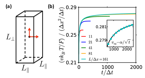
Figure 1: a. A bulk fluid in an orthorhombic cell with one length different from the other two is submitted to a perturbation Eq. (3) which corresponds to a singular point force (in one of the two relevant directions indicated by red arrows) and a uniform compensating background. Both elongated ($L_{\perp}>L_{\parallel}$, as shown) and flat ($L_{\perp}<L_{\parallel}$) boxes are considered. b. Velocity at point ${\bf r}$ where the perturbation is applied, as a function of time, from Lattice Boltzmann simulations with various cubic boxes of size $L=L_{\perp,\parallel}$. The inset shows the scaling at long times used to extrapolate the steady-state velocity, for the largest system.

As a validation of this new approach for the computation of hydrodynamic Green’s function with LB simulations and linear response, we first describe the results for the diffusion coefficient, obtained from the steady-state velocity as $D=k_{B}Tv_{\infty}({\bf r})/F$. In the considered geometry, the diffusion tensor is anisotropic and the two independent components $D_{\parallel,\perp}$ can be determined by applying the perturbation Eq. (3) in the corresponding directions. Continuum hydrodynamics predicts a scaling with system size Botan et al. (2015):

$$D_{\parallel,\perp} =D_{\infty}+\frac{k_{B}T}{6\pi\eta L_{\parallel}}h_{\parallel,\perp}\!\left(\frac{L_{\perp}}{L_{\parallel}}\right)\,,$$ (6)

where the two functions $h_{\parallel,\perp}$ depend only on the aspect ratio $L_{\perp}/L_{\parallel}$. Both functions have been determined in Ref. Botan et al. (2015). For the isotropic case $h_{\parallel,\perp}(1)=-\xi\approx-2.837$. The inset of Figure 2 shows the diffusion coefficient for a cubic box as a function of the size $L_{\perp}=L_{\parallel}$. For reasons that will be discussed below, the velocity $\left\langle\displaystyle v({\bf r},t)\right\rangle$ converges slowly to its steady-state value, as $v_{\infty}-\alpha/\sqrt{t}$ (see the inset of Figure 1b). Therefore we used a fit to this expression at long times in order to determine $v_{\infty}$ for the larger systems. For small systems the convergence is faster so that such an extrapolation is not necessary.

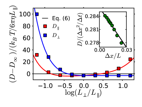
Figure 2: Scaling functions $h_{\parallel,\perp}=(D_{\parallel,\perp}-D_{\infty})/(k_{B}T/6\pi\eta L_{\parallel})$ defined in Eq. (6) as a function of the aspect ratio $\alpha=L_{\perp}/L_{\parallel}$. Lattice Bolzmann results (symbols) are compared to analytical results (lines) from Ref. 10. Note the logarithmic scale on the $x$-axis. Each point corresponds to the slope of a scaling with system size at fixed aspect ratio, as illustrated in the inset for a cubic box ($L=L_{\perp,\parallel}$), where the line again corresponds to Eq. (6).

The LB results are in excellent agreement with the slope expected from Eq. (6), even though some deviations are observed for the smaller box sizes ($\sim 10\Delta x$) as expected. The extrapolated value for an infinite system is $D_{\infty}\approx 0.286\Delta x^{2}/\Delta t$. By performing similar size scalings for various aspect ratios Sup , we can compute the scaling functions $h_{\parallel,\perp}$ for both components of the diffusion tensor. The results, shown in the main part of Figure 2, are also in excellent agreement with Eq. (6). This validates the present approach combining linear response and LB simulations for the determination of hydrodynamic finite size effects on the steady-state dynamics.

We now turn to the finite size effects in the transient regime. As explained above, the Green’s function for the time-dependent NS equation is obtained from the derivative of the response $v({\bf r},t)$ to the perturbation ${\bf f}({\bf r}^{\prime})\Theta(t)$. More precisely, we discuss here the LVACF defined by Eq. (4) which is proportional to this Green’s function and quantifies the equilibrium hydrodynamic fluctuations. In an unbounded medium, such fluctuations are known to result in the long-time tail of the VACF of particles in a simple fluid according to Hansen and McDonald (2013):

$$Z_{\infty}(t) =\frac{2}{3}\frac{k_{B}T}{\rho_{m}}\left[4\pi\nu t\right]^{-3/2}\;.$$ (7)

Mode-coupling theory predicts in fact a scaling with $D+\nu$ instead of $\nu$, but here the Green’s function is not associated with the diffusion of a tagged particle, so that the corresponding diffusion coefficient is not involved.

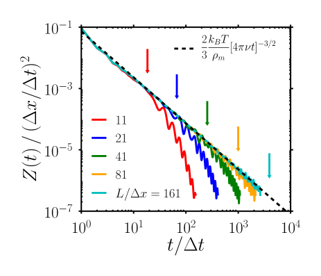
Figure 3: Local velocity auto-correlation function (LVACF) computed from Lattice Boltzmann simulations in a cubic cell, for various cell sizes $L/\Delta x$. The double logarithmic scale underlines the algebraic decay expected from hydrodynamics in an unbounded fluid, Eq. (7). The finite size results in a cross-over to an exponential decay, analyzed in further detail in Figure 4. The arrows indicate the diffusion time for the slowest mode, $\tau_{L}=1/\nu k_{L}^{2}$, with $k_{L}=2\pi/L$, which corresponds to the exponential decay rate and is also typical of the cross-over between the algebraic and exponential regimes.

Figure 3 reports the LVACF computed from Eq. (4) using the present LB approach, for various cubic boxes of size $L$. For the larger systems, the simulation results coincide exactly with the hydrodynamic scaling Eq. (7) over several orders of magnitude, without any ajustable parameter. This scaling, together with Eq. (4), justifies a posteriori the fit of the velocity as $v_{\infty}-\alpha/\sqrt{t}$ to extrapolate the steady-state value. However, we observe a cross-over from the algebraic decay to an exponential regime (and oscillations discussed in more detail below), with a cross-over time that decreases with decreasing $L$.

It is useful to recall that the algebraic decay Eq. (7) results from the superposition of an infinite number of modes (corresponding to the hydrodynamic limit of vanishing wave numbers $k\to 0$) for momentum diffusion, which in Fourier space decay as $\sim e^{-\nu k^{2}t}$. The exponential decay therefore results from the cut-off at low wave numbers introduced by the PBC, with the slowest mode corresponding to $k_{L}=2\pi/L$ and a characteristic time $\tau_{L}=1/\nu k_{L}^{2}$. The vertical arrows in Figure 3, which indicate this time, show that it is also typical of the cross-over from algebraic to exponential decay $A_{L}e^{-\nu k_{L}^{2}t}$ of the LVACF. The prefactor $A_{L}$ can be roughly estimated by assuming the continuity between the two regimes at $t=\tau_{L}$. Using Eq. (7), this results in:

$$A_{L} =\frac{2e}{3\left[4\pi\right]^{3/2}}\frac{k_{B}T}{\rho_{m}}k_{L}^{3}\;.$$ (8)

Another striking feature of the results in Figure 3 is the presence of oscillations, with a frequency which depends on the size of the simulation box. This is clearly another finite size effect, which can be understood in terms of the slight compressibility of the fluid. Indeed, in the LB method the fluid is only quasi-incompressible. In such a case, while the transverse mode decays as $\sim e^{-\nu k^{2}t}$ (as for an incompressible fluid), the longitudinal modes follow a dispersion relation which can be obtained by linearizing the mass conservation and compressible NS equation, for an isothermal perturbation of the form $e^{i(\omega t-{\bf k}\cdot{\bf r})}$. Using the fact that the equation of state of the LB fluid is that of an ideal gas ($p=\rho k_{B}T=\rho_{m}c_{s}^{2}$), one obtains the following dispersion relation: $(i\omega)^{2}+i\omega k^{2}\left(\frac{4}{3}\nu+\nu^{\prime}\right)+c_{s}^{2}k^{2}=0$, with $\nu^{\prime}=\zeta/\rho_{m}$ the kinematic bulk viscosity. In the case of the D3Q19 lattice, for which $\nu^{\prime}=\frac{2}{3}\nu$, the solutions are of the form $i\omega=-\nu k^{2}\pm ikc_{s}\sqrt{1-\nu^{2}k^{2}/c_{s}^{2}}\sim-\nu k^{2}\pm ikc_{s}$ (for $k\ll c_{s}/\nu$), i.e. attenuated sound waves. Such a dispersion relation had already been considered for the LB simulation of acoustic waves, see e.g. Dellar (2001); Li and Shan (2011); Viggen (2011).

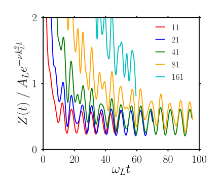
Figure 4: Local velocity autocorrelation function computed from Lattice Boltzmann simulations in a cubic cell, for various cell sizes $L/\Delta x$, normalized by the expected exponential scaling at long times $A_{L}e^{-\nu k_{L}^{2}t}$ with $k_{L}=2\pi/L$ and $A_{L}$ given by Eq. (8), as a function of time rescaled by the frequency $\omega_{L}=kc_{s}\sqrt{1-\nu^{2}k^{2}/c_{s}^{2}}$. The oscillations are due to the small compressibility of the Lattice-Boltzmann fluid, which results in damped acoustic waves. For the larger systems the contribution of slower modes $nk_{L}$ is still visible on the time scale of the simulations.

For periodic systems, the slowest modes correspond to $k_{L}=2\pi/L$ and longitudinal modes decay as $\sim e^{-\nu k_{L}^{2}t}\cos{\omega_{L}t}$, with a frequency $\omega_{L}=k_{L}c_{s}\sqrt{1-\nu^{2}k_{L}^{2}/c_{s}^{2}}\sim k_{L}c_{s}$. Figure 4 reports the LVACF normalized by the exponential decay $A_{L}e^{-\nu k_{L}^{2}t}$, as a function of the rescaled time $\omega_{L}t$, for various system sizes spanning more than one order of magnitude. The numerical results clearly show that the above analysis captures all the main features of the finite size effects on the transient hydrodynamic response: 1) the rate of the exponential decay, since at long times the curves oscillate around a plateau; 2) the order of magnitude $A_{L}$ of the exponential regime, since the value of the plateau is the same for all system sizes; 3) the frequency of the oscillations, which are in phase after rescaling by $\omega_{L}$. While only the slowest mode contributes to the oscillations for the smallest system ($L=11\Delta x$), others are increasingly visible in this time range as the system size increases. Indeed, the other modes $nk_{L}$ decay as $\sim e^{-\nu n^{2}k_{L}^{2}t}=e^{-\frac{\nu n^{2}k_{L}^{2}}{\omega_{L}}\omega_{L}t}$, i.e. $\frac{\nu n^{2}k_{L}^{2}}{\omega_{L}}=n^{2}\frac{\nu k_{L}}{c_{s}}$ times faster – a difference which decreases with increasing $L$.

Overall, the present work shows that it is possible to rationalize all finite size effects in terms of the cut-off of hydrodynamic modes at small wave numbers introduced by the use of PBC. Coming back to Alder and Wainwright’s quote Alder and Wainwright (1970), the time where neighbouring periodically repeated systems seriously interfere corresponds to momentum diffusion time for the slowest mode, $\tau_{L}=1/\nu k_{L}^{2}$. It is crucial for the setup and analysis of molecular simulations to have a good control of these finite size effects, which can be efficiently computed from the present approach combining linear response and Lattice-Boltzmann simulations. In turn, such an analysis is useful to extrapolate the macroscopic limit without actually performing the simulations for too large systems. One could exploit these effects further to determine material properties, not only the viscosity from the slope of the diffusion coefficient vs inverse box size (as for water in first principles molecular dynamics simulations Kühne et al. (2009)), but also e.g. the speed of sound from the oscillation frequency of the LVACF, as shown here.

The systematic finite size analysis of the transient response of bulk fluids could also be extended to other situations, such as fluids under confinement or near interfaces. For example, the long-time decay of the VACF under confinement or near a boundary, in an otherwise unbounded fluid, scales as $t^{-5/2}$ instead of $t^{-3/2}$ in the bulk Hagen et al. (1997); Huang and Szlufarska (2015), but PBC in the directions parallel to the interface will also result in deviations from the algebraic decay, as demonstrated here. Similarly, it has been recently shown that the diffusion coefficient of lipids and carbon nanotubes embedded in a membrane diverges logarithmically with system size Vögele and Hummer (2016) and one should also observe the impact of PBC on the transient dynamics. This may also prove important for extracting from finite size simulations other dynamical properties for which hydrodynamics play an important role, such as memory kernels Lesnicki et al. (2016).

References

- Dünweg and Kremer (1993) Burkhard Dünweg and Kurt Kremer, “Molecular dynamics simulation of a polymer chain in solution,” The Journal of chemical physics 99, 6983–6997 (1993).
- Yeh and Hummer (2004) In-Chul Yeh and Gerhard Hummer, “System-Size Dependence of Diffusion Coefficients and Viscosities from Molecular Dynamics Simulations with Periodic Boundary Conditions,” The Journal of Physical Chemistry B 108, 15873–15879 (2004).
- Fushiki (2003) M. Fushiki, “System size dependence of the diffusion coefficient in a simple liquid,” Physical Review E 68 (2003).
- Tazi et al. (2012) S. Tazi, A. Boţan, M. Salanne, V. Marry, P. Turq, and B. Rotenberg, “Diffusion coefficient and shear viscosity of rigid water models,” Journal of Physics: Condensed Matter 24, 284117 (2012).
- Rozmanov and Kusalik (2012) Dmitri Rozmanov and Peter G. Kusalik, “Transport coefficients of the TIP4p-2005 water model,” The Journal of Chemical Physics 136, 044507 (2012).
- Gabl et al. (2012) Sonja Gabl, Christian Schröder, and Othmar Steinhauser, “Computational studies of ionic liquids: Size does matter and time too,” The Journal of Chemical Physics 137, 094501 (2012).
- Singh et al. (2014) Sunil P. Singh, Chien-Cheng Huang, Elmar Westphal, Gerhard Gompper, and Roland G. Winkler, “Hydrodynamic correlations and diffusion coefficient of star polymers in solution,” The Journal of Chemical Physics 141, 084901 (2014).
- Kikugawa et al. (2015a) Gota Kikugawa, Shotaro Ando, Jo Suzuki, Yoichi Naruke, Takeo Nakano, and Taku Ohara, “Effect of the computational domain size and shape on the self-diffusion coefficient in a Lennard-Jones liquid,” The Journal of chemical physics 142, 024503 (2015a).
- Kikugawa et al. (2015b) Gota Kikugawa, Takeo Nakano, and Taku Ohara, “Hydrodynamic consideration of the finite size effect on the self-diffusion coefficient in a periodic rectangular parallelepiped system,” The Journal of Chemical Physics 143, 024507 (2015b).
- Botan et al. (2015) Alexandru Botan, Virginie Marry, and Benjamin Rotenberg, “Diffusion in bulk liquids: finite-size effects in anisotropic systems,” Molecular Physics 113, 2674–2679 (2015).
- Vögele and Hummer (2016) Martin Vögele and Gerhard Hummer, “Divergent Diffusion Coefficients in Simulations of Fluids and Lipid Membranes,” The Journal of Physical Chemistry B 120, 8722 8732 (2016).
- Ernst et al. (1971) M. H. Ernst, E. H. Hauge, and J. M. J. Van Leeuwen, “Asymptotic time behavior of correlation functions. I. Kinetic terms,” Physical Review A 4, 2055 (1971).
- Hansen and McDonald (2013) J.-P. Hansen and I.R. McDonald, Theory of Simple Liquids, 4th Edition (Academic Press, 2013).
- Alder and Wainwright (1967) B. J. Alder and T. E. Wainwright, “Velocity autocorrelations for hard spheres,” Physical review letters 18, 988 (1967).
- Levesque and Ashurst (1974) D. Levesque and W.T. Ashurst, “Long-Time Behavior of the Velocity Autocorrelation Function for a Fluid of Soft Repulsive Particles,” Physical Review Letters 33, 277 (1974).
- van der Hoef and Frenkel (1990) M. A. van der Hoef and D. Frenkel, “Long-time tails of the velocity autocorrelation function in two- and three-dimensional lattice-gas cellular automata: A test of mode-coupling theory,” Physical Review A 41, 4277–4284 (1990).
- Lowe et al. (1995) C. P. Lowe, D. Frenkel, and A. J. Masters, “Long-time tails in angular momentum correlations,” The Journal of Chemical Physics 103, 1582–1587 (1995).
- van der Hoef and Frenkel (1995) Martin A. van der Hoef and Daan Frenkel, “Computer simulations of long-time tails: What’s new?” Transport Theory and Statistical Physics 24, 1227–1247 (1995).
- Lowe and Frenkel (1995) C. P. Lowe and D. Frenkel, “The super long-time decay of velocity fluctuations in a two-dimensional fluid,” Physica A: Statistical Mechanics and its Applications 220, 251–260 (1995).
- Boussinesq (1901) J Boussinesq, Théorie Analytique de la Chaleur (Vol. 2) (1901).
- Chow and Hermans (1972) T. S. Chow and J. J. Hermans, “Effect of Inertia on the Brownian Motion of Rigid Particles in a Viscous Fluid,” The Journal of Chemical Physics 56, 3150 (1972).
- Franosch et al. (2011) Thomas Franosch, Matthias Grimm, Maxim Belushkin, Flavio M. Mor, Giuseppe Foffi, László Forró, and Sylvia Jeney, “Resonances arising from hydrodynamic memory in Brownian motion,” Nature 478, 85–88 (2011).
- Lesnicki et al. (2016) Dominika Lesnicki, Rodolphe Vuilleumier, Antoine Carof, and Benjamin Rotenberg, “Molecular Hydrodynamics from Memory Kernels,” Physical Review Letters 116, 147804 (2016).
- Alder and Wainwright (1970) B. J. Alder and T. E. Wainwright, “Decay of the velocity autocorrelation function,” Physical review A 1, 18 (1970).
- Hasimoto (1959) H. Hasimoto, “On the periodic fundamental solutions of the Stokes equations and their application to viscous flow past a cubic array of spheres,” Journal of Fluid Mechanics 5, 317–328 (1959).
- Succi (2001) S. Succi, The Lattice Boltzmann Equation for Fluid Dynamics and Beyond (Oxford University Press, 2001).
- (27) “See supplemental material at [url will be inserted by publisher] for the list of simulated systems.” .
- Dellar (2001) Paul J. Dellar, “Bulk and shear viscosities in lattice Boltzmann equations,” Physical Review E 64 (2001).
- Li and Shan (2011) Y. Li and X. Shan, “Lattice Boltzmann method for adiabatic acoustics,” Philosophical Transactions of the Royal Society A: Mathematical, Physical and Engineering Sciences 369, 2371–2380 (2011).
- Viggen (2011) Erlend Magnus Viggen, “Viscously damped acoustic waves with the lattice Boltzmann method,” Philosophical Transactions of the Royal Society of London A: Mathematical, Physical and Engineering Sciences 369, 2246–2254 (2011).
- Kühne et al. (2009) Thomas D. Kühne, Matthias Krack, and Michele Parrinello, “Static and Dynamical Properties of Liquid Water from First Principles by a Novel Car-Parrinello-like Approach,” Journal of Chemical Theory and Computation 5, 235–241 (2009).
- Hagen et al. (1997) M. H. J. Hagen, I. Pagonabarraga, C. P. Lowe, and Daan Frenkel, “Algebraic decay of velocity fluctuations in a confined fluid,” Physical review letters 78, 3785 (1997).
- Huang and Szlufarska (2015) Kai Huang and Izabela Szlufarska, “Effect of interfaces on the nearby Brownian motion,” Nature Communications 6, 8558 (2015).