Theta dependence in the large N limit

Abstract:

Studies of the large $N$ behaviour of the topological properties of gauge theories typically focused on the large $N$ scaling of the topological susceptibility. A much more difficult task is the study of the behaviour of higher cumulants of the topological charge in the large $N$ limit, which up to now remained elusive. We will present first results confirming the expected large $N$ scaling of the coefficient commonly denoted by $b_{2}$, related to the kurtosis of the topological charge.

1 Introduction

In recent times there has been a renewed interest in the $\theta$ dependence of gauge theories: this topic emerges naturally in several approaches to the physics of strongly interacting matter, both theoretically oriented (like semiclassical methods, expansion in the number of colors, holographic and lattice methods) and phenomenologically relevant (like $U_{A}(1)$ problem, $\eta^{\prime}$ physics and axions). The euclidean Lagrangian of gauge theories in the presence of a non-vanishing $\theta$ parameter is

$$\mathcal{L}_{\theta}=\frac{1}{4}F_{\mu\nu}^{a}(x)F_{\mu\nu}^{a}(x)-i\theta q(x)\ ,\qquad q(x)=\frac{g^{2}}{64\pi^{2}}\epsilon_{\mu\nu\rho\sigma}F_{\mu\nu}^{a}(x)F_{\rho\sigma}^{a}(x)\ ,$$ (1)

where $q(x)$ is the topological charge density, whose four-dimensional integral is (for smooth configurations with finite action) an integer number: the topological charge $Q$.

Since $q(x)$ can be written as the four-divergence of the Chern-Simons current, the theory is in fact independent of $\theta$ both at the classical and at the perturbative quantum level; nevertheless nonperturbative quantum effects induce a dependence of observables on the $\theta$ value. Of particular interest is the dependence on $\theta$ of the ground state energy density $E$ (or at finite temperature of the free energy density $F$), which can be parametrized in the form (see e.g. [1])

$$E(\theta)-E(0)=\frac{1}{2}\chi\theta^{2}\big{(}1+b_{2}\theta^{2}+b_{4}\theta^{4}+\cdots\big{)}\ ,$$ (2)

where $\chi$ is, by definition, the topological susceptibility of the theory and the coefficients $b_{2n}$s characterize deviations from the leading quadratic behaviour.

This expansion is expected to have a finite radius of convergence, however no generic analytical method is known to compute the coefficients $\chi,b_{2n}$s from first principles with a systematically improvable precision. A systematic framework for evaluating $\chi$ and $b_{2n}$s by means of numerical simulations is instead provided by the lattice discretization of the theory, although some difficulties are encountered, as will be discussed in the next sections.

A drastic simplification of the $\theta$ dependence of the ground state energy density happens in the limit of an infinite number of colors: it is in fact quite easy to obtain, using standard large $N$ scaling arguments (see [1, 4]), the relations

$$\chi(N)=\bar{\chi}+O(N^{-2}),\quad b_{2n}(N)=\bar{b}_{2n}N^{-2n}+O(N^{-2n-2})\ ,$$ (3)

where $\bar{\chi}$ and $\bar{b}_{2n}$ are $N$-independent numbers. From these relations it follows that, in the limit of a large number of colors, $\chi\to\bar{\chi}$ and $b_{2n}\to 0$. It has however to be explicitly remarked that the relations Eq (3) are not expected to be universally valid: they are obtained by assuming that $\bar{\theta}=\theta/N$ is the correct scaling variable in the large $N$ limit, which follows from the assumption that $\lim_{N\to\infty}\chi(N)$ is not singular (i.e. not vanishing nor divergent). When numerically verifying the first and the second of Eq. (3) one is in fact checking two different aspects: by checking that the first equation is satisfied with $0<\bar{\chi}<\infty$ one confirms the basic hypothesis used to study the $\theta$ dependence in the large $N$ limit (and that is needed for the solution of the $U_{A}(1)$ problem), when checking the second relation one is verifying the internal consistency of this hypothesis.

The main aim of all the past studies concerning the large $N$ behaviour of the $\theta$ dependence was the study of $\chi(N)$; a notable exception is the study by Del Debbio et al. in [5], in which first results for $b_{2}$ in the $N=3,4,6$ cases were reported, but the precision was too poor to draw firm conclusions from data. On the other hand several studies later investigated the value of $b_{2}$ for the case of $SU(3)$, obtaining nicely compatible results and reaching a relative precision around $7\%$ (see Fig. 6 of [6]). In the following we will discuss the main ideas and results of the work [7] (to which we refer for more details), in which the scaling relation for $b_{2}$ in Eq (3) was for the first time numerically confirmed.

2 Numerical setup

The standard way of computing the coefficients $\chi$ and $b_{2n}$s appearing in Eq. (2) is to study the cumulants of the distribution of the topological charge $Q$ at $\theta=0$. It is indeed easy to show that the lowest order coefficients are given by (odd momenta vanish because of the $CP$ invariance at $\theta=0$)

$$\chi=\frac{\langle Q^{2}\rangle_{\theta=0}}{\mathcal{V}},\quad b_{2}=-\frac{\langle Q^{4}\rangle_{\theta=0}-3\langle Q^{2}\rangle^{2}_{\theta=0}}{12\langle Q^{2}\rangle_{\theta=0}},$$ (4)

$$b_{4}=\frac{\left[\langle Q^{6}\rangle-15\langle Q^{2}\rangle\langle Q^{4}\rangle+30\langle Q^{2}\rangle^{3}\right]_{\theta=0}}{360\langle Q^{2}\rangle_{\theta=0}}\ ,$$

where $\mathcal{V}$ is the four-dimensional volume. From these expressions it follows that the topological susceptibility is the variance of the $Q$ distribution, while the $b_{2n}$s coefficients parametrize the deviations from a Gaussian distribution.

The last sentence often causes some confusion due to the fact that, by the central limit theorem, the distribution of $Q$ becomes closer and closer to a Gaussian in the thermodynamic limit and one could erroneously guess the $b_{2n}$s coefficients to vanish in this limit. However the central limit theorem just states that the probability distribution of the variable $Q/\sqrt{\mathcal{V}}$ pointwise converges to a Gaussian distribution, and this does not imply that the cumulants of the non rescaled variable $Q$ (the ones appearing in the numerators of Eq. (4)) vanishes. In fact these cumulants are extensive, in such a way that the $b_{2n}$s are intensive quantities, as should be clear from Eq. (2).

The central limit theorem however has important consequences on the scaling with the volume of Monte Carlo errors: it is intuitively clear that the estimator of a quantity measuring the deviation from a Gaussian distribution will be noisier and noisier as the volume is increased. This can be easily formalized (see e.g. [6]) and the outcome is that, at fixed Monte Carlo statistics, the error of the $b_{2n}$ estimator at $\theta=0$ grows with the volume like $\mathcal{V}^{n}$. The way out of this lacking of self-averaging is well know [8]: instead of evaluating fluctuation observables at vanishing external field, one has to study the response to an external source. In the present context, an external source is a non-zero value of the $\theta$ parameter, that has to be imaginary in order not to spoil the reality of the action: $\theta=-i\theta_{I}$. It is then easy to show that [9]

$$\frac{\langle Q\rangle_{\theta_{I}}}{\mathcal{V}}=\chi\theta_{I}(1-2b_{2}\theta_{I}^{2}+3b_{4}\theta_{I}^{4}+\ldots)\ ,$$ (5)

from which it follows that $\chi$ and the $b_{2n}$s coefficients can be extracted, e.g., from the $\theta$ dependence of the average $\langle Q\rangle_{\theta_{I}}$, whose error does not grow with the volume.

3 Numerical results

The discretized action adopted in the simulations was

$$S[U]=S_{W}[U]-\theta_{L}Q_{L}[U]\,,$$ (6)

where $S_{W}$ is the Wilson action, $Q_{L}=\sum_{x}q_{L}(x)$ and $q_{L}(x)$ is the simplest discretization of the topological charge density with definite parity:

$$q_{L}(x)=-\frac{1}{2^{9}\pi^{2}}\sum_{\mu\nu\rho\sigma=\pm 1}^{\pm 4}{\tilde{\epsilon}}_{\mu\nu\rho\sigma}\hbox{Tr}\left(\Pi_{\mu\nu}(x)\Pi_{\rho\sigma}(x)\right)\ .$$ (7)

In the last expression $\Pi_{\mu\nu}$ denotes the plaquette while $\tilde{\epsilon}_{\mu\nu\rho\sigma}$ is an extension of the usual Levi-Civita tensor, defined for negative entries by ${\tilde{\epsilon}}_{\mu\nu\rho\sigma}=-{\tilde{\epsilon}}_{(-\mu)\nu\rho\sigma}$ and complete antisymmetry. This simple discretization makes the MC update easier, however it has the disadvantage of inducing a finite renormalization of the lattice operator $q_{L}$ [10], which translate in a finite renormalization of the lattice $\theta$ parameter: $\theta_{I}=Z(a)\theta_{L}$ (where $a$ is the lattice spacing).

To avoid the appearance of further renormalizations also in the observables, the topological charge $Q_{L}$ was measured after cooling [11] (see [12] for discussions about the equivalence of different smoothing algorithms, like gradient-flow), and in particular the following prescription was used to assign to a configuration a value of the topological charge:

$$Q=\mathrm{round}\left(\alpha\,Q_{L}^{\rm cool}\right)\ ,$$ (8)

where $\mathrm{round}(\cdot)$ denotes the truncation to the closest integer and the coefficient $\alpha$ is defined in such a way to make $\alpha Q_{L}^{\rm cool}$ on average as close as possible to the integer values (see [7] for more details).

Measures have been performed after several cooling steps (ranging from 5 to 25), in order to check for the stability of the results, and the values of $Z$, $\chi$, $b_{2}$ and $b_{4}$ have been extracted by fitting the first four cumulants of $Q$ according to the relations:

$$\begin{split}\frac{\langle Q\rangle_{\theta_{L}}}{\mathcal{V}}&=\chi Z\theta_{L}(1-2b_{2}Z^{2}\theta_{L}^{2}+3b_{4}Z^{4}\theta_{L}^{4}+\dots)\,,\\ \frac{\langle Q^{2}\rangle_{\theta_{L},c}}{\mathcal{V}}&=\chi(1-6b_{2}Z^{2}\theta_{L}^{2}+15b_{4}Z^{4}\theta_{L}^{4}+\dots)\,,\\ \frac{\langle Q^{3}\rangle_{\theta_{L},c}}{\mathcal{V}}&=\chi(-12b_{2}Z\theta_{L}+60b_{4}Z^{3}\theta_{L}^{3}+\dots)\,,\\ \frac{\langle Q^{4}\rangle_{\theta_{L},c}}{\mathcal{V}}&=\chi(-12b_{2}+180b_{4}Z^{2}\theta_{L}^{2}+\dots)\,.\end{split}$$ (9)

In order to check for systematics, different truncations of these equations have been tested. By keeping all the terms up to $\theta^{6}$ in the expansion of $E(\theta)$ it was possible to obtain estimates for all the coefficients up to $b_{4}$ (with the $b_{4}$ values that always turned out to be compatible with zero). Compatible results for $Z$, $\chi$ and $b_{2}$ were obtained in all the cases by using a truncation to $O(\theta^{4})$, see Fig. 1 (left) for the example of the $SU(6)$ case. The use of the imaginary $\theta$ source enabled us to reach very large physical volumes (up to $L\sqrt{\sigma}\gtrsim 4$) and to exclude the presence of any sizable finite volume effects, see Fig. 1 (right).

To continuum extrapolate the results we used a fit adopting the leading $O(a^{2})$ correction and checking for systematics by varying the fit range. This was done in all the cases but for $b_{2}$ in the $SU(6)$ case; in this case no sizable dependence on lattice spacing was observed for $a^{2}\sigma\lesssim 0.1$ (that was the continuum scaling region used for the other $N$ values) and the conservative estimate $-0.0045(15)$ was used (for more details and tables of numerical values see [7]).

In Fig. 2 (left) we report the $N$ dependence of the continuum extrapolated ratio $\chi/\sigma^{2}$, that nicely follows the theoretical expectations. By using the scaling form in Eq. (3) we obtained $(\chi/\sigma^{2})|_{\infty}=0.0209(11)$, a result compatible with the previous determinations [5] and only slightly more accurate. Indeed most of the error comes from the string tension and using a different scale setting observable would be sufficient to significantly improve the final error; since our main interest was the dimensionless quantity $b_{2}$ we did not pursued this investigation any further.

The large $N$ behaviour of the continuum extrapolated values of $b_{2}$ is shown in Fig. 2 (right). Several large $N$ fits have been tested (generic power-law, leading order of Eq. (3), next-to-leading order of Eq. (3)) and the stability of the fits was tested by discarding the data corresponding to the case $N=3$. All the fits gave consistent results (see [7] for more details) and we report as our final estimate the value $\bar{b}_{2}=-0.23(3)$. As previously noted no signal of a non-vanishing $b_{4}$ value was observed, and assuming the large $N$ scaling corresponding to Eq. (3) to hold true for $N=4$ we obtain the upper bound $|\bar{b}_{4}|\lesssim 0.1$.

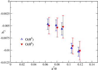
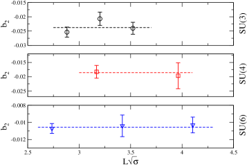
Figure 1: Tests for systematics: (left) dependence of the $SU(6)$ $b_{2}$ results on the truncation adopted in the fitting procedure; (right) dependence of $b_{2}$ on the lattice size adopted (at fixed lattice spacing).

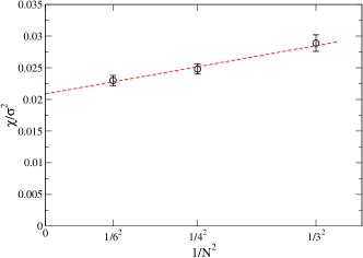
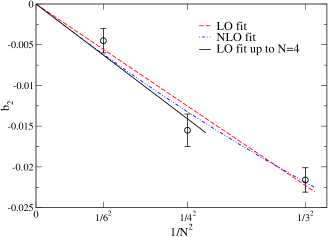
Figure 2: (left) Large $N$ limit of the dimensionless ratio $\chi/\sigma^{2}$; (right) large $N$ limit of $b_{2}$.

As a final application of the imaginary $\theta$ approach, we greatly improved the precision of the $b_{2}$ estimate for $SU(6)$ at finite $T$ presented in [13]: using also data from [6], the final figure of [13] now becomes Fig. 3. With the new, largely reduced, error bars in the low temperature phase, the change of the large $N$ scaling across the transition is now even more evident: for $T<T_{c}$ the large $N$ limit is governed by the same scaling variable $\theta/N$ as at $T=0$, while for $T>T_{c}$ no $N$-dependence is observed in $b_{2}$ and the functional form $\chi(T)(1-\cos(\theta))$ of the $\theta$ dependence (predicted by the dilute instanton gas approximation [3]) is quickly approached. For $T>T_{c}$ Eqs. (3) clearly fails: in the $N\to\infty$ limit $\chi$ vanishes, so there is no reason for $\theta/N$ to be the relevant scaling variable; the study of $b_{2n}$ shows that the correct scaling variable is just $\theta$, suggesting that the theory can be described in terms of effective degrees of freedom carrying an unit of topological charge.

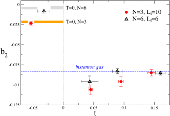
Figure 3: Change of large $N$ scaling for $b_{2}$ across the deconfinement transition, $t=(T-T_{c})/T_{c}$. Updated version of the figure in [13].

4 Conclusions

In this proceeding we reported on the results obtained in the paper [7]: a careful investigation of the $\theta$ dependence of $SU(N)$ gauge theories has been carried out, with the principal aim of studying the deviations from the leading order quadratic behaviour in $\theta$ of the ground state energy density.

In order to carry out such and investigation, the use of simulation performed at imaginary values of the $\theta$ angle was of paramount importance to reduce the statistical errors and the systematics related to finite volume effects. This gave us the possibility of obtaining, for the first time, estimates of $b_{2}$ for $N=4,6$ precise enough to quantitatively verify the large $N$ prediction in Eq. (3). Our final estimates for the coefficients governing the $\theta$ dependence at $T=0$ in the large $N$ limit are:

$$(\chi/\sigma^{2})|_{\infty}=0.0209(11),\quad\bar{b}_{2}=-0.23(3),\quad|\bar{b}_{4}|\lesssim 0.1\ .$$ (10)

Several recent studies (see e.g. [14]) have given new vigor to the idea that confinement is related to semiclasical objects carrying fractional topological charge $1/N$. If the effective interactions between these objects is small enough, one can proceed as in the dilute instanton approximation and obtain for the $\theta$ dependence of the ground state energy density the functional form $E(\theta)-E(0)=\chi(T)(1-\cos(\theta/N))$. This expression correctly reproduce the large $N$ behaviour of Eq. (3) and observed in [5] and [7], however its predictions are not quantitatively accurate: from this functional form, the value $-1/12\simeq-0.0833$ follows for the $\bar{b}_{2}$ coefficients, that is not compatible with the numerical result in Eq. (10). For the case of the $CP^{N-1}$ models, where similar ideas apply and in which the $\bar{b}_{2n}$s are analytically known [7], the situation is even worst: the $\bar{b}_{2n}$s have all the same sign, while the instanton-like expression predicts an alternating series. Whether these discrepancies are due to a different underlying confinement mechanism or to interactions between the effective degrees of freedom is a question that cannot at present be settled and surely deserves further studies.

- [1] E. Vicari and H. Panagopoulos, Phys. Rept. 470, 93 (2009) [arXiv:0803.1593 [hep-th]].
- [2] P. Di Vecchia and G. Veneziano, Nucl. Phys. B 171 (1980) 253.
- [3] D. J. Gross, R. D. Pisarski and L. G. Yaffe, Rev. Mod. Phys. 53, 43 (1981).
- [4] E. Witten, Annals Phys. 128, 363 (1980); E. Witten, Phys. Rev. Lett. 81, 2862 (1998) [hep-th/9807109].
- [5] B. Lucini and M. Teper, JHEP 0106, 050 (2001) [hep-lat/0103027]; L. Del Debbio, H. Panagopoulos and E. Vicari, JHEP 0208, 044 (2002) [hep-th/0204125]; B. Lucini, M. Teper and U. Wenger, Nucl. Phys. B 715, 461 (2005) [hep-lat/0401028].
- [6] C. Bonati, M. D’Elia and A. Scapellato, Phys. Rev. D 93, 025028 (2016) [arXiv:1512.01544 [hep-lat]].
- [7] C. Bonati, M. D’Elia, P. Rossi and E. Vicari, Phys. Rev. D 94, 085017 (2016) [arXiv:1607.06360 [hep-lat]].
- [8] A. Milchev, K. Binder and D. W. Heermann Z. Phys. B -Condensed Matter 63, 521 (1986).
- [9] H. Panagopoulos and E. Vicari, JHEP 1111, 119 (2011) [arXiv:1109.6815 [hep-lat]].
- [10] M. Campostrini, A. Di Giacomo and H. Panagopoulos, Phys. Lett. B 212, 206 (1988).
- [11] B. Berg, Phys. Lett. B 104, 475 (1981); Y. Iwasaki and T. Yoshie, Phys. Lett. B 131, 159 (1983); S. Itoh, Y. Iwasaki and T. Yoshie, Phys. Lett. B 147, 141 (1984); M. Teper, Phys. Lett. B 162, 357 (1985); E. M. Ilgenfritz, M. L. Laursen, G. Schierholz, M. Muller-Preussker and H. Schiller, Nucl. Phys. B 268, 693 (1986).
- [12] C. Bonati and M. D’Elia, Phys. Rev. D 89, 105005 (2014) [arXiv:1401.2441 [hep-lat]]; K. Cichy, A. Dromard, E. Garcia-Ramos, K. Ottnad, C. Urbach, M. Wagner, U. Wenger and F. Zimmermann, PoS LATTICE 2014, 075 (2014) [arXiv:1411.1205 [hep-lat]]; Y. Namekawa, PoS LATTICE 2014, 344 (2015) [arXiv:1501.06295 [hep-lat]]; C. Alexandrou, A. Athenodorou and K. Jansen, Phys. Rev. D 92, 125014 (2015) [arXiv:1509.04259 [hep-lat]]; B. A. Berg and D. A. Clarke, arXiv:1612.07347 [hep-lat].
- [13] C. Bonati, M. D’Elia, H. Panagopoulos and E. Vicari, Phys. Rev. Lett. 110, no. 25, 252003 (2013) [arXiv:1301.7640 [hep-lat]].
- [14] M. Unsal and L. G. Yaffe, Phys. Rev. D 78, 065035 (2008) [arXiv:0803.0344 [hep-th]]; A. Parnachev and A. R. Zhitnitsky, Phys. Rev. D 78, 125002 (2008) [arXiv:0806.1736 [hep-ph]].