Polar Codes and Polar Lattices for the Heegard-Berger Problem

Abstract

Explicit coding schemes are proposed to achieve the rate-distortion function of the Heegard-Berger problem using polar codes. Specifically, a nested polar code construction is employed to achieve the rate-distortion function for the doubly-symmetric binary sources when the side information may be absent. The nested structure contains two optimal polar codes for lossy source coding and channel coding, respectively. Moreover, a similar nested polar lattice construction is employed when the source and the side information are jointly Gaussian. The proposed polar lattice is constructed by nesting a quantization polar lattice and a capacity-achieving polar lattice for the additive white Gaussian noise channel.

I Introduction

The well-known Wyner-Ziv problem is a lossy source coding problem in which a source sequence is to be reconstructed in the presence of correlated side information at the decoder [1]. An interesting question is whether reconstruction with a non-trivial distortion quality can still be obtained in the absence of the side information. The equivalent coding system contains two decoders, one with the side information, and the other without, as shown by Fig. 1.

In 1985, Heegard and Berger [2] characterized the rate-distortion function $R_{HB}\left(D_{1},D_{2}\right)$ for this scenario, where $D_{1}$ is the distortion achieved without side information, $D_{2}$ is the distortion achieved with it, and $R_{HB}\left(D_{1},D_{2}\right)$ denotes the minimum rate required to achieve the distortion pair $\left(D_{1},D_{2}\right)$. They also gave an explicit expression for the quadratic Gaussian case. Kerpez [3] provided upper and lower bounds on the Heegard-Berger rate-distortion function (HBRDF) for the binary case. Later, the explicit expression for $R_{HB}\left(D_{1},D_{2}\right)$ in the binary case was derived in [4] together with the corresponding optimal test channel. Our goal in this paper is to propose explicit coding schemes that can achieve the HBRDF for binary and Gaussian distributions.

The Heegard-Berger problem is a generalization of the classical Wyner-Ziv problem, in which a source sequence is to be reproduced at the decoder within a certain distortion target, and the side information available at the decoder is not available at the encoder. A nested construction of polar codes is presented in [5] to achieve the binary Wyner-Ziv rate-distortion function. For Gaussian sources, a polar lattice to achieve both the standard and Wyner-Ziv rate-distortion functions is proposed in [6]. Different from the solutions of the Wyner-Ziv problem in [5] and [6], we need to consider the requirements for the two decoders jointly. Therefore, we make use of the low-fidelity reconstruction at Decoder 1, and combine it with the original source and the side information to form the nested structure that achieves the optimal distortion for Decoder 2.

The optimality of polar codes for the lossy compression of nonuniform sources is shown in [7]. We employ this scheme as part of our solution, since the optimal forward test channel may be asymmetric in the binary Heegard-Berger problem. Furthermore, it is shown in [8] that polar codes are optimal for general distributed hierarchical source coding problems. The Heegard-Berger problem can also be considered as a successive refinement problem. In this paper, we propose explicit coding schemes using polar codes and polar lattices to achieve the theoretical performance bound in the Heegard-Berger problem. Practical codes for the Gaussian Heegard-Berger problem are also developed in [9] which hybridize trellis and low-density parity-check codes. However, the optimality of this scheme to achieve the HBRDF is not shown in [9].

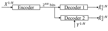
Figure 1: Illustration of the Heegard-Berger rate-distortion problem.

The contributions of this paper can be summarized as follows:

• We propose a nested construction of polar codes for the non-degenerate region of the binary Heegard-Berger problem, and prove that they achieve the HBRDF for doubly symmetric binary sources (DSBS). We consider the reconstruction of the source sequence at Decoder 1, i.e., the decoder without side information, denoted by $\hat{X}_{1}^{1:N}$ and the original source sequence $X^{1:N}$ as a combined source, and further combine this reconstruction $\hat{X}_{1}^{1:N}$ with the original side information $Y^{1:N}$ to obtain a combined side information. By this argument, we obtain another nested construction of polar codes, which achieves the HBRDF of the entire non-degenerate region. In addition, we present an explicit coding scheme by using two-level polar codes to achieve the HBRDF whose forward test channel may be asymmetric. Finally, we prove that polar codes achieve an exponentially decaying block error probability and excess distortion at both decoders for the binary Heegard-Berger problem.

• We then consider the Gaussian Heegard-Berger problem, and propose a polar lattice construction that consists of two nested polar lattices, one of which is additive white Gaussian noise (AWGN) capacity-achieving while the other is Gaussian rate-distortion function achieving. This construction is similar to the one proposed for the Gaussian Wyner-Ziv problem in [6]. However, in the Heegard-Berger problem setting, we need to treat the difference between the original source and its reconstruction at Decoder 1 as a new source, and the difference between the original side information and the reconstruction at Decoder 1 as a new side information. As a result, we can obtain an optimal test channel that connects the new source with the new side information by using additive Gaussian noises. According to this test channel, we can further construct two nested polar lattices that achieve the Gaussian HBRDF of the entire non-degenerate region.

Organization: The paper is organized as follows: Section II presents the background on binary and Gaussian Heegard-Berger problems. The construction of polar codes to achieve the HBRDF for DSBS is investigated in Section III. In Section IV, the polar code construction for the Gaussian Heegard-Berger problem is addressed. The paper is concluded in Section V.

Notation: All random variables are denoted by capital letters, while sets are denoted by capital letters in calligraphic font. $P_{X}$ denotes the probability distribution of a random variable $X$ taking values in set $\mathcal{X}$. For two positive integers $i<j$, $x^{i:j}$ denotes the vector $\left(x^{i},\ldots,x^{j}\right)$, which represents the realizations of random variables $X^{i:j}$. For a set $\mathcal{F}$ of positive integers, $x_{\mathcal{F}}$ denotes the subvector $\{x^{i}\}_{i\in\mathcal{F}}$. For the Gaussian case, we construct polar codes in multiple levels, in which $X_{l}$ denotes a random variable at level $l$, and $x_{l}^{i}$ its $i$-th realization. Then, $x_{l}^{i:j}$ denotes the vector $\left(x_{l}^{i},\ldots,x_{l}^{j}\right)$, and $x_{l}^{\mathcal{F}}$ denotes the subvector $\{x_{l}^{i}\}_{i\in\mathcal{F}}$ at the $l$-th level. $\mathcal{F}^{c}$ and $\left|\mathcal{F}\right|$ denote the complement and cardinality of set $\mathcal{F}$, respectively. For a positive integer $N$, we define $\left[N\right]\triangleq\left\{1,\ldots,N\right\}$. $\boldsymbol{1}\left[x\in\mathcal{X}\right]$ denotes the indicator function, which equals $1$ if $x\in\mathcal{X}$ and $0$ otherwise. Let $I\left(X;Y\right)$ denote the mutual information between $X$ and $Y$. In this paper, all logarithms are base two, and information is measured in bits.

II Problem Statement

II-A Heegard-Berger Problem

Let $\left(\mathcal{X},\mathcal{Y},P_{XY}\right)$ be discrete memoryless sources (DMSs) characterized by the random variables $X$ and $Y$ with a generic joint distribution $P_{XY}$ over the finite alphabets $\mathcal{X}$ and $\mathcal{Y}$.

Definition 1.

An $\left(N,M,D_{1},D_{2}\right)$ Heegard-Berger code for source $X$ with side information $Y$ consists of an encoder $f^{(N)}:\mathcal{X}^{1:N}\rightarrow\left[I_{M}\right]$ and two decoders $g_{1}^{(N)}:\left[I_{M}\right]\rightarrow\mathcal{\hat{X}}_{1}^{1:N}$; $g_{2}^{(N)}:\left[I_{M}\right]\times\mathcal{Y}^{1:N}\rightarrow\mathcal{\hat{X}}_{2}^{1:N}$, where $\mathcal{\hat{X}}_{1},\mathcal{\hat{X}}_{2}$ are finite reconstruction alphabets, such that

$$\mathbb{E}\left[\frac{1}{N}\sum_{j=1}^{N}d\left(X^{j},\hat{X}_{i}^{j}\right)\right] \leq D_{i},\textrm{ }i=1,2,$$

where $\mathbb{E}$ is the expectation operation, and $d\left(\cdot,\cdot\right)<\infty$ is a per-letter distortion measure. In this paper, we set $d\left(\cdot,\cdot\right)$ to be the Hamming distortion for binary sources, and the squared error distortion for Gaussian sources.

Definition 2.

Rate $R$ is said to be $\left\{\left(D_{1},D_{2}\right)-achievable\right\}$, if for every $\epsilon>0$ and sufficiently large $N$ there exists an $\left(N,M,D_{1}+\epsilon,D_{2}+\epsilon\right)$ code with $R+\epsilon\geq\frac{1}{N}\log M$.

The HBRDF, $R_{HB}\left(D_{1},D_{2}\right)$, is defined as the infimum of $\left(D_{1},D_{2}\right)$-achievable rates. A single-letter expression for $R_{HB}\left(D_{1},D_{2}\right)$ is given in the following theorem.

Theorem 3.

([2, Theorem 1])

$$R_{HB}\left(D_{1},D_{2}\right)=\min_{\left(U_{1},U_{2}\right)\in\mathcal{P}\left(D_{1},D_{2}\right)}\left[I\left(X;U_{1}\right)+I\left(X;U_{2}|U_{1},Y\right)\right],$$

where $\mathcal{P}\left(D_{1},D_{2}\right)$ is the set of all auxiliary random variables $\left(U_{1},U_{2}\right)\in\mathcal{U}_{1}\times\mathcal{U}_{2}$ jointly distributed with the generic random variables $\left(X,Y\right)$, such that: i) $Y\leftrightarrow X\leftrightarrow\left(U_{1},U_{2}\right)$ form a Markov chain; ii) $\left|\mathcal{U}_{1}\right|\leq\left|\mathcal{X}\right|+2$ and $\left|\mathcal{U}_{2}\right|\leq\left(\left|\mathcal{X}\right|+1\right)^{2}$; iii) there exist functions $\varphi_{1}$ and $\varphi_{2}$ such that $\mathbb{E}\left[d\left(X,\varphi_{1}\left(U_{1}\right)\right)\right]\leq D_{1}$ and $\mathbb{E}\left[d\left(X,\varphi_{2}\left(U_{1},U_{2},Y\right)\right)\right]\leq D_{2}.$

II-B Doubly Symmetric Binary Sources

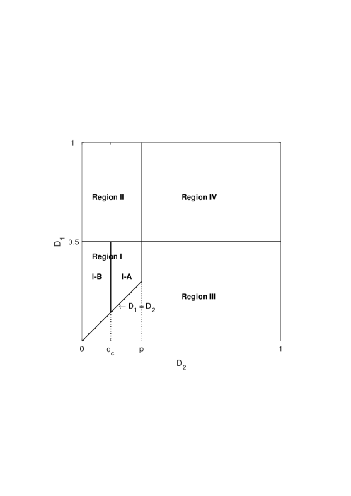
Figure 2: Illustration of the HBRDF regions for DSBS, where $d_{c}$ is the critical distortion.

Let $X$ be a binary DMS, i.e., $\mathcal{X}=\left\{0,1\right\}$, with uniform distribution. The binary side information is specified by $Y=X\oplus Z$, where $Z$ is an independent Bernoulli random variable with $P_{Z}\left(z=1\right)=p<0.5$, and $\oplus$ denotes modulo two addition.

The HBRDF for DSBS can be characterized over four regions [3]. Region I ($0\leq D_{1}<0.5$ and $0\leq D_{2}<\min\left(D_{1},p\right)$) is a non-degenerate region, and $R_{HB}(D_{1},D_{2})$ is a function of $D_{1}$ and $D_{2}$; Region II ($D_{1}\geq 0.5$ and $0\leq D_{2}\leq p$) is a degenerate region as the Heegard-Berger problem boils down to the Wyner-Ziv problem for the second decoder; Region III ($0\leq D_{1}\leq 0.5$ and $D_{2}\geq\min\left(D_{1},p\right)$) is also degenerate since the problem boils down to the standard lossy compression problem for the first decoder; Region IV ($D_{1}>0.5$ and $D_{2}>p$) can be trivially achieved without coding. These four regions are depicted in Fig. 2. Note that, the HBRDF in the degenerate Regions II and III can be achieved by using polar codes as described in [5]. Here we focus on the non-degenerate Region I.

The explicit calculation of HBRDF for DSBS in Region I is given in [4] as follows:

Define the function

$$S_{D_{1}}\left(\alpha,\mu,\theta,\theta_{1}\right)\triangleq 1-h\left(D_{1}*p\right)+\left(\theta-\theta_{1}\right)G\left(\alpha\right)+\theta_{1}G\left(\mu\right)+\left(1-\theta\right)G\left(\gamma\right),$$

where

$$\begin{array}[]{cc}\gamma\triangleq&\begin{cases}\frac{D_{1}-\left(\theta-\theta_{1}\right)\left(1-\alpha\right)-\theta_{1}\mathbf{\mu}}{1-\theta}&\theta\neq 1\\ 0.5&\theta=1\end{cases}\end{array},$$

on the domain $0\leq\theta_{1}\leq\theta\leq 1,\textrm{ }0\leq\alpha,\mu\leq p,\textrm{ }p\leq\gamma\leq 1-p.$

The following theorem characterizes the HBRDF in Region I.

Theorem 4.

[4, Theorem 2] For $0\leq D_{1}<0.5$ and $0\leq D_{2}<\min\left(D_{1},p\right)$, we have $R_{HB}\left(D_{1},D_{2}\right)=\min S_{D_{1}}\left(\alpha,\mu,\theta,\theta_{1}\right)$, where the minimization is over all $\theta_{1}$, $\theta$, $\alpha$ and $\mu$ variables that satisfy $0\leq\theta_{1}\leq\theta\leq 1$, $0\leq\alpha,\mu\leq p$ and $\left(\theta-\theta_{1}\right)\alpha+\theta_{1}\mu+\left(1-\theta\right)p=D_{2}$.

The corresponding forward test channel structure is also given in [4], reproduced in Table I. It constructs random variables with joint distribution $P_{X,U_{1},U_{2}}\left(x,u_{1},u_{2}\right)$, which satisfy $I\left(X;U_{1}\right)+I\left(X;U_{2}|U_{1},Y\right)=S_{D_{1}}\left(\alpha,\mu,\theta,\theta_{1}\right)$.

	$\left(u_{1},x\right)=(0,0)$	$\left(u_{1},x\right)=(0,1)$	$\left(u_{1},x\right)=(1,0)$	$\left(u_{1},x\right)=(1,1)$
$u_{2}=0$	$\frac{1}{2}\theta_{1}\left(1-\mu\right)$	$\frac{1}{2}\theta_{1}\mu$	$\frac{1}{2}\left(\theta-\theta_{1}\right)\left(1-\alpha\right)$	$\frac{1}{2}\left(\theta-\theta_{1}\right)\alpha$
$u_{2}=1$	$\frac{1}{2}\left(\theta-\theta_{1}\right)\alpha$	$\frac{1}{2}\left(\theta-\theta_{1}\right)\left(1-\alpha\right)$	$\frac{1}{2}\theta_{1}\mu$	$\frac{1}{2}\theta_{1}\left(1-\mu\right)$
$u_{2}=2$	$\frac{1}{2}\left(1-\theta\right)\left(1-\gamma\right)$	$\frac{1}{2}\left(1-\theta\right)\gamma$	$\frac{1}{2}\left(1-\theta\right)\gamma$	$\frac{1}{2}\left(1-\theta\right)\left(1-\gamma\right)$

Table I: Joint distribution $P_{X,U_{1},U_{2}}\left(x,u_{1},u_{2}\right)$ [4].

Next, we recall the function $G\left(u\right)\triangleq h\left(p*u\right)-h(u)$ from [1], defined over the domain $0\leq u\leq 1$, where $h(u)$ is the binary entropy function $h(u)\triangleq-u\log u-(1-u)\log\left(1-u\right)$, and $p*u$ is the binary convolution for $0\leq p,u\leq 1$, defined as $p*u\triangleq p\left(1-u\right)+u\left(1-p\right)$. Then, recall the definition of the critical distortion, $d_{c}$, in the Wyner-Ziv problem for DSBS [1], for which $\frac{G\left(d_{c}\right)}{d_{c}-p}=G^{\prime}\left(d_{c}\right)$.

The following corollary from [4] specifies an explicit the characterization of HBRDF for DSBS in Region I-B in Fig. 2 specified by $D_{2}\leq\min\left(d_{c},D_{1}\right)$ and $D_{1}\leq 0.5$.

Corollary 5.

([4, Corollary 2]) For distortion pairs $\left(D_{1},D_{2}\right)$ satisfying $D_{1}\leq 0.5$ and $D_{2}\leq\min\left(d_{c},D_{1}\right)$ (i.e., Region I-B in Fig. 2), we have

$$R_{HB}\left(D_{1},D_{2}\right)=1-h\left(D_{1}*p\right)+G\left(D_{2}\right).$$ (1)

From [4], the optimal forward test channel for Region I-B is given as a cascade of two binary symmetric channels (BSCs), as depicted in Fig. 3.

In Section III, we first propose a polar code design that achieves the HBRDF in Region I-B for DSBSs. We then provide a general polar code construction achieving the HBRDF in the entire Region I.

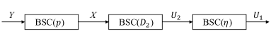
Figure 3: The optimal forward test channel for Region I-B. The crossover probability $\eta$ for the BSC between $U_{2}$ and $U_{1}$ satisfies $D_{2}*\eta=D_{1}$.

II-C Gaussian Sources

Suppose $Y=X+Z$, where $X$ and $Z$ are independent (zero-mean) Gaussian random variables with variances $\sigma_{X}^{2}$ and $\sigma_{Z}^{2}$, respectively, i.e., $X\sim\mathcal{N}\left(0,\sigma_{X}^{2}\right)$ and $Z\sim\mathcal{N}\left(0,\sigma_{Z}^{2}\right)$. The explicit expression for $R_{HB}\left(D_{1},D_{2}\right)$ in this case is given in [2]. The optimal test channels are given by $X=U_{1}+Z_{1}$ and $X=U_{2}+Z_{2}$, where $Z$, $Z_{1}$ and $Z_{2}$ are independent zero-mean Gaussian random variables. We have $Z_{i}\sim\mathcal{N}\left(0,D_{i}\right),\textrm{ }i=1,2$.

For $D_{1}\leq\sigma_{X}^{2}$ and $D_{2}\geq\frac{D_{1}\sigma_{Z}^{2}}{D_{1}+\sigma_{Z}^{2}}$, the problem degenerates into a classical lossy compression problem for Decoder 1, and the HBRDF is given by $R_{HB}\left(D_{1},D_{2}\right)=\frac{1}{2}\log\left(\frac{\sigma_{X}^{2}}{D_{1}}\right)$. For $D_{1}>\sigma_{X}^{2}$ and $D_{2}\leq\frac{D_{1}\sigma_{Z}^{2}}{D_{1}+\sigma_{Z}^{2}}$, the problem degenerates into a Wyner-Ziv coding problem for Decoder 2, and we have $R_{HB}\left(D_{1},D_{2}\right)=\frac{1}{2}\log\left(\frac{\sigma_{X}^{2}\sigma_{Z}^{2}}{D_{2}\left(\sigma_{X}^{2}+\sigma_{Z}^{2}\right)}\right)$. The region specified by $D_{1}>\sigma_{X}^{2}$ and $D_{2}\geq\frac{D_{1}\sigma_{Z}^{2}}{D_{1}+\sigma_{Z}^{2}}$ requires no coding. Polar lattice codes that meet the classical and Wyner-Ziv rate-distortion functions for Gaussian sources, introduced in [6], can be used to achieve the HBRDF in these degenerate regions. The only non-degenerate distortion region is specified by $D_{1}\leq\sigma_{X}^{2}$ and $D_{2}\leq\frac{D_{1}\sigma_{Z}^{2}}{D_{1}+\sigma_{Z}^{2}}$, and the HBRDF in this region is given by [2]:

$$R_{HB}\left(D_{1},D_{2}\right)=\frac{1}{2}\log\left(\frac{\sigma_{X}^{2}\sigma_{Z}^{2}}{D_{2}\left(D_{1}+\sigma_{Z}^{2}\right)}\right).$$ (2)

We will focus on the construction of polar lattice codes that achieve the HBRDF in (2) in Section IV.

III Polar Codes for DSBS

In this section, we present a construction of polar codes that achieves $R_{HB}\left(D_{1},D_{2}\right)$ for DSBS in Region I. First, we give a brief overview of polar codes.

Let $G_{2}\triangleq\left[\begin{smallmatrix}1&0\\ 1&1\end{smallmatrix}\right]$, and define $G_{N}\triangleq G_{2}^{\otimes n}$ as the generator matrix of polar codes with length $N=2^{n}$, where ‘$\otimes$’ denotes the Kronecker product. A polar code $\mathcal{C}_{N}\left(\mathcal{F},u_{\mathcal{F}}\right)$ [5] is a linear code defined by $\mathcal{C}_{N}\left(\mathcal{F},u_{\mathcal{F}}\right)=\left\{v^{1:N}G_{N}:v_{\mathcal{F}}=u_{\mathcal{F}},v_{\mathcal{F}^{c}}\in\left\{0,1\right\}^{\left|\mathcal{F}^{c}\right|}\right\},$ for any $\mathcal{F}\subseteq\left[N\right]$ and $u_{\mathcal{F}}\in\left\{0,1\right\}^{\left|\mathcal{F}\right|}$, where $\mathcal{F}$ is referred to as the frozen set. The code $\mathcal{C}_{N}\left(\mathcal{F},u_{\mathcal{F}}\right)$ is constructed by fixing $u_{\mathcal{F}}$ and varying the values in $\mathcal{F}^{c}$. Moreover, the frozen set can be determined by the Bhattacharyya parameter [5]. For a binary memoryless asymmetric channel with input $X\in\mathcal{X}=\left\{0,1\right\}$ and output $Y\in\mathcal{Y}$, the Bhattacharyya parameter $Z$ is defined as $Z\left(X|Y\right)\triangleq 2\sum_{y}\sqrt{P_{X,Y}\left(0,y\right)P_{X,Y}\left(1,y\right)}$.

III-A Polar Code Construction for Region I-B

We observe from the proof of Theorem 4 in [4] that the auxiliary random variable $U_{1}$ can be considered as the output of a BSC with crossover probability $D_{1}$ and input $X$. Therefore, as for Region I-B, the minimum rate for Decoder 1 to achieve the target distortion $D_{1}$ is $R_{1}=I\left(U_{1};X\right)=1-h\left(D_{1}\right).$ It is shown in [10, Theorem 3] that polar codes can achieve the rate-distortion function of binary symmetric sources. An explicit code construction is also provided in [10]. Considering the source sequence $X^{1:N}$ as $N$ independent and identically distributed (i.i.d) copies of $X$, we know from [10, Theorem 3] that Decoder 1 can recover a reconstruction $\hat{X}_{1}^{1:N}$ that is asymptotically close to $U_{1}^{1:N}$ as $N$ becomes sufficiently large. Therefore, we assume that both Decoder 1 and Decoder 2 can obtain $U_{1}^{1:N}$ in the following.

Decoder 2 observes the side information $Y^{1:N}$, in addition to $U_{1}^{1:N}$ that can be reconstructed using the same method as Decoder 1. Hence, both $Y^{1:N}$ and $U_{1}^{1:N}$ can be considered as side information for Decoder 2 to achieve distortion $D_{2}$. Therefore, the problem at Decoder 2 is very similar to Wyner-Ziv coding except that the decoder observes extra side information.

Recall that achieving the Wyner-Ziv rate-distortion function using polar codes is based on the nested code structure proposed in [5]. Consider the Wyner-Ziv problem consisting of compressing a source $X^{1:N}$ in the presence of correlated side information $Y^{1:N}$ using polar codes, where $X$ and $Y$ are DSBS. The code $\mathcal{C}_{s}$ with corresponding frozen set $\mathcal{F}_{s}$ is designed to be a good source code for distortion $D_{2}$. Further, the code $\mathcal{C}_{c}$ with corresponding frozen set $\mathcal{F}_{c}$ is designed to be a good channel code for BSC$\left(D_{2}*p\right)$. It has been shown in [5] that $\mathcal{F}_{c}\supseteq\mathcal{F}_{s}$, because the test channel BSC$\left(D_{2}*p\right)$ is degraded with respect to BSC$\left(D_{2}\right)$. In this case, the encoder transmits to the decoder the sub-vector that belongs to the index set $\mathcal{F}_{c}$\$\mathcal{F}_{s}$. The optimality of this scheme is proven in [5].

Similarly, the optimal rate-distortion performance for Decoder 2 in the Heegard-Berger problem can also be achieved by using nested polar codes. For $\left(U_{1},U_{2}\right)\in\mathcal{P}\left(D_{1},D_{2}\right)$, we have

$$I\left(X;U_{2}|U_{1},Y\right) =I\left(U_{2};X,U_{1},Y\right)-I\left(U_{2};Y,U_{1}\right)$$ (3)

$$=I\left(U_{2};X,U_{1}\right)-I\left(U_{2};Y,U_{1}\right).$$

The second equality holds since $Y\leftrightarrow X\leftrightarrow\left(U_{1},U_{2}\right)$ form a Markov chain. Motivated by $\left(\ref{eq:rate of decoder 2 binary}\right)$, the code $\mathcal{C}_{s_{2}}$ with corresponding frozen set $\mathcal{F}_{s_{2}}$ is designed to be a good source code for the source pair $\left(X^{1:N},U_{1}^{1:N}\right)$ with reconstruction $U_{2}^{1:N}$. $T_{s}$ denotes the test channel for this source code. Additionally, the code $\mathcal{C}_{c_{2}}$ with corresponding frozen set $\mathcal{F}_{c_{2}}$ is designed to be a good channel code for the test channel $T_{c}$ with input $U_{2}^{1:N}$ and output $\left(Y^{1:N},U_{1}^{1:N}\right)$. According to [5, Lemma 4.7], in order to show the nested structure between $\mathcal{C}_{s_{2}}$ and $\mathcal{C}_{c_{2}}$, it is sufficient to show that $T_{c}$ is stochastically degraded with respect to $T_{s}$.

Definition 6.

(Channel Degradation [5]). Let $T_{1}:\mathcal{U}\rightarrow\mathcal{Y}$ and $T_{2}:\mathcal{U}\rightarrow\mathcal{X}$ be two binary discrete memoryless channels. We say that $T_{1}$ is stochastically degraded with respect to $T_{2}$, if there exists a discrete memoryless channel $T:\mathcal{X}\rightarrow\mathcal{Y}$ such that

$$P_{Y|U}(y|u)=\sum_{x\in\mathcal{X}}P_{X|U}(x|u)P_{Y|X}(y|x).$$

Proposition 7.

$T_{c}:U_{2}\rightarrow\left(Y,U_{1}\right)$ is stochastically degraded with respect to $T_{s}:U_{2}\rightarrow\left(X,U_{1}\right)$, if the random variables $\left(X,Y,U_{1},U_{2}\right)$ agree with the forward test channel as shown in Fig. 3.

Proof:

From the test channel structure in Fig. 3, $Y\leftrightarrow X\leftrightarrow U_{2}\leftrightarrow U_{1}$ form a Markov chain. By definition, we have $P_{X,U_{1}|U_{2}}\left(x,u_{1}|u_{2}\right)=P_{X|U_{2}}\left(x|u_{2}\right)P_{U_{1}|U_{2}}\left(u_{1}|u_{2}\right).$ We also have

$$P_{Y,U_{1}|U_{2}}\left(y,u_{1}|u_{2}\right) =P_{Y|U_{2}}\left(y|u_{2}\right)P_{U_{1}|U_{2}}\left(u_{1}|u_{2}\right)$$

$$=\sum_{x}P_{X,Y|U_{2}}\left(x,y|u_{2}\right)P_{U_{1}|U_{2}}\left(u_{1}|u_{2}\right)$$

$$=\sum_{x}P_{X|U_{2}}\left(x|u_{2}\right)P_{Y|X,U_{2}}\left(y|x,u_{2}\right)P_{U_{1}|U_{2}}\left(u_{1}|u_{2}\right)$$

$$=\sum_{x}P_{X,U_{1}|U_{2}}\left(x,u_{1}|u_{2}\right)P_{Y|X}\left(y|x\right),$$

completing the proof. ∎

Therefore, we can claim that $\mathcal{F}_{c_{2}}\supseteq\mathcal{F}_{s_{2}}$ by [5, Lemma 4.7], and rather than sending the entire vector that belongs to the index set $\mathcal{F}_{s_{2}}^{c}$, the encoder sends only the sub-vector that belongs to $\mathcal{F}_{c_{2}}$\$\mathcal{F}_{s_{2}}$ to Decoder 2, since Decoder 2 can extract some information on $U_{2}^{1:N}$ from the available side information $\left(U_{1}^{1:N},Y^{1:N}\right)$. As a result, the polar code construction for the Heegard-Berger problem in Region I-B is given as follows:

Encoding: The encoder first applies lossy compression to source sequence $X^{1:N}$ with reconstruction $U_{1}^{1:N}$ and corresponding average distortion $D_{1}$. We construct the code $\mathcal{C}_{s_{1}}=\mathcal{C}_{N}\left(\mathcal{F}_{s_{1}},\bar{0}\right)=\left\{w^{1:N}G_{N}:w_{\mathcal{F}_{s_{1}}}=\bar{0},w_{\mathcal{F}_{s_{1}}^{c}}\in\left\{0,1\right\}^{\left|\mathcal{F}_{s_{1}}^{c}\right|}\right\}$, and the encoder transmits the compressed sequence $w_{\mathcal{F}_{s_{1}}^{c}}$ to the decoders. The encoder is also able to recover $U_{1}^{1:N}$ from $\mathcal{C}_{s_{1}}$. Next, the encoder applies lossy compression jointly for sources $\left(X^{1:N},U_{1}^{1:N}\right)$ with reconstruction $U_{2}^{1:N}$ and target distortion $D_{2}$ and $d\left(U_{1},U_{2}\right)=\eta$. We then construct $\mathcal{C}_{s_{2}}=\mathcal{C}_{N}\left(\mathcal{F}_{s_{2}},\bar{0}\right)$. Finally, the encoder applies channel coding to the symmetric test channel $T_{c}$ with input $U_{2}^{1:N}$ and output $\left(Y^{1:N},U_{1}^{1:N}\right)$. We derive $\mathcal{C}_{c_{2}}=\mathcal{C}_{N}\left(\mathcal{F}_{c_{2}},u_{\mathcal{F}_{c_{2}}}\left(\bar{v}\right)\right)$, where $u_{\mathcal{F}_{c_{2}}}\left(\bar{v}\right)$ is defined by $u_{\mathcal{F}_{s_{2}}}=\bar{0}$ and $u_{\mathcal{F}_{c_{2}}\backslash\mathcal{F}_{s_{2}}}=\bar{v}$ for $\bar{v}\in\{0,1\}^{\left|\mathcal{F}_{c_{2}}\backslash\mathcal{F}_{s_{2}}\right|}$. The encoder sends the sub-vector $u_{\mathcal{F}_{c_{2}}\backslash\mathcal{F}_{s_{2}}}$ to the decoders.

Decoding: Decoder 1 receives $w_{\mathcal{F}_{s_{1}}^{c}}$ and outputs the reconstruction sequence $u_{1}^{1:N}=w^{1:N}G_{N}$. Decoder 2 receives $u_{\mathcal{F}_{c_{2}}\backslash\mathcal{F}_{s_{2}}}$, and hence, it can derive $u_{\mathcal{F}_{c_{2}}}$. Moreover, Decoder 2 can also recover $U_{1}^{1:N}$ from $w_{\mathcal{F}_{s_{1}}^{c}}$. Decoder 2 applies the successive cancellation (SC) decoding algorithm to obtain the codeword $U_{2}^{1:N}$ from the realizations of $\left(Y^{1:N},U_{1}^{1:N}\right)$.

Next we present the rates that can be achieved by the proposed scheme. From the polarization theorem for lossy source coding in [10], we know that reliable decoding at Decoder 1 will be achieved with high probability if $\frac{\left|\mathcal{F}_{s_{1}}^{c}\right|}{N}\xrightarrow{N\rightarrow\infty}I\left(U_{1};X\right)=1-h\left(D_{1}\right)$.

From the polarization theorems for source and channel coding [5], the code rate required for reliable decoding at Decoder 2 can be derived by

$$\frac{\left|\mathcal{F}_{c_{2}}\right|-\left|\mathcal{F}_{s_{2}}\right|}{N}\xrightarrow{N\rightarrow\infty} I\left(U_{2};X,U_{1}\right)-I\left(U_{2};Y,U_{1}\right)$$

$$=I\left(U_{2};X\right)+I\left(U_{1};X,U_{2}\right)-I\left(U_{1};X\right)-I\left(U_{2};Y\right)-I\left(U_{1};Y,U_{2}\right)+I\left(U_{1};Y\right)$$

$$=G\left(D_{2}\right)-G\left(D_{1}\right).\text{}$$

Therefore, the total rate will be asymptotically given by $\frac{\left|\mathcal{F}_{s_{1}}^{c}\right|+\left|\mathcal{F}_{c_{2}}\right|-\left|\mathcal{F}_{s_{2}}\right|}{N}\xrightarrow{N\rightarrow\infty}1-h\left(D_{1}*p\right)+G\left(D_{2}\right),$ for Region I-B.

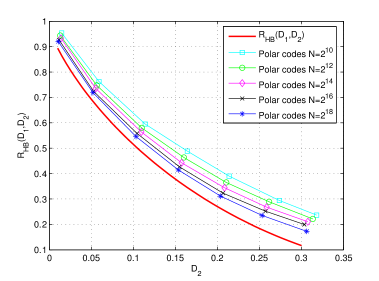
Figure 4: Simulation performance of $R_{HB}\left(D_{1},D_{2}\right)$ corresponding to $D_{2}$ for Region I-B.

Furthermore, according to [5, 10], the expected distortions asymptotically approach the target values $D_{1}$ and $D_{2}$ at Decoders 1 and 2, respectively, as $N$ becomes sufficiently large. The encoding and decoding complexity of this scheme is $O\left(N\log N\right)$.

Note that, in our scheme, the performance of Decoder 2 is more challenging than that of Decoder 1. Thus, the simulation is conducted by fixing $D_{1}=0.35$, $p=0.4$, and varying $D_{2}\in\left(0,\min\left(d_{c},D_{1}\right)\right)$. These settings satisfy the requirements for Region I-B. The performance curves are shown in Fig. 4 for $n=10,12,14,16,18$. It shows that the performances achieved by polar codes approaches the HBRDF as $n$ increases.

III-B Coding Scheme for Entire Region I

As Theorem 4 defines the $R_{HB}\left(D_{1},D_{2}\right)$ for the entire Region I, we now present a coding scheme that can achieve the HBRDF for the entire Region I. Note that $R_{HB}\left(D_{1},D_{2}\right)$ of Region I-B can be explicitly calculated by Corollary 5. Therefore, we can also achieve Region I-B straightforwardly as shown in Section III-A.

From the optimal test channel structure shown in Table I, $U_{2}$ is a ternary random variable, i.e., $\mathcal{U}_{2}=\left\{0,1,2\right\}$. Therefore, we express $U_{2}$ as two binary random variables $U_{a}$ and $U_{b}$, where $U_{2}=2U_{b}+U_{a}$, i.e., $\left(U_{a},U_{b}\right)\in\left\{00,10,01\right\}$. For Decoder 1, we can apply the same scheme specified in the previous subsection to achieve $D_{1}$. Again, $U_{1}^{1:N}$ and $Y^{1:N}$ can be considered as side information for Decoder 2. Then, the rate required to transmit $U_{2}^{1:N}$ is evaluated as $I\left(X;U_{2}|U_{1},Y\right)=I\left(X;U_{a},U_{b}|U_{1},Y\right)=I\left(X;U_{a}|U_{1},Y\right)+I\left(X;U_{b}|U_{1},U_{a},Y\right)$. Accordingly we can design two separate coding schemes to achieve the rates $I\left(X;U_{a}|U_{1},Y\right)$ and $I\left(X;U_{b}|U_{1},U_{a},Y\right)$, respectively.

Since $Y\leftrightarrow X\leftrightarrow(U_{1},U_{a},U_{b})$ form a Markov chain, we have $I\left(X;U_{a}|U_{1},Y\right)=I\left(U_{a};X,U_{1}\right)-I\left(U_{a};Y,U_{1}\right)$, and the test channel $T_{C_{a}}:U_{a}\rightarrow\left(Y,U_{1}\right)$ is degraded with respect to $T_{S_{a}}:U_{a}\rightarrow\left(X,U_{1}\right)$. We can observe from Table I that $U_{a}$ and $U_{b}$ can be nonuniform.

Let $K^{1:N}=U_{a}^{1:N}G_{N}$, and for $0<\beta<0.5$, the frozen set $\mathcal{F}_{S_{a}}\left(\mathcal{F}_{C_{a}}\right)$, the information set $\mathcal{I}_{S_{a}}\left(\mathcal{I}_{C_{a}}\right)$, and the shaping set $\mathcal{S}_{S_{a}}\left(\mathcal{S}_{C_{a}}\right)$ can be identified as

$$\begin{split}&\mathcal{F}_{S_{a}}=\left\{i\in[N]:Z\left(K^{i}|K^{1:i-1},X^{1:N},U_{1}^{1:N}\right)\geq 1-2^{-N^{\beta}}\right\}\\ &\mathcal{I}_{S_{a}}=\left\{i\in[N]:Z\left(K^{i}|K^{1:i-1},X^{1:N},U_{1}^{1:N}\right)<1-2^{-N^{\beta}}\right\}\cap\left\{i\in[N]:Z\left(K^{i}|K^{1:i-1}\right)>2^{-N^{\beta}}\right\}\\ &\mathcal{S}_{S_{a}}=\left\{i\in[N]:Z\left(K^{i}|K^{1:i-1}\right)\leq 2^{-N^{\beta}}\right\},\\ &\mathcal{F}_{C_{a}}=\left\{i\in[N]:Z\left(K^{i}|K^{1:i-1},Y^{1:N},U_{1}^{1:N}\right)\geq 1-2^{-N^{\beta}}\right\}\\ &\mathcal{I}_{C_{a}}=\left\{i\in[N]:Z\left(K^{i}|K^{1:i-1},Y^{1:N},U_{1}^{1:N}\right)\leq 2^{-N^{\beta}}\right\}\cap\left\{i\in[N]:Z\left(K^{i}|K^{1:i-1}\right)\geq 1-2^{-N^{\beta}}\right\}\\ &\mathcal{S}_{C_{a}}=\left\{i\in[N]:Z\left(K^{i}|K^{1:i-1}\right)<1-2^{-N^{\beta}}\right\}\\ &\hskip 40.15pt\cup\left\{i\in[N]:\textrm{ }2^{-N^{\beta}}<Z\left(K^{i}|K^{1:i-1},Y^{1:N},U_{1}^{1:N}\right)<1-2^{-N^{\beta}}\right\}.\end{split}$$ (4)

By [5, Lemma 4.7] and channel degradation, we have $\mathcal{F}_{S_{a}}\subseteq\mathcal{F}_{C_{a}}$, $\mathcal{I}_{C_{a}}\subseteq\mathcal{I}_{S_{a}}$ and $\mathcal{S}_{S_{a}}\subseteq\mathcal{S}_{C_{a}}$. In addition, we observe that $\mathcal{S}_{C_{a}}\backslash\mathcal{S}_{S_{a}}$ can be written as

$$\mathcal{S}_{C_{a}}\backslash\mathcal{S}_{S_{a}}= \left\{i\in[N]:2^{-N^{\beta}}<Z\left(K^{i}|K^{1:i-1}\right)<1-2^{-N^{\beta}}\right\}\cup$$

$$\left\{i\in[N]:\textrm{ }2^{-N^{\beta}}<Z\left(K^{i}|K^{1:i-1},Y^{1:N},U_{1}^{1:N}\right)<1-2^{-N^{\beta}}\right\},$$

therefore, the proportion $\frac{\left|\mathcal{S}_{C_{a}}\backslash\mathcal{S}_{S_{a}}\right|}{N}\rightarrow 0$, as $N\rightarrow\infty$.

Encoding: The encoder first applies lossy compression to $X^{1:N}$ with target distortion $D_{1}$ to obtain $U_{1}^{1:N}$, and treats $\left(X^{1:N},U_{1}^{1:N}\right)$ as a joint source sequence to evaluate $K_{\mathcal{I}_{S_{a}}}$ by randomized rounding with respect to $P_{K^{i}|K^{1:i-1},X^{1:N},U_{1}^{1:N}}$, i.e.,

$$k^{i}=\begin{cases}0&\textrm{w.p. }P_{K^{i}|K^{1:i-1},X^{1:N},U_{1}^{1:N}}\left(0|k^{1:i-1},x^{1:N},u_{1}^{1:N}\right)\\ 1&\textrm{w.p. }P_{K^{i}|K^{1:i-1},X^{1:N},U_{1}^{1:N}}\left(1|k^{1:i-1},x^{1:N},u_{1}^{1:N}\right)\end{cases}\textrm{if }i\in\mathcal{I}_{S_{a}}$$ (5)

and

$$k^{i}=\begin{cases}\tilde{k}^{i}&\textrm{if }i\in\mathcal{F}_{S_{a}}\\ \arg\max_{k}P_{K^{i}|K^{1:i-1}}\left(k|k^{1:i-1}\right)&\textrm{if }i\in\mathcal{S}_{S_{a}},\end{cases}$$ (6)

where ‘w.p.’ is an abbreviation of ‘with probability’ in (5), and $\tilde{k}^{i}$ is chosen uniformly from $\left\{0,1\right\}$ and shared between the encoder and the decoders before lossy compression. Also note that the second formula in (6) is in fact the maximum a posteriori (MAP) decision for $i\in\mathcal{S}_{S_{a}}$. The encoder sends $K_{\mathcal{I}_{S_{a}}\backslash\mathcal{I}_{C_{a}}}$ to the decoders.

Decoding: Using the pre-shared $K_{\mathcal{F}_{S_{a}}}$ and received $K_{\mathcal{I}_{S_{a}}\backslash\mathcal{I}_{C_{a}}}$, Decoder 2 recovers $K_{\mathcal{I}_{C_{a}}}$ and $K_{\mathcal{S}_{S_{a}}}$ from the side information sequences $Y^{1:N}$ and $U_{1}^{1:N}$ by SC decoding algorithm and the MAP rule, respectively. Hence we obtain $K^{1:N}$. $K_{\mathcal{I}_{C_{a}}\cup\mathcal{S}_{S_{a}}}$ and $K_{\mathcal{S}_{C_{a}}\backslash\mathcal{S}_{S_{a}}}$ can be recovered with vanishing error probability, since their Bhattacharyya parameters are arbitrarily small when $N\rightarrow\infty$. Therefore, the reconstruction is given by $U_{a}^{1:N}=K^{1:N}G_{N}$.

Theorem 8.

[6, Theorem 2] Let $Q_{K^{1:N},X^{1:N},U_{1}^{1:N}}$ denote the resulting joint distribution derived from (5) and (6). Let $P_{K^{1:N},X^{1:N},U_{1}^{1:N}}$ denote the joint distribution as a result of another encoder that uses (5) for $i\in\left[N\right]$. For any $\beta^{\prime}<\beta<0.5$ satisfying (4) and $R_{a}=\frac{\left|\mathcal{I}_{S_{a}}\backslash\mathcal{I}_{C_{a}}\right|}{N}>I\left(X;U_{a}|U_{1},Y\right)$, we have

$$\mathbb{V}\left(P_{K^{1:N},X^{1:N},U_{1}^{1:N}},Q_{K^{1:N},X^{1:N},U_{1}^{1:N}}\right)=O\left(2^{-N^{\beta^{\prime}}}\right),$$ (7)

where $\mathbb{V}(P_{X},Q_{X})\triangleq\frac{1}{2}\sum_{x}\left|P_{X}(x)-Q_{X}(x)\right|$ denotes the variational distance between distributions $P_{X}$ and $Q_{X}$.

Note that, from [7], $K_{\mathcal{S}_{C_{a}}}$ should be covered by a pre-shared random mapping to achieve (7). However, it is shown in [6, Theorem 2] that replacing the random mapping with MAP decision for $K_{\mathcal{S}_{S_{a}}}$ preserves the optimality. Thus, we utilize MAP decoder if $i\in\mathcal{S}_{S_{a}}$ in our scheme.

In terms of the second level, the encoder and Decoder 2 first recover $U_{a}^{1:N}$. Consequently, the encoder treats $\left(X^{1:N},U_{1}^{1:N},U_{a}^{1:N}\right)$ as a joint source, and Decoder 2 treats $\left(Y^{1:N},U_{1}^{1:N},U_{a}^{1:N}\right)$ as a joint side information. Likewise, according to $Y\leftrightarrow X\leftrightarrow(U_{1},U_{a},U_{b})$, we have $I\left(X;U_{b}|U_{1},U_{a},Y\right)=I\left(U_{b};X,U_{1},U_{a}\right)-I\left(U_{b};Y,U_{1},U_{a}\right)$ and the test channel $T_{C_{b}}:U_{b}\rightarrow\left(Y,U_{1},U_{a}\right)$ is degraded with respect to $T_{S_{b}}:U_{b}\rightarrow\left(X,U_{1},U_{a}\right)$.

Similar to the first level, let $W^{1:N}=U_{b}^{1:N}G_{N}$ and the frozen set $\mathcal{F}_{S_{b}}\left(\mathcal{F}_{C_{b}}\right)$, the information set $\mathcal{I}_{S_{b}}\left(\mathcal{I}_{C_{b}}\right)$, and the shaping set $\mathcal{S}_{S_{b}}\left(\mathcal{S}_{C_{b}}\right)$ can be adopted from (4) by replacing $K$, $\left(X,U_{1}\right)$ and $\left(Y,U_{1}\right)$ with $W$, $\left(X,U_{1},U_{a}\right)$ and $\left(Y,U_{1},U_{a}\right)$, respectively. As a result, we have $\mathcal{F}_{S_{b}}\subseteq\mathcal{F}_{C_{b}}$, $\mathcal{I}_{C_{b}}\subseteq\mathcal{I}_{S_{b}}$ and $\mathcal{S}_{S_{b}}\subseteq\mathcal{S}_{C_{b}}$ by [5, Lemma 4.7] and channel degradation. The encoder evaluates $W_{\mathcal{I}_{S_{b}}}$ by randomized rounding with respect to $P_{W^{i}|W^{1:i-1},X^{1:N},U_{1}^{1:N},U_{a}^{1:N}}$, $W_{\mathcal{F}_{S_{b}}}$ are pre-shared random bits uniformly chosen from $\left\{0,1\right\}$, and $W_{\mathcal{S}_{S_{b}}}$ is determined by MAP decoder defined as $\arg\max_{w}P_{W^{i}|W^{1:i-1}}\left(w|w^{1:i-1}\right)$. The encoder sends $W_{\mathcal{I}_{S_{b}}\backslash\mathcal{I}_{C_{b}}}$ to the decoders. Decoder 2 recovers $W_{\mathcal{I}_{C_{b}}\cup\mathcal{S}_{S_{b}}}$ using the pre-shared $W_{\mathcal{F}_{S_{b}}}$ and the side information $\left(Y^{1:N},U_{1}^{1:N},U_{a}^{1:N}\right)$. Finally, the reconstruction is given by $U_{b}^{1:N}=W^{1:N}G_{N}$.

Let $Q_{W^{1:N},X^{1:N},U_{1}^{1:N},U_{a}^{1:N}}$ denote the joint distribution when the encoder performs compression, according to the coding scheme presented in the above paragraph. Let $P_{W^{1:N},X^{1:N},U_{1}^{1:N},U_{a}^{1:N}}$ denote the resulting joint distribution of the encoder using randomized rounding with respect to $P_{W^{i}|W^{1:i-1},X^{1:N},U_{1}^{1:N},U_{a}^{1:N}}$ for all $i\in\left[N\right]$, which means that the encoder dose not perform compression. Similarly to Theorem 7, for any $\beta^{\prime}<\beta<0.5$ and $R_{b}=\frac{\left|\mathcal{I}_{S_{b}}\backslash\mathcal{I}_{C_{b}}\right|}{N}>I\left(X;U_{b}|U_{1},U_{a},Y\right)$, we have

$$\mathbb{V}\left(P_{W^{1:N},X^{1:N},U_{1}^{1:N},U_{a}^{1:N}},Q_{W^{1:N},X^{1:N},U_{1}^{1:N},U_{a}^{1:N}}\right)=O\left(2^{-N^{\beta^{\prime}}}\right).$$ (8)

Note that (8) is based on (7), and $R_{a}>I\left(X;U_{a}|U_{1},Y\right)$ should be satisfied. Thus, we have $R_{a}+R_{b}>I\left(X;U_{2}|U_{1},Y\right)$. With regard to Decoder 2, we can state the following theorem.

Theorem 9.

Consider a target distortion $0\leq D_{2}<\min\left(D_{1},p\right)$ for DSBS $X$ when side information $Y$ is available only at the Decoder 2. For any $0<\beta^{\prime}<\beta<0.5$, there exists a two-level polar code with a rate arbitrarily close to $I\left(X;U_{2}|U_{1},Y\right)$, such that the expected distortion $D_{Q}$ of Decoder 2 satisfies $D_{Q}\leq D_{2}+O\left(2^{-N^{\beta^{\prime}}}\right)$.

Proof:

See Appendix A. ∎

As for Decoder 1, we know that $U_{1}$ can always be taken as the output of a BSC with crossover probability $D_{1}$ and input $X$. Hence, according to [10, Theorem 3] and Theorem 9, this coding scheme can achieve the optimal HBRDF, as long as the optimal parameters $\alpha$, $\mu$, $\theta$, and $\theta_{1}$ that achieve the minimum value of $S_{D_{1}}\left(\alpha,\mu,\theta,\theta_{1}\right)$ can be specified. Finally, we state the achievability of the HBRDF for DSBS for the entire Region I in the following theorem.

Theorem 10.

Consider target distortions $0\leq D_{1}<0.5$ and $0\leq D_{2}<\min\left(D_{1},p\right)$ for DSBS $X$ when side information $Y$ is available only at Decoder 2. For any $0<\beta^{\prime}<\beta<0.5$ and any rate $R>\min S_{D_{1}}\left(\alpha,\mu,\theta,\theta_{1}\right)$, there exist a polar code $\mathcal{C}_{1}$ with rate $R_{1}<I(X,U_{1})$ and a two-level polar code $\mathcal{C}_{2}$ with rate $R_{2}<I\left(X;U_{2}|U_{1},Y\right)$, with $R_{1}+R_{2}<R$, which together achieve the expected distortions $D_{1}+O\left(2^{-N^{\beta}}\right)$ at Decoder 1 and $D_{2}+O\left(2^{-N^{\beta^{\prime}}}\right)$ at Decoder 2, respectively, if $P_{X,U_{1},U_{2}}$ is as given in Table I.

Proof:

It has been shown in [10, Theorem 3] that there exists a polar code with a rate arbitrarily close to $I(X,U_{1})$ that achieves an expected distortion $D_{1}+O\left(2^{-N^{\beta}}\right)$. Theorem 9 shows that a two-level polar code with a rate arbitrarily close to $I\left(X;U_{2}|U_{1},Y\right)$ achieves $D_{2}+O\left(2^{-N^{\beta^{\prime}}}\right)$ at Decoder 2. Finally, the total rate $R_{1}+R_{2}<I(X,U_{1})+I\left(X;U_{2}|U_{1},Y\right)=\min S_{D_{1}}\left(\alpha,\mu,\theta,\theta_{1}\right)$. The last equality holds if the joint distribution $P_{X,U_{1},U_{2}}$ is the same as that given in Table I [4]. ∎

Finally, we observe that the encoding and decoding complexity of this coding scheme is $O\left(N\log N\right)$.

IV Polar Lattices for Gaussian Sources

It is shown in [6] that polar lattices achieve the optimal rate-distortion performance for both the standard and the Wyner-Ziv compression of Gaussian sources under squared-error distortion. The Wyner-Ziv problem for the Gaussian case can be solved by a nested code structure that combines AWGN capacity achieving polar lattices [11] and the rate-distortion optimal ones [6]. Here we show that the HBRDF for the non-degenerate region specified in (2) can also be achieved by a similar nested code structure.

We start with a basic introduction to polar lattices. An $n$-dimensional lattice is a discrete subgroup of $\mathbb{R}^{n}$ which can be described by

$$\Lambda=\{\lambda=\mathbf{B}z:\textrm{ }z\in\mathbb{Z}^{n}\},$$

where $\mathbf{B}$ is the full rank generator matrix. For $\sigma>0$ and $c\in\mathbb{R}^{n}$, the Gaussian distribution of variance $\sigma^{2}$ centered at $c$ is defined as

$$f_{\sigma,c}(x)=\frac{1}{(\sqrt{2\pi}\sigma)^{n}}e^{-\frac{\|x-c\|^{2}}{2\sigma^{2}}},\>\>x\in\mathbb{R}^{n}.$$

Let $f_{\sigma,0}(x)=f_{\sigma}(x)$ for short. The $\Lambda$-periodic function is defined as

$$f_{\sigma,\Lambda}(x)=\sum\limits_{\lambda\in\Lambda}f_{\sigma,\lambda}(x)=\frac{1}{(\sqrt{2\pi}\sigma)^{n}}\sum\limits_{\lambda\in\Lambda}e^{-\frac{\|x-\lambda\|^{2}}{2\sigma^{2}}}.$$

Note that, when $x$ is restricted to the fundamental region $\mathcal{R}\left(\Lambda\right)$, $f_{\sigma,\Lambda}(x)$ is actually a probability density function (PDF) of the $\Lambda$-aliased Gaussian noise [12].

The flatness factor of a lattice $\Lambda$ is defined as

$$\epsilon_{\Lambda}(\sigma)\triangleq\max\limits_{x\in\mathcal{R}(\Lambda)}|V(\Lambda)f_{\sigma,\Lambda}(x)-1|,$$

where $V(\Lambda)=\left|\det\left(\mathbf{B}\right)\right|$ denotes the volume of a fundamental region of $\Lambda$ [12]. It can be interpreted as the maximum variation of $f_{\sigma,\Lambda}(x)$ with respect to the uniform distribution over a fundamental region of $\Lambda$.

We define the discrete Gaussian distribution over $\Lambda$ centered at $c$ as the discrete distribution taking values in $\lambda\in\Lambda$ as

$$D_{\Lambda,\sigma,c}(\lambda)=\frac{f_{\sigma,c}(\lambda)}{f_{\sigma,c}(\Lambda)},\;\forall\lambda\in\Lambda,$$

where $f_{\sigma,\mathrm{c}}(\Lambda)=\sum_{\lambda\in\Lambda}f_{\sigma,\mathrm{c}}(\lambda)$. For convenience, we write $D_{\Lambda,\sigma}=D_{\Lambda,\sigma,0}$. It has been shown in [13] that lattice Gaussian distribution preserves many properties of the continuous Gaussian distribution when the flatness factor is negligible. To keep the notations simple, we always set $c=0$ and $n=1$.

A sublattice $\Lambda^{\prime}\subset\Lambda$ induces a partition (denoted by $\Lambda/\Lambda^{\prime}$) of $\Lambda$ into equivalence groups modulo $\Lambda^{\prime}$. The order of the partition equals the number of the cosets. If the order is two, we call this a binary partition. Let $\Lambda\left(\Lambda_{0}\right)/\Lambda_{1}/\cdots/\Lambda_{r-1}/\Lambda^{\prime}\left(\Lambda_{r}\right)$ for $r\geq 1$ be an n-dimensional lattice partition chain. For each partition $\Lambda_{l-1}/\Lambda_{l}$ $\left(1\leq l\leq r\right)$ a code $\mathcal{C}_{l}$ over $\Lambda_{l-1}/\Lambda_{l}$ selects a sequence of coset representatives $a_{l}$ in a set $A_{l}$ of representatives for the cosets of $\Lambda_{l}$. This construction requires a set of nested linear binary codes $\mathcal{C}_{l}$ with block length $N$ and dimension of information bits $k_{l}$, and $\mathcal{C}_{1}\subseteq\mathcal{C}_{2}\cdots\subseteq\mathcal{C}_{r}$.

For the Gaussian Heegard-Berger problem, let $\left(X,Y,Z,Z_{1},Z_{2},U_{1},U_{2}\right)$ be chosen as specified in Section II-C. Given $Y$ as the side information for Decoder 2, the HBRDF is given by (2). To achieve the HBRDF at Decoder 1, we can design a quantization polar lattice for source $X$ with variance $\sigma_{X}^{2}$ and target distortion $D_{1}$ as in [6]. As a result, for a target distortion $D_{1}$ and any rate $R_{1}>\frac{1}{2}\log\left(\sigma_{X}^{2}/D_{1}\right)$, there exists a multilevel polar lattice with rate $R_{1}$, such that the average distortion is asymptotically close to $D_{1}$ when the length $N\rightarrow\infty$ and the number of levels $r=O\left(\log\log N\right)$ [6, Theorem 4]. Therefore, both decoders can recover $U_{1}^{1:N}$ and $\left(U_{1}^{1:N},Y^{1:N}\right)$ can be regarded as the side information at Decoder 2.

As for Decoder 2, we first need a code that achieves the rate-distortion requirement for source $X^{\prime}\triangleq X-U_{1}$ with Gaussian reconstruction alphabet $U^{\prime}$. In fact, $X^{\prime}=Z_{1}\sim\mathcal{N}\left(0,D_{1}\right)$ is Gaussian and independent of $U_{1}$ and $Z$. Let

$$\gamma\triangleq\frac{D_{1}\sigma_{Z}^{2}}{D_{1}\sigma_{Z}^{2}-D_{2}\left(D_{1}+\sigma_{Z}^{2}\right)},$$

and consider an auxiliary Gaussian random variable $U^{\prime}$ defined as $U^{\prime}=X^{\prime}+Z_{4}$, where $Z_{4}\sim\mathcal{N}\left(0,\gamma D_{2}\right)$. Moreover, we define $Y^{\prime}\triangleq Y-U_{1}=X^{\prime}+Z$ and $Y^{\prime}\sim\mathcal{N}\left(0,D_{1}+\sigma_{Z}^{2}\right)$. Then we can apply the minimum mean square error (MMSE) rescaling parameter $\alpha=\frac{D_{1}}{D_{1}+\sigma_{Z}^{2}}$ to $Y^{\prime}$. As a result, we obtain $X^{\prime}=\alpha Y^{\prime}+Z_{3}$, where $Z_{3}\sim\mathcal{N}\left(0,\alpha\sigma_{Z}^{2}\right)$. We can also write $U^{\prime}=\alpha Y^{\prime}+Z_{5}$, where $Z_{5}\sim\mathcal{N}\left(0,\gamma D_{2}+\alpha\sigma_{Z}^{2}\right)$, which requires an AWGN capacity-achieving code from $\alpha Y^{\prime}$ to $U^{\prime}$. This test channel is depicted in Fig. 5.

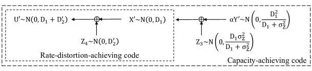
Figure 5: A test channel for the Gaussian Heegard-Berger problem for Decoder 2 using a continuous Gaussian $U^{\prime}$.

The final reconstruction at Decoder 2 is given by $\hat{X}_{2}=U_{1}+\alpha Y^{\prime}+\frac{1}{\gamma}\left(U^{\prime}-\alpha Y^{\prime}\right).$ Note that $\frac{1}{\gamma}\left(U^{\prime}-\alpha Y^{\prime}\right)$ is a scaled version of $Z_{5}$, which is independent of $Y^{\prime}$. Thus, the variance of $\alpha Y^{\prime}+\frac{1}{\gamma}\left(U^{\prime}-\alpha Y^{\prime}\right)$ is $\alpha D_{1}+\frac{1}{\gamma^{2}}\left(\gamma D_{2}+\alpha\sigma_{Z}^{2}\right)=D_{1}-D_{2}$. Therefore, we have $X-U_{1}=\hat{X}_{2}-U_{1}+\mathcal{N}\left(0,D_{2}\right)$ as we desired. Furthermore, the required data rate for Decoder 2 is then given by $R_{2}>I\left(U^{\prime};X^{\prime}\right)-I\left(U^{\prime};\alpha Y^{\prime}\right)=\frac{1}{2}\log\left(\frac{D_{1}\sigma_{Z}^{2}}{D_{2}\left(D_{1}+\sigma_{Z}^{2}\right)}\right).$

Note that $U^{\prime}$ is a continuous Gaussian random variable which is impractical for the design of polar lattices. Hence, we use the discrete Gaussian distribution $D_{\Lambda,\sigma_{U^{\prime}}^{2}}$ to replace it. Before that, we need to perform MMSE rescaling on $U^{\prime}$ for test channels $X^{\prime}\rightarrow U^{\prime}$ and $Y^{\prime}\rightarrow U^{\prime}$ with scales $\alpha_{q}$ and $\alpha_{c}$, respectively. Consequently, a reversed version of the test channel in Fig. 5 can be derived, as depicted in Fig. 6, where

$$\alpha_{q}=\frac{D_{1}}{D_{1}+D^{\prime}_{2}}=\frac{D_{1}\left(\sigma_{Z}^{2}-D_{2}\right)-D_{2}\sigma_{Z}^{2}}{D_{1}\left(\sigma_{Z}^{2}-D_{2}\right)}$$

and

$$\alpha_{c}=\frac{D_{1}^{2}}{\left(D_{1}+D^{\prime}_{2}\right)\left(D_{1}+\sigma_{Z}^{2}\right)}=\frac{D_{1}\left(\sigma_{Z}^{2}-D_{2}\right)-D_{2}\sigma_{Z}^{2}}{\left(D_{1}+\sigma_{Z}^{2}\right)\left(\sigma_{Z}^{2}-D_{2}\right)}.$$

The reconstruction of $X$ at Decoder 2 is as given in the following proposition.

Proposition 11.

If we use the reversed test channel shown in Fig 6, the reconstruction of $X$ at Decoder 2 is given by

$$\hat{X}_{2}=U_{1}+\alpha_{q}U^{\prime}+\eta\left(\frac{\alpha_{q}}{\alpha_{c}}\alpha Y^{\prime}-\alpha_{q}U^{\prime}\right),\textrm{ }\eta=\frac{D_{2}}{\sigma_{Z}^{2}}.$$

Proof:

It suffices to prove that $X-U_{1}=\hat{X}_{2}-U_{1}+\mathcal{N}\left(0,D_{2}\right)$. Since we have $X^{\prime}=\alpha_{q}U^{\prime}+\mathcal{N}\left(0,\alpha_{q}D^{\prime}_{2}\right)$, as illustrated in Fig 6, showing $\hat{X}_{2}-U_{1}=\alpha_{q}U^{\prime}+\mathcal{N}\left(0,\alpha_{q}D^{\prime}_{2}-D_{2}\right)$ would complete the proof. We can see from Fig 6 that $\frac{\alpha_{q}}{\alpha_{c}}\alpha Y^{\prime}-\alpha_{q}U^{\prime}$ is Gaussian distributed with zero mean and variance $\alpha_{q}D^{\prime}_{2}+\frac{\alpha_{q}}{\alpha_{c}}\sigma_{Z_{3}}^{2}$, and it is independent of $U^{\prime}$. We also have

$$\alpha_{q}D^{\prime}_{2}-D_{2} =\frac{D_{1}\left(\sigma_{Z}^{2}-D_{2}\right)-D_{2}\sigma_{Z}^{2}}{D_{1}\left(\sigma_{Z}^{2}-D_{2}\right)}\frac{D_{1}D_{2}\sigma_{Z}^{2}}{D_{1}\sigma_{Z}^{2}-D_{2}\left(D_{1}+\sigma_{Z}^{2}\right)}-D_{2}$$

$$=\frac{D_{2}^{2}}{\sigma_{Z}^{2}-D_{2}},$$

and

$$\eta^{2}\left(\alpha_{q}D^{\prime}_{2}+\frac{\alpha_{q}}{\alpha_{c}}\sigma_{Z_{3}}^{2}\right) =\left(\frac{D_{2}}{\sigma_{Z}^{2}}\right)^{2}\left(\frac{D_{2}\sigma_{Z}^{2}}{\left(\sigma_{Z}^{2}-D_{2}\right)}+\frac{D_{1}+\sigma_{Z}^{2}}{D_{1}}\frac{D_{1}\sigma_{Z}^{2}}{D_{1}+\sigma_{Z}^{2}}\right)$$

$$=\frac{D_{2}^{2}}{\sigma_{Z}^{2}-D_{2}},$$

as we desired. ∎

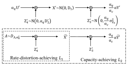
Figure 6: A reversed solution of the test channels in order to construct polar lattices.

Based on the reversed test channel, we can replace the continuous Gaussian random variable $\alpha_{q}U^{\prime}$ with a discrete Gaussian distributed variable $A\sim D_{\varLambda,\sigma_{a}^{2}}$, where $\sigma_{a}^{2}=\alpha_{q}^{2}\sigma_{U^{\prime}}^{2}$. Let $\bar{X^{\prime}}\triangleq A+\mathcal{N}\left(0,\alpha_{q}D^{\prime}_{2}\right)$ and $\frac{\alpha_{q}}{\alpha_{c}}\alpha\bar{Y^{\prime}}=\bar{X^{\prime}}+\mathcal{N}\left(0,\frac{\alpha_{q}}{\alpha_{c}}\sigma_{Z_{3}}^{2}\right)$. We also define $\bar{B}\triangleq\frac{\alpha_{q}}{\alpha_{c}}\alpha\bar{Y^{\prime}}$, whose variance is $\sigma_{b}^{2}=\frac{\alpha_{q}^{2}}{\alpha_{c}^{2}}\alpha^{2}\sigma_{Y^{\prime}}^{2}$. By [6, Lemma 1], the distributions of $\bar{X^{\prime}}$ and $\bar{Y^{\prime}}$ can be made arbitrarily close to the distributions of $X^{\prime}$ and $Y^{\prime}$, respectively. Therefore, polar lattices can be designed for the source $\bar{X^{\prime}}$ and the side information $\bar{Y^{\prime}}$ at Decoder 2. Specifically, a rate-distortion bound-achieving polar lattice $L_{1}$ is constructed for the source $\bar{X^{\prime}}$ with distortion $\alpha_{q}D^{\prime}_{2}$, and an AWGN capacity-achieving polar lattice $L_{2}$ is constructed for the channel $A\rightarrow\frac{\alpha_{q}}{\alpha_{c}}\alpha\bar{Y^{\prime}}$, as shown in Fig. 6. In the end, the reconstruction of Decoder 2 is $\check{X_{2}}=U_{1}+A+\eta\left(\bar{B}-A\right)$. Even though the quantization noise of $L_{1}$ is not an exact Gaussian distribution, it is shown in [6, Theorem 4] that the two distributions can be arbitrarily close when $N$ is sufficiently large. Therefore, $\bar{B}-A$ can be treated as Gaussian noise independent of $A$. By Proposition 11, $\eta$ scales $\bar{B}-A$ to $\mathcal{N}\left(0,\alpha_{q}D^{\prime}_{2}-D_{2}\right)$ and by [6, Lemma 1], the distributions of $\check{X_{2}}$ and $\hat{X}_{2}$ can be arbitrarily close, which gives an average distortion close to $D_{2}$.

According to [11, Lemma 10], $L_{1}$ and $L_{2}$ can be equivalently constructed for the MMSE-rescaled channel with Gaussian noise variances

$$\tilde{\sigma_{q}^{2}}=\frac{\sigma_{a}^{2}}{D_{1}}\alpha_{q}D^{\prime}_{2}=\frac{\sigma_{a}^{2}\sigma_{Z}^{2}D_{2}}{D_{1}\left(\sigma_{Z}^{2}-D_{2}\right)},$$

and

$$\tilde{\sigma_{c}^{2}}=\frac{\sigma_{a}^{2}}{\sigma_{b}^{2}}\left(\alpha_{q}D^{\prime}_{2}+\frac{\alpha_{q}}{\alpha_{c}}\sigma_{Z_{3}}^{2}\right)=\frac{\sigma_{a}^{2}\sigma_{Z}^{4}}{\left(D_{1}+\sigma_{Z}^{2}\right)\left(\sigma_{Z}^{2}-D_{2}\right)}.$$

The coding strategy for $L_{1}$ and $L_{2}$ can be adapted from [6, Section V]. We briefly describe it for completeness. First, choose a good constellation $D_{\varLambda,\sigma_{a}^{2}}$ such that the flatness factor $\epsilon_{\Lambda}(\tilde{\sigma_{q}^{2}})$ is negligible. Let $\Lambda/\Lambda_{1}/\cdots/\Lambda_{r-1}/\Lambda_{r}/\cdots$ denote a one-dimensional binary partition chain labeled by bits $A_{1}/A_{2}/\cdots/A_{r-1}/A_{r}/\cdots$. Therefore, $P_{A_{1:r}}$ and $A_{1:r}$ approaches $D_{\varLambda,\sigma_{a}^{2}}$ and $A$, respectively, as $r\rightarrow\infty$. Consider $N$ i.i.d copies of $A$, and let $K_{l}^{1:N}\triangleq A_{l}^{1:N}G_{N}$ for each level $1\leq l\leq r$. For $0<\beta<0.5$, the frozen set $\mathcal{F}_{l}^{Q}\left(\mathcal{F}_{l}^{C}\right)$, information set $\mathcal{I}_{l}^{Q}\left(\mathcal{I}_{l}^{C}\right)$, and shaping set $\mathcal{S}_{l}^{Q}\left(\mathcal{S}_{l}^{C}\right)$ for $L_{1}\left(L_{2}\right)$ at level $l$ can be adapted from [6, Equation (35)] and [6, Equation (36)], respectively, by replacing $\bar{X}$ with $\bar{X^{\prime}}$.

Furthermore, according to [6, Lemma 2], $L_{2}$ is nested within $L_{1}$, i.e., $L_{2}\subseteq L_{1}$. By the fact $\tilde{\sigma_{q}^{2}}\leq\tilde{\sigma_{c}^{2}}$ and [11, Lemma 3], the partition channel $\Lambda_{l-1}/\Lambda_{l}$ with noise variance $\tilde{\sigma_{c}^{2}}$ is degraded with respect to the one with noise variance $\tilde{\sigma_{q}^{2}}$. Therefore, we have $\mathcal{F}_{l}^{Q}\subseteq\mathcal{F}_{l}^{C}$, $\mathcal{I}_{l}^{C}\subseteq\mathcal{I}_{l}^{Q}$, and by the definition of shaping set, we observe that $\mathcal{S}_{l}^{Q}\subseteq\mathcal{S}_{l}^{C}$.

The encoder can recover the auxiliary codeword $U_{1}^{1:N}$ for Decoder 1, and obtains the realizations $x^{\prime 1:N}$ $\left(y^{\prime 1:N}\right)$ of $X^{\prime 1:N}=X^{1:N}-U_{1}^{1:N}\left(Y^{\prime 1:N}=Y^{1:N}-U_{1}^{1:N}\right)$ from given realizations of variables $X^{1:N}\left(Y^{1:N}\right)$, respectively. The encoder recovers $k_{l}^{1:N}$ from $l=[r]$ successively according to the random rounding quantization rules given in [6, Equations (13), (14), (17) and (18)]. Note that $x^{\prime 1:N}$ as realization of $\bar{X^{\prime}}{}^{1:N}$ is acceptable since the distributions of $X^{\prime}$ and $\bar{X^{\prime}}$ are arbitrarily close. Also, according to [6, Theorem 2], replacing the random rounding rule with MAP decision to obtain $k_{l}^{\mathcal{S}_{l}^{Q}}$ will not affect [11, Theorem 5] and [11, Theorem 6]. Consequently, the coding scheme for Decoder 2 for the Gaussian Heegard-Berger problem can be summarized as following:

Encoding: From the $N$-dimensional i.i.d. source vector $X^{1:N}$, the encoder recovers the auxiliary codeword $U_{1}^{1:N}$ employing a quantization polar lattice for source $X$ with variance $\sigma_{X}^{2}$ and distortion $D_{1}$, and obtains $X^{\prime 1:N}$ and $Y^{\prime 1:N}$. Next, the encoder evaluates $K_{l}^{\mathcal{I}_{l}^{Q}}$ by random rounding and sends $K_{l}^{\mathcal{I}_{l}^{Q}\backslash\mathcal{I}_{l}^{C}}$ to the decoders.

Decoding: By the pre-shared $K_{l}^{\mathcal{F}_{l}^{Q}}$ and received $K_{l}^{\mathcal{I}_{l}^{Q}\backslash\mathcal{I}_{l}^{C}}$, Decoder 2 recovers $K_{l}^{\mathcal{I}_{l}^{C}}$ and $K_{l}^{\mathcal{S}_{l}^{Q}}$ from the side information $\bar{B}^{1:N}$ with vanishing error probability, by using SC decoding for Gaussian channels [11]. At each level, Decoder 2 obtains $K_{l}^{1:N}$, and $A^{1:N}$ can be recovered according to [6, Equation (38)]. Finally, the reconstruction of Decoder 2 is

$$\check{X_{2}}^{1:N}=U_{1}^{1:N}+A^{1:N}+\eta\left(\bar{B}^{1:N}-A^{1:N}\right).$$ (9)

According to [11, Lemma 8], the encoding and decoding complexities of polar lattices remain to be $O\left(N\log N\right)$.

As for the transmission rate of this scheme, the rate $R_{1}$ for Decoder 1 can be arbitrarily close to $\frac{1}{2}\log\left(\frac{\sigma_{X}^{2}}{D_{1}}\right)$ according to [6, Theorem 4]. By the same argument, the rate $R_{L_{1}}$ of $L_{1}$ can be arbitrarily close to $\frac{1}{2}\log\left(\frac{D_{1}}{\alpha_{q}D^{\prime}_{2}}\right)$ when the flatness factor is negligible. By [11, Theorem 7], the rate $R_{L_{2}}$ of the capacity-achieving lattice $L_{2}$ can be arbitrarily close to $\frac{1}{2}\log\left(\frac{\sigma_{b}^{2}}{\alpha_{q}D^{\prime}_{2}+\frac{\alpha_{q}}{\alpha_{c}}\sigma_{Z_{3}}^{2}}\right)$ with a negligible flatness factor. Since $L_{2}\subseteq L_{1}$, the rate for Decoder 2 after some tedious calculations is given by

$$R_{2}=R_{L_{1}}-R_{L_{2}} \rightarrow\frac{1}{2}\log\left(\frac{D_{1}\left(\sigma_{Z}^{2}-D_{2}\right)}{D_{2}\sigma_{Z}^{2}}\right)-\frac{1}{2}\log\left(\frac{\left(D_{1}+\sigma_{Z}^{2}\right)\left(\sigma_{Z}^{2}-D_{2}\right)}{\sigma_{Z}^{4}}\right)$$

$$\rightarrow\frac{1}{2}\log\left(\frac{D_{1}\sigma_{Z}^{2}}{D_{2}\left(D_{1}+\sigma_{Z}^{2}\right)}\right),$$

and the total rate for the Gaussian Heegard-Berger problem is

$$R_{1}+R_{2}\rightarrow\frac{1}{2}\log\left(\frac{\sigma_{X}^{2}\sigma_{Z}^{2}}{D_{2}\left(D_{1}+\sigma_{Z}^{2}\right)}\right),$$

which is the same as (2).

Next, we give the main theorem of the Gaussian Heegard-Berger problem for the non-degenerate region.

Theorem 12.

Let $\left(X,Y,Z,D_{1},D_{2}\right)$ be as specified in Section II-C. For any rate $R_{1}>\frac{1}{2}\log\left(\frac{\sigma_{X}^{2}}{D_{1}}\right)$, there exists a polar lattice code at rate $R_{1}$ with sufficiently large blocklength, whose expected distortion is arbitrarily close to $D_{1}$ and the number of partition levels is $O\left(\log\log N\right)$. Let $\Lambda/\Lambda_{1}/\cdots/\Lambda_{r-1}/\Lambda_{r}$ be a one-dimensional binary partition chain of a lattice $\Lambda$ such that $\epsilon_{\Lambda}(\tilde{\sigma_{q}^{2}})=O\left(2^{-\sqrt{N}}\right)$ and $r=O\left(\log N\right)$. For any $0<\beta^{\prime}<\beta<0.5$, there exist nested polar lattices $L_{1}$ and $L_{2}$ with a rate spread $R_{2}=R_{L_{1}}-R_{L_{2}}$ arbitrarily close to $\frac{1}{2}\log\left(\frac{D_{1}\sigma_{Z}^{2}}{D_{2}\left(D_{1}+\sigma_{Z}^{2}\right)}\right)$ such that the expected distortion $D_{Q_{2}}$ satisfies $D_{Q_{2}}\leq D_{2}+O\left(2^{-N^{\beta^{\prime}}}\right)$.

Proof:

The achievability of the rate-distortion function for Decoder 1 follows from [6, Theorem 4]. The proof of the achievability for Decoder 2 can be adapted from [6, Theorem 5], by considering the test channel depicted in Fig. 6 and the reconstruction as given by (9). It is worth mentioning that the requirements $\epsilon_{\Lambda}(\tilde{\sigma_{q}^{2}})=O\left(2^{-\sqrt{N}}\right)$ and $r=O\left(\log N\right)$ are given by [6, Proposition 2] to guarantee a sub-exponentially decaying error probability for the lattice design for Decoder 2. ∎

V Conclusion

We presented nested polar codes and polar lattices that achieve the rate-distortion function for the binary and Gaussian Heegard-Berger problems, respectively. Different from the code constructions for the Wyner-Ziv problem [5] and [6], we took advantage of the reconstruction at Decoder 1 to build the nested structure that achieves the rate-distortion function for Decoder 2. The proposed schemes achieve the HBRDF in the entire non-degenerate regions for both DSBS and Gaussian sources.

Finally, the Kaspi problem in [14] is regarded as a generalization of the Heegard-Berger problem, where the encoder may also have access to the side information. The explicit rate-distortion functions for the Kaspi problem with Gaussian and binary sources have been given in [15] and [16], respectively. We will study the construction of polar codes and polar lattices for the Kaspi problem in our future work.

Appendix A Proof of Theorem 9

First, we show that the distortion $D_{2}$ can be achieved. Since $U_{b}^{1:N}=W^{1:N}G_{N}$ gives a one-to-one mapping between $W^{1:N}$ and $U_{b}^{1:N}$, expression (8) is equivalent to

$$\mathbb{V}\left(P_{U_{a}^{1:N},U_{b}^{1:N},X^{1:N},U_{1}^{1:N}},Q_{U_{a}^{1:N},U_{b}^{1:N},X^{1:N},U_{1}^{1:N}}\right)=O\left(2^{-N^{\beta^{\prime}}}\right).$$ (10)

From the coding scheme presented in Section III-B, we assume that $K_{\mathcal{I}_{C_{a}}}$ and $W_{\mathcal{I}_{C_{b}}}$can be correctly decoded by using side information, and $K_{\mathcal{S}_{S_{a}}}$ and $W_{\mathcal{S}_{S_{b}}}$ can be recovered by the MAP rule. Therefore, Decoder 2 can recover $U_{a}^{1:N}$ and $U_{b}^{1:N}$ with the joint distribution $Q_{U_{a}^{1:N},U_{b}^{1:N},X^{1:N},U_{1}^{1:N}}$. Denote by $Q_{U_{a}^{1:N},U_{b}^{1:N},X^{1:N},U_{1}^{1:N},Y^{1:N}}$ the resulting distribution when the encoder performs compression at each level, i.e., compresses $X^{1:N}$ to $W_{\mathcal{I}_{S_{b}}}$. Let $P_{U_{a}^{1:N},U_{b}^{1:N},X^{1:N},U_{1}^{1:N},Y^{1:N}}$ denote the joint distribution when the encoder does not perform compression. For simplicity, we denote random variables $U_{1}^{1:N}$, $U_{a}^{1:N}$ and $U_{b}^{1:N}$ by $U_{1,a,b}^{1:N}$.

$$2\mathbb{V}\left(P_{U_{1,a,b}^{1:N},X^{1:N},Y^{1:N}},Q_{U_{1,a,b}^{1:N},X^{1:N},Y^{1:N}}\right)$$

$$=\sum_{u_{1,a,b}^{1:N},x^{1:N},y^{1:N}}\left|P\left(u_{1,a,b}^{1:N},x^{1:N},y^{1:N}\right)-Q\left(u_{1,a,b}^{1:N},x^{1:N},y^{1:N}\right)\right|$$

$$=\sum_{u_{1,a,b}^{1:N},x^{1:N},y^{1:N}}\left|P\left(u_{1,a,b}^{1:N},x^{1:N}\right)P\left(y^{1:N}|u_{1,a,b}^{1:N},x^{1:N}\right)-Q\left(u_{1,a,b}^{1:N},x^{1:N}\right)Q\left(y^{1:N}|u_{1,a,b}^{1:N},x^{1:N}\right)\right|.$$

According to the Markov chain $Y\leftrightarrow X\leftrightarrow U_{1,a,b}^{1:N}$, we have

$$P\left(y^{1:N}|u_{1,a,b}^{1:N},x^{1:N}\right)=Q\left(y^{1:N}|u_{1,a,b}^{1:N},x^{1:N}\right)=P\left(y^{1:N}|x^{1:N}\right).$$

Therefore,

$$\mathbb{V}\left(P_{U_{1,a,b}^{1:N},X^{1:N},Y^{1:N}},Q_{U_{1,a,b}^{1:N},X^{1:N},Y^{1:N}}\right)=\mathbb{V}\left(P_{U_{1,a,b}^{1:N},X^{1:N}},Q_{U_{1,a,b}^{1:N},X^{1:N}}\right)=O\left(2^{-N^{\beta^{\prime}}}\right).$$ (11)

The reconstructions of two levels are $U_{a}^{1:N}$ and $U_{b}^{1:N}$ (i.e., denoted by $U_{a,b}^{1:N}$), and the average distortion $D_{P}$ achieved by $P_{U_{1,a,b}^{1:N},X^{1:N},Y^{1:N}}$ is given by

$$D_{P} =\frac{1}{N}\sum_{u_{1,a,b}^{1:N},x^{1:N},y^{1:N}}P_{U_{1,a,b}^{1:N},X^{1:N},Y^{1:N}}\left(u_{1,a,b}^{1:N},x^{1:N},y^{1:N}\right)d\left(U_{a,b}^{1:N},x^{1:N}\right)$$

$$=\frac{1}{N}\sum_{u_{a,b}^{1:N},x^{1:N}}P_{U_{a,b}^{1:N},X^{1:N}}\left(u_{a,b}^{1:N},x^{1:N}\right)d\left(U_{a,b}^{1:N},x^{1:N}\right)$$

$$=\frac{1}{N}N\sum_{u_{a,b},x}P_{U_{a,b},X}\left(u_{a,b},x\right)d\left(U_{a,b},x\right)$$

$$=D_{2}.$$

Note that the last equality holds due to the constrains $\left(\theta-\theta_{1}\right)\alpha+\theta_{1}\mu+\left(1-\theta\right)p=D_{2}$ of Theorem 4. This is reasonable because $D_{P}$ is achieved when the encoder does not perform any compression. Combined with (11), the expected distortion $D_{Q}$ achieved by $Q_{U_{1,a,b}^{1:N},X^{1:N},Y^{1:N}}$ satisfies

$$D_{Q}-D_{P} =\frac{1}{N}\sum_{u_{1,a,b}^{1:N},x^{1:N},y^{1:N}}\left(Q_{U_{1,a,b}^{1:N},X^{1:N},Y^{1:N}}-P_{U_{1,a,b}^{1:N},X^{1:N},Y^{1:N}}\right)d\left(U_{a,b}^{1:N},x^{1:N}\right)$$

$$\leq\frac{1}{N}Nd_{\max}\sum_{u_{1,a,b}^{1:N},x^{1:N},y^{1:N}}\left|P_{U_{1,a,b}^{1:N},X^{1:N},Y^{1:N}}-Q_{U_{1,a,b}^{1:N},X^{1:N},Y^{1:N}}\right|$$

$$=O\left(2^{-N^{\beta^{\prime}}}\right).$$

Next we show that the decoder can recover $U_{a}^{i\in\mathcal{I}_{C_{a}}}$ and $U_{b}^{i\in\mathcal{I}_{C_{b}}}$ with a sub-exponentially decaying block error probability.

$$2\mathbb{V}\left(P_{U_{1,a,b}^{1:N},Y^{1:N}},Q_{U_{1,a,b}^{1:N},Y^{1:N}}\right) =\sum_{u_{1,a,b}^{1:N},y^{1:N}}\left|P\left(u_{1,a,b}^{1:N},y^{1:N}\right)-Q\left(u_{1,a,b}^{1:N},y^{1:N}\right)\right|$$

$$=\sum_{u_{1,a,b}^{1:N},y^{1:N}}\left|\sum_{x^{1:N}}\left[P\left(u_{1,a,b}^{1:N},x^{1:N},y^{1:N}\right)-Q\left(u_{1,a,b}^{1:N},x^{1:N},y^{1:N}\right)\right]\right|$$

$$\leq\sum_{u_{1,a,b}^{1:N},y^{1:N}}\sum_{x^{1:N}}\left|P\left(u_{1,a,b}^{1:N},x^{1:N},y^{1:N}\right)-Q\left(u_{1,a,b}^{1:N},x^{1:N},y^{1:N}\right)\right|$$

$$=O\left(2^{-N^{\beta^{\prime}}}\right).$$

Let $E_{P}^{a}\left[Pe\right]$ and $E_{P}^{b}\left[Pe\right]$ denote the expectation error probability as a result of the distribution $P_{U_{1,a,b}^{1:N},Y^{1:N}}$ at level 1 and 2, respectively. Take $E_{P}^{b}\left[Pe\right]$ as an example to show the decaying error probability. Let $\mathcal{E}_{i}$ denote the set of random variables $\left(u_{b}^{1:N},u_{1,a}^{1:N},y^{1:N}\right)$ such that the SC decoding error occurred at the $i$th bit. Hence the block error event is defined by $\mathcal{E}^{b}\triangleq\cup_{i\in\mathcal{I}_{C_{b}}}\mathcal{E}_{i}$, and the expectation of decoding block error probability over all random mapping is given by

$$E_{P}^{b}\left[Pe\right] =\sum_{u_{1,a,b}^{1:N},y^{1:N}}P_{U_{1,a,b}^{1:N},Y^{1:N}}\left(u_{1,a,b}^{1:N},y^{1:N}\right)\boldsymbol{1}\left[\left(u_{b}^{1:N},u_{1,a}^{1:N},y^{1:N}\right)\in\mathcal{E}^{b}\right]$$

$$\leq\sum_{i\in\mathcal{I}_{C_{b}}\cup\mathcal{S}_{S_{b}}}\sum_{u_{1,a,b}^{1:N},y^{1:N}}P_{U_{1,a,b}^{1:N},Y^{1:N}}\left(u_{1,a,b}^{1:N},y^{1:N}\right)\boldsymbol{1}\left[\left(u_{b}^{1:N},u_{1,a}^{1:N},y^{1:N}\right)\in\mathcal{E}_{i}\right]$$

$$\leq\sum_{i\in\mathcal{I}_{C_{b}}\cup\mathcal{S}_{S_{b}}}\sum_{u_{b}^{1:i},u_{1,a}^{1:N},y^{1:N}}P\left(u_{b}^{1:i-1},u_{1,a}^{1:N},y^{1:N}\right)P\left(u_{b}^{i}|u_{b}^{1:i-1},u_{1,a}^{1:N},y^{1:N}\right)$$

$$\hskip 85.35826pt\cdot\boldsymbol{1}\left[P\left(u_{b}^{i}|u_{b}^{1:i-1},u_{1,a}^{1:N},y^{1:N}\right)\leq P\left(u_{b}^{i}\oplus 1|u_{b}^{1:i-1},u_{1,a}^{1:N},y^{1:N}\right)\right]$$

$$\leq\sum_{i\in\mathcal{I}_{C_{b}}\cup\mathcal{S}_{S_{b}}}\sum_{u_{b}^{1:i},u_{1,a}^{1:N},y^{1:N}}P\left(u_{b}^{1:i-1},u_{1,a}^{1:N},y^{1:N}\right)P\left(u_{b}^{i}|u_{b}^{1:i-1},u_{1,a}^{1:N},y^{1:N}\right)$$

$$\hskip 85.35826pt\cdot\sqrt{\frac{P\left(u_{b}^{i}\oplus 1|u_{b}^{1:i-1},u_{1,a}^{1:N},y^{1:N}\right)}{P\left(u_{b}^{i}|u_{b}^{1:i-1},u_{1,a}^{1:N},y^{1:N}\right)}}$$

$$\leq N\cdot Z\left(U_{b}^{i}|U_{b}^{1:i-1},U_{1,a}^{1:N},Y^{1:N}\right)$$

$$=O\left(2^{-N^{\beta^{\prime}}}\right).$$

Following the same arguments, we also have $E_{P}^{a}\left[Pe\right]=O\left(2^{-N^{\beta^{\prime}}}\right)$. Therefore, by this union bound, we obtain the two-stage decoding block error probability $E_{P}\left[Pe\right]=O\left(2^{-N^{\beta^{\prime}}}\right)$.

Let $Pe^{HB}$ denote the expectation of error probability caused by $Q_{U_{1,a,b}^{1:N},Y^{1:N}}$, which is an average over all choices of $U_{a}^{i\in\mathcal{F}_{C_{a}}}$, $U_{a}^{i\in\mathcal{S}_{C_{a}}\backslash\mathcal{S}_{S_{a}}}$, $U_{b}^{i\in\mathcal{F}_{C_{b}}}$ and $U_{b}^{i\in\mathcal{S}_{C_{b}}\backslash\mathcal{S}_{S_{b}}}$at each level. Let $\mathcal{E}$ denote the set of random variables $\left(u_{b}^{1:N},u_{1,a}^{1:N},y^{1:N}\right)$ such that a decoding error occurs. Then we have

$$Pe^{HB}-E_{P}\left[Pe\right] =\sum_{u_{1,a,b}^{1:N},y^{1:N}}\left(Q\left(u_{1,a,b}^{1:N},y^{1:N}\right)-P\left(u_{1,a,b}^{1:N},y^{1:N}\right)\right)\cdot\boldsymbol{1}\left[\left(u_{b}^{1:N},u_{1,a}^{1:N},y^{1:N}\right)\in\mathcal{E}\right]$$

$$\leq 2\mathbb{V}\left(P_{U_{1,a,b}^{1:N},Y^{1:N}},Q_{U_{1,a,b}^{1:N},Y^{1:N}}\right)$$

$$\leq O\left(2^{-N^{\beta^{\prime}}}\right).$$

As for the rates, we have $\frac{\left|\mathcal{I}_{S_{a}}\right|}{N}\xrightarrow{N\rightarrow\infty}I\left(U_{a};X,U_{1}\right)$ and $\frac{\left|\mathcal{I}_{C_{a}}\right|}{N}\xrightarrow{N\rightarrow\infty}I\left(U_{a};Y,U_{1}\right)$ at the first level. Therefore, we have

$$\frac{\left|\mathcal{I}_{S_{a}}\right|-\left|\mathcal{I}_{C_{a}}\right|}{N}\xrightarrow{N\rightarrow\infty}I\left(X;U_{a}|U_{1},Y\right).$$

For the second level, $\frac{\left|\mathcal{I}_{S_{b}}\right|}{N}\xrightarrow{N\rightarrow\infty}I\left(U_{b};X,U_{1},U_{a}\right)$ and $\frac{\left|\mathcal{I}_{C_{b}}\right|}{N}\xrightarrow{N\rightarrow\infty}I\left(U_{b};Y,U_{1},U_{a}\right)$. Thus, we have

$$\frac{\left|\mathcal{I}_{S_{b}}\right|-\left|\mathcal{I}_{C_{b}}\right|}{N}\xrightarrow{N\rightarrow\infty}I\left(X;U_{b}|U_{1},U_{a},Y\right).$$

Finally, the rate of Decoder 2 is

$$\frac{\left|\mathcal{I}_{S_{a}}\right|-\left|\mathcal{I}_{C_{a}}\right|+\left|\mathcal{I}_{S_{b}}\right|-\left|\mathcal{I}_{C_{b}}\right|}{N}\xrightarrow{N\rightarrow\infty}I\left(X;U_{2}|U_{1},Y\right).$$

References

- [1] A. Wyner and J. Ziv, “The rate-distortion function for source coding with side information at the decoder,” IEEE Trans. Inf. Theory, vol. 22, no. 1, pp. 1–10, Jan 1976.
- [2] C. Heegard and T. Berger, “Rate distortion when side information may be absent,” IEEE Trans. Inf. Theory, vol. 31, no. 6, pp. 727–734, 1985.
- [3] K. Kerpez, “The rate-distortion function of a binary symmetric source when side information may be absent,” IEEE Trans. Inf. Theory, vol. 33, no. 3, pp. 448–452, May 1987.
- [4] C. Tian and S. N. Diggavi, “A calculation of the Heegard-Berger rate-distortion function for a binary source,” in Proc. 2006 IEEE Inform. Theory Workshop, Oct 2006, pp. 342–346.
- [5] S. B. Korada, “Polar codes for channel and source coding,” Ph.D. dissertation, Ecole Polytechnique Fédérale de Lausanne, Lausanne, Switzerland, 2009.
- [6] L. Liu and C. Ling, “Polar lattices for lossy compression,” Jan. 2015. [Online]. Available: http://arxiv.org/abs/1501.05683
- [7] J. Honda and H. Yamamoto, “Polar coding without alphabet extension for asymmetric models,” IEEE Trans. Inf. Theory, vol. 59, no. 12, pp. 7829–7838, Dec. 2013.
- [8] M. Ye and A. Barg, “Polar codes for distributed hierarchical source coding,” Advances in Mathematics of Communications, vol. 9, no. 1, pp. 87–103, 2015.
- [9] S. Ramanan and J. M. Walsh, “Practical codes for lossy compression when side information may be absent,” Proc. IEEE Int. Conf. on Acoustics, Speech and Signal Processing, pp. 3048–3051, May 2011.
- [10] S. Korada and R. Urbanke, “Polar codes are optimal for lossy source coding,” IEEE Trans. Inf. Theory, vol. 56, no. 4, pp. 1751–1768, 2010.
- [11] Y. Yan, L. Liu, C. Ling, and X. Wu, “Construction of capacity-achieving lattice codes: Polar lattices,” Nov. 2014. [Online]. Available: http://arxiv.org/abs/1411.0187
- [12] G. D. Forney Jr., M. Trott, and S.-Y. Chung, “Sphere-bound-achieving coset codes and multilevel coset codes,” IEEE Trans. Inf. Theory, vol. 46, no. 3, pp. 820–850, May 2000.
- [13] C. Ling and J.-C. Belfiore, “Achieving AWGN channel capacity with lattice Gaussian coding,” IEEE Trans. Inf. Theory, vol. 60, no. 10, pp. 5918–5929, Oct. 2014.
- [14] A. H. Kaspi, “Rate-distortion function when side-information may be present at the decoder,” IEEE Trans. Inf. Theory, vol. 40, no. 6, pp. 2031–2034, 1994.
- [15] E. Perron, S. N. Diggavi, and I. E. Telatar, “The Kaspi rate-distortion problem with encoder side-information: Gaussian case,” Nov 2005. [Online]. Available: https://infoscience.epfl.ch/record/59938
- [16] ——, “The Kaspi rate-distortion problem with encoder side-information: Binary erasure case,” 2006. [Online]. Available: https://infoscience.epfl.ch/record/96000