Void profile from Planck lensing potential map

Abstract

We use the lensing potential map from Planck CMB lensing reconstruction analysis and the “Public Cosmic Void Catalog” to measure the stacked void lensing potential. In this profile, four parameters are needed to describe the shape of voids with different characteristic radii $R_{V}$. However, we have found that after reducing the background noise by subtracting the average background, there is a residue lensing power left in the data. The inclusion of the environment shifting parameter, $\gamma_{V}$, is necessary to get a better fit to the data with the residue lensing power. We divide the voids into two redshift bins: cmass1 ($0.45<z<0.5$) and cmass2 ($0.5<z<0.6$). Our best-fit parameters are $\alpha=1.989\pm 0.149$, $\beta=12.61\pm 0.56$, $\delta_{c}=-0.697\pm 0.025$, $R_{S}/R_{V}=1.039\pm 0.030$, $\gamma_{v}=(-7.034\pm 0.150)\times 10^{-2}$ for the cmass1 sample with 123 voids and $\alpha=1.956\pm 0.165$, $\beta=12.91\pm 0.60$, $\delta_{c}=-0.673\pm 0.027$, $R_{S}/R_{V}=1.115\pm 0.032$, $\gamma_{v}=(-4.512\pm 0.114)\times 10^{-2}$ for the cmass2 sample with 393 voids at 68% C.L. The addition of the environment parameter is consistent with the conjecture that the Sloan Digital Sky Survey voids reside in an underdense region.

1. Introduction

In the standard cosmological model, the universe is homogeneous and isotropic on large scales. The seeds of present-day large-scale structure of the universe are formed from the highly Gaussian and nearly scale-invariant power spectrum of matter density (Hinshaw et al., 2013; Planck Collaboration et al., 2016c). However, on small scales, the hierarchical clustering of matter leads to formations of complex cosmic structure such as clusters of galaxies, walls, filaments, and voids (Boylan-Kolchin et al., 2009). Among all of the large-scale objects in the universe, cosmic voids, which are large underdensities in the matter distribution, occupy the vast majority of the universe and hence provide the largest volume-based test on theories of structure formation (Ceccarelli et al., 2006). Being interesting objects in their own right, they contain a wealth of information on the fundamental properties of the universe. For example, the low-density environment of voids is a perfect place to study galaxies, as the galaxies are expected not to be affected by the complex astrophysical processes that modify galaxies in high-density environments and allows galaxies to evolve independently without environmental effects (Beygu et al., 2013; Penny et al., 2015). In addition, since voids occupy the cosmic volume where the matter density is lowest, the difference between dark energy and modified gravity models for cosmic acceleration could be distinguishable within cosmic voids (Clampitt et al., 2013; Cai et al., 2015; Barreira et al., 2015; Zivick et al., 2015).

The computational approach called $N$-body dark matter simulations is one of the best tools to empirically understand various void properties such as number functions (Sheth & van de Weygaert, 2004; Jennings et al., 2013) and void ellipticity functions (Biswas et al., 2010). However, the definition of voids is rather vague, and various definitions exist in the literature; some are more suitable for theoretical calculations, while the others are more suitable for observations or $N$-body simulations. This variety of definitions renders comparison of theoretical predictions on void properties and observations difficult. ZOBOV (Zones Bordering On Voidness; Neyrinck (2008)) and WVF (Watershed Void Finder;Platen et al. (2007)) are two of the popular void-finding algorithms. Both methods are based on some tessellation methods and the watershed concept of defining voids. ZOBOV requires no free parameters or assumptions about the shape and is based on Voronoi tessellation. However, the ZOBOV voids are unsmooth and rather edgy. WVF also requires no free parameters and is based on a watershed transform. However, WVF uses several techniques to smooth the density field so that the WVF voids are not edgy. With void identification algorithms being progressively developed for galaxy redshift surveys such as the Sloan Digital Sky Survey (SDSS), cosmic voids are being continually found, amounting to releases of public voids catalogs (Pan et al., 2012; Sutter et al., 2012b, 2014a; Nadathur, 2016).

Recently, there has be an increasing amount of attention on voids as objects for various aspects of cosmological studies. The dynamic of voids and redshift-space distortion (Kaiser, 1987) is one of the probes of the growth of large-scale structure. The amount of dark matter in the universe could be obtained from the peculiar velocity fields (Courtois et al., 2012). The relationship between their extent angular size and the distance along the line of sight, known as the Alcock–Paczyński test (Alcock & Paczynski, 1979), is predicted to be a promising probe of dark energy by using a stacking method to obtain a statistically averaged shape of voids in 2D or 3D spaces. By stacking a large number of voids, one would expect the difference in radial and transverse direction to be directly related to the product of angular distance and the Hubble parameter (Lavaux & Wandelt, 2012; Sutter et al., 2012a, 2014b). Another geometrical study, the evolution of the ellipticity of voids, could be used as a tool in practice to constrain the dark energy equation of state (Lee & Park, 2009; Bos et al., 2012). The Integrated Sachs–Wolfe (ISW) effect (Sachs & Wolfe, 1967) caused by the evolution of the gravitational potential within voids can also be detected (Granett et al., 2008; Cai et al., 2014; Chen & Kantowski, 2015; Hotchkiss et al., 2015; Ilić et al., 2013; Planck Collaboration et al., 2016e).

The measurement of weak gravitational lensing probes the matter distribution by means of the deflection of light from the background sources. The trajectories of photons from background sources are bent toward gravitating matter due to the distortion of spacetime caused by gravitational lensing (Einstein, 1936). The scenario is reversed when voids are acting as the sources of gravitational lenses instead of dark matter. The delensing effect of voids has been investigated and recently observed through the distortions of background galaxies by a stacking method that enhances the signal (Higuchi et al., 2013; Krause et al., 2013; Melchior et al., 2014; Clampitt & Jain, 2015; Gruen et al., 2016).

The cosmic microwave background (CMB) radiation, which is the signal from surface of the last scattering surface, exists as the ubiquitous background for gravitational lensing. The gravitational anti-lensing effect of voids has been recently investigated by (Bolejko et al., 2013), (Chen et al., 2015), (Das & Spergel, 2009). The CMB signals that are lensed by multiple voids are also a promising tool to obtain good constraints on cosmological parameters (Chantavat et al., 2016). Planck (Planck Collaboration et al., 2016d) has released lensing potential maps from the CMB that utilized quadratic estimators that exploit the statistical anisotropy induced by lensing (Okamoto & Hu, 2003). From a theoretical point of view, if the matter density distribution within a void, known as a void profile, is known, then the lensing potential could be computed and vice versa. The statistical average void density profile known as the universal void profile (here after, HSW; Hamaus et al. (2014a)) has been released and potentially could be exploited to predict the lensing effect of voids at various sizes and redshifts with only a few parameters (more in §3). Hence, from the lensing potential data from Planck, one could, in principle, derive the HSW parameters. This would be a good consistency check if the HSW void profile could be reverse-engineered from observables.

The goals of this article are (1) to extract the stacked lensing potential from Planck lensing data by cross-correlation with voids from SDSS data (Sutter et al., 2014b), (2) to compare and cross-examine the derived HSW void parameters from the Planck lensing potential map with other methods, and (3) to better understand the effect of gravitational lensing from voids in the Planck lensing data. We shall begin with a description of the void catalog from the SDSS galaxy redshift survey (Sutter et al., 2014b) and Planck lensing data (Planck Collaboration et al., 2016d) in §2. The extraction and cross-correlation methods are also discussed. In §3, we describe the HSW void profile parameterization, and a brief overview of the gravitational lensing effect with voids is also introduced. Our parameter estimation is described in §4, and the results are shown in §5. The discussions and conclusions are given in §6. Throughout this article, our fiducial cosmological parameters are $\Omega_{M}=0.315$, $\Omega_{\Lambda}=0.685$, $H_{0}=67.3\ \text{km s}^{-1}\text{Mpc}^{-1}$, $w=-1$, and $\Omega_{k}=0$, which is consistent with a flat $\Lambda$CDM cosmology from Planck 2013 + WMAP polarization maximum likelihood cosmological parameters (Planck Collaboration et al., 2014).

2. Data and Methodology

This study utilizes the lensing potential measured from the lensed CMB maps to extract the potential in the vicinity around cosmic voids. Here, we describe the datasets and method for measuring the stacked voids’ lensing potential, which will be used to constrain the void density profile, as discussed further in §3.

2.1. Planck Lensing Potential map

The descriptions of data products and an overview of the scientific results of the Planck full-mission data release are given by Planck Collaboration et al. (2016a). Apart from CMB temperature, polarization frequency maps, and foreground component maps, the science team also released the reconstructed lensing potential map of the CMB (Planck Collaboration et al., 2016d). They applied quadratic lensing estimators and procedures described by Okamoto & Hu (2003) to the foreground-cleaned CMB map. The foreground-cleaned map was constructed from all the frequency band maps using the SMICA procedure (Planck Collaboration et al., 2016b). The contaminated regions of the SMICA map were further removed with the Galaxy, point-source, and SMICA-specific temperature and polarization masks, which leave $\approx\!67\%$ of the sky for the minimum-variance lensing reconstruction analysis. Given the sensitivity and angular resolutions of the Planck mission, the analysis thus results in the most significant measurement of the CMB lensing potential map to date.

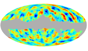
Figure 1.— Lensing potential map, $\psi(\hat{n})$, constructed from Planck lensing convergence, $\kappa_{\ell m}$. The gray shaded area marks the rejected pixels excluded by the analysis mask.

The online data provided by the Planck science team are in the standard HEALPix format (Górski et al., 2005). The spherical harmonics coefficients of lensing convergence, $\kappa_{\ell m}$, are given for multipoles up to $\ell_{\rm max}=2048$ instead of the lensing potential, $\psi_{\ell m}$. We use the standard definition of lensing convergence to calculate $\psi_{\ell m}$ from

$$\kappa_{\ell m}=\frac{\ell(\ell+1)}{2}\psi_{\ell m}.$$ (1)

We then use the HEALPix synfast package to synthesize the lensing potential map, $\psi(\hat{n})$. The generated map has a resolution of $N_{\rm side}=2048$ (i.e. $\approx 1^{\prime}.7\times 1^{\prime}.7$ pixels). The projected lensing potential map is shown in Figure. 1. This reconstructed lensing potential map is used to cross-correlate with the cosmic voids catalog, where the azimuthally averaged potential around each void is extracted, scaled, and then combined to constrain the void density profile. For our analysis, we shall use only those regions that pass the analysis mask (Galaxy + point-source + SMICA).

2.2. Cosmic voids catalogue

In this work, we use the “Public Cosmic Void Catalog” (Sutter et al., 2012b) constructed using a modified and extended version of the watershed algorithm ZOBOV, called ‘Void IDentification and Examination’ (VIDE; Sutter et al., 2014b). We applied the code to the SDSS Data Release 7 (Abazajian et al., 2009) main galaxy sample and SDSS-III Baryon Oscillation Spectroscopic Survey (BOSS) Data Release 10 (Ahn et al., 2014) LOWZ and CMASS samples. This results in $\approx 1\,500$ individually detected voids. The samples represent volume-limited catalogs of voids at various redshift bins.

To minimize any possible evolution of the profile parameters, we choose to work with voids in individual redshift bins and do not stack voids across the bins. In order to have as many voids in a single bin as possible, we chose a high-redshift bin to increase the volume. Here, we report on the analysis using the “dr10cmass1” ($0.45<z<0.5$, $\Delta t_{\rm age}=0.4{\rm\leavevmode\nobreak\ Gyrs}$, $N_{\rm void}=229$) and the “dr10cmass2” samples ($0.5<z<0.6$, $\Delta t_{\rm age}=0.7{\rm\leavevmode\nobreak\ Gyrs}$, $N_{\rm void}=696$), hereafter called “cmass1” and “cmass2,” respectively.

We therefore stacked the Planck lensing potential map (§2.1) around the central positions of cosmic voids taken from the Sutter et al. (2014b) “dr10cmass1” and “dr10cmass2” samples as two separated measurements. However, during our analysis we found that considerable numbers (106 and 303 for cmass1 and cmass2, respectively) of the voids are located in the negative lensing potential regions, which could be due to a number of reasons and warrants further investigations. We therefore restrict our analysis to 123 and 393 voids from samples cmass1 and cmass2, respectively. The radius and redshift distributions of the subsamples that we used do not show any significant difference from those of the excluded low-signal subsamples (see Figure. 2).

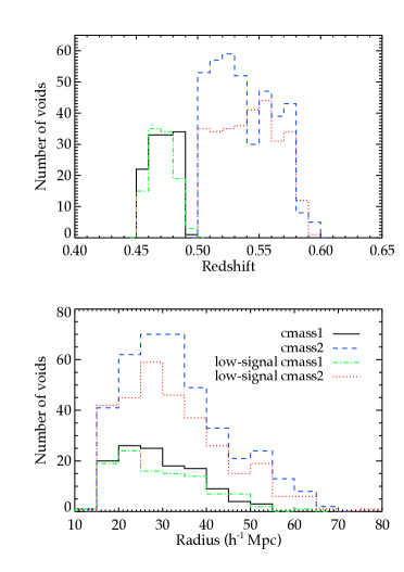
Figure 2.— Redshift (top) and radius (bottom) distributions of the void samples used in our analyses from the “dr10cmass1” (black solid lines) and “dr10cmass2” (blue dashed lines) samples, where their medians are $z_{\rm{cmass1}}=0.47$, $R_{V,\rm{cmass1}}=28.26\leavevmode\nobreak\ h^{-1}$Mpc and $z_{\rm{cmass2}}=0.53$, $R_{V,\rm{cmass2}}=31.68\leavevmode\nobreak\ h^{-1}$Mpc, respectively. For comparison, the redshift and radius distributions of voids rejected for the stacking analysis, as a result of a very weak lensing signal or having negative lensing potential, are also shown. We do not observe any significant deviation in their redshift and radius distributions.

2.3. Stacking analysis

The stacking analysis is performed on the Planck lensing potential map (See §2.1) around each of the voids’ centre. Since we need to compare our measurements to the theoretical prediction of the size-independent potential, $\tilde{\psi}(r/R_{V})$, (see Eq. (11) in §3.2), but the potential map is a 2D projection on the surface of a sphere, we therefore bin up the lensing potential according to physical separation and not angular separation. Therefore, for each void, we use the comoving angular diameter distance, $D_{A}(z)$, to scale the pixels of the lensing maps surrounding the vicinity of each void according to its redshift $z$ and radius $R_{V}$. For the $i$th $(r/R_{V})_{i}$ bin, its corresponding angular bin is given by

$$\theta_{i}\left(z,R_{V}\right)=R_{V}/D_{A}\left(z\right)\times(r/R_{V})_{i}.$$ (2)

The lensing potential value in each $r/R_{V}$ bin around a void is azimuthally averaged and is then background subtracted by the measurement at the largest separation, $10\,R_{V}$. Next, we scale the amplitude of the overall lensing potential measured from each void according to Eq. (LABEL:eq:scalefactor) to account for their different redshifts and radii before we combine them together. Each lensing potential is scaled to the its respective median redshift and radius,

$$\tilde{\psi}\left(r/R_{V}\right)_{i}=\psi\left(r;z,R_{V}\right)_{i}\times\frac{R_{V,\rm{med}}^{3}(1+z_{\rm med})^{3}D_{+}(z_{\rm med})D_{A}(z)}{R_{V}^{3}(1+z)^{3}D_{+}(z)D_{A}(z_{\rm med})},$$ (3)

where $R_{V,\rm{med}}$ and $z_{\rm med}$ are the median void radius and redshift, respectively, of the bins given in Figure. 2. The average lensing potential is then calculated from the scaled measurements of 123 and 393 voids for cmass1 and cmass2 samples, respectively. The uncertainties of our measurement are then calculated using the jackknife resampling technique. The void sample is separated into 12 subsamples according to their Galactic latitudes and longitudes. We then remeasure the lensing potential 12 times, each $j$th time leaving out one subsample, and the jackknife error is given by

$$\Sigma^{\rm JK}_{ij}\left(r/R_{V}\right) = \frac{11}{12}\sum^{12}_{i,j}\Big{(}\tilde{\psi}_{i}\left(r/R_{V}\right)-\bar{\psi}\left(r/R_{V}\right)\Big{)}$$ (4)

$$\times\Big{(}\tilde{\psi}_{j}\left(r/R_{V}\right)-\bar{\psi}\left(r/R_{V}\right)\Big{)},$$

where $\bar{\psi}\left(r/R_{V}\right)$ is the averaged lensing potential from 12 jackknife subsamples. The measured lensing potential and the estimated uncertainties are shown in Figure. 3. Using the same jackknife sub-sampling method, we also estimate the correlations between measurements of different bins (off-diagonal elements). The estimated covariance matrices are then used in our fitting procedure as described in §4.

3. Theory

In this section, we shall describe all the relevant theories in this analysis, such as the parameterization of the void density profile and the theory of gravitational lensing potential applicable to voids.

3.1. Void Density Profile Parameterization

In general, voids will be observed with various shapes and orientations in the field of view. However, the averaged void density profile will be spherically symmetric and is well fitted by the universal void density profile (Hamaus et al., 2014a). The profile is given by

$$\frac{\delta\rho_{V}(r)}{\bar{\rho}_{M}}=\delta_{c}\frac{1-\left(r/R_{S}\right)^{\alpha}}{1+(r/R_{V})^{\beta}}+\gamma_{V},$$ (5)

where $\bar{\rho}_{M}$ is the mean cosmic matter density and $\delta\rho_{V}$ is the density deviation for the mean density. $R_{V}$ is the characteristic void radius, and $R_{S}$ is a scale radius where $\rho_{V}(R_{S})=\bar{\rho}_{M}$. $\alpha,\beta$ and $\delta_{c}$ are the shape parameters. $\gamma_{V}$ is an additional environment shifting parameter that was not included in the original model. However, the benefit of the inclusion of the additional parameter is twofold. First, the parameter takes into account of any systematic uncertainties that may occur in the data extraction process. The parameter $\gamma_{V}$ is considered as a nuisance parameter, which will be marginalized later. Second, there is a tendency that voids in the SDSS catalogs may reside in an underdense region of the universe (Hamaus et al., 2014b). The constant shifting parameter will take the locality of the environment of voids into account. We shall take the average void profile as our estimate of the void profile in the analysis. Since $R_{V}$ has been given from the data, we shall use $R_{S}/R_{V}$ as one of the fitting parameters. Hence, our vector in the parameter space is $\boldsymbol{X}=\left\{\alpha,\beta,\delta_{c},R_{S}/R_{V},\gamma_{V}\right\}$.

3.2. Void Gravitational Lensing Potential

We encourage readers to consult Bartelmann & Schneider (2001) for a general review of gravitational weak lensing. The gravitational potential at redshift $z$ is given by

$$\nabla^{2}\Psi_{{\scriptscriptstyle{N}}}=4\pi G\bar{\rho}_{M0}(1+z)D_{+}(z)\delta_{M}(z=0),$$ (6)

where $D_{+}(z)$ is the growth function normalized to unity at $z=0$. $\rho_{M0}$ is the matter density at the present epoch. The lensing potential is defined as the integral over the line-of-sight direction $\hat{n}$,

$$\psi(\hat{n})=-\frac{2}{c^{2}}\int\mbox{d}\chi\ \boldsymbol{\nabla}_{\perp}\Psi_{{\scriptscriptstyle{N}}}(\chi\hat{n}),$$ (7)

where $\chi$ is the comoving distance. $\boldsymbol{\nabla}_{\perp}$ is the transverse derivative

$$\boldsymbol{\nabla}_{\perp}\equiv\boldsymbol{\hat{\theta}}\frac{\partial}{\partial\theta}+\frac{\boldsymbol{\hat{\phi}}}{\sin\theta}\frac{\partial}{\partial\phi}\ .$$ (8)

The excess surface density is given by the line-of-sight integral

$$\delta\tilde{\sigma}_{V}(b)=\int_{-\infty}^{\infty}\mathrm{d}x\ \delta\rho_{V}\left(\sqrt{x^{2}+b^{2}}\right),$$ (9)

where $x=r/R_{V}$ and $b$ is the scaled impact parameter. It is convenient to define scale-invariant quantities that are a function of the scaled radius $x$. In this article, all the scale-invariant quantities are denoted by the tilde symbol.

From Eq. (7), the lensing potential is given by

$$\tilde{\psi}(b)=\int_{0}^{b}\frac{\mathrm{d}y}{y}\int_{0}^{y}\mathrm{d}x\ x\ \delta\tilde{\sigma}(x).$$ (10)

The lensing potential will be given by

$$\psi(r;R_{V},z)=\mathcal{S}(R_{V},z)\times\tilde{\psi}(r/R_{V}),$$ (11)

where the scaling factor $\mathcal{S}(R_{V},z)$ is

$$\mathcal{S}(R_{V},z) = \frac{16\pi G}{c^{2}}\bar{\rho}_{m0}\left(\frac{R_{V}}{\mbox{Mpc}\ h^{-1}}\right)^{3}\times\frac{(1+z)^{3}D_{+}(z)}{\left(D_{A}(z)/\mbox{Mpc}\ h^{-1}\right)},$$

where $D_{A}(z)$ is the comoving angular diameter distance.

Table 1 Fitting parameters for Model A and Model B.

CMASS 1 SAMPLE
Parameters	Data-I						Data-II						Data-III
	Model A			Model B			Model A			Model B			Model A			Model B
	(without $\gamma_{V}$)			(with $\gamma_{V}$)			(without $\gamma_{V}$)			(with $\gamma_{V}$)			(without $\gamma_{V}$)			(with $\gamma_{V}$)
$\alpha$	$2.471$	$\pm$	$0.127$	$2.016$	$\pm$	$0.105$	$2.612$	$\pm$	$0.116$	$1.923$	$\pm$	$0.130$	$2.642$	$\pm$	$0.107$	$1.989$	$\pm$	$0.149$
$\beta$	$12.35$	$\pm$	$0.62$	$11.59$	$\pm$	$0.45$	$13.53$	$\pm$	$0.49$	$11.68$	$\pm$	$0.48$	$13.92$	$\pm$	$0.51$	$12.61$	$\pm$	$0.56$
$\delta_{c}$	$-0.739$	$\pm$	$0.024$	$-0.699$	$\pm$	$0.018$	$-0.766$	$\pm$	$0.022$	$-0.689$	$\pm$	$0.024$	$-0.786$	$\pm$	$0.020$	$-0.697$	$\pm$	$0.025$
$R_{S}/R_{V}$	$1.148$	$\pm$	$0.025$	$0.969$	$\pm$	$0.028$	$1.199$	$\pm$	$0.021$	$1.006$	$\pm$	$0.034$	$1.236$	$\pm$	$0.021$	$1.039$	$\pm$	$0.030$
$\gamma_{V}\ (\times\ 10^{-2})$	N/A			$-9.679$	$\pm$	$0.663$	N/A			$-8.505$	$\pm$	$0.298$	N/A			$-7.034$	$\pm$	$0.150$
CMASS 2 SAMPLE
Parameters	Data-I						Data-II						Data-III
	Model A			Model B			Model A			Model B			Model A			Model B
	(without $\gamma_{V}$)			(with $\gamma_{V}$)			(without $\gamma_{V}$)			(with $\gamma_{V}$)			(without $\gamma_{V}$)			(with $\gamma_{V}$)
$\alpha$	$2.580$	$\pm$	$0.129$	$1.935$	$\pm$	$0.119$	$2.687$	$\pm$	$0.116$	$1.617$	$\pm$	$0.126$	$2.959$	$\pm$	$0.122$	$1.956$	$\pm$	$0.165$
$\beta$	$12.22$	$\pm$	$0.52$	$11.43$	$\pm$	$0.49$	$13.85$	$\pm$	$0.50$	$12.32$	$\pm$	$0.52$	$13.71$	$\pm$	$0.53$	$12.91$	$\pm$	$0.60$
$\delta_{c}$	$-0.726$	$\pm$	$0.021$	$-0.668$	$\pm$	$0.019$	$-0.784$	$\pm$	$0.022$	$-0.657$	$\pm$	$0.021$	$-0.817$	$\pm$	$0.020$	$-0.673$	$\pm$	$0.027$
$R_{S}/R_{V}$	$1.172$	$\pm$	$0.023$	$0.991$	$\pm$	$0.031$	$1.260$	$\pm$	$0.017$	$1.002$	$\pm$	$0.037$	$1.276$	$\pm$	$0.016$	$1.115$	$\pm$	$0.032$
$\gamma_{V}\ (\times\ 10^{-2})$	N/A			$-5.716$	$\pm$	$0.693$	N/A			$-6.747$	$\pm$	$0.239$	N/A			$-4.512$	$\pm$	$0.114$

Note. All the uncertainties are $1\sigma$ for the different data sets.

4. Parameter Estimation

In order to find the best-fitting set of parameters for the lensing potential, we shall adopt the maximum likelihood estimator method as a fitting criterion (Hald, 1999). Using the log-likelihood function of the form,

$$\log\mathcal{L}\left[\tilde{\psi};\boldsymbol{X}\right]=-\frac{1}{2}\sum_{i,j}^{M}\left(\tilde{\psi}(x_{i};\boldsymbol{X})-\tilde{\psi}_{i}^{D}\right)\left(\boldsymbol{\Sigma}^{\rm JK}\right)^{-1}_{ij}\left(\tilde{\psi}(x_{j};\boldsymbol{X})-\tilde{\psi}_{j}^{D}\right)$$ (13)

where $\log\mathcal{L}\left[\tilde{\psi};\boldsymbol{X}\right]$ is the log-likelihood functional of the lensing potential $\tilde{\psi}(x_{i};\boldsymbol{X})$ and $\tilde{\psi}_{i}^{D}$ is the lensing potential from the data as in Eq. (3). $\boldsymbol{\Sigma}^{\rm JK}$ is the data covariance matrix in Eq. (4). The summation is running over all the data points $M$. The best-fit parameters will be the set of parameters $\boldsymbol{X}_{\text{best}}$ that maximizes the functional.

In order to explore the parameter space effectively, a Markov chain Monte Carlo (MCMC) method with the Metropolis-Hastings algorithm is implemented (Metropolis et al., 1953; Hastings, 1970). The Metropolis-Hasting algorithm will advance the state with an acceptance probability from a parameter state $\boldsymbol{X}$ to a parameter state $\boldsymbol{Y}$ given by

$$\alpha\left(\boldsymbol{X},\boldsymbol{Y}\right)=\min\left\{1,\frac{\pi(\boldsymbol{Y})\ q(\boldsymbol{Y},\boldsymbol{X})}{\pi(\boldsymbol{X})\ q(\boldsymbol{X},\boldsymbol{Y})}\right\},$$ (14)

where $q(\boldsymbol{Y},\boldsymbol{X})$ is the proposal probability distribution from $\boldsymbol{X}$ to $\boldsymbol{Y}$. We shall take a multivariate normal distribution as our density proposal distribution,

$$q(\boldsymbol{Y},\boldsymbol{X}) = \frac{1}{\left(\left(2\pi\right)^{N}\det\left(\boldsymbol{\Sigma}\right)\right)^{1/2}}\exp\left\{-\frac{1}{2}\left(\boldsymbol{Y}-\boldsymbol{X}\right)^{\top}\boldsymbol{\Sigma}^{-1}\left(\boldsymbol{Y}-\boldsymbol{X}\right)\right\},$$ (15)

$$\equiv \mathcal{N}\left(\boldsymbol{Y};\boldsymbol{X},\boldsymbol{\Sigma}\right),$$

where $\boldsymbol{\Sigma}$ is the covariance matrix. Since our proposal distribution is symmetric, our acceptance probability is $\displaystyle\alpha=\min\left\{1,\pi\left(\boldsymbol{Y}\right)/\pi\left(\boldsymbol{X}\right)\right\}$. $\pi(\boldsymbol{X})$ is the weighing distribution, which shall be taken as the likelihood function, i.e. the exponential of Eq. (13).

The MCMC will sample the parameter space giving a chain, $\left\{\boldsymbol{X}_{i},i=0,1,\ldots\right\}$, for the $i$th iteration. The chain will continue until an equilibrium state is reached, and the MCMC will sample the underlying posterior distribution. For an MCMC with a fixed variance of the proposal distribution $\boldsymbol{\Sigma}$, this could lead to a situation where the acceptance rate is either too small or too large. This could result in a final posterior distribution being to localized or a slow convergence rate, respectively. For a better learning performance, an adaptive MCMC algorithm (Andrieu & Thoms, 2008) shall be implemented. The algorithm has the advantage of adjusting the variance according to the the acceptance probability by introducing the scaling factor $\lambda^{j}$ for the marginal variance $\left[\boldsymbol{\Sigma}\right]_{j,j}$. In addition, the mean value of the posterior distribution

$$\boldsymbol{\mu}\equiv\langle\boldsymbol{X}\rangle,$$ (16)

and the covariance matrix

$$\boldsymbol{\Sigma}\equiv\big{\langle}\left(\boldsymbol{X}-\boldsymbol{\mu}\right)^{\top}\cdot\left(\boldsymbol{X}-\boldsymbol{\mu}\right)\big{\rangle},$$ (17)

are updated for each iteration. This is achieved by a comparison of $\alpha(\boldsymbol{X},\boldsymbol{Y})$ with a preferred acceptance rate $\alpha_{*}$. If $\alpha(\boldsymbol{X},\boldsymbol{Y})<\alpha_{*}$ for most transition attempts, then $\boldsymbol{\Sigma}$ should be increased. If, on the other hand, $\alpha(\boldsymbol{X},\boldsymbol{Y})>\alpha_{*}$ for most transition attempts, then $\boldsymbol{\Sigma}$ should be decreased. However, the acceptance rate will be compared with the preferred acceptance rate component-wise to allow the case where $\boldsymbol{\Sigma}$ should decrease in one direction in the parameter space and increase on in the other direction. Hence, our proposal distribution will be given by $\mathcal{N}\left(\boldsymbol{Y};\boldsymbol{X},\boldsymbol{\Lambda}^{1/2}\boldsymbol{\Sigma}\boldsymbol{\Lambda}^{1/2}\right)$, where $\boldsymbol{\Lambda}$ is a scaling matrix,

$$\boldsymbol{\Lambda}=\text{diag}\left(\lambda^{1},\ldots,\lambda^{N}\right).$$ (18)

The algorithm is explained in detail in the following, where $\hat{e}_{k}$ is a unit vector with zeros everywhere except the $k$th component and $\zeta_{i}$ is a nonincreasing function of $i$, the iteration number:

1. Initialize $\boldsymbol{X}_{0}$, $\boldsymbol{\mu}_{0}$, $\boldsymbol{\Sigma}_{0}$, and $\lambda_{0}^{1},\ldots,\lambda_{0}^{N}$ for $i=0$.

2. Iterate $i+1$ using the following procedure:

   1. For a given $\boldsymbol{\mu}_{i},\boldsymbol{\Sigma}_{i}$ and $\lambda_{i}^{1},\ldots,\lambda_{i}^{N}$ sample $\Delta\boldsymbol{X}_{i}$ from the distribution $\mathcal{N}\left(\boldsymbol{X}_{i},\boldsymbol{\Lambda}_{i}^{1/2}\boldsymbol{\Sigma}_{i}\boldsymbol{\Lambda}_{i}^{1/2}\right)$.

   2. Propose a new state $\boldsymbol{Y}_{i+1}=\boldsymbol{X}_{i}+\Delta\boldsymbol{X}_{i}$ and transverse to the new state with probability $\alpha\left(\boldsymbol{X}_{i},\boldsymbol{Y}_{i+1}\right)$; otherwise, $\boldsymbol{X}_{i+1}=\boldsymbol{X}_{i}$.

   3. Update the scaling factor for $j=1,\ldots N$,

      $$\log\left(\lambda_{i+1}^{j}\right)=\log\left(\lambda_{i}^{j}\right)+\zeta_{i+1} \left[\alpha\left(\boldsymbol{X}_{i},\boldsymbol{X}_{i}+\Delta\boldsymbol{X}_{i}(j)\hat{e}_{j}\right)\right.$$

      $$\left.-\alpha_{*}\right]$$ (19)

   4. Update mean and covariance matrix,

      $$\boldsymbol{\mu}_{i+1}=\boldsymbol{\mu}_{i}+\zeta_{i+1}\left(\boldsymbol{X}_{i+1}-\boldsymbol{\mu}_{i}\right),$$ (20)

      and

      $$\boldsymbol{\Sigma}_{i+1}=\boldsymbol{\Sigma}_{i}+\zeta_{i+1} \left[\left(\boldsymbol{X}_{i+1}-\boldsymbol{\mu}_{i}\right)^{\top}\left(\boldsymbol{X}_{i+1}-\boldsymbol{\mu}_{i}\right)\right.$$

      $$-\left.\boldsymbol{\Sigma}_{i}\right]$$ (21)

3. Repeat the procedure until an equilibrium state is achieved.

There are no constraints on the functional form of $\zeta_{i}$ as long as it is nonincreasing (Roberts & Rosenthal, 2007). We shall set $\zeta_{i}$ as

$$\zeta_{i}=\frac{1}{10\ i^{1/3}}.$$ (22)

5. Results

We divide our lensing potential data into three data sets; Data-I where we include the lensing potential from the center to $1\,R_{V}$, and Data-II and Data-III, where we include the lensing potential to $2\,R_{V}$ and $3\,R_{V}$, respectively. Data-I will help in exploring the interior structure of voids, while Data-II and Data-III will get an overall fit to the void profile. With the inclusion of an additional parameter from the HSW void profile, we shall refer to the model without the parameter, $\gamma_{V}$, as Model A and the model with the environment parameter as Model B. The initial position in the parameter space for each chain will be randomly selected from the parameter range, as shown in Eq. (5):

$$\alpha\in\left[0.00,4.50\right], \beta\in\left[0.00,24.00\right],$$

$$\delta_{c}\in\left[-0.80,-0.20\right], R_{S}/R_{V}\in\left[0.80,1.60\right],$$ (23)

$$\gamma_{V} \in \left[-0.30,0.30\right].$$

The range for each parameter is large enough to ensure that our fitting parameters will fall in an agreement with other works (Hamaus et al., 2014a, 2015). In the adaptive MCMC described in §4, each dataset was run for a total number of 100 chains with 20,000 sampling points per chain. As for the burn-in period, we abandon the initial 15,000 points and take only the last 5000 points for our parameter estimation. For Data-I our fitting parameters are all the void parameters without the environment parameter, i.e. $\gamma_{V}=0$. This is due to the fact that the fit to Data-I with only void parameters is already good without the environment parameter. Adding the environment parameter would produce an unnecessary overfit to the data. However, the void parameters with the environment parameter are used to fit the Data-II and Data-III as the merit of an additional parameter to the model overcomes the penalty of adding more parameters (Occam’s razor). The interpretation of the environment parameter will be further discussed in §6.

We take the average mean and covariance matrix as follows:

$$\boldsymbol{\mu}_{\text{ave}}=\frac{1}{N_{c}}\sum_{i=1}^{N_{c}}\boldsymbol{\mu}_{i},$$ (24)

and

$$\boldsymbol{\Sigma}_{\text{ave}}^{-1}=\frac{1}{N_{c}}\sum_{i=1}^{N_{c}}\boldsymbol{\Sigma}_{i}^{-1},$$ (25)

where $N_{c}$ is the number of chains and $\boldsymbol{\Sigma}_{i}$ is the final covariance matrix for the $i$th chain. We shall use the Gaumixmod algorithm (Press et al., 2007) to find the best-fit $\boldsymbol{\mu}_{i}$ and $\boldsymbol{\Sigma}_{i}$ for each chain. Our best-fitting parameters for Model A and Model B are shown in Table. 1. The resulting void profile and lensing potential from the best-fit parameters in each dataset are shown in Figure. 4. For comparison, the best-fit parameters for Model A and Model B for each dataset are shown in Figure. 5.

6. Discussions and Conclusions

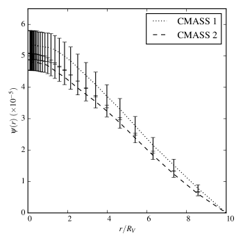
Figure 3.— Lensing potential from Planck data where voids are detected with SDSS data.

From the void profiles shown in the left panel of Figure. 4 and the void parameters in Table. 1, if we calculate the excess mass $\delta m=4\pi\int_{0}^{\infty}\delta_{V}(x)*x^{2}\mbox{d}x$, we could see that the excess mass lies within the range $(-2.5,-1.5)$ for Model A and $(-1.5,-0.5)$ for Model B. The range of value indicates that voids found in SDSS data are mostly undercompensated, having less density than the average. This indicates the fact that voids in underdense regions are easily found with high significant levels in SDSS data since large voids are usually found in underdense regions. We also notice that without $\gamma_{V}$ the excess mass is higher in the negative value.

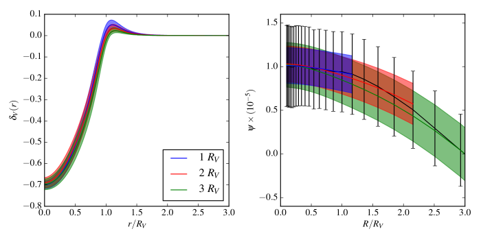
Figure 4.— Best-fit void profiles and lensing potentials for each dataset. The blue, red, and green bands are for Data-I, Data-II, and Data-III respectively. All the error bars are $1\,\sigma$ for cmass1 sample.

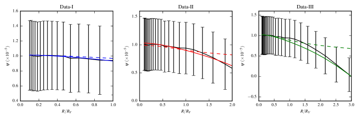
Figure 5.— Best-fit lensing potential for Data-I, Data-II, and Data-III (left to right). The solid lines are void parameter with the environment parameter while the dashed lines are void parameters without the environment parameter. Even though all the models with the environment parameter fit better with the data, the model without the environment parameter also fits well for Data-I and Data-II. All the plots are subjected to the condition $\psi(r=3R_{V})=0$. The error bars are $1\,\sigma$.

In Table. 1, we show the best-fit parameters within $1\,\sigma$ uncertainties. The parameters from different datasets are all agree within the uncertainty ranges. The values of the environment parameter $\gamma_{V}$ are approximately $\sim-0.08$ for cmass1 and $\sim-0.05$ for cmass2 with a high significant detection level from zero. The negative value of $\gamma_{V}$ indicates that on average the voids in SDSS data are in a locally underdense region, which is also confirmed by the integrated mass discussed previously. This effect could be seen from the lensing potential shown in Figure. 3. Since the deflection angle is equal to the gradient of the lensing potential $(\boldsymbol{\alpha}\equiv\boldsymbol{\nabla}_{\perp}\psi)$, the nonzero gradient of the lensing potential at large radius indicates that there is some residue lensing power. The lensing power mainly comes from the deficit (or excess) mass from the voids (or clusters). The constancy of the gradient translates into the constancy of the excess mass. Our MCMC has shown that this residue power is caused by the mass deficit by having a negative value of $\gamma_{V}$. However, this comes with the caveat, as stated in Planck Collaboration et al. (2016d), that the lensing potential has a very red spectrum and when cutting the map into small regions it could cause a leakage issue. This is the reason the team chose to release the lensing convergence rather than the potential. And for our purposes we need to convert it back to the lensing potential (§2.1).

To justify the necessity of the environment parameter, the best-fit lensing potentials from the models with and without the environment parameter are shown in Figure. 5. The likelihood ratios between the models with and without the environment parameter $\mathcal{L}_{\text{w}}/\mathcal{L}_{\text{w/o}}$ are 1.01, 1.36, and 77.4 for Data-I, Data-II, and Data-III, respectively, for cmass1. Without taking the penalty of an additional parameter in $\mathcal{L}_{\text{w}}$ into account, we could see that the environment parameter is preferred in Data-III, while it is less preferable for Data-I and Data-II. The best-fit parameters for all samples and models are shown in Table. 1. From Table. 1, the significant detection levels for the environment parameter for Data-I, Data-II and Data-III are approximately $15\sigma$, $30\,\sigma$, and $47\,\sigma$ for Data-I, Data-II, and, Data-III, respectively, for the cmass1 sample respectively. The general results hold similarly for the cmass2 sample.

To analyze the effect of $\gamma_{V}$ on the other parameters, we shall take to the best-fit parameters from Data-III for the cmass1 sample from Table. 1 for a comparison. The effects of how the HSW parameters alter the shape of the void profile are explicitly shown in Figure. 8 in Barreira et al. (2015). In both models, the values of $\beta$ between the two models are not much different given the uncertainties in the values—the values differ by $2.3\,\sigma$. The similarity in the values of $\beta$ indicates that the extensions of the compensation region are similar. However, the values of $\alpha$, $\delta_{c}$, and $R_{S}/R_{V}$ are significantly different by $4.4\,\sigma$, $3.6\,\sigma$, and $6.6\,\sigma$, respectively. $\alpha$ describes the slope of the underdense region, $\delta_{c}$ describes the depth of the void profile, and $R_{S}/R_{V}$ is the zero-crossing radius. In general, Model B (with $\gamma_{V}$) gives a shallower void profile than the Model A (without $\gamma_{V}$) by having smaller values of $\alpha$ and $\delta_{c}$. This indicates that $\gamma_{V}$ has a direct degenerate effect with both $\alpha$ and $\delta_{c}$—lowering the mean density could be compensated by having a shallower profile.

Attempts to recover or fit the HSW void parameters are found in Nadathur et al. (2016, hereafter, N14) and Hamaus et al. (2015, hereafter, H15). In N14, the stacked void profiles for different radii and redshifts are compared between a mock luminous red galaxy (LRG) catalog from the Jubilee simulation and the SDSS LRG and Main Galaxy samples. They have found that the void profiles from the simulations and the SDSS galaxy samples matched. H15 investigated the redshift-space distortions between pairs of galaxies from a mock galaxies catalog with HOD parameters from Zheng et al. (2007) and Manera et al. (2013) and stacked voids in redshift space. The inference on the HSW void parameters was made by assuming the Gaussian streaming model, where the distribution of the pairwise line-of-sight velocities is assumed to be Gaussian. The HSW parameters in N14 and H15 are $(\alpha,\beta,\delta_{c},R_{S}/R_{V})=(1.57,5.72,-0.69,0.81)$ and $(\alpha,\beta,\delta_{c})=(0.96\leavevmode\nobreak\ \pm\leavevmode\nobreak\ 0.14,8.84\leavevmode\nobreak\ \pm\leavevmode\nobreak\ 1.16,-0.912\leavevmode\nobreak\ \pm\leavevmode\nobreak\ 0.052)$ respectively. The main differences in the parameter constraints from our work and theirs are from the different methodology used in deriving the parameters and the inclusion of $\gamma_{V}$. We also notice that the value of $\delta_{c}$ between N14 (observationally derived) and our value, especially for Data-I, are similar, while the value of $\delta_{c}$ from H15 (mock catalog derived) is remarkably different. This may indicate a systematic bias between the SDSS samples and the mock catalog.

To summarize this work, we cross-correlated the Planck lensing map with 516 voids found in the SDSS data and stacked them to obtain the stacked lensing potential from voids. From the stacked void lensing potential, we recover the HSW void parameter from three different data sets: Data-I to $1R_{V}$, Data-II to $2R_{V}$, and Data-III to $3R_{V}$. We have found that it is necessary to include the environment parameter in the void profile to obtain a good fit to the data. The environment parameter has a physical interpretation that voids found in the SDSS data are mostly undercompensated voids and reside within an underdense region. The effects of the deficit mass are shown in Figure. 3, where the gradient of the lensing potential is constant at large distances.

References

- Abazajian et al. (2009) Abazajian, K. N., Adelman-McCarthy, J. K., Agüeros, M. A., et al. 2009, ApJS, 182, 543
- Ahn et al. (2014) Ahn, C. P., Alexandroff, R., Allende Prieto, C., et al. 2014, ApJS, 211, 17
- Alcock & Paczynski (1979) Alcock, C., & Paczynski, B. 1979, Nature, 281, 358
- Andrieu & Thoms (2008) Andrieu, C., & Thoms, J. 2008, Statistics and Computing, 18, 343
- Barreira et al. (2015) Barreira, A., Cautun, M., Li, B., Baugh, C. M., & Pascoli, S. 2015, JCAP, 8, 028
- Bartelmann & Schneider (2001) Bartelmann, M., & Schneider, P. 2001, Phys. Rep., 340, 291
- Beygu et al. (2013) Beygu, B., Kreckel, K., van de Weygaert, R., van der Hulst, J. M., & van Gorkom, J. H. 2013, AJ, 145, 120
- Biswas et al. (2010) Biswas, R., Alizadeh, E., & Wandelt, B. D. 2010, Phys. Rev. D, 82, 023002
- Bolejko et al. (2013) Bolejko, K., Clarkson, C., Maartens, R., et al. 2013, Physical Review Letters, 110, 021302
- Bos et al. (2012) Bos, E. G. P., van de Weygaert, R., Dolag, K., & Pettorino, V. 2012, MNRAS, 426, 440
- Boylan-Kolchin et al. (2009) Boylan-Kolchin, M., Springel, V., White, S. D. M., Jenkins, A., & Lemson, G. 2009, MNRAS, 398, 1150
- Cai et al. (2014) Cai, Y.-C., Neyrinck, M. C., Szapudi, I., Cole, S., & Frenk, C. S. 2014, ApJ, 786, 110
- Cai et al. (2015) Cai, Y.-C., Padilla, N., & Li, B. 2015, MNRAS, 451, 1036
- Ceccarelli et al. (2006) Ceccarelli, L., Padilla, N. D., Valotto, C., & Lambas, D. G. 2006, MNRAS, 373, 1440
- Chantavat et al. (2016) Chantavat, T., Sawangwit, U., Sutter, P. M., & Wandelt, B. D. 2016, Phys. Rev. D, 93, 043523
- Chen & Kantowski (2015) Chen, B., & Kantowski, R. 2015, Phys. Rev. D, 91, 083014
- Chen et al. (2015) Chen, B., Kantowski, R., & Dai, X. 2015, ApJ, 804, 130
- Clampitt et al. (2013) Clampitt, J., Cai, Y.-C., & Li, B. 2013, MNRAS, 431, 749
- Clampitt & Jain (2015) Clampitt, J., & Jain, B. 2015, MNRAS, 454, 3357
- Courtois et al. (2012) Courtois, H. M., Hoffman, Y., Tully, R. B., & Gottlöber, S. 2012, ApJ, 744, 43
- Das & Spergel (2009) Das, S., & Spergel, D. N. 2009, Phys. Rev. D, 79, 043007
- Einstein (1936) Einstein, A. 1936, Science, 84, 506
- Górski et al. (2005) Górski, K. M., , & et al. 2005, ApJ, 622, 759
- Granett et al. (2008) Granett, B. R., Neyrinck, M. C., & Szapudi, I. 2008, ApJL, 683, L99
- Gruen et al. (2016) Gruen, D., Friedrich, O., Amara, A., et al. 2016, MNRAS, 455, 3367
- Hald (1999) Hald, A. 1999, Statist. Sci., 14, 214
- Hamaus et al. (2015) Hamaus, N., Sutter, P. M., Lavaux, G., & Wandelt, B. D. 2015, JCAP, 11, 036
- Hamaus et al. (2014a) Hamaus, N., Sutter, P. M., & Wandelt, B. D. 2014a, Physical Review Letters, 112, 251302
- Hamaus et al. (2014b) Hamaus, N., Wandelt, B. D., Sutter, P. M., Lavaux, G., & Warren, M. S. 2014b, Physical Review Letters, 112, 041304
- Hastings (1970) Hastings, W. K. 1970, Biometrika, 57, 97
- Higuchi et al. (2013) Higuchi, Y., Oguri, M., & Hamana, T. 2013, MNRAS, 432, 1021
- Hinshaw et al. (2013) Hinshaw, G., Larson, D., Komatsu, E., et al. 2013, ApJS, 208, 19
- Hotchkiss et al. (2015) Hotchkiss, S., Nadathur, S., Gottlöber, S., et al. 2015, MNRAS, 446, 1321
- Ilić et al. (2013) Ilić, S., Langer, M., & Douspis, M. 2013, A&A, 556, A51
- Jennings et al. (2013) Jennings, E., Li, Y., & Hu, W. 2013, MNRAS, 434, 2167
- Kaiser (1987) Kaiser, N. 1987, MNRAS, 227, 1
- Krause et al. (2013) Krause, E., Chang, T.-C., Doré, O., & Umetsu, K. 2013, ApJL, 762, L20
- Lavaux & Wandelt (2012) Lavaux, G., & Wandelt, B. D. 2012, ApJ, 754, 109
- Lee & Park (2009) Lee, J., & Park, D. 2009, ApJL, 696, L10
- Manera et al. (2013) Manera, M., Scoccimarro, R., Percival, W. J., et al. 2013, MNRAS, 428, 1036
- Melchior et al. (2014) Melchior, P., Sutter, P. M., Sheldon, E. S., Krause, E., & Wandelt, B. D. 2014, MNRAS, 440, 2922
- Metropolis et al. (1953) Metropolis, N., Rosenbluth, A. W., Rosenbluth, M. N., Teller, A. H., & Teller, E. 1953, J. Chem. Phys., 21, 1087
- Nadathur (2016) Nadathur, S. 2016, MNRAS, 461, 358
- Nadathur et al. (2016) Nadathur, S., Hotchkiss, S., Diego, J. M., et al. 2016, in IAU Symposium, Vol. 308, The Zeldovich Universe: Genesis and Growth of the Cosmic Web, ed. R. van de Weygaert, S. Shandarin, E. Saar, & J. Einasto, 542–545
- Neyrinck (2008) Neyrinck, M. C. 2008, MNRAS, 386, 2101
- Okamoto & Hu (2003) Okamoto, T., & Hu, W. 2003, Phys. Rev. D, 67, 083002
- Pan et al. (2012) Pan, D. C., Vogeley, M. S., Hoyle, F., Choi, Y.-Y., & Park, C. 2012, MNRAS, 421, 926
- Penny et al. (2015) Penny, S. J., Brown, M. J. I., Pimbblet, K. A., et al. 2015, MNRAS, 453, 3519
- Planck Collaboration et al. (2014) Planck Collaboration, Ade, P. A. R., Aghanim, N., et al. 2014, A&A, 571, A16
- Planck Collaboration et al. (2016a) Planck Collaboration, Adam, R., Ade, P. A. R., et al. 2016a, A&A, 594, A1
- Planck Collaboration et al. (2016b) —. 2016b, A&A, 594, A9
- Planck Collaboration et al. (2016c) Planck Collaboration, Ade, P. A. R., Aghanim, N., et al. 2016c, A&A, 594, A13
- Planck Collaboration et al. (2016d) —. 2016d, A&A, 594, A15
- Planck Collaboration et al. (2016e) —. 2016e, A&A, 594, A21
- Platen et al. (2007) Platen, E., van de Weygaert, R., & Jones, B. J. T. 2007, MNRAS, 380, 551
- Press et al. (2007) Press, W. H., Teukolsky, S. A., Vetterling, W. T., & Flannery, B. P. 2007, Numerical Recipes: The Art of Scientific Computing, 3rd edn. (New York, NY, USA: Cambridge University Press)
- Roberts & Rosenthal (2007) Roberts, G. O., & Rosenthal, J. S. 2007, Journal of Applied Probability, 44, 458
- Sachs & Wolfe (1967) Sachs, R. K., & Wolfe, A. M. 1967, ApJ, 147, 73
- Sheth & van de Weygaert (2004) Sheth, R. K., & van de Weygaert, R. 2004, MNRAS, 350, 517
- Sutter et al. (2012a) Sutter, P. M., Lavaux, G., Wandelt, B. D., & Weinberg, D. H. 2012a, ApJ, 761, 187
- Sutter et al. (2012b) —. 2012b, ApJ, 761, 44
- Sutter et al. (2014a) Sutter, P. M., Lavaux, G., Wandelt, B. D., et al. 2014a, MNRAS, 442, 3127
- Sutter et al. (2014b) Sutter, P. M., Pisani, A., Wandelt, B. D., & Weinberg, D. H. 2014b, MNRAS, 443, 2983
- Zheng et al. (2007) Zheng, Z., Coil, A. L., & Zehavi, I. 2007, ApJ, 667, 760
- Zivick et al. (2015) Zivick, P., Sutter, P. M., Wandelt, B. D., Li, B., & Lam, T. Y. 2015, MNRAS, 451, 4215