Nucleon electromagnetic and axial form factors with N${}_{\textrm{f}}$=2 twisted mass fermions at the physical point

Abstract:

We present results for the nucleon electromagnetic and axial form factors using an N${}_{\textrm{f}}$=2 twisted mass fermion ensemble with pion mass of about 131 MeV. We use multiple sink-source separations to identify excited state contamination. Dipole masses for the momentum dependence of the form factors are extracted and compared to experiment, as is the nucleon magnetic moment and charge and magnetic radii.

1 Introduction

Form factors of the nucleon are fundamental probes of its structure. The electromagnetic form factors are related to the nucleon magnetic moment, its electric and magnetic radii. Axial form factors probe chiral symmetry and test partial conservation of the axial current (PCAC), having been studied in chiral effective theories.

Both electromagnetic and axial form factors have been extensively studied in lattice QCD. Recent experimental results, in combination with availability of simulations with physical quark masses on the lattice, have increased interest in an ab initio calculation of these form factors. These include tension between the value obtained for the proton radius between electron scattering [1] and hydrogen spectroscopy [2] as well as with recent measurements of muonic deuterium spectroscopy [3]. Furthermore recent re-analyses of neutrino scattering data [4, 5] report large systematics in the determination of the axial dipole mass $M_{A}$. In this contribution, we calculate the axial and electromagnetic form factors of the nucleon on an ensemble of twisted mass fermion configurations with clover improvement and two degenerate light quarks (N${}_{\textrm{f}}=2$) tuned to reproduce a pion mass of about 131 MeV [6]. We use multiple sink-source separations and $\mathcal{O}(10^{5})$ statistics to evaluate excited state effects in these quantities.

2 Setup and lattice parameters

2.1 Axial and Electromagnetic form factors

Form factors are extracted from nucleon matrix elements:

$$\langle N(p^{\prime},s^{\prime})|\mathcal{O}^{X}_{\mu}|N(p,s)\rangle=\sqrt{\frac{m^{2}_{N}}{E_{N}(\vec{p}^{\prime})E_{N}(\vec{p})}}\bar{u}_{N}(p^{\prime},s^{\prime})\Lambda^{X}_{\mu}(q^{2})u_{N}(p,s)$$

with $N(p,s)$ a nucleon state of momentum $p$ and spin $s$, $E_{N}(\vec{p})=p_{0}$ its energy and $m_{N}$ its mass, $q=p^{\prime}-p$, the momentum transfer from initial ($p$) to final ($p^{\prime}$) momentum, $u_{N}$ a nucleon spinor and $\mathcal{O}^{X}$ either the axial ($X=A$) or vector $(X=V)$ current. For the case of axial form factors, we use the axial current: $\mathcal{O}^{A}_{\mu}$ = $A^{3}_{\mu}$ = $\bar{\psi}\frac{\tau_{3}}{2}\gamma_{5}\gamma_{\mu}\psi$, with $\bar{\psi}=(\bar{u},\bar{d})$, $u$ and $d$ up- and down-quark fields and $\tau_{3}$ the third Pauli matrix acting on flavor space. For the electromagnetic form factors we use the isovector, symmetrized lattice conserved vector current $\mathcal{O}^{V}_{\mu}$ = $\frac{1}{2}[j_{\mu}(x)+j_{\mu}(x-\hat{\mu})]$, with $j_{\mu}(x)$ the Wilson conserved current. Use of the isovector current means that disconnected contributions cancel. Furthermore, use of the conserved electromagnetic current means no renormalization of the vector operator is required. For the axial form factors we use $Z_{A}=$0.7910(4)(5) [7]. The matrix element of the axial current yields the axial $G_{A}$ and induced pseudo-scalar $G_{p}$ form factors, while the vector current yields the Dirac $F_{1}$ and Pauli $F_{2}$ form factors:

$$\Lambda^{A}_{\mu}(q^{2})=\frac{i}{2}\gamma_{5}\gamma_{\mu}G_{A}(q^{2})+\frac{q_{\mu}\gamma_{5}}{2m_{N}}G_{p}(q^{2}),\quad\Lambda_{\mu}^{V}(q^{2})=\gamma_{\mu}F_{1}(q^{2})+\frac{i\sigma_{\mu\nu}q^{\nu}}{2m_{N}}F_{2}(q^{2}).$$ (1)

The Dirac and Pauli form factors can also be expressed in terms of the nucleon electric $G_{E}$ and magnetic $G_{M}$ Sachs form factors via $G_{E}(q^{2})=F_{1}(q^{2})+\frac{q^{2}}{(2m_{N})^{2}}F_{2}(q^{2})$ and $G_{M}(q^{2})=F_{1}(q^{2})+F_{2}(q^{2})$.

2.2 Lattice extraction of form factors

On the lattice, extraction of matrix elements requires calculating a three-point correlation function. We use sequential inversions through the sink fixing the sink momentum $\vec{p}^{\prime}$ to zero, which constrains $\vec{p}=-\vec{q}$. We form a ratio of three- to two-point functions which, after taking the large time limit, cancel unknown overlaps and energy exponentials: $R_{\mu}(\Gamma;\vec{q};t_{s};t_{\rm ins})\xrightarrow[t_{\rm ins}\gg]{t_{s}-t_{\rm ins}\gg}\Pi_{\mu}(\Gamma;\vec{q})$, where $R_{\mu}$ is the ratio of three- to two-point functions as defined in Ref. [8], $t_{s}$ ($t_{\textrm{ins}}$) the sink (insertion) time assuming the source is at the origin, and $\Gamma$ the sink polarization.

In what follows we will use two methods to extract $\Pi_{\mu}$ from lattice data: i) in the standard plateau method, we fit the $t_{\rm ins}$ dependence of $\Pi_{\mu}$ to a constant for multiple $t_{s}$ values observing the dependence with $t_{s}$, as shown for $G_{E}$ in the left panel of Fig. 1. Excited states are suppressed when our result does not change with $t_{s}$. ii) in the summation method, we calculate: $\sum_{t_{\rm ins}}R_{\mu}(\Gamma;\vec{q};t_{s};t_{\rm ins})\xrightarrow{t_{s}\gg}\Pi_{\mu}(\Gamma;\vec{q})t_{s}+C$ and carry out a two-parameter fit for obtaining the slope, as in the right panel of Fig. 1.

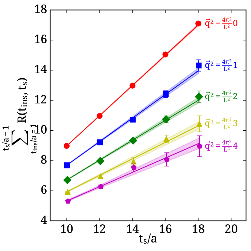
Figure 1: Example fits for $G_{E}$, left for the plateau method for three lattice momenta, and right for the summation method for the first five lattice momenta. On the left, with the grey bands, we also show the result of the summation method.

Having $\Pi_{\mu}(\Gamma;\vec{q})$, different combinations of current insertion directions ($\mu$) and nucleon polarizations determined by $\Gamma$ yield different form factors. Using $\Pi^{V}$ to denote electromagnetic and $\Pi^{A}$ for axial matrix elements, we have:

$$\Pi^{V}_{0}(\Gamma_{0};\vec{q})= \mathcal{C}\frac{E_{N}+m_{N}}{2m_{N}}G_{E}(Q^{2}),\quad \Pi^{V}_{i}(\Gamma_{0};\vec{q})= \mathcal{C}\frac{q_{i}}{2m_{N}}G_{E}(Q^{2})$$ (2)

$$\Pi^{V}_{i}(\Gamma_{k};\vec{q})= \mathcal{C}\frac{\epsilon_{ijk}q_{j}}{2m_{N}}G_{M}(Q^{2}),\quad \Pi^{A}_{i}(\Gamma_{k};\vec{q})= \frac{i\mathcal{C}}{4m_{N}}[\frac{q_{k}q_{i}}{2m_{N}}G_{p}(Q^{2})-(E_{N}+m_{N})\delta_{ik}G_{A}(Q^{2})]$$

where $Q^{2}=-q^{2}$, $\mathcal{C}=\sqrt{\frac{2m_{N}^{2}}{E_{N}(E_{N}+m_{N})}}$, the unpolarized projector: $\Gamma_{0}=\frac{1+\gamma_{0}}{4}$, the polarized projector: $\Gamma_{k}=i\gamma_{5}\gamma_{k}\Gamma_{0}$, and $i,k=1,2,3$.

2.3 Lattice setup

We use a lattice with volume 48${}^{3}\times$96 and lattice spacing determined at a $\simeq$ 0.093 fm [9]. The parameters of the calculation are summarized in Table 1. This setup allows calculation of $G_{E}$ on all five sink-source separations and of $G_{M}$, $G_{A}$ and $G_{p}$ on the three smallest. $G_{E}$ and $G_{M}$ can be extracted directly via Eq. (2) since they depend on different sink projectors. $G_{A}$ and $G_{p}$ are both extracted from the last expression of Eq. (2). We separate the two form factors via an over-constrained fit, solving the resulting eigenvalue problem via singular value decomposition, as explained in Ref. [10].

$t_{s}$ [a]	Proj.	$N_{\rm cnf}\cdot N_{\rm src}$ =	$N_{\rm st}$
10,12,14	$\Gamma_{0}$, $\Gamma_{k}$	578$\times$16 =	9248
16	$\Gamma_{0}$	530$\times$88 =	46640
18	$\Gamma_{0}$	725$\times$88 =	63800

Table 1: Form factor calculation setup. The first column shows the sink-source separations used, the second column the sink projectors and the last column the total statistics ($N_{\rm st}$) obtained using $N_{\rm cnf}$ configurations times $N_{\rm src}$ source-positions per configuration.

3 Results

3.1 Axial form factors

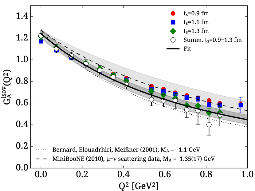
Figure 2: Left: Axial nucleon form factor using $t_{s}\simeq$ 0.9 fm (red circles), 1.1 fm (blue squares), and 1.3 fm (green diamonds) and using the summation method (open circles). The solid line (upper panel) is a fit of the latter to a dipole form. The dashed and dotted lines are from Refs. [4] and [11] respectively. Dipole fit results (lower panel) are compared with $g_{A}$ from Ref. [12] shown with the solid line. Top: Results for the induced pseudo-scalar form factor $G_{p}$ with the notation of the left panel.

The axial form factors are shown in Fig. 2. For $G_{A}$ we see values increasing at low $Q^{2}$ as the sink-source separation increases, while at larger momenta we see a decreasing trend. We fit all three sink-source separations, and the summation method, to a dipole form: $G_{A}(Q^{2})=\frac{g_{A}}{(1+Q^{2}/M_{A}^{2})^{2}}$, allowing both the axial charge $g_{A}$ and the axial mass $M_{A}$ to vary. We observe $g_{A}$ approaching its experimental value with increasing sink-source separation. More details on this calculation of $g_{A}$ can be found in Ref. [13] in these proceedings. $M_{A}$ is found consistent within errors of a recent experimental determination [4] shown with the dashed line in the central panel of Fig. 2. We note that our values of $M_{A}$ are also consistent within the wide error of a recent reanalysis of experimental data, not shown in Fig. 2, which yields $M_{A}$=1.01(24) GeV [5].

The induced pseudo-scalar form factor $G_{p}$ exhibits similar excited-state dependence at low $Q^{2}$. Assuming a pion-pole motivates the form: $G_{p}(Q^{2})=G_{A}(Q^{2})C/(1+\frac{Q^{2}}{m_{\pi}^{2}})$ to which we fit to using a dipole form for $G_{A}$ thus requiring only $C$ to vary. We obtain $\sqrt{C}/2=5.9(2)$ to be compared to the phenomenological expectation $\sqrt{C}/2=m_{N}/m_{\pi}=7.16(4)$ [10].

3.2 Electromagnetic form factors

The isovector electromagnetic Sachs form factors are shown in Fig. 3, where for $G_{E}$ two additional $t_{s}$ values are available. For $G_{E}$ we see a tendency towards the experimental results as $t_{s}$ increases. The same is not observed for $G_{M}$ which underestimates the low-$Q^{2}$ experimental values and which decreases with increasing $t_{s}$.

Figure 3: Isovector electric (left) and magnetic (right) Sachs form factors. For $G_{E}$ we show with yellow triangles and magenta pentagons $t_{s}\simeq$ 1.5 and 1.7 fm respectively. Asterisks denote the summation method. The solid line and band denotes fits to a dipole form as explained in the text. The dashed line is the experimental parameterization.

The electric and magnetic radii are related to the slope of the form factors at $Q^{2}=0$, namely: $\langle r^{2}_{i}\rangle=-\frac{6}{G_{i}(0)}\partial G_{i}(Q^{2})/\partial Q^{2}$, $i=E,M$. We fit all sink-source separations and the summation method to a dipole form $G_{i}(Q^{2})=G_{i}(0)/(1+\frac{Q^{2}}{M_{i}^{2}})^{2}$ with $\langle r^{2}_{i}\rangle=\frac{12}{M^{2}_{i}}$. For $G_{E}$ we fix $G_{E}(0)=1$ while for $G_{M}$ we allow $G_{M}(0)$ to vary. The results are shown in Fig. 4 where for both electric and magnetic radii we see an increasing trend towards the experimentally determined values as $t_{s}$ increases, while $G_{M}(0)$ shows mild dependence on $t_{s}$.

Figure 4: Results for isovector $\langle r_{E}^{2}\rangle$ (left) and $\langle r_{M}^{2}\rangle$ (bottom right) and $G_{M}(0)$ (top right) from dipole fits. Fits to results using the plateau method are shown with the symbol notation of Fig. 3. For the summation method we fit all available $t_{s}$ to obtain the filled asterisk and starting from 1.1 fm using the open asterisk. The open circles are the experimental result from Ref. [1] while the open square from Ref. [2].

Our results for the isovector electric and magnetic charge radii are compared to those of other recent lattice calculations in Fig. 5. We see that for both radii lattice results agree within errors and are within at most 2-$\sigma$ to the experimental values. With further improvement on systematic uncertainties and with increased statistics, contacting experiment is within reach for these quantities.

4 Summary and conclusions

The isovector axial and electromagnetic form factors of the nucleon have been calculated on a lattice with physical pion mass at multiple sink-source separations up to $\sim$1.7 fm and for $\mathcal{O}(10^{5})$ statistics. We find that excited states increase the axial mass and at separations beyond 1.3 fm our result agrees with experimental measurements.

Figure 5: Our results for the isovector $\langle r_{E}^{2}\rangle$ (left) and $\langle r_{M}^{2}\rangle$ (center), shown with blue squares using the plateau method for the largest $t_{s}$ in each case. The smaller error-bar indicates the statistical error while the larger error includes the systematic uncertainty when considering the summation method. We compare to recent lattice calculations: PNDME [14] (green diamonds), Mainz [15] (magenta pentagons) and LHPC [16] (red circles). The vertical lines show the experimental values also shown in Fig. 4. In the right panel we show a preliminary result of using the position space method of Ref. [17] for determining the slope of $G_{E}(Q^{2})$ for the separation $t_{s}\simeq$1.7 fm.

The electric and magnetic charge radii show similar behavior, approaching the experimental values with increasing $t_{s}$. For $G_{M}(0)$, the value at $Q^{2}=0$ is underestimated with mild excited state dependence. Calculations at a larger volume, with access to finer momenta, are being carried out to asses the effect on $G_{M}(0)$.

Recent methods for fitting form factors with no model assumption of the their $Q^{2}$ dependence allow for further assessment of systematic uncertainties. In the right panel of Fig. 5 we show the result of applying the position space method of Ref. [17], originally applied for $G_{M}(0)$, to obtain $\langle r^{2}_{E}\rangle$ at $t_{s}=1.7$ fm. At all separations we obtain results for $\langle r^{2}_{E}\rangle$ consistent with what is obtained by the dipole fits shown in Fig. 4. Such methods can benefit from finer momenta using larger lattice volumes, as well as from reduced errors at larger $Q^{2}$ using appropriate momentum-dependent smearing as in Ref. [18], both avenues which are currently being explored.

Acknowledgments: Results were obtained using Jureca, via NIC allocation ECY00, HazelHen at HLRS and SuperMUC at LRZ via Gauss allocations with ids 44066 and 10862 and Piz Daint at CSCS via projects with ids s540 and s625. We thank the staff of these centers for access to the computational resources and for their support.

References

• [1] P. J. Mohr, D. B. Newell, and B. N. Taylor, Rev. Mod. Phys. 88, 035009 (2016), 1507.07956.
• [2] R. Pohl et al., Nature 466, 213 (2010).
• [3] R. Pohl et al., Science 353, 669 (2016).
• [4] MiniBooNE, A. A. Aguilar-Arevalo et al., Phys. Rev. D81, 092005 (2010), 1002.2680.
• [5] A. S. Meyer, M. Betancourt, R. Gran, and R. J. Hill, Phys. Rev. D93, 113015 (2016), 1603.03048.
• [6] ETM, A. Abdel-Rehim et al., (2015), 1507.05068.
• [7] A. Abdel-Rehim et al., Phys. Rev. D (in press) (2015), 1507.04936.
• [8] ETM, C. Alexandrou et al., Phys. Rev. D83, 045010 (2011), 1012.0857.
• [9] ETM, A. Abdel-Rehim et al., Phys. Rev. Lett. 116, 252001 (2016), 1601.01624.
• [10] C. Alexandrou, G. Koutsou, T. Leontiou, J. W. Negele, and A. Tsapalis, Phys. Rev. D76, 094511 (2007), 0706.3011, [Erratum: Phys. Rev.D80,099901(2009)].
• [11] V. Bernard, L. Elouadrhiri, and U.-G. Meissner, J. Phys. G28, R1 (2002), hep-ph/0107088.
• [12] C. Patrignani, Chin. Phys. C40, 100001 (2016).
• [13] C. Alexandrou et al., PoS LATTICE2016, 153 (2016).
• [14] T. Bhattacharya et al., Phys. Rev. D89, 094502 (2014), 1306.5435.
• [15] S. Capitani et al., Phys. Rev. D92, 054511 (2015), 1504.04628.
• [16] J. Green et al., Phys.Rev. D90, 074507 (2014), 1404.4029.
• [17] ETM, C. Alexandrou, M. Constantinou, G. Koutsou, K. Ottnad, and M. Petschlies, (2016), 1605.07327.
• [18] G. S. Bali, B. Lang, B. U. Musch, and A. Schäfer, Phys. Rev. D93, 094515 (2016), 1602.05525.