Deep Learning with Low Precision by Half-wave Gaussian Quantization
Abstract
The problem of quantizing the activations of a deep neural network is considered. An examination of the popular binary quantization approach shows that this consists of approximating a classical non-linearity, the hyperbolic tangent, by two functions: a piecewise constant function, which is used in feedforward network computations, and a piecewise linear hard tanh function, used in the backpropagation step during network learning. The problem of approximating the ReLU non-linearity, widely used in the recent deep learning literature, is then considered. An half-wave Gaussian quantizer (HWGQ) is proposed for forward approximation and shown to have efficient implementation, by exploiting the statistics of of network activations and batch normalization operations commonly used in the literature. To overcome the problem of gradient mismatch, due to the use of different forward and backward approximations, several piece-wise backward approximators are then investigated. The implementation of the resulting quantized network, denoted as HWGQ-Net, is shown to achieve much closer performance to full precision networks, such as AlexNet, ResNet, GoogLeNet and VGG-Net, than previously available low-precision networks, with 1-bit binary weights and 2-bit quantized activations.
1 Introduction
Deep neural networks have achieved state-of-the-art performance on computer vision problems, such as classification [22, 36, 37, 12, 13], detection [7, 33, 1], etc. However, their complexity is an impediment to widespread deployment in many applications of real world interest, where either memory or computational resource is limited. This is due to two main issues: large model sizes (50MB for GoogLeNet [37], 200M for ResNet-101 [13], 250MB for AlexNet [22], or 500M for VGG-Net [36]) and large computational cost, typically requiring GPU-based implementations. This generated interest in compressed models with smaller memory footprints and computation.
Several works have addressed the reduction of model size, through the use of quantization [3, 28, 26], low-rank matrix factorization [19, 6], pruning [11, 10], architecture design [27, 17], etc. Recently, it has been shown that weight compression by quantization can achieve very large savings in memory, reducing each weight to as little as 1 bit, with a marginal cost in classification accuracy [3, 28]. However, it is less effective along the computational dimension, because the core network operation, implemented by each of its units, is the dot-product between a weight and an activation vector. On the other hand, complementing binary or quantized weights with quantized activations allows the replacement of expensive dot-products by logical and bit-counting operations. Hence, substantial speed ups are possible if, in addition to the weights, the inputs of each unit are binarized or quantized to low-bit.
It appears, however, that the quantization of activations is more difficult than that of weights. For example, [4, 32] have shown that, while it is possible to binarize weights with a marginal cost in model accuracy, additional quantization of activations incurs nontrivial losses for large-scale classification tasks, such as object recognition on ImageNet [35]. The difficulty is that binarization or quantization of activations requires their processing with non-differentiable operators. This creates problems for the gradient descent procedure, the backpropagation algorithm, commonly used to learn deep networks. This algorithm iterates between a feedforward step that computes network outputs and a backpropagation step that computes the gradients required for learning. The difficulty is that binarization or quantization operators have step-wise responses that produce very weak gradient signals during backpropagation, compromising learning efficiency. So far, the problem has been addressed by using continuous approximations of the operator used in the feedforward step to implement the backpropagation step. This, however, creates a mismatch between the model that implements the forward computations and the derivatives used to learn it. In result, the model learned by the backpropagation procedure tends to be sub-optimal.
In this work, we view the quantization operator, used in the feedforward step, and the continuous approximation, used in the backpropagation step, as two functions that approximate the activation function of each network unit. We refer to these as the forward and backward approximation of the activation function. We start by considering the binary quantizer, used in [4, 32], for which these two functions can be seen as a discrete and a continuous approximation of a non-linear activation function, the hyperbolic tangent, frequently used in classical neural networks. This activation is, however, not commonly used in recent deep learning literature, where the ReLU nonlinearity [30, 39, 12] has achieved much greater preponderance. This is exactly because it produces much stronger gradient magnitudes. While the hyperbolic tangent or sigmoid non-linearities are squashing non-linearities and mostly flat, the ReLU is an half-wave rectifier, of linear response to positive inputs. Hence, while the derivatives of the hyperbolic tangent are close to zero almost everywhere, the ReLU has unit derivative along the entire positive range of the axis.
To improve the learning efficiency of quantized networks, we consider the design of forward and backward approximation functions for the ReLU. To discretize its linear component, we propose to use an optimal quantizer. By exploiting the statistics of network activations and batch normalization operations that are commonly used in the literature, we show that this can be done with an half-wave Gaussian quantizer (HWGQ) that requires no learning and is very efficient to compute. While some recent works have attempted similar ideas [4, 32], their design of a quantizer is not sufficient to guarantee good deep learning performance. We address this problem by complementing this design with a study of suitable backward approximation functions that account for the mismatch between the forward model and the back propagated derivatives. This study suggests operations such as linearization, gradient clipping or gradient suppression for the implementation of the backward approximation. We show that a combination of the forward HWGQ with these backward operations produces very efficient low-precision networks, denoted as HWGQ-Net, with much closer performance to continuous models, such as AlexNet [22], ResNet [13], GoogLeNet [37] and VGG-Net [36], than other available low-precision networks in the literature. To the best of our knowledge, this is the first time that a single low-precision algorithm could achieve successes for so many popular networks. According to [32], theoretically HWGQ-Net (1-bit weights and 2-bit activations) has 32 memory and 32 convolutional computation savings. These suggest that the HWGQ-Net can be very useful for the deployment of state-of-the-art neural networks in real world applications.
2 Related Work
The reduction of model size is a popular goal in the deep learning literature, due to its importance for the deployment of high performance neural networks in real word applications. One strategy is to exploit the widely known redundancy of neural network weights [5]. For example, [19, 6] proposed low-rank matrix factorization as a way to decompose a large weight matrix into several separable small matrices. This approach has been shown most successful for fully connected layers. An alternative procedure, known as connection pruning [11, 10], consists of removing unimportant connections of a pre-trained model and retraining. This has been shown to reduce the number of model parameters by an order of magnitude without considerable loss in classification accuracy. Another model compression strategy is to constrain the model architecture itself, e.g. by removing fully connected layers, using convolutional filters of small size, etc. Many state-of-the-art deep networks, such as NIN [27], GoogLeNet [37] and ResNet [13], rely on such design choices. For example, SqueezeNet [17] has been shown to achieve a parameter reduction of 50 times, for accuracy comparable to that of AlexNet. Moreover, hash functions have also been used to compress model size [2].
Another branch of approaches for model compression is weight binarization [3, 32, 4] or quantization [28, 26, 8]. [38] used a fixed-point representation to quantize weights of pre-trained neural networks, so as to speed up testing on CPUs. [8] explored several alternative quantization methods to decrease model size, showing that procedures such as vector quantization, with -means, enable 48 times compression with minimal accuracy loss. [26] proposed a method for fixed-point quantization based on the identification of optimal bit-width allocations across network layers. [24, 28] have shown that ternary weight quantization into levels can achieve or model compression with slight accuracy loss, even on large-scale classification tasks. Finally, [3] has shown that filter weights can be quantized to without noticeable loss of classification accuracy on datasets such as CIFAR-10 [21].
Beyond weight binarization, the quantization of activations has two additional benefits: 1) further speed-ups by replacement of the expensive inner-products at the core of all network computations with logical and bit-counting operations; 2) training memory savings, by avoiding the large amounts of memory required to cache full-precision activations. Due to these, activation quantization has attracted some attention recently [38, 26, 4, 32, 40, 25, 28]. In [38], activations were quantized with 8 bits, to achieve speed-ups on CPUs. By performing the quantization after network training, this work avoided the issues of nondifferentiable optimization. [26] developed an optimal algorithm for bit-width allocation across layers, but did not propose a learning procedure for quantized neural networks. Recently, [4, 32, 40] tried to tackle the optimization of networks with nondifferentiable quantization units, by using a continuous approximation to the quantizer function in the backpropagation step. [25] proposed several potential solutions to the problem of gradient mismatch and [28, 40] showed that gradients can be quantized with a small number of bits during the backpropagation step. While some of these methods have produced good results on datasets such as CIFAR-10, none has produced low precision networks competitive with full-precision models on large-scale classification tasks, such as ImageNet [35].
3 Binary Networks
We start with a brief review of the issues involved in the binarization of a deep network.
3.1 Goals
Deep neural networks are composed by layers of processing units that roughly model the computations of the neurons found in the mammalian brain. Each unit computes an activation function of the form
| (1) |
where is a weight vector, an input vector, and a non-linear function. A convolutional network implements layers of these units, where weights are usually represented as a tensor . The dimensions , and are defined by the number of filter channels, width and height, respectively. Since this basic computation is repeated throughout the network and modern networks have very large numbers of units, the structure of (1) is the main factor in the complexity of the overall model. This complexity can be a problem for applications along two dimensions. The first is the large memory footprint required to store weights w. The second is the computational complexity required to compute large numbers of dot-products . Both difficulties are compounded by the requirement of floating point storage of weights and floating point arithmetic to compute dot-products, which are not practical for many applications. This has motivated interest in low-precision networks [4, 32, 40].
3.2 Weight Binarization
An effective strategy to binarize the weights W of convolutional filters, which we adopt in this work, has been proposed by [32]. This consists of approximating the full precision weight matrix W, used to compute the activations of (1) for all the units, by the product of a binary matrix and a scaling factor , such that . A convolutional operation on input I can then be approximated by
| (2) |
where denotes a multiplication-free convolution. [32] has shown that an optimal approximation can be achieved with and . More details can be found in [32].
While binary weights tremendously reduce the memory footprint of the model, they do not fully solve the problem of computational complexity. Since I consists of either the activations of a previous layer or some transformation of the image to classify, it is usually represented with full precision. Hence, (2) requires floating point arithmetic and produces a floating point result. Substantial further reductions of complexity can be obtained by the binarization of I, which enables the implementation of dot products with logical and bit-counting operations [4, 32].
3.3 Binary Activation Quantization
This problem has been studied in the literature, where the use of binary activations has recently become popular [32, 4, 40]. This is usually implemented by replacing in (1) with the non-linearity
| (3) |
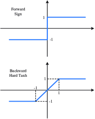
shown in Figure 1. [32] has also considered rescaling the binarized outputs by a factor , but found this to be unnecessary.
While the adoption of (3) greatly simplifies the feedforward computations of the deep model, it severely increases the difficulty of learning. This follows from the fact that the derivative of the sign function is zero almost everywhere. Neural networks are learned by minimizing a cost with respect to the weights . This is done with the backpropagation algorithm, which decomposes these derivatives into a series of simple computations. Consider the unit of (1). The derivative of with respect to is
| (4) |
These derivatives are computed for all units during the backpropagation step. When is replaced by (3), the derivative is zero almost everywhere and the gradient magnitudes tend to be very small. In result, the gradient descent algorithm does not converge to minima of the cost. To overcome this problem, [4] proposed to use an alternative function, hard tanh, which we denote by , in the backpropagation step. This function is shown in Figure 1, and has derivative
| (5) |
In this work, we denote (3) as the forward and (5) as the backward approximations of the activation non-linearity of (1). These approximations have two main problems. The first is that they approximate the hyperbolic tangent
This (and the closely related sigmoid function) is a squashing non-linearity that replicates the saturating behavior of neural firing rates. For this reason, it was widely used in the classical neural net literature. However, squashing non-linearities have been close to abandoned in recent deep learning literature, because the saturating behavior emphasizes the problem of vanishing derivatives, compromising the effectiveness of backpropagation. The second problem is that the discrepancy between the approximation of by the forward and by the backward creates a mismatch between the feedforward model and the derivatives used to learn it. In result, backpropagation can be highly suboptimal. This is called the “gradient mismatch” problem [25].
4 Half-wave Gaussian Quantization
In this section, we propose an alternative quantization strategy, which is based on the approximation of the ReLU non-linearity.
4.1 ReLU
The ReLU is the half-wave rectifier defined by [30]
| (6) |
It is now well known that, when compared to squashing non-linearities, its use in (1) significantly improves the efficiency of the backpropagation algorithm. It thus seems more sensible to rely on ReLU approximations for network quantization than those of the previous section. We propose a quantizer to approximate (6) in the feedforward step and a suitable piecewise linear approximation for the backpropagation step.
4.2 Forward Approximation
A quantizer is a piecewise constant function
| (7) |
that maps all values of within quantization interval into a quantization level , for . In general, and . This generalizes the function, which can be seen as a -bit quantizer. A quantizer is denoted uniform if
| (8) |
where is a constant quantization step. The quantization levels act as the reconstruction values for , under the constraint of reduced precision. Since, for any , it suffices to store the quantization index of (7) to recover the quantization level , non-uniform quantizer requires bits of storage per activation . However, it usually requires more than bits to represent during arithmetic operations, in which it is to be used instead of index . For a uniform quantizer, where is a universal scaling factor that can be placed in evidence, it is intuitive to store any by bits without storing the indexes. The same holds for arithmetic computation.
Optimal quantizers are usually defined in the mean-squared error sense, i.e.
| (9) | ||||
where is the probability density function of . Hence, the optimal quantizer of the dot-products of (1) depends on their statistics. While the optimal solution of (9) is usually non-uniform, a uniform solution is available by adding the uniform constraint of (8) to (9). Given dot product samples, the optimal solution of (9) can be obtained by Lloyd’s algorithm [29], which is similar to -means algorithm. This, however, is an iterative algorithm. Since a different quantizer must be designed per network unit, and this quantizer changes with the backpropagation iteration, the straightforward application of this procedure is computationally intractable.
This difficulty can be avoided by exploiting the statistical structure of the activations of deep networks. For example, [16, 18] have noted that the dot-products of (1) tend to have a symmetric, non-sparse distribution, that is close to Gaussian. Taking into account the fact that ReLU is a half-wave rectifier, this suggests the use of the half-wave Gaussian quantizer (HWGQ),
| (10) |
where for and for ( and ) are the optimal quantization parameters for the Gaussian distribution. The adoption of the HWGQ guarantees that these parameters only depend on the mean and variance of the dot-product distribution. However, because these can vary across units, it does not eliminate the need for the repeated application of Lloyd’s algorithm across the network.
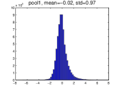
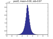
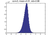
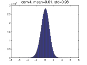
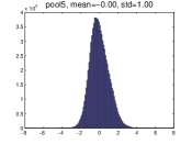
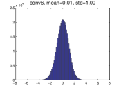
This problem can be alleviated by resorting to batch normalization [18]. This is a widely used normalization technique, which forces the responses of each network layer to have zero mean and unit variance. We apply this normalization to the dot-products, with the result illustrated in Figure 2, for a number of AlexNet units of different layers. Although the distributions are not perfectly Gaussian and there are minor differences between them, they are all close to Gaussian with zero mean and unit variance. It follows that the optimal quantization parameters and are approximately identical across units, layers and backpropagation iterations. Hence, Lloyd’s algorithm can be applied once, with data from the entire network. In fact, because all distributions are approximately Gaussian of zero mean and unit variance, the quantizer can even be designed from samples of this distribution. In our implementation, we drew samples from a standard Gaussian distribution of zero mean and unit variance, and obtained the optimal quantization parameters by Lloyd’s algorithm. The resulting parameters and were used to parametrize a single HWGQ that was used in all layers, after batch normalization of dot-products.
4.3 Backward Approximation
Since the HWGQ is a step-wise constant function, it has zero derivative almost everywhere. Hence, the approximation of by in (4) leads to the problem of vanishing derivatives. As in Section 3, a piecewise linear function can be used during the backpropagation step to avoid weak convergence. In summary, we seek a piece-wise function that provides a good approximation to the ReLU and to the HWGQ. We next consider three possibilities.
4.3.1 Vanilla ReLU
Since the ReLU of (6) is already a piece-wise linear function, it seems sensible to use the ReLU itself, denoted the vanilla ReLU, as the backward approximation function. This corresponds to using the derivative
| (11) |
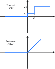
in (4). The forward and backward approximations and of the ReLU are shown in Figure 1. Note that, while the backward approximation is exact, it is not equal to the forward approximation. Hence, there is a gradient mismatch. This mismatch is particularly large for large values of . Note that, for , the approximation of by the ReLU has error . This is usually upper bounded by for but unbounded when . Since these are the values on the tail of the distribution of , the ReLU is said to have a large mismatch with “on the tail.” Due to this, when the ReLU is used to approximate in (4), it can originate very inaccurate gradients for dot-products on the tail of the dot-product distribution. In our experience, these inaccurate gradients can make the learning algorithm unstable.
This is a classical problem in the robust estimation literature, where outliers can unduly influence the performance of a learning algorithm [15]. For quantization, where assumes that values of beyond have very low probability, large dot-products are effectively outliers. The classical solution to mitigate the influence of these outliers is to limit the growth rate of the error function. Since this is , the problem is the monotonicity of the ReLU beyond . To address it, we investigated alternative backwards approximation functions of slower growth rate.

4.3.2 Clipped ReLU
The first approximation, denoted the clipped ReLU, is identical to the vanilla ReLU in but constant beyond ,
| (12) |
Its use to approximate in (4) guarantees that there is no mismatch on the tail. Gradients are non-zero only for dot-products in the interval . We refer to this as ReLU clipping. As illustrated in Figure 3, the clipped ReLU is a better match for the HWGQ than the vanilla ReLU. This idea is similar to the use of gradient clipping in [31]: clipping gradients to enable stable optimization, especially for very deep networks, e.g. recurrent neural network. In our experiments, ReLU clipping is also proved very useful to guarantee stable neural network optimization.
4.3.3 Log-tailed ReLU
Ideally, a network with quantized activations should approach the performance of a full-precision network as the number of quantization levels increases. The sensitivity of the vanilla ReLU approximation to outliers limits the performance of low precision networks (low ). While the clipped ReLU alleviates this problem, it can impair network performance due to the loss of information in the clipped interval . An intermediate solution is to use, in this interval, a function whose growth rate is in between that of the clipped ReLU (zero derivative) and the ReLU (unit derivative). One possibility is to enforce logarithmic growth on the tail, according to
| (13) |
where . This is denoted the log-tailed ReLU and is compared to the ReLU and clipped ReLU in Figure 3. It has derivative
| (14) |
When used to approximate in (4), the log-tailed ReLU is identical to the vanilla ReLU for dot products of amplitude smaller than , but gives decreasing weight to amplitudes larger than this. It behaves like the vanilla ReLU (unit derivative) for but converges to the clipped ReLU (zero derivative) as grows to infinity.
5 Experimental Results
The proposed HWGQ-Net was evaluated on ImageNet (ILSVRC2012) [35], which has 1.2M training images from 1K categories and 50K validation images. The evaluation metrics were top-1 and top-5 classification accuracy. Several popular networks were tested: AlexNet [22], ResNet [13], a variant of VGG-Net [36, 12], and GoogLeNet [37]. Our implementation is based on Caffe [20], and the source code is available at https://github.com/zhaoweicai/hwgq.
5.1 Implementation Details
In all ImageNet experiments, training images were resized to 256256, and a 224224 (227227 for AlexNet) crop was randomly sampled from an image or its horizontal flip. Batch normalization [18] was applied before each quantization layer, as discussed in Section 4.2. Since weight binarization provides regularization constraints, the ratio of dropout [14] was set as 0.1 for networks with binary weights and full activations, but no dropout was used for networks with quantized activations regardless of weight precision. All networks were learned from scratch. No data augmentation was used other than standard random image flipping and cropping. SGD was used for parameter learning. No bias term was used for binarized weights. Similarly to [32], networks with quantized activations used max-pooling before batch normalization, which is denoted “layer re-ordering”. As in [32, 40], the first and last network layers had full precision. Evaluation was based solely on central 224224 crop.
On AlexNet [22] experiments, the mini-batch size was 256, weight decay 0.0005, and learning rate started at 0.01. For ResNet, the parameters were the same as in [13]. For the variant of VGG-Net, denoted VGG-Variant, a smaller version of model-A in [12], only 3 convolutional layers were used for input size of 56, 28 and 14, and the “spp” layer was removed. The mini-batch size was 128, and learning rate started at 0.01. For GoogLeNet [37], the branches for side losses were removed, in the inception layers, max-pooling was removed and the channel number of the “reduce” 11 convolutional layers was increased to that of their following 33 and 55 convolutional layers. Weight decay was 0.0002 and the learning strategy was similar to ResNet [13]. For all networks tested, momentum was 0.9, batch normalization was used, and when mini-batch size was 256 (128), the learning rate was divided by 10 after every 50K (100K) iterations, 160K (320K) in total. Only AlexNet, ResNet-18 and VGG-Variant were explored in the following ablation studies. In all tables and figures, “FW” indicates full-precision weights, “BW” binary weights, and “Full” full-precision weights and activations.
| Full | FW+ | FW+ | BW+ | BW+ | |
|---|---|---|---|---|---|
| Top-1 | 55.7 | 46.7 | 55.7 | 43.9 | 53.9 |
| Top-5 | 79.3 | 71.0 | 79.3 | 68.3 | 77.3 |
5.2 Full-precision Activation Comparison
Before considering the performance of the forward quantized activation functions and , we compared the performance of the continuous (hard tanh) and (ReLU) as activation function. In this case, there is no activation quantization nor forward/backward gradient mismatch. AlexNet results are presented in Table 1, using identical settings for and , for fair comparison. As expected from the discussion of Sections 3 and 4, achieved substantially better performance than , for both FW and BW networks. The fact that these results upper bound the performance achievable when quantization is included suggests that is not a good choice for quantization function. , on the other hand, has a fairly reasonable upper bound.
| Model | Full | BW | FW+ | BW+ | BW+ | |
|---|---|---|---|---|---|---|
| AlexNet | Top-1 | 55.7 | 52.4 | 49.5 | 39.5 | 46.8 |
| Top-5 | 79.3 | 75.9 | 73.7 | 63.6 | 71.0 | |
| ResNet-18 | Top-1 | 66.3 | 61.3 | 37.5 | 42.1 | 33.0 |
| Top-5 | 87.5 | 83.6 | 61.9 | 67.1 | 56.9 | |
| VGG-Variant | Top-1 | 68.6 | 65.5 | 48.3 | 50.1 | 44.1 |
| Top-5 | 88.9 | 86.5 | 72.3 | 74.3 | 68.7 | |
5.3 Low-bit Activation Quantization Results
We next compared the performance achieved by adding the and HWGQ (backward vanilla ReLU) quantizers to the set-up of the previous section. The results of AlexNet, ResNet-18 and VGG-Variant are summarized in Table 2. At first, notice that BW is worse than BW+ of AlexNet in Table 1 due to the impact of the layer re-ordering [32] introduced in Section 5.1. Next, comparing BW to FW+, where the former binarizes weights only and the latter quantizes activations only, we observed that weight binarization causes a minor degradation of accuracy. This is consistent with the findings of [32, 4]. On the other hand, activation quantization leads to a nontrivial loss. This suggests that the latter is a more difficult problem than the former. This observation is not surprising since, unlike weight binarization, the learning of an activation-quantized networks needs to propagate gradients through every nondifferentiable quantization layer.
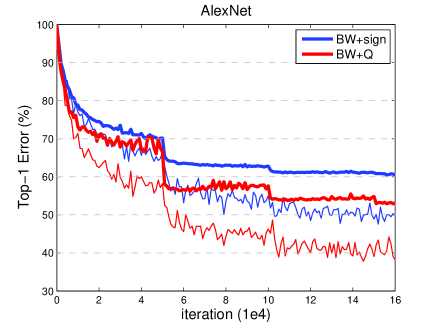
When weight binarization and activation quantization were combined, recognition performance dropped even further. For AlexNet, the drop was much more drastic for BW+ (backward hard tanh) than for BW+ (backward vanilla ReLU). These results support the hypotheses of Section 3 and 4, as well as the findings of Table 1. The training errors of BW+ and BW+ of AlexNet are shown in Figure 4. Note the much lower training error of , suggesting that it enables a much better approximation of the full precision activations than . Nevertheless, the gradient mismatch due to the use of as forward and the vanilla ReLU as backward approximators made the optimization somewhat instable. For example, the error curve of BW+ is bumpy during training. This problem becomes more serious for deeper networks. In fact, for the ResNet-18 and VGG-Variant, BW+ performed worse than BW+. This can be explained by the fact that the has a smaller gradient mismatch problem than the vanilla ReLU. As will be shown in the following section, substantial improvements are possible by correcting the mismatch between the forward quantizer and its backward approximator.
| Model | BW | no-opt | vanilla | clipped | log-tailed | |
|---|---|---|---|---|---|---|
| AlexNet | Top-1 | 52.4 | 30.0 | 46.8 | 48.6 | 49.0 |
| Top-5 | 75.9 | 53.6 | 71.0 | 72.8 | 73.1 | |
| ResNet-18 | Top-1 | 61.3 | 34.2 | 33.0 | 54.5 | 53.5 |
| Top-5 | 83.6 | 59.6 | 56.9 | 78.5 | 77.7 | |
| VGG-Variant | Top-1 | 65.5 | 42.8 | 44.1 | 60.9 | 60.6 |
| Top-5 | 86.5 | 68.3 | 68.7 | 83.2 | 82.9 | |
5.4 Backward Approximations Comparison
We next considered the impact of the backward approximators of Section 4.3. Table 3 shows the performance achieved by the three networks under the different approximations. In all cases, weights were binarized and the HWGQ was used as forward approximator (quantizer). “no-opt” refers to the quantization of activations of pre-trained BW networks. This requires no nondifferentiable approximation, but fails to account for the quantization error. We attempted to minimize the impact of cumulative errors across the network by recomputing the means and variances of all batch normalization layers. Even after this, “no-opt” had significantly lower accuracy than the full-precision activation networks.
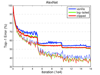
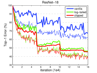
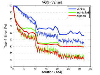
Substantial gains were obtained by training the activation quantized networks from scratch. Although the vanilla ReLU had reasonable performance as backwards approximator for AlexNet, much better results were achieved with the clipped ReLU of (12) and the log-tailed ReLU of (13). Figure 5 shows that the larger gradient mismatch of the vanilla ReLU created instabilities in the optimization, for all networks. However, these instabilities were more serious for the deeper networks, such as ResNet-18 and VGG-Variant. This explains the sharper drop in performance of the vanilla ReLU for these networks, in Table 3. Note, in Figure 5, that the clipped ReLU and the log-tailed ReLU enabled more stable learning and reached a much better optimum for all networks. Among them, the log-tailed ReLU performed slightly better than the clipped ReLU on AlexNet, but slightly worse on ResNet-18 and VGG-Variant. To be consistent, “clipped ReLU” was used in the following sections.
| quantization type | non-uniform | uniform | none | |||||
|---|---|---|---|---|---|---|---|---|
| levels | 2 | 3 | 7 | 15 | 3∗ | 7∗ | BW | |
| AlexNet | Top-1 | 48.6 | 50.6 | 52.4 | 52.6 | 50.5 | 51.9 | 52.4 |
| Top-5 | 72.8 | 74.3 | 75.8 | 76.2 | 74.6 | 75.7 | 75.9 | |
| ResNet-18 | Top-1 | 54.5 | 57.6 | 60.3 | 60.8 | 56.1 | 59.6 | 61.3 |
| Top-5 | 78.5 | 81.0 | 82.8 | 83.4 | 79.7 | 82.4 | 83.6 | |
5.5 Bit-width Impact
The next set of experiments studied the bit-width impact of the activation quantization. In all cases, weights were binarized. Table 4 summarizes the performance of AlexNet and ResNet-18 as a function of the number of quantization levels. While the former improved with the latter, there was a saturation effect. The default HWGQ configuration, also used in all previous experiments, consisted of two non-uniform positive quantization levels plus a “0”. This is denoted as “2” in the table. For AlexNet, this very low-bit quantization sufficed to achieve recognition rates close to those of the full-precision activations. For this network, quantization with seven non-uniform levels was sufficient to reproduce the performance of full-precision activations. For ResNet-18, however, there was a more noticeable gap between low-bit and full-precision activations. For example, “3” outperformed “2” by 3.1 points for ResNet-18, but only 2.1 points for AlexNet. These results suggest that increasing the number of quantization levels is more beneficial for ResNet-18 than for AlexNet.
So far we have used non-uniform quantization. As discussed in Section 4.2, this requires more bits than uniform quantization during arithmetic computation. Table 4 also shows the results obtained with uniform quantization, with superscript “”. Interestingly, for the same number of quantization levels, the performance of the uniform quantizer was only slightly worse than that of its non-uniform counterpart. But for the same bit width, the uniform quantizer was noticeably superior than the non-uniform quantizer, by comparing “2” and “3∗” (both of them need 2-bit representation during arithmetic computation).
| Model | Reference | Full | HWGQ | |
|---|---|---|---|---|
| AlexNet | Top-1 | 57.1 | 58.5 | 52.7 |
| Top-5 | 80.2 | 81.5 | 76.3 | |
| ResNet-18 | Top-1 | 69.6 | 67.3 | 59.6 |
| Top-5 | 89.2 | 87.9 | 82.2 | |
| ResNet-34 | Top-1 | 73.3 | 69.4 | 64.3 |
| Top-5 | 91.3 | 89.1 | 85.7 | |
| ResNet-50 | Top-1 | 76.0 | 71.5 | 64.6 |
| Top-5 | 93.0 | 90.5 | 85.9 | |
| VGG-Variant | Top-1 | - | 69.8 | 64.1 |
| Top-5 | - | 89.3 | 85.6 | |
| GoogLeNet | Top-1 | 68.7 | 71.4 | 63.0 |
| Top-5 | 88.9 | 90.5 | 84.9 | |
| Model | AlexNet | ResNet-18 | |||
| XNOR | DOREFA | HWGQ | XNOR | HWGQ | |
| Top-1 | 44.2 | 47.7 | 52.7 | 51.2 | 59.6 |
| Top-5 | 69.2 | - | 76.3 | 73.2 | 82.2 |
| Top-1 gap | -12.4 | -8.2 | -5.8 | -18.1 | -7.7 |
5.6 Comparison with the state-of-the-art
Table 5111The reference performance of AlexNet and GoogLeNet is at https://github.com/BVLC/caffe, and of ResNet is at https://github.com/facebook/fb.resnet.torch. Our worse ResNet implementations are probably due to fewer training iterations and no further data augmentation. presents a comparison between the full precision and the low-precision HWGQ-Net of many popular network architectures. For completeness, we consider the GoogLeNet, ResNet-34 and ResNet-50 in this section. In all cases, the HWGQ-Net used 1-bit binary weights, a 2-bit uniform HWGQ as forward approximator, and the clipped ReLU as backwards approximator. Comparing to the previous ablation experiments, the numbers of training iterations were doubled and polynomial learning rate annealing (power of 1) was used for HWGQ-Net, where it gave a slight improvement over step-wise annealing. Table 5 shows that the HWGQ-Net approximates well all popular networks, independently of their complexity or depth. The top-1 accuracy drops from full- to low-precision are similar for all networks (59 points), suggesting that low-precision HWGQ-Net will achieve improved performance as better full-precision networks become available.
Training a network with binary weights and low-precision activations from scratch is a new and challenging problem, only addressed by a few previous works [4, 32, 40]. Table 6 compares the HWGQ-Net with the recent XNOR-Net [32] and DOREFA-Net [40], on the ImageNet classification task. The DOREFA-Net result is for a model of binary weights, 2-bit activation, full precision gradient and no pre-training. For AlexNet, the HWGQ-Net outperformed the XNOR-Net and the DOREFA-Net by a large margin. Similar improvements over the XNOR-Net were observed for the ResNet-18, where DOREFA-Net results are not available. It is worth noting that the gaps between the full-precision networks and the HWGQ-Net (-5.8 for AlexNet and -7.7 for ResNet-18) are much smaller than those of the XNOR-Net (-12.4 for AlexNet and -18.1 for ResNet-18) and the DOREFA-Net (-8.2 for AlexNet). This is strong evidence that the HWGQ is a better activation quantizer. Note that, in contrast to the experimentation with one or two networks by [4, 32, 40], the HWGQ-Net is shown to perform well for various network architectures. To the best of our knowledge, this is the first time that a single low-precision network is shown to successfully approximate many popular networks.
5.7 Results on CIFAR-10
In addition, we conducted some experiments on the CIFAR-10 dataset [21]. The network structure used, denoted VGG-Small, was similar to that of [4] but relied on a cross-entropy loss and without two fully connected layers. The learning strategy was that used in the VGG-Variant of Section 5.1, but the mini-batch size was 100 and the learning rate was divided by 10 after every 40K iterations (100K in total). The data augmentation strategy of [13] was used. As in Section 5.6, polynomial learning rate decay was used for low-precision VGG-Small. The HWGQ-Net results are compared with the state-of-the-art in Table 7. It can be seen that the HWGQ-Net achieved better performance than various popular full-precision networks, e.g. Maxout [9], NIN [27], DSN [23], FitNet [34], and than various low precision networks. The low-precision VGG-Small drops 0.67 points when compared to its full-precision counterpart. These findings are consistent with those on ImageNet.
| precision | Method | error (%) |
| Full + Full | Maxout [9] | 9.38 |
| NIN [27] | 8.81 | |
| DSN [23] | 8.22 | |
| FitNet [34] | 8.39 | |
| ResNet-110 [13] | 6.43 | |
| VGG-Small | 6.82 | |
| 1-bit + Full | BinaryConnect [3] | 8.27 |
| 2-bit + Full | Ternary Weight Network [24] | 7.44 |
| 1-bit + 1-bit | BNN [4] | 10.15 |
| 1-bit + 2-bit | VGG-Small-HWGQ | 7.49 |
6 Conclusion
In this work, we considered the problem of training high performance deep networks with low-precision. This was achieved by designing two approximators for the ReLU non-linearity. The first is a half-wave Gaussian quantizer, applicable in the feedforward network computations. The second is a piece-wise continuous function, to be used in the backpropagation step during learning. This design overcomes the learning inefficiency of the popular binary quantization procedure, which produces a similar approximation for the less effective hyperbolic tangent nonlinearity. To minimize the problem of gradient mismatch, we have studied several backwards approximation functions. It was shown that the mismatch is most affected by activation outliers. Insights from the robust estimation literature were then used to propose the clipped ReLU and log tailed ReLU approximators. The network that results from the combination of these with the HWGQ, denoted HWGQ-Net was shown to significantly outperform previous efforts at deep learning with low precision, substantially reducing the gap between the low-precision and full-precision various state-of-the-art networks. These promising experimental results suggest that the HWGQ-Net can be very useful for the deployment of state-of-the-art neural networks in real world applications.
References
- [1] Z. Cai, Q. Fan, R. S. Feris, and N. Vasconcelos. A unified multi-scale deep convolutional neural network for fast object detection. In ECCV, pages 354–370, 2016.
- [2] W. Chen, J. T. Wilson, S. Tyree, K. Q. Weinberger, and Y. Chen. Compressing neural networks with the hashing trick. In ICML, pages 2285–2294, 2015.
- [3] M. Courbariaux, Y. Bengio, and J. David. Binaryconnect: Training deep neural networks with binary weights during propagations. In NIPS, pages 3123–3131, 2015.
- [4] M. Courbariaux, I. Hubara, D. Soudry, R. El-Yaniv, and Y. Bengio. Binarized neural networks: Training neural networks with weights and activations constrained to +1 or -1. CoRR, abs/1602.02830, 2016.
- [5] M. Denil, B. Shakibi, L. Dinh, M. Ranzato, and N. de Freitas. Predicting parameters in deep learning. In NIPS, pages 2148–2156, 2013.
- [6] E. L. Denton, W. Zaremba, J. Bruna, Y. LeCun, and R. Fergus. Exploiting linear structure within convolutional networks for efficient evaluation. In NIPS, pages 1269–1277, 2014.
- [7] R. B. Girshick. Fast R-CNN. In ICCV, pages 1440–1448, 2015.
- [8] Y. Gong, L. Liu, M. Yang, and L. D. Bourdev. Compressing deep convolutional networks using vector quantization. CoRR, abs/1412.6115, 2014.
- [9] I. J. Goodfellow, D. Warde-Farley, M. Mirza, A. C. Courville, and Y. Bengio. Maxout networks. In ICML, pages 1319–1327, 2013.
- [10] S. Han, H. Mao, and W. J. Dally. Deep compression: Compressing deep neural network with pruning, trained quantization and huffman coding. CoRR, abs/1510.00149, 2015.
- [11] S. Han, J. Pool, J. Tran, and W. J. Dally. Learning both weights and connections for efficient neural network. In NIPS, pages 1135–1143, 2015.
- [12] K. He, X. Zhang, S. Ren, and J. Sun. Delving deep into rectifiers: Surpassing human-level performance on imagenet classification. In ICCV, pages 1026–1034, 2015.
- [13] K. He, X. Zhang, S. Ren, and J. Sun. Deep residual learning for image recognition. In CVPR, pages 770–778, 2016.
- [14] G. E. Hinton, N. Srivastava, A. Krizhevsky, I. Sutskever, and R. Salakhutdinov. Improving neural networks by preventing co-adaptation of feature detectors. CoRR, abs/1207.0580, 2012.
- [15] P. J. Huber et al. Robust estimation of a location parameter. The Annals of Mathematical Statistics, 35(1):73–101, 1964.
- [16] A. Hyvärinen and E. Oja. Independent component analysis: algorithms and applications. Neural Networks, 13(4-5):411–430, 2000.
- [17] F. N. Iandola, M. W. Moskewicz, K. Ashraf, S. Han, W. J. Dally, and K. Keutzer. Squeezenet: Alexnet-level accuracy with 50x fewer parameters and <1mb model size. CoRR, abs/1602.07360, 2016.
- [18] S. Ioffe and C. Szegedy. Batch normalization: Accelerating deep network training by reducing internal covariate shift. In ICML, pages 448–456, 2015.
- [19] M. Jaderberg, A. Vedaldi, and A. Zisserman. Speeding up convolutional neural networks with low rank expansions. In BMVC, 2014.
- [20] Y. Jia, E. Shelhamer, J. Donahue, S. Karayev, J. Long, R. B. Girshick, S. Guadarrama, and T. Darrell. Caffe: Convolutional architecture for fast feature embedding. In MM, pages 675–678, 2014.
- [21] A. Krizhevsky. Learning multiple layers of features from tiny images. 2009.
- [22] A. Krizhevsky, I. Sutskever, and G. E. Hinton. Imagenet classification with deep convolutional neural networks. In NIPS, pages 1106–1114, 2012.
- [23] C. Lee, S. Xie, P. W. Gallagher, Z. Zhang, and Z. Tu. Deeply-supervised nets. In AISTATS, 2015.
- [24] F. Li and B. Liu. Ternary weight networks. CoRR, abs/1605.04711, 2016.
- [25] D. D. Lin and S. S. Talathi. Overcoming challenges in fixed point training of deep convolutional networks. CoRR, abs/1607.02241, 2016.
- [26] D. D. Lin, S. S. Talathi, and V. S. Annapureddy. Fixed point quantization of deep convolutional networks. In ICML, pages 2849–2858, 2016.
- [27] M. Lin, Q. Chen, and S. Yan. Network in network. CoRR, abs/1312.4400, 2013.
- [28] Z. Lin, M. Courbariaux, R. Memisevic, and Y. Bengio. Neural networks with few multiplications. CoRR, abs/1510.03009, 2015.
- [29] S. P. Lloyd. Least squares quantization in PCM. IEEE Trans. Information Theory, 28(2):129–136, 1982.
- [30] V. Nair and G. E. Hinton. Rectified linear units improve restricted boltzmann machines. In ICML, pages 807–814, 2010.
- [31] R. Pascanu, T. Mikolov, and Y. Bengio. On the difficulty of training recurrent neural networks. In ICML, pages 1310–1318, 2013.
- [32] M. Rastegari, V. Ordonez, J. Redmon, and A. Farhadi. Xnor-net: Imagenet classification using binary convolutional neural networks. In ECCV, pages 525–542, 2016.
- [33] S. Ren, K. He, R. B. Girshick, and J. Sun. Faster R-CNN: towards real-time object detection with region proposal networks. In NIPS, pages 91–99, 2015.
- [34] A. Romero, N. Ballas, S. E. Kahou, A. Chassang, C. Gatta, and Y. Bengio. Fitnets: Hints for thin deep nets. CoRR, abs/1412.6550, 2014.
- [35] O. Russakovsky, J. Deng, H. Su, J. Krause, S. Satheesh, S. Ma, Z. Huang, A. Karpathy, A. Khosla, M. S. Bernstein, A. C. Berg, and F. Li. Imagenet large scale visual recognition challenge. International Journal of Computer Vision, 115(3):211–252, 2015.
- [36] K. Simonyan and A. Zisserman. Very deep convolutional networks for large-scale image recognition. CoRR, abs/1409.1556, 2014.
- [37] C. Szegedy, W. Liu, Y. Jia, P. Sermanet, S. E. Reed, D. Anguelov, D. Erhan, V. Vanhoucke, and A. Rabinovich. Going deeper with convolutions. In CVPR, pages 1–9, 2015.
- [38] V. Vanhoucke, A. Senior, and M. Z. Mao. Improving the speed of neural networks on cpus. In Deep Learning and Unsupervised Feature Learning Workshop, NIPS 2011, 2011.
- [39] M. D. Zeiler, M. Ranzato, R. Monga, M. Z. Mao, K. Yang, Q. V. Le, P. Nguyen, A. W. Senior, V. Vanhoucke, J. Dean, and G. E. Hinton. On rectified linear units for speech processing. In ICASSP, pages 3517–3521, 2013.
- [40] S. Zhou, Z. Ni, X. Zhou, H. Wen, Y. Wu, and Y. Zou. Dorefa-net: Training low bitwidth convolutional neural networks with low bitwidth gradients. CoRR, abs/1606.06160, 2016.