A method of limiting performance loss of CNNs in noisy environments

Abstract

Convolutional Neural Network (CNN) recognition rates drop in the presence of noise. We demonstrate a novel method of counteracting this drop in recognition rate by adjusting the biases of the neurons in the convolutional layers according to the noise conditions encountered at runtime.

We compare our technique to training one network for all possible noise levels, dehazing via preprocessing a signal with a denoising autoencoder, and training a network specifically for each noise level. Our system compares favorably in terms of robustness, computational complexity and recognition rate.

1 Background

Extracting or detecting signals in noise is a topic of long standing interest in fields such as speech recognition [6, 9] and image processing [3]. In the field of neural networks, denoising autoencoders have been developed and their use to remove noise from images has been suggested [17]. In the area of convolutional neural networks, operating in noisy environments reduces recognition rates [14]. However, training with noisy input improves the ability of the network to detect signals in the presence of noise and such noisy trained networks also perform well in the absence of noise [16, 4].

How a CNN performs in the presence of noisy inputs is becoming increasingly important due to their use in autonomous vehicles. In that case, rain, snow, and fog make it difficult to detect and identify other objects on the road. Snow also makes it difficult to determine the vehicle’s position relative to the road [7, 15].

The most obvious method is to train, perhaps smaller, networks for each possible expected level of occlusion. In our experiments, this method gives the best performance in terms of detection rate; however, it is cumbersome in realize in practice because each noise level has to have its own set of parameters. Loading and unloading all the parameters for a large network at runtime could start to take significant time and energy. Furthermore, storage space would have to be provided for each set of parameters. For multiple copies of large networks, this can easily require multi-GBs, so cost of storage memory could become an issue.

To avoid having to deal with multiple sets of network parameters, one common way of dealing with snow, rain and other forms of occlusion is to train a network with a wide range, or mix, of representative input conditions [5]. However, while this method performs well over a wide range of noise levels, it does not perform as well as other methods at the extreme edges of no noise and lots of noise.

Our method requires the parameter sets at each extreme of an expected occlusion/noise range. It receives a measurement of the amount of occlusion in the environment and uses that measurement to select which parameter set to use, the zero noise parameter set or the max noise parameter set. It loads the parameters of the required parameter set into the network, then adjusts the biases of the input convolutional layer to help counteract the effects of noise.

To the best of our knowledge, there are no other works that dynamically tune an individual part of a network at runtime to improve performance in the presence of noise. In fact, while dehazing an image seems to be an active area of research [13], there seems to be little work with CNN based vision systems and noise. This could be due to the lack of a standard noisy version of the KITTI [8] dataset or similar benchmark dataset that would make comparison across works easy.

For the works that do exist, some works fuse mutliple types of input information to improve robustness to noise, [18]. Other works, such as [12], propose more sophisticated network architectures. For the most part, previous works appear to consider the network as a monolithic whole. For example, [5] trains the whole network against a mixed dataset. Our system is not mutually exclusive to these techniques and can be used in conjunction with them.

In the following sections we describe a basic convolutional neural network, review binary hypothesis testing, describe our method in more detail and our experiments, their results, and present our conclusions.

1.1 Basic CNN Model

A simple way to think about a CNN is as a collection of matched filters (equivalently correlators) connected to a truth table, Fig.1. Each correlator performs a binary hypothesis test on each region of the input image to which it is exposed. If, according to the binary hypothesis test, there is a match between the object encoded in the filter and the area of the image the filter is looking at, a ‘1’ is output otherwise a ‘0’ is output. If a certain subset of the filters find their target shape, then a particular line in a truth table is looked up. If there is an object that corresponds to that line, then the output corresponding to that object goes high. Any object that is not associated with some combination of the objects in the matched filters cannot be detected.

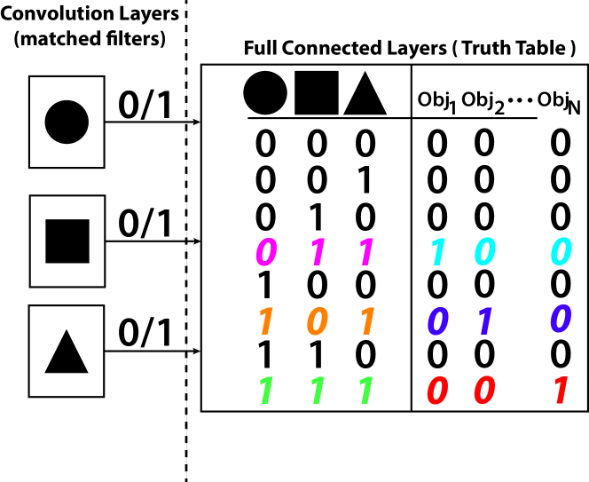
Figure 1: A CNN can be thought of as a collection of matched filters attached to a truth table. In this example, presenting an image to the CNN projects that image onto the circle, square, triangle basis.

1.2 Binary Hypothesis Test

Eq.1 shows the two hypotheses for our system. Here, $H_{0}$ is the hypothesis that the observed data, $\mathbf{y}$, is just random noise, $\mathbf{w}$. $H_{1}$ is the hypothesis that there is some deterministic signal of interest, ‘$S$’ in the observation $\mathbf{y}$.

$$\begin{split}H_{0}&:\mathbf{y}=\ \ \ \ \ \ \ \mathbf{w}\\ H_{1}&:\mathbf{y}=S+\mathbf{w}\end{split}$$ (1)

The minimum probability of error decision rule corresponds to the picking the hypothesis with the maximum a posteriori probability (MAP), Eq.2,

$$\hat{H}(\mathbf{y})=\underset{A\in\{H_{0},H_{1}\}}{\text{arg max}}Pr[H=A|\mathbf{y}=y]$$ (2)

where $y$ is a realization of $\mathbf{y}$.

For additive white Gaussian noise (AWGN), Eq.3,

$$\mathbf{w}\sim N(m_{\mathbf{w}},\sigma^{2}_{\mathbf{w}}I)$$ (3)

the MAP decision rule, Eq.2 becomes Eq.4

$$<S,\mathbf{y}>\overset{\hat{H}(\mathbf{y})=H_{1}}{\underset{\hat{H}(\mathbf{y})=H_{0}}{\gtreqless}}\frac{<S,S>}{2}+<S,m_{\mathbf{w}}>+\sigma^{2}_{\mathbf{w}}\ln(\frac{P_{0}}{P_{1}})$$ (4)

Here $<a,b>$ is shorthand for the inner product of $a$ with $b$ using the definition of inner product for whatever Hilbert space on which $a$ and $b$ are defined. Letting $\gamma$ be the right hand side of Eq. 4, as in Eq.5, and moving it to the left hand side of the inequality, gives Eq. 6.

$$\gamma\equiv\frac{<S,S>}{2}+<S,m_{\mathbf{w}}>+\sigma^{2}_{\mathbf{w}}\ln(\frac{P_{0}}{P_{1}})$$ (5)

$$\begin{split}<S,\mathbf{y}>-\gamma(S,\mathbf{w},P_{0},P_{1})&\overset{\hat{H}(\mathbf{y})=H_{1}}{\underset{\hat{H}(\mathbf{y})=H_{0}}{\gtreqless}}0\end{split}$$ (6)

Eq.6 shows that a binary hypothesis test’s threshold $\gamma$ is dependent on the noise, $\mathbf{w}$.

1.3 Binary Classification via a Single Neuron

A single neuron with a Heavyside activation function, Fig.2, implements a binary classifier Eq.7.

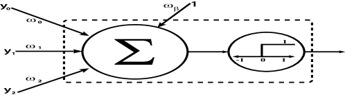
Figure 2: A neuron consists of weighted inputs, a means of combination and an output non-linearity called an activation function.

$$<\boldsymbol{\omega},\mathbf{y}>+\omega_{\beta}\overset{\hat{H}(\mathbf{y})=1}{\underset{\hat{H}(\mathbf{y})=0}{\gtreqless}}0$$ (7)

By pattern matching between Eq.6 and Eq.7, the weights $\boldsymbol{\omega}$ encode the signal of interest ‘$S$’ and the bias term, $\omega_{\beta}$, corresponds to the threshold $\gamma$. Therefore, a neuron is a machine which implements the MAP decision rule in the presence of additive Gaussian noise. Since $\gamma$, Eq.6, is a function of the noise, $\mathbf{w}$, in order to maintain performance when the noise conditions change, the neuron’s bias must also change.

1.4 Deviations from the model

There are two major deviations from the theory. First, the signal being looked for, $S$, encoded into the weights of a match filter also changes with a change in the noise level. Second, the activation function isn’t a Heaviyside step function, and therefore, a neural network isn’t purely a binary machine.

The $S$ encoded into the neuron’s weights vary with noise. This follows from the fact that object features that are visible and can be used for training when there is no noise, may be occluded when training with noise. Therefore, the $S$s when training with noise and without noise are not necessarily going to be the same. Since features that are visible in the presence of noise will also be visible when there is no noise, one can expect, and it has been observed, both here an in [16], that a network trained on noisy inputs will stand up better to a lessening of noise level than a clean trained network will to an increase in noise level.

Next, the weights, $\boldsymbol{\omega}$ are estimated from input data used for training, $\mathbf{y}_{train}$. This means that the $S$ encoded by the weights is not a known deterministic function, as had been assumed in Sec.1.2. Instead, the $S$ encoded in the neuron’s weights is really $\hat{S}(\mathbf{y}_{train})$, an estimate of the true $S$, so it is a function of the input signal used during training $\mathbf{y}_{train}$ and thus a function of the noise.

Also, in order to have continuous derivatives when doing back propogation during training, the activation function is typically a smooth differentiable function like a sigmoid or tanh, not a discontinous Heavyside step function. In this paper, we use tanh. This means that more information besides just present or not present is being transmitted from the first convolutional layer to the next. In this case, one might expect, and we show, that adjusting the biases of the layers besides the input convolutional layer might have an impact of performance. It would also be expected that the inner layer’s impact would decrease as the chosen activation function becomes closer to the Heavyside function. Demonstrating this is for future work.

2 Proposed Method - Adjusting Biases

Following directly from the theory in Sec.1.2, our method is to simply adjust the biases of the input convolutional layer or layers in occordinance with the noise in the input signal. This method changes the threshold to the correct threshold for detection at that level of noise. Comparing the output of our correlator to the correct threshold dramatically improves the ability of the network to handle changes in input noise. This kind of situation could occur in numerous applications like automotive applications or simple street sign/address recognintion during rain or fog. The noise could be random occlusion caused by rain or snow or background noise caused by bright sun or darkness.

Data about the amount of rain or snow falling in the area could be acquired by direct measurement by onboard sensors and/or by information received by the vehicle via some network. If a measured noise level falls between two noise levels that were used for training, interpolation can be used to create appropriate biases for the measured noise level. If a measured noise level falls outside the expected range, interpolation can once again be used, if it is safe to do so. Our method comprises both a training stage, Sec.2.1, and a runtime operation stage, Sec.2.1.1.

2.1 Training

Fig.3 shows the training flow. In order to train for noise, we need to select an appropriate range of expected noise levels. The minimum expected noise level will be referred to as the zero or clean noise level. In our tests, this is the absence of any noise. The maximum expected noise level will be called the max or dirty noise level. All network parameters are trained for each of these two different noise levels. Then, the clean parameters are loaded into the network and the network is trained for each individual noise level. This time, only the biases on the input convolution layer (or layers) are allowed to train and are saved for each individual noise level. This is repeated for the max noise set. Each set of params, the zero set and the max set will now have an associated set of biases for each noise level.

2.1.1 Runtime Operation

The runtime flow is shown in Fig.4. During runtime, the ambient noise level is being continuously measured. This is then used to first select the appropriate parameter set zero or max. Then it is again used to select which set of biases should be used for that noise level. If the measured noise does not exactly match a bias, the nearest bias set can be used, or interpolation can be used to quickly create a better fitting bias set.

Noise isn’t always just zero mean AWGN. Sometimes it is non-zero mean noise. Noise like this is more like camouflage. The ambient lighting may make the background much lighter or darker. Thus making it more difficult to distinguish the object from the background. This creates three situations for our matched filters,

$$\begin{split}<S,\mathbf{k}>&\mathbf{=}<S,S>\\ <S,\mathbf{k}>&\mathbf{<}<S,S>\\ <S,\mathbf{k}>&\mathbf{>}<S,S>\\ \end{split}$$ (8)

Where $\mathbf{k}$ is the background of the image. When the background and $S$ are similar in color and intensity, $<S,\mathbf{k}>=<S,S>$. This makes detection very difficult. When $<S,\mathbf{k}><<S,S>$, the normal decision rule of Eq.6 applies. However, when $<S,\mathbf{k}>><S,S>$, the hypothesis need to be reversed as in Eq.9.

$$\begin{split}<S,\mathbf{y}>-\gamma(S,\mathbf{w},P_{0},P_{1})&\overset{\hat{H}(\mathbf{y})=H_{0}}{\underset{\hat{H}(\mathbf{y})=H_{1}}{\gtreqless}}0\end{split}$$ (9)

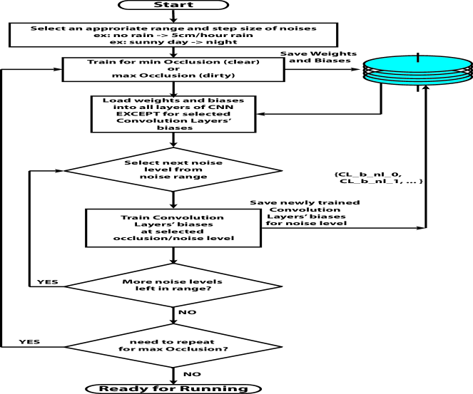
Figure 3: A flow diagram of our training methodology.

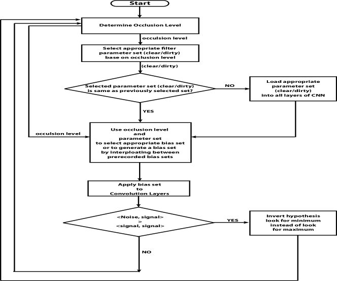
Figure 4: A flow diagram of our running methodology.

3 Test Setup

We used the LeNet model[10] for Theano [2] that is avilable on the lisa-lab DeepLearningTutorials [1] from gitHub. This model is made up of two convolutional layers, one hidden layer and a logistic regression layer. The layers have 20 filters, 50 filters, 500 neurons and 10 neurons respectively.

Each image in the MNIST dataset[11] is 28x28 pixels whose intensity is in the range $[0,1]$. Each image was corrupted with AWGN of a particular standard deviation. Multiple datasets were created, one set for each noise with a specific standard deviation in the range of $[0,1]$. Modified pixels whose values exceeded either extreme were clamped to that exterme value. Fig.5 shows a representative set of images of the number 2 with increasing amounts of AGWN.

We test four different kinds of networks: network trained at each noise level, a mixed noise trained network, a zero noise trained network, and a max noise trained network. All networks were trained on a batch size 1000 with a learning rate of 0.05 and 1000 epochs maximum.

Noise is not just restricted to zero mean Gaussian noise. Noise can also come in the form of a scene being too bright or too dark. Therefore, we also tested our system with MNIST numbers that have a background that varies in intensity as seen in Fig.6. These changing background level results are seen in Sec.4.5.

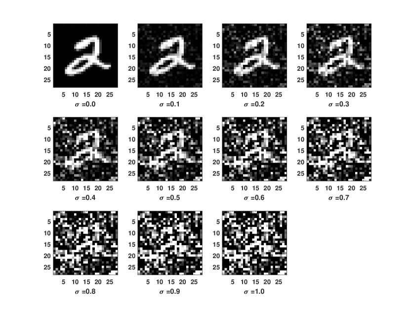
Figure 5: The MNIST number 2 is corrupted with zero mean AWGN.

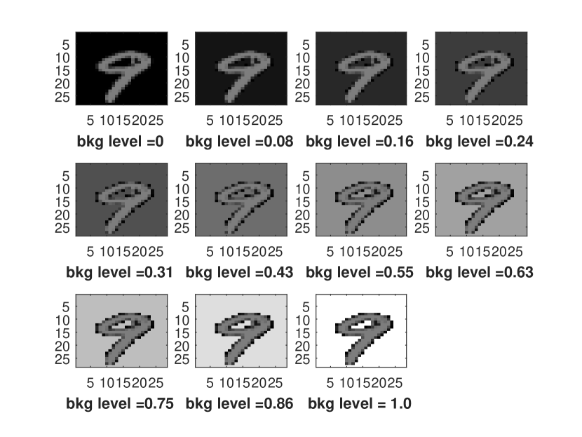
Figure 6: The MNIST number 9 is corrupted with a uniform background noise of different intensities.

Finally, we run tests were we preprocessed the noisy input images with a denoising autoencoder (dA). Like the LeNet CNN, the dA used was taken from the Theano tutorials. It was a single hidden layer autoencoder with 500 hidden nodes. The dA was used as a preprocessor to the aforementioned LeNet network. The dA, takes in a corrupted image, and outputs a cleaned up version of that image. The cleaned up image was then input into the LeNet network. The LeNet network was trained using an unaltered MNIST database. The dA used at each noise level was either a dA that had been trained for the zero or max noise levels or for a mix of noise levels.

4 Results

This section presents results for all comparisons. In all situations, training for and testing on a specific noise level lead to the best results. This method, however, may be too heavy on system resouces and does not allow for the ability to modify the system when the measured noise does not exactly match a trained noise level. Pruning may be used, however, this can lead to more sensitivity to noise as was observed in [16].

4.1 Impact of zero mean finite variance AWGN

Fig.7 is a plot of standard deviation of AWGN vs detection rate for the base methods: all parameters trained (and therefore adjusted) at all noise levels, all parameters were trained with a mixed noise dataset, a zero noise trained network and a max noise trained network. The highest performing network at each noise level is the network has been trained for that specific noise level. This is denoted by the line with the square markers. The circle line is for the network that was trained with a mix of data that was drawn from the entire noise range. The hexagram line uses the parameters from the maximum noise level trained network. The star line uses the parameters for the zero noise level trained network.

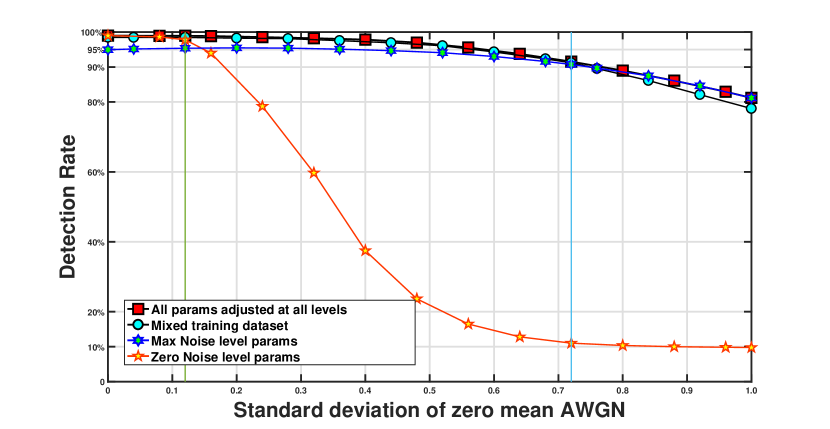
Figure 7: The mixed trained network outperforms the zero noise and max noise networks in the range [0.12,0.72].

As can be seen, training for each noise level maximizes performance at that noise level, but this takes considerable storage space and swapping out parameters on such a fine scale may be taxing on system resources.

Training with the mixed noise level dataset creates the best performing network over the widest range possible when using only a single set of parameters. Since storage and memory bandwidth are at a premium in a real time system, this is the most practical alternative to our system. However, mixed noise training is not a performance leader at either end of the noise spectrum. Using it would only be optimal if there was a perpetual level of occlusion.

As seen in Fig.7, the zero noise trained network out performs the mixed noise trained network until a standard deviation of about 0.12. This is marked by a veritcal line. The max noise network outperforms the mixed noise network in the standard deviation noise range of [0.72,1.0]. This leaves a wide range, [0.12, 0.72] in which the mixed noise trained network is the simplest and most robust network. The 0.72 standard deviation is also accented by a vertical line.

As expected, the maximum noise trained network holds up to a change in its noise environment better than the zero noise trained network. As stated earlier, this kind of behavior has been observed before [16]. This is reasonable because the features learned when training with noise, if the noise is white noise, should be there whether the noise is present or not. However, the features learned when training without noise, may become corrupted or totally obstructed in an image with noise.

4.2 Adjusting input convolution layer biases

Fig.8 shows the impact of adjusting the input convolution layer’s biases when using the zero noise parameter set. Adjusting the biases extends the range on which the zero noise network outperforms the mixed network from 0.12 to around 0.36. Furthermore, the worst the zero noise network now performs improves from around 10% to around 60%, approximately a 6x improvement in performance.

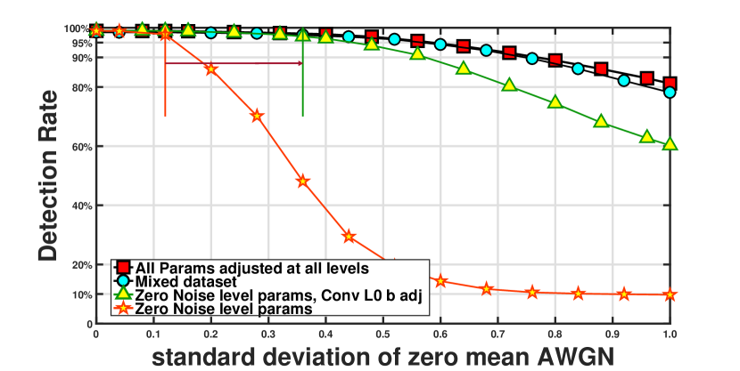
Figure 8: Adjusting the biases of the input convolution layer extends the upper noise limit of the region where the zero noise level parameters out perform the mixed noise level parameters from 0.12 to 0.36. Here the zero noise parameters were used for testing.

4.3 Adjusting multiple convolution layers biases

Fig.9 shows that adjusting both of the convolution layer’s biases leads to further improvements in detection performance. This behavior is not expected when using Heavyside activation functions. However, the activation function is $tanh(x)$, so more information than just a binary result is being transmitted to the next layer. This improvement is also understandable in that adjusting the biases of the inner layers makes the network closer to the best performing network that had been trained just for that layer.

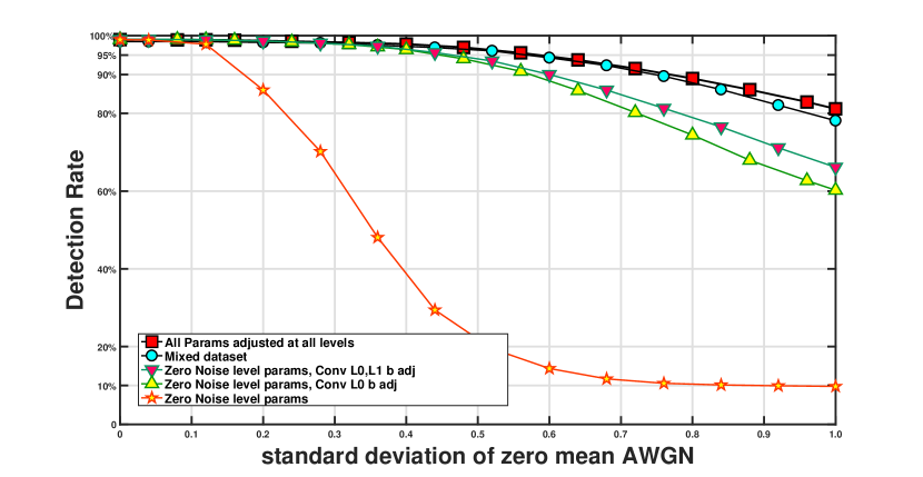
Figure 9: Adjusting the biases of both convolution layers results in better performance.

4.4 Adjusting Max noise network

Fig.10 shows how the max noise network’s performance improves with bias adjustment. The region in which it beats the mixed noise network goes from 0.72 to about 0.68, not as big of an improvement as observed with the zero noise network.

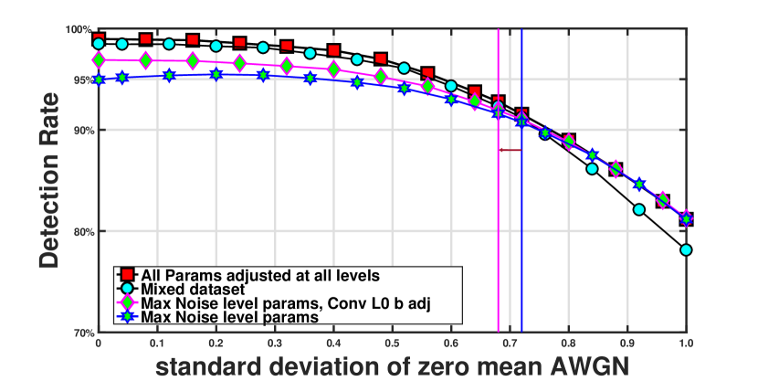
Figure 10: Effect of adjusting noisy filters’ biases.

Fig.11 recreates Fig.7, but with the zero noise network and max noise network’s biases adjusted. This shrinks the area in which the mixed training is better than adjusting biases from [0.12,0.72] to [0.36, 0.68].

This results in a range of operation between 0.36 and 0.68 in which the mixed noise network out performs the other two bias adjusted networks.

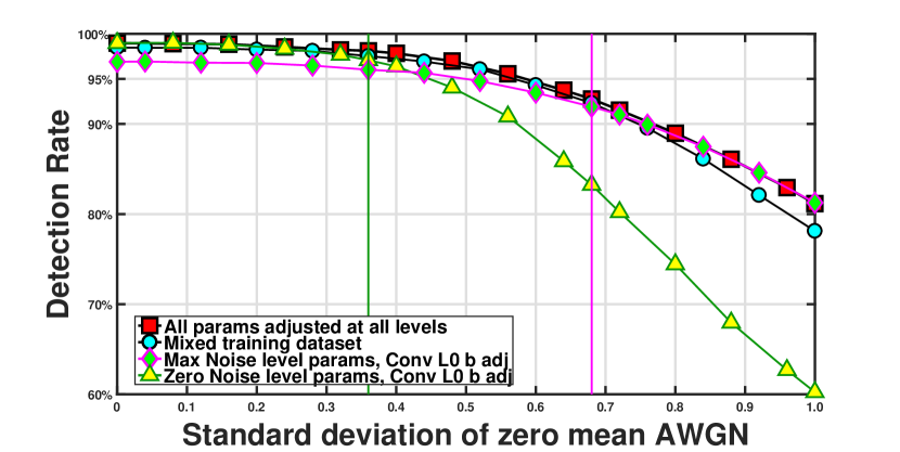
Figure 11: Adjusting the biases of the zero and max noise networks significantly decreases the mixed noise trained network’s optimal range from the range seen in Fig.7.

4.5 Changing background level

There are two situations to consider when changing the background level. The first is that the noise is at the same level as the interior. The first case results in Fig.12. Here, rule reversal doesn’t matter as the network has been trained on a mean noise level of 0.5 and the body of each letter is also 0.5. This means that, in order for detection to work, the network does not use the character’s body information. It only learns about the small perturbations at the edge of the letter. Some of these perturbations can be seen around the letters in Fig.6. By inspection, it seems that these edge markers were somewhat more likely to be dark than light, so this explains the drop in performance as the background becomes more dark. Dark is indicated by a noise level of 0.0 and a clear background is a noise level of 1.0.

The second situation is when the network has been trained with one of the two extremes of noise. The second situation results in Fig.13. In this case, if rule reversal is not utilized, the performance of the networks drops dramatically when approaching and after crossing the half way mark in the direction away from the trained noise level. If rule reversal is used, then performance drops as the ambient level approached the 0.5 mark and then returns back up as the ambient level again diverges from the level of the inner part of a character.

This suggests that training under ambient lighting conditions that are about the same level as the object you are trying detect is the best policy for minimizing the effects of changes in ambient lighting conditions. This is to say that, one should try to camouflage the object they are trying to detect when training. This again goes back to the idea that features that are learnable in the presence of camouflage are going to be there even when the camouflage is removed.

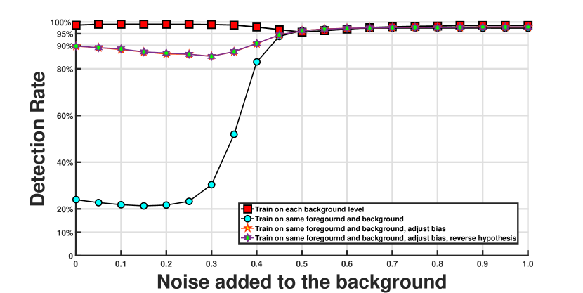
Figure 12: Bias adjustment helps maintain detection rate. Noise level is the mean noise value and not the variance.

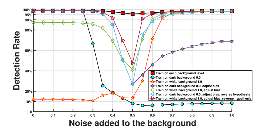
Figure 13: The network has been trained at extremes of background levels. Both rule reversal and bias adjustment should be used in order to maintain performance.

4.6 Denoising AutoEncoder as preprocessor

Denoising autoencoders can be used to remove noise from images. However, dAs are very computationally intensive, so they may not be well suited for an embedded environment. If the case of the dA, once again, training without noise leads to the worst performance. Training with noise gives performance slightly better than our bias technique for the max noise level in the low noise regime. However, it does not match the performance of our technique for the zero noise trained bias controlled network, Fig.14.

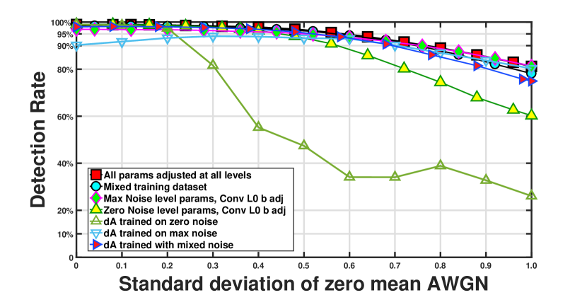
Figure 14: Denoising autoencoder performs well over a large range when trained with a mixed dataset; however, it doesn’t perform as well as our methoid in the extreme regions or the network itself just trained with mixed data.

5 Conclusions and Future Work

Networks trained for individual noise levels seem to have the best performance. Mixed noise trained networks perform well on average, but not at the extremes, so such a network would be suboptimal when conditions are good and possibly dangerously subobitmal when it is needed the most in bad conditions. The noisy bias adjusted network performs well when there is lots of noise, but the the clean trained bias adjusted network peforms better when there is low levels of noise. In short, there seems to be no optimal network for all noise levels.

Also, because of their computational complexity, preprocessing a signal with a denoising autoencoder does not look to be as effective as one might initially hope.

Our technique of adjusting the biases of the convolutional layers helps support detection performance in the presence of a change in noise level from that with which the network was trained. It has been shown to extend the effective range for both the zero noise parameters and the max noise parameters. Adjusting the biases is computationally efficient and simple to implement and is this an attractive part of a possible solution. How this technique can be used in a specific situation will require further research.

References

- [1] Deep learning tutorials. https://github.com/lisa-lab/DeepLearningTutorials, Nov. 2016.
- [2] R. Al-Rfou, G. Alain, A. Almahairi, et al. Theano: A Python framework for fast computation of mathematical expressions. arXiv e-prints, abs/1605.02688, May 2016.
- [3] J. Besag. On the statistical analysis of dirty pictures. JOURNAL OF THE ROYAL STATISTICAL SOCIETY B, 48(3):48–259, 1986.
- [4] C. M. Bishop. Training with noise is equivalent to tikhonov regularization. Neural Comput., 7(1):108–116, Jan. 1995.
- [5] M. Bojarski, D. D. Testa, D. Dworakowski, et al. End to end learning for self-driving cars. CoRR, abs/1604.07316, 2016.
- [6] C. Cerisara, L. Rigazio, and J.-C. Junqua. -jacobian environmental adaptation. Speech Communication, 42(1):25 – 41, 2004. Adaptation Methods for Speech Recognition.
- [7] A. Davies. The clever way ford’s self-driving cars navigate in snow. https://www.wired.com/2016/01/the-clever-way-fords-self-driving-cars-navigate-in-snow/, Jan. 2016.
- [8] A. Geiger, P. Lenz, C. Stiller, and R. Urtasun. Vision meets robotics: The kitti dataset. International Journal of Robotics Research (IJRR), 2013.
- [9] Y. Gong. Speech recognition in noisy environments: A survey. Speech Commun., 16(3):261–291, Apr. 1995.
- [10] Y. Lecun, L. Bottou, Y. Bengio, and P. Haffner. Gradient-based learning applied to document recognition. Proceedings of the IEEE, 86(11):2278–2324, Nov 1998.
- [11] Y. Lecun and C. Cortes. The MNIST database of handwritten digits.
- [12] B.-Y. Lin and C. S. Chen. Two parallel deep convolutional neural networks for pedestrian detection. In 2015 International Conference on Image and Vision Computing New Zealand (IVCNZ), pages 1–6, Nov 2015.
- [13] S. Liu, M. A. Rahman, C. Y. Wong, et al. Image de-hazing based on optimal compression and histogram specification. In 2015 8th International Congress on Image and Signal Processing (CISP), pages 281–286, Oct 2015.
- [14] N. Pinto, D. D. Cox, and J. J. DiCarlo. Why is real-world visual object recognition hard? PLoS Computational Biology, 4(1):e27, jan 2008. PMID: 18225950.
- [15] D. Ryan. Lincoln laboratory demonstrates highly accurate vehicle localization under adverse weather conditions. http://www.ll.mit.edu/news/Highly-accurate-vehicle-localization-under-adverse-weather.html, June 2016.
- [16] J. Sietsma and R. J. F. Dow. Creating artificial neural networks that generalize. Neural Netw., 4(1):67–79, Jan. 1991.
- [17] P. Vincent, H. Larochelle, I. Lajoie, Y. Bengio, and P.-A. Manzagol. Stacked denoising autoencoders: Learning useful representations in a deep network with a local denoising criterion. J. Mach. Learn. Res., 11:3371–3408, Dec. 2010.
- [18] P. Viola, M. J. Jones, and D. Snow. Detecting pedestrians using patterns of motion and appearance. In Proceedings Ninth IEEE International Conference on Computer Vision, pages 734–741 vol.2, Oct 2003.