Attenuated Coupled Cluster: A Heuristic Polynomial Similarity Transformation Incorporating Spin Symmetry Projection Into Traditional Coupled Cluster Theory

Abstract

In electronic structure theory, restricted single-reference coupled cluster (CC) captures weak correlation but fails catastrophically under strong correlation. Spin-projected unrestricted Hartree-Fock (SUHF), on the other hand, misses weak correlation but captures a large portion of strong correlation. The theoretical description of many important processes, e.g. molecular dissociation, requires a method capable of accurately capturing both weak- and strong correlation simultaneously, and would likely benefit from a combined CC-SUHF approach. Based on what we have recently learned about SUHF written as particle-hole excitations out of a symmetry-adapted reference determinant, we here propose a heuristic coupled cluster doubles model to attenuate the dominant spin collective channel of the quadratic terms in the coupled cluster equations. Proof of principle results presented here are encouraging and point to several paths forward for improving the method further.

1 Introduction

We are interested in the simultaneous description of weak and strong correlation in electronic structure theory. Weak, or dynamical, correlation is ubiquitous and is often conceptualized as electrons instantaneously avoiding one another. The Hartree-Fock mean-field description of a weakly-correlated system is generally qualitatively correct, and a quantitative description can be provided by the coupled cluster family of methods.[1, 2, 3, 4] Strong, or static, correlation, on the other hand, is not as universally prevalent. It typically arises from degeneracies in the system, and is associated with the qualitative failure of the symmetry-adapted mean-field description. This failure, in turn, usually implies the breakdown of coupled cluster theory.

Strong correlation is often accompanied by the spontaneous breaking of a symmetry of the Hamiltonian in the mean-field reference, e.g. the breaking of $S^{2}$ in the Hartree-Fock wavefunction past the Coulson-Fischer point in a molecular dissociation curve. If one allows such symmetry breaking, e.g. unrestricted Hartree-Fock (UHF), then broken-symmetry Hartree-Fock and coupled cluster may give reasonable energies, but wrong wavefunctions, at least for finite systems where symmetry breaking is artifactual, i.e. the result of approximations.

Projected Hartree-Fock (PHF)[5, 6, 7, 8, 9, 10] describes strong correlation by restoring the symmetry-preserving component of the broken-symmetry mean-field reference. The PHF wavefunction is multideterminantal, but is compactly expressed as a linear combination of nonorthogonal determinants. When expressed using orthogonal determinants, the PHF wavefunction contains excitations to all orders, enabling the PHF wavefunction to capture strong correlation. However, PHF generally misses a large amount of the weak correlation.

Since CC captures weak correlation but fails for strong correlation, while PHF captures strong correlation but misses weak correlation, a natural question is how to combine the two methods. One option is to perform CC atop a PHF wavefunction, and work along these lines is presented elsewhere.[11][12] We here explore an alternative idea. While PHF can refer to the projection of any symmetry of the Hamiltonian broken in the mean-field reference, here, we are primarily concerned with the projection of $S^{2}$ out of an unrestricted Hartree-Fock determinant (SUHF). Although SUHF is traditionally written variationally, we have recently formulated SUHF for singlet states ($s=0$) as a polynomial similarity transformation (PoST) of particle-hole excitations out of a symmetry-adapted reference determinant in the mathematical language of traditional coupled cluster.[13, 11] In this work, we present attenuated coupled cluster (attCC), in which we use the PoST formulation of SUHF to inform a modificaton of the CCD amplitude equations that protects the method from breakdown in the presence of strong correlation.

Modifying the coupled cluster equations and $T_{2}$ operator in order to describe strong correlation has a rich history, resulting in improved descriptions of ground states, excited states and properties.[14, 15, 16, 17, 18, 19, 20, 21, 22, 23, 24, 25, 26, 27, 28] In previous work along these lines, we found that separating the singlet- and triplet pairing channels of $T_{2}$ and isolating them from one another, giving singlet-paired (CC0) and triplet-paired coupled cluster (CC1), protected CC from blowup.[27, 29] There, we decomposed $T_{2}$ along particle-particle/hole-hole (pp-hh), or ladder, channels,[30] eliminating the interaction of the channels completely. This result lead us to ask two questions: 1) can we protect coupled cluster from breakdown by attenuating, rather than severing, the dialogue between offending pairing channels? and 2) can we do so along particle-hole/particle-hole (ph-ph), or ring, channels?[31] The present work is an attempt to answer these two questions.

In what follows, we first describe traditional coupled cluster theory and SUHF in both its standard variational and our recently introduced PoST formulations. We then introduce attenuated coupled cluster and present results on some small molecules and the Hubbard Hamiltonian. Lastly, we remark on the combination of CCD with particle-number projection in the attractive pairing Hamiltonian before offering a concluding discussion.

2 Theory and Methods

2.1 Closed-Shell Coupled Cluster Theory

To avoid complicating the presentation that follows, we do not include singles in our algebraic formulation. However, the inclusion of singles is straightforward. In closed-shell coupled cluster with double excitations (CCD), we write the wave function as

$$\ket{\mathrm{CCD}}=e^{T_{2}}\ket{0},$$ (1)

where $\ket{0}$ is the restricted Hartree-Fock (RHF) reference, and the polynomial $e^{T_{2}}$ is given by

$$e^{T_{2}}=1+T_{2}+\frac{1}{2}T_{2}^{2}+\frac{1}{6}T_{2}^{3}+...$$ (2)

The cluster operator $T_{2}$ is spin adapted[32] and creates double excitations:

$$T_{2}=\frac{1}{2}t_{ij}^{ab}E_{a}^{i}E_{b}^{j},$$ (3)

where $t_{ij}^{ab}$ refers to $t_{i_{\uparrow}j_{\downarrow}}^{a_{\uparrow}b_{\downarrow}}$ in a spin-orbital formulation[33, 32], and where

$$E_{p}^{q}=p^{\dagger}_{\uparrow}q_{\uparrow}+p^{\dagger}_{\downarrow}q_{\downarrow}.$$ (4)

Here, orbitals i j (a b) are occupied (unoccupied) in the RHF reference, and summation over repeated indices is implied. We then construct a non-Hermitian, similarity-transformed Hamiltonian

$$\overline{H}=e^{-T_{2}}He^{T_{2}},$$ (5)

and obtain $T_{2}$ such that $\ket{0}$ is the right-hand eigenvector of $\overline{H}$ in the space spanned by $\ket{0}$ and the excitation manifold. Since $\overline{H}$ is non-Hermitian, $\bra{0}$ is not its left-hand eigenvector, but we can expand the left-hand eigenvector $\bra{L}$ in the space spanned by $\bra{0}$ and the excitation manifold as

$$\bra{L}=\bra{0}(1+Z_{2}),$$ (6a)

$$Z_{2}=\frac{1}{2}z_{ab}^{ij}E_{i}^{a}E_{j}^{b}.$$ (6b)

The coupled cluster energy is the biorthogonal expectiation value of $\overline{H}$, and the amplitude equations needed to make $\ket{0}$ its right-hand eigenvector and $\bra{0}(1+Z)$ its left-hand eigenvector are obtained by making the energy stationary:

$$E =\braket{0}{(1+Z_{2})\overline{H}}{0},$$ (7a)

$$0 =\frac{\partial E}{\partial t_{ij}^{ab}}=\frac{\partial E}{\partial z_{ab}^{ij}}.$$ (7b)

At convergence, the $z_{ab}^{ij}$ amplitudes do not contribute to the energy, and Eqs. 7 reduce to the familiar CCD energy and amplitude equations

$$\braket{0}{\overline{H}}{0} =E,$$ (8a)

$$\braket{{}_{ij}^{ab}}{\overline{H}}{0} =0,$$ (8b)

where $\ket{{}_{ij}^{ab}}$ is notation for referring to the space of doubly-excited determinants.[32]

With the addition of single excitations, CCSD accurately describes weakly-correlated systems. However, truncated coupled cluster methods on restricted Hartree-Fock references are known to break down when systems take on multireference character, rendering the mean field qualitatively incorrect. This breakdown is evidenced by the familiar unphysical hump in the dissociation of N₂ in the STO-3G basis, shown in Fig. 1. Although CCSD is accurate near equilibrium, the method severely overcorrelates at stretched bond lengths. For comparison, we also include results from singlet-paired CCSD (CCSD0) in Fig. 1. CCSD0 takes only the singlet-pairing channel of $T_{2}$ in Eq. 3, the effect of which is to take the symmetric piece of the doubles amplitudes[34]

$$\sigma_{ij}^{ab}=\frac{1}{2}(t_{ij}^{ab}+t_{ij}^{ba}).$$ (9)

This modification of $T_{2}$ protects the method from catastrophic failure at stretched bond lengths.

In this work, we attempt to repair CC by breaking away from the exponential ansatz. However, we would like to stress that it is not the exponential ansatz that is inherently problematic, but its combination with solving the CC equations projectively. Variational coupled cluster, in other words, does not break down due to strong correlation, though it may undercorrelate severely. While variational coupled cluster[35, 36, 37, 38, 39] is a fruitful avenue of research, it is not a panacea, and introduces additional computational complexity. We retain the standard practice of solving the CC equations projectively, and thus focus our attentions on the form of the wavefunction ansatz.

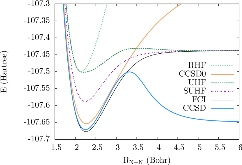
Figure 1: N₂ dissociation in STO-3G. CCSD is accurate near equilibrium, but overcorrelates at dissociation. SUHF captures strong correlation at dissociation, but misses weak correlation near equilibrium. UHF and SUHF dissociate to the correct limit due to the minimal basis. CCSD0 is protected from breakdown, but sacrifices weak correlation throughout the curve.

2.2 Projected Hartree Fock

The SUHF wavefunction for closed shells is traditionally written as a singlet ($s=0$) spin projection operator $P$ acting on the $S^{2}$-broken UHF reference, $\ket{\phi}$. Thus,

$$\ket{\mathrm{SUHF}}=P\ket{\phi},$$ (10)

and the energy is obtained variationally[10]

$$E=\frac{\braket{\phi}{P^{\dagger}HP}{\phi}}{\braket{\phi}{P^{\dagger}P}{\phi}}=\frac{\braket{\phi}{HP}{\phi}}{\braket{\phi}{P}{\phi}},$$ (11)

where we have used $P^{\dagger}=P=P^{2}$ and $[H,P]=0$. Additionally, we employ a variation-after-projection approach, in which we deliberately break symmetries and optimize the mean field in the presence of the projection operator.[9, 10] This procedure allows us to obtain the full SUHF dissociation curve in Fig. 1, rather than obtaining improved energies only past the Coulson-Fischer point.

While we would like to try to combine SUHF and CC, it is difficult to see how to do so in a straightforward manner because SUHF variationally solves for the energy as an expectation value, and CC solves for the energy and wavefunction projectively. Besides our own efforts, [13, 12, 11] there have also been other attempts to combine SUHF with residual correlation methods.[40, 41, 42] In this work, we take a new approach, exploiting our recent formulation of SUHF for singlet states as a polynomial similarity transformation of particle-hole excitations out of a symmetry-adapted reference determinant.[13, 11] Although some of the details of the PoST SUHF formulation are not key to this work, we need to establish that CC and SUHF can be written in a common language in order to justify modifying the CC equations based on the structure of the PoST SUHF equations. Briefly, we have shown that we can write the SUHF wavefunction as[13]

$$\ket{\mathrm{SUHF}}=e^{T_{1}}F(K_{2})\ket{0}.$$ (12)

In Eq. 12, $T_{1}$ is the spin symmetry adapted single-excitation operator of standard coupled cluster

$$T_{1} =t_{i}^{a}E_{a}^{i}.$$ (13a)

The polynomial $F(K_{2})$ is given by[13]

$$F(K_{2}) =1+K_{2}+\frac{3}{10}K_{2}^{2}+\frac{3}{70}K_{2}^{3}+...,$$ (14a)

which can be written as

$$F(K_{2})=\frac{\mathrm{sinh}(\sqrt{6K_{2}})}{\sqrt{6K_{2}}}.$$ (15)

The double excitation operator $K_{2}$ is

$$K_{2} =\frac{1}{2}k_{ij}^{ab}E_{a}^{i}E_{b}^{j},$$ (16a)

$$k_{ij}^{ab} =-\frac{1}{3}(u_{i}^{a}u_{j}^{b}+2u_{i}^{b}u_{j}^{a}),$$ (16b)

and $u_{i}^{a}$ are the adjustable parameters relating $\ket{0}$ to $\ket{\phi}$. More details can be found in Refs. [13, 11].

If we solve for the energy variationally, i.e.

$$E=\frac{\braket{0}{F(K_{2}^{\dagger})e^{T_{1}^{\dagger}}He^{T_{1}}F(K_{2})}{0}}{\braket{0}{F(K_{2}^{\dagger})e^{T_{1}^{\dagger}}e^{T_{1}}F(K_{2})}{0}},$$ (17)

$$0=\frac{\partial E}{\partial t_{i}^{a}}=\frac{\partial E}{\partial u_{i}^{a}},$$ (18)

we get the variational SUHF energy,[13] so we know that the polynomial form of the SUHF wavefunction is exact. However, we solve the system ‘projectively’, in a manner similar to traditional coupled cluster.[13]

We thus write a similarity transformed Hamiltonian as (cf. Eq. 5)

$$\overline{H}_{\mathrm{PHF}}=F^{-1}(K_{2})e^{-T_{1}}He^{T_{1}}F(K_{2}),$$ (19)

where the equations specifying the projective SUHF energy are

$$E =\braket{0}{(1+Z_{1})G(L_{2})\overline{H}_{\mathrm{PHF}}}{0},$$ (20a)

$$Z_{1} =\frac{1}{2}z_{a}^{i}E_{i}^{a},$$ (20b)

$$L_{2} =-\frac{1}{6}(v_{a}^{i}v_{b}^{j}+2v_{b}^{i}v_{a}^{j})E_{i}^{a}E_{j}^{b},$$ (20c)

where the $E_{i}^{a}$ excite when acting to the left, and the stationarity conditions on the energy become

$$0=\frac{\partial E}{\partial t_{i}^{a}}=\frac{\partial E}{\partial u_{i}^{a}}=\frac{\partial E}{\partial z_{a}^{i}}=\frac{\partial E}{\partial v_{a}^{i}}.$$ (21)

In Eq. 20, we define $G(L_{2})$ such that $\bra{0}G(L_{2})F^{-1}(K_{2})\approx\bra{0}F^{\dagger}(K_{2})$. To reproduce the SUHF variational energy, we need excitations in the bra up to the number of strongly correlated electrons.[13] Aside from needing a more complicated left-hand eigenvector for PoST SUHF to reproduce the variational SUHF energy, the basic mathematical structure of PoST SUHF described above is identical to that of coupled cluster. In the next section, we explain how we combine PoST SUHF with CC.

2.3 Attenuated Coupled Cluster

2.3.1 Similarity-Transformed Ansatz

We posit that coupled cluster theory breaks down in the presence of strong correlation in part because it is trying to mimic SUHF, which it cannot do, given the different polynomial forms of the two methods. When CC fails due to strong correlation, it overcorrelates, while PoST SUHF does not. One explanation is that CC has a higher coefficient than PoST SUHF on terms quadratic and higher in the amplitude equations, c.f. the $\frac{1}{2}$ on quadratic terms in Eq. 2 vs the $\frac{3}{10}$ on quadratic terms in Eq. 14. Larger coefficients results in more correlation, leading truncated CC to overcorrelate, partciularly in the strongly correlated regime where some of the doubles amplitudes factorize and become large.[13]

Our general goal in this work is to write a wavefunction that incorporates information from both the exponential similarity transformation of CC and the $sinh$ similarity transformation of SUHF. Our approach here is to write a new, double similarity transformation

$$\overline{H}_{\mathrm{attCC}}=F^{-1}(K_{2})e^{-S_{2}}He^{S_{2}}F(K_{2}),$$ (22)

where the cluster operators have the forms

$$S_{2}=\frac{1}{2}s_{ij}^{ab}E_{a}^{i}E_{b}^{j},$$ (23a)

$$K_{2}=\frac{1}{2}k_{ij}^{ab}E_{a}^{i}E_{b}^{j}.$$ (23b)

We would then solve for the energy and amplitudes projectively, as in coupled cluster theory:

$$\braket{{}_{ij}^{ab}}{\overline{H}_{\mathrm{attCC}}}{0} =0,$$ (24a)

$$\braket{0}{\overline{H}_{\mathrm{attCC}}}{0} =E.$$ (24b)

The idea is that $S_{2}$ captures dynamical correlation via the coupled cluster exponential and $K_{2}$ describes the spin collective mode and captures strong correlation via the SUHF $sinh$. We note that here we do not use the more complicated left-hand eigenvector needed for PoST SUHF using $G(L_{2})$, a potential shortcoming we discuss below.

Note that the total double-excitation operator is

$$T_{2}=S_{2}+K_{2},$$ (25)

in terms of which the similarity transformed Hamiltonian can be written

$$\overline{H}_{\mathrm{attCC}} =e^{-(T_{2}-K_{2})}F^{-1}(K_{2})HF(K_{2})e^{T_{2}-K_{2}}$$ (26a)

$$=H+[H,T_{2}]+\frac{1}{2}[[H,T_{2}],T_{2}]-\frac{1}{5}[[H,K_{2}],K_{2}]-\frac{2}{5}K_{2}[H,K_{2}]+...$$ (26b)

Thus, in practice, the energy of Eq. 24 uses the standard CCD expression, while the amplitude equations are supplemented by two terms:

$$\braket{{}_{ij}^{ab}}{\overline{H}_{\mathrm{attCC}}}{0}=\braket{{}_{ij}^{ab}}{\overline{H}_{\mathrm{CCD}}}{0}-\frac{1}{5}\braket{{}_{ij}^{ab}}{[[H,K_{2}],K_{2}]}{0}-\frac{2}{5}\braket{{}_{ij}^{ab}}{K_{2}[H,K_{2}]}{0}.$$ (27)

Everything up to this point is rigorous. What is approximate is how we obtain $K_{2}$ from $T_{2}$, determining the spin collective mode on the fly. We describe this procedure next.

2.3.2 Determining the Spin Collective Modes

In order to identify the $s_{ij}^{ab}$ and $k_{ij}^{ab}$ amplitudes, we look in the CCD $t_{ij}^{ab}$ amplitudes because spin projection is a collective phenomenon, yielding large amplitudes to all orders that should not be neglected in the strongly correlated regime.[28, 13] We write the CCD amplitudes as

$$t_{ij}^{ab}=k_{ij}^{ab}+s_{ij}^{ab},$$ (28)

and identify the spin collective mode of the CCD amplitudes by noting that the object $k_{ij}^{ab}-2k_{ij}^{ba}$ constructed with SUHF $k_{ij}^{ab}$ amplitudes from Eq. 16 is described by a single eigenvector, or collective mode, and factorizes exactly into single excitations, i.e.

$$k_{ij}^{ab}-2k_{ij}^{ba}=u_{i}^{a}u_{j}^{b}.$$ (29)

An analogus object, constructed with $t_{ij}^{ab}$ amplitudes from CC, rather than $k_{ij}^{ab}$ amplitudes from SUHF, does not factorize exactly. However, we can construct a matrix $U_{2}$ whose elements are

$$U_{ai,bj}=t_{ij}^{ab}-2t_{ij}^{ba}.$$ (30)

We then diagonalize $U_{2}$ along particle-hole lines

$$U_{ai,bj}=\sum\limits_{n}\lambda_{n}V_{ai,n}V_{bj,n},$$ (31)

where $\lambda$ are the eigenvalues and $V$ are the eigenvectors.

The eigenvalues of $U_{ai,bj}$ from Eq. 30, constructed from traditional CCD $t_{ij}^{ab}$ amplitudes for the STO-3G dissociation of N₂, are shown in Fig. 2. Although the Hartree-Fock reference is constrained to be restricted throughout the range of bond lengths, we have labeled the bond length at which spontaneous RHF spin symmetry breaking occurs (the Coulson-Fischer point) as ‘C-F’. For bond lengths below C-F, the eigenvalues of $U_{2}$ are all small, and CC accurately describes the weakly-correlated system. However, once we pass the critical point, and the system becomes strongly correlated, a single collective mode begins to dominate the ph-ph spectrum of $T_{2}$. In other words, the CC wavefunction seems to be trying to mimic the structure of the SUHF amplitudes in Eq. 29, which require a different polynomial. Treating this collective mode with the exponential of CC is partly responsible for the breakdown of the method. Eliminating this mode seems to protect CC from breakdown, but severely undercorrelates, motivating our attenuation, rather than elimination, of the collective mode. We propose to treat the amplitudes corresponding to this spin collective mode using the SUHF $sinh$ polynomial.

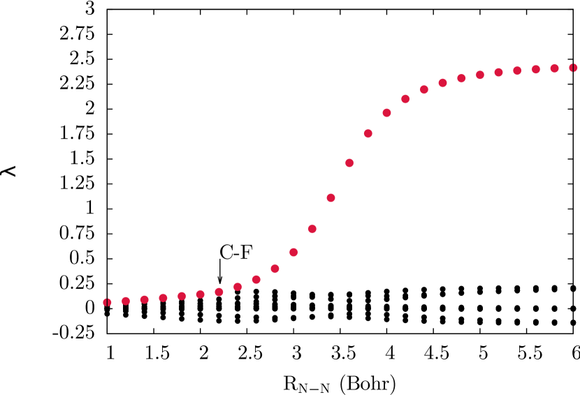
Figure 2: N₂ STO-3G eigenvalues of $U_{2}$ built from CCD amplitudes. Past the Coulson-Fischer point, a single large eigenvalue spin collective mode (shown in red) dominates.

Following our discussion of Fig. 2, and comparing Eqs. 29 and 31, we identify the largest eigenvalue of $U_{2}$ as the spin collective mode and write the collective and non-collective parts of $U_{2}$

$$U_{ai,bj}^{c} =\lambda_{\max}V_{ai,n_{\lambda_{\mathrm{max}}}}V_{bj,n_{\lambda_{\mathrm{max}}}},$$ (32a)

$$U_{ai,bj}^{nc} =U_{ai,bj}-U_{ai,bj}^{c}$$ (32b)

where $U^{c}$ and $U^{nc}$ refer to the collective- and noncollective blocks, respectively. Using Eqs. 32, we reconstruct $k_{ij}^{ab}$ amplitudes, i.e. CC amplitudes that want to mimic SUHF, and $s_{ij}^{ab}$ amplitudes, which are the rest of the CC amplitudes that simply capture weak correlation (compare to Eq. 16)

$$k_{ij}^{ab} =-\frac{1}{3}(U_{ai,bj}^{c}+2U_{aj,bi}^{c}),$$ (33a)

$$s_{ij}^{ab} =-\frac{1}{3}(U_{ai,bj}^{nc}+2U_{aj,bi}^{nc})=t_{ij}^{ab}-k_{ij}^{ab}.$$ (33b)

2.4 Computational Details

All calculations on the Hubbard and pairing Hamiltonians were performed using in-house code. The calculations on the Hubbard Hamiltonian all use periodic boundary condtions (PBC). Coupled cluster calculations on the Hubbard model use the RHF plane wave basis. Molecular Hartree-Fock and standard coupled cluster calculations were done in Gaussian 09,[43] while the attCC calculations were performed using in-house code. Standard extrapolation techniques are used to accelerate convergence.[44] Our calculations are done without point group symmetry. Thus, though we have $S=0$ SCF wavefunctions, they may break other symmetries, e.g. point group. Molecular bond lengths are in units of Bohr. We use cartesian $d$ functions and work in relatively small basis sets[45, 46] in order to exacerbate the effects of strong correlation and emphasize the deficiencies of standard coupled cluster in this regime.

3 Results

3.1 Molecules

We first test attCC on some small molecular systems. Results for the dissociation of N₂ in the STO-3G basis are shown in Fig. 3, where we plot total energies as function of bond length. As discussed earlier, the breakdown of CCSD is quite pronounced, as CCSD turns over near 3.2 bohr and overcorrelates dramatically at dissociation. As a result of the small basis, SUHF is exact at dissociation, but near equilibrium we can see that SUHF misses much of the dynamical correlation. In a sense, attCCSD offers the best of both worlds, giving energies comparable to CCSD near equilbrium and dissociating to the SUHF limit. Although there is a small bump in the attCCSD dissociation curve, it is qualitatively, and nearly quantitatively, correct.

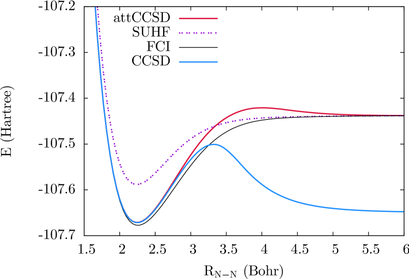
Figure 3: N₂ dissociation in STO-3G. CCSD overcorrelates dramatically at dissociation. SUHF dissociates correctly, but misses correlation at equilibrium. attCCSD captures correlation at both equilibrum and dissociation.

In Fig. 4, we plot the eigenvalues of $U_{2}$ (see Eq. 32), complementing Fig. 2. Here, $U_{2}$ is constructed with standard CSCD and attCCSD doubles amplitudes to show what happens to the spectrum after attenuation. For clarity, we have only shown the largest eigenvalue from CCSD. In the PoST formulation of SUHF, the eigenvalues are absorbed into the definition of $u$ in Eq. 29, so for SUHF in Fig. 4, we plot $u^{\dagger}u=\lambda$. The largest eigenvalue of attCC goes to the SUHF limit, and is unaffected by the addition of singles. The non-collective modes of attCC go to zero. Compared with Fig. 2, we see that the effect of attenuation in the strongly-correlated limit reproduces the spectrum of the SUHF wavefunction: the collective mode goes to SUHF, and the non-collective modes go to zero. This result also explains why attCC in general undercorrelates: when systems are too strongly-correlated, attCC looks too much like SUHF, and therefore lacks dynamic correlation. It is probable that residual dynamic correlation here originates from connected triples.

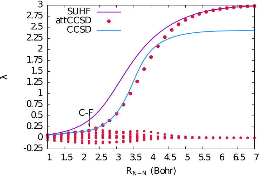
Figure 4: N₂ STO-3G eigenvalues of $U_{2}$. Attenuation gives the SUHF spectrum at dissociation.

Results for the symmetric dissociation of water with an H-O-H angle of $104.52\degree$[47] in the 3-21G basis are shown in Fig. 5, where we plot total energies as a function of the O-H bond length. We include single excitations, although results without singles are comparable in the minimal basis calculations shown here. At equilibrium, CCSD is very close to full configuration interaction (FCI), the exact result in this basis set. However, as the bond stretches, CCSD breaks down, turning over at around 4 bohr and overcorrelating at dissociation. CCSD0 is protected from breakdown, but sacrifices a large amount of dynamical correlation across all bond lengths. SUHF is well behaved throughout the curve, but also sacrifices dynamical correlation, particularly at equilibrium. At quilibrium, attCCSD is nearly identical with CCSD, giving energies better than SUHF in this regime. At dissociation, attCCSD is protected from the breakdown suffered by CCSD and gives energies superior to both CCSD0 and SUHF.

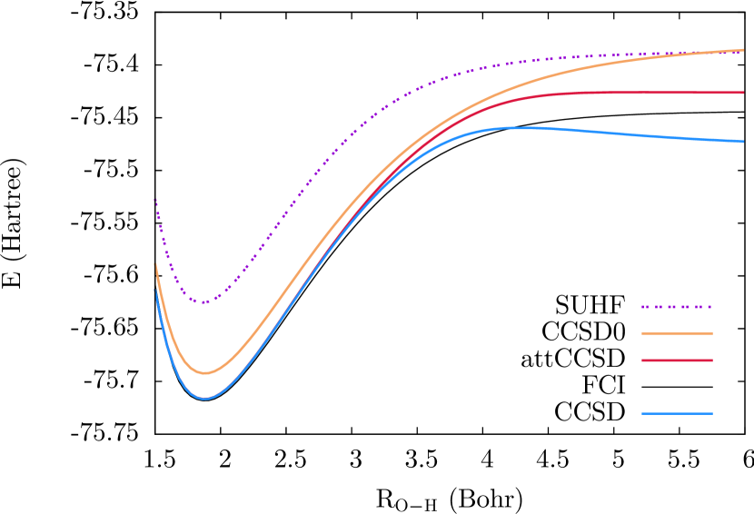
Figure 5: H₂O dissociation in 3-21G, $\theta_{\mathrm{H-O-H}}=104.52\degree$. CCSD overcorrelates at dissociation. CCSD0 and SUHF are well behaved but sacrifice dynamical correlation. attCCSD captures nearly all dynamical correlation at equilibrium and improves on SUHF and CCSD at dissociation.

Lastly, we look at the dissociation of N₂ in the larger cc-pVDZ basis[48] in Fig. 6. Calculations including singles and doubles are shown with solid lines; the corresponding doubles-only calculations are shown with dotted lines. The FCI results are all-electron, but use spherical $d$-functions, which raises the energy slightly. As in the minimal basis case, standard CC breaks down, turning over around 3.6 bohr and overcorrelating at dissociation. CC0 once again is protected from breakdown, but sacrifices dynamical correlation. SUHF gives the correct shape of the dissociation curve. However, there is more dynamical correlation in this larger basis. SUHF fails to capture this weak correlation, and gives poor energies overall. Once again, attCC gives excellent energies at equilibrium, is protected from breakdown at dissociation and improves on SUHF energies throughout the curve. However, even with the addition of singles, attCCSD misses a fair amount of correlation at dissociation, a failure we address in more detail in the Discussion section.

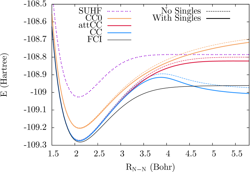
Figure 6: N₂ dissociation in cc-pVDZ. CC breaks down, overcorrelating at dissociation. CC0 is protected from breakdown, but misses weak correlation. SUHF has the correct shape, but misses weak correlation. attCCSD is accurate at equilibrium and improves on SUHF at dissociation, but still misses correlation from the intermediate region outward.

3.2 Hubbard

We now look at the 1-dimensional Hubbard model[49] at half filling with periodic boundary conditions (PBC). The Hamiltonian is given by

$$H=-t\sum\limits_{j,\sigma}(c^{\dagger}_{j+1,\sigma}c_{j,\sigma}+c^{\dagger}_{j,\sigma}c_{j+1,\sigma})+U\sum\limits_{j}n_{j\uparrow}n_{j\downarrow},$$ (34)

where $c^{\dagger}_{j,\sigma}$ and $c_{j,\sigma}$ create and annihilate an electron with spin $\sigma$ on site $j$, respectively, and $n_{j\sigma}=c^{\dagger}_{j,\sigma}c_{j,\sigma}$, the standard number operator for electrons of spin $\sigma$ on site $j$. The parameter $t$ allows electrons to hop between adjacent sites. The parameter $U>0$ represents repulsion of electrons on the same site. The model is well studied and loosely corresponds to a minimal basis chain of hydrogen atoms where the ratio $U/t$ is analogous to the interatomic bond distance. For large values of $U/t$, the system is strongly correlated. An attractive feature of the 1D Hubbard model with PBC is that exact results are available via a Bethe ansatz solution.[50, 51] RHF for this system yields plane waves, as opposed to the dimerized basis which is spin symmetry adapted, but translational symmetry broken. Due to momentum symmetry, single excitations are zero.

Results for the 6-site Hubbard model are shown in Fig. 7. For small values of $U/t$, CCD is essentially exact. However, CCD begins to overcorrelate near $U/t=4$, eventually turning over and heading toward negative infinity. Singlet-paired coupled cluster (CCD0), which we have found to be quite robust in molecular systems,[27, 34] is nearly exact for small values of $U/t$, but begins to plateau around $U/t=20$, eventually turning over. SUHF is well-behaved everywhere, but misses correlation throughout the curve, particularly for intermediate values of $U/t$. For small values of $U/t$, attCCD is nearly equivalent to CCD, and therefore superior to SUHF for $U/t\lesssim 5$. As a correction to CCD, attCCD at large values of $U/t$ is remarkable, as the relatively small modification we have made protects the method from breakdown. However, SUHF energies are much better than attCCD energies as $U/t$ becomes large.

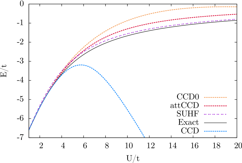
Figure 7: 6-site Hubbard in the plane-wave basis. Singles are zero by momentum symmetry. CCD breaks down, turning over around $U/t=6$. SUHF is good everywhere. attCCD improves over both CCD and CCD0.

Figs. 8 and 9 show results for 10- and 14-site Hubbard rings, respectively. The same qualitative features in our 6-site results are observed here as well. For small values of $U/t$, attCCD is quite accurate. As the system size increases, attCCD becomes less accurate at large values of $U/t$, relative to SUHF. However, as the system size increases, traditional CCD becomes progressively worse, turning over and failing to converge for smaller $U/t$. Although attCCD becomes less accurate as system size increases, it is also protected from the increasingly severe breakdown of CCD. We should note that SUHF is not size extensive and reverts to the same energy as UHF for large systems, an effect we seem to be seeing in the attCCD results.

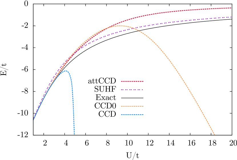
Figure 8: 10-site Hubbard. CCD breaks down, turning over sharply around $U/t=4$. CCD0 turns over around $U/t=8$. SUHF is good everywhere. attCCD improves dramatically over both CCD and CCD0.

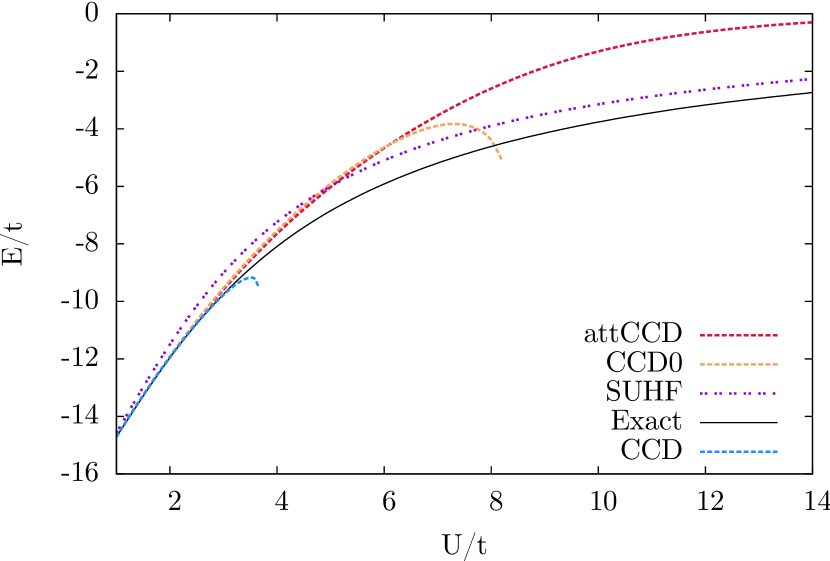
Figure 9: 14-site Hubbard. CCD breaks down, turning over sharply and becoming difficult to converge before $U/t=4$. CCD0 turns over around $U/t=7$ and stops converging at $U/t=8$. SUHF is reasonable everywhere. attCCD improves dramatically over both CCD and CCD0.

3.3 Pairing Attenuation

We have focused primarily on incorporating $S^{2}$ projection into CC in this work. However, we can combine CC with the projection of yet other symmetries, such as particle number. Particle number may be spontaneously broken in attractive Hamiltonians in analogy with the breaking of spin in repulsive Hamiltonians, but is more straight forward to attenuate than other repulsive Hamiltonian symmetries, e.g. $S_{z}$.

Consider the pairing or reduced BCS Hamiltonian, which is a simple model of superconductivity and is a good system to test our methods because it is very challenging for traditional coupled cluster:[52, 28]

$$H =\sum\limits_{p}\epsilon_{p}N_{p}-G\sum\limits_{p,q}P^{\dagger}_{p}P_{q},$$ (35a)

$$N_{p} =c^{\dagger}_{p\uparrow}c_{p\uparrow}+c^{\dagger}_{p\downarrow}c_{p\downarrow},$$ (35b)

$$P^{\dagger}_{p} =c^{\dagger}_{p\uparrow}c^{\dagger}_{p\downarrow},$$ (35c)

$$P_{p} =c_{p\uparrow}c_{p\downarrow}.$$ (35d)

Here, the sums are over single-particle levels of energy $\epsilon_{p}$ and the Hamiltonian has interaction strength $G$. As with 1D Hubbard, exact results are available.[53, 54] As $G$ increases, the HF reference tends toward a particle-number broken BCS solution at interactions $G$ larger than the critical point $G_{\mathrm{c}}$.

The number-projected wavefunction (PBCS) can be written as a Bessel polynomial of pair excitations out of the number-preserving Hartree-Fock reference[28]

$$\ket{\mathrm{PBCS}} =(1+T_{2}+\frac{1}{4}T_{2}^{2}+\frac{1}{36}T_{2}^{3}+...)\ket{0},$$ (36a)

$$T_{2} =t_{ii}^{aa}P^{\dagger}_{a}P_{i}.$$ (36b)

where the quadratic terms now carry a coefficient of $\frac{1}{4}$. Now, the pairing amplitudes factorize directly along particle-particle/hole-hole (pp-hh) lines as

$$t_{ii}^{aa}=x_{i}y^{a}.$$ (37)

Due to a symmetry of the Hamiltonian, $t_{ij}^{ab}=0$ if $i\neq j$ or $a\neq b$ for this system. Single and triple amplitudes are zero as well. Following the above procedure, we thus build

$$U_{ii,aa}=t_{ii}^{aa},$$ (38)

using the $t_{ij}^{ab}$ amplitudes from CCD. We then perform a singular value decomposition of $U_{ii,aa}$ along pp-hh lines and identify the largest singular value as the pairing collective mode. Going back to the CCD equations, we treat the terms quadratic in the pairing collective mode amplitudes with the coefficient of $\frac{1}{4}$ from the Bessel PBCS polynomial.

We show results for the 12-level pairing Hamiltonian in Fig. 10. Here, we plot the fraction of correlation energy recovered as a function of $G/G_{c}$. CCD is very accurate for small values of $G/G_{c}$, but overcorrelates drastically past the symmetry breaking point, eventually going complex.[52] Attenuated coupled cluster is comparable to CCD for small $G/G_{c}$. Although attCCD misses some correlation, especially in the intermediate region, it is protected from the breakdown of CCD.

As a comparison, we also show results from PoST Doubles,[28] which is a polynomial similarity transformation of double excitations that interpolates between CCD and PBCS. To do so, PoST Doubles gives $c_{2}=\frac{1}{2}$ (coupled cluster) for small $G$ in the pairing Hamiltonian and $c_{2}=\frac{1}{4}$ (PBCS) for large $G$, determining the value of $c_{2}$ by minimizing the quadruples $R_{4}$ residual.[28] Because it must minimize the $R_{4}$ residual, PoST Doubles has much higher computational scaling than attCCD and is difficult to apply to realistic systems. While the results for attCCD are not as good as those for PoST Doubles, attenuation is simpler and requires less computational effort.

Attenuated coupled cluster is not an interpolation, but applies the PBCS Bessel polynomial to one block of the amplitudes and the CC exponential polynomal to the the rest of the amplitudes (i.e. we apply the attenuation only in a ‘factorized’ eigenvector basis). It might be possible to make attCCD more in the spirit of PoST Doubles by introducing an interpolation scheme for the coefficient of the pairing collective mode, rather than applying a blanket $c_{2}=\frac{1}{4}$.

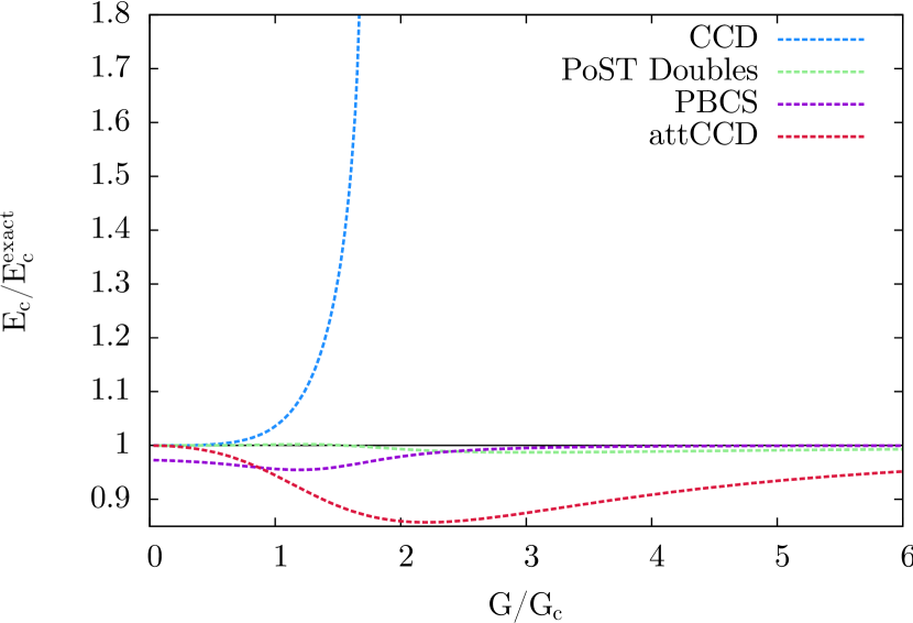
Figure 10: 12-site Pairing Hamiltonian. CCD overcorrelates, eventually going complex. PBCS is well behaved everywhere. attCCD is protected from breakdown at large $G$. PoST Doubles gives excellent results, but has much higher computational scaling than attCCD.

4 Discussion

In this work, we have demonstrated a simple method of combining the PoST singles formulation of spin symmetry projection with the exponential form of coupled cluster that has shown some promising initial results. In contrast with our previous work on singlet-paired coupled cluster, here we attenuate, rather than sever, the problematic interaction between channels in the CC equations, and do so along particle-hole/particle-hole lines instead of particle-particle/hole-hole lines as in Ref. [27].

It is important to emphasize that directly replacing the quadratic coefficient $c_{2}=\frac{1}{2}$ with $c_{2}=\frac{3}{10}$ and adding the unlinked terms in a CCD code does not give SUHF. As discussed above, such a procedure instead gives the projective equations

$$\braket{0}{\overline{H}_{\mathrm{PHF}}}{0} =E,$$ (39a)

$$\braket{{}_{ij}^{ab}}{\overline{H}_{\mathrm{PHF}}}{0} =0,$$ (39b)

which is manifestly not equal to the SUHF expectation value of Eq. 20, because of the inadequate bra state. We might refer to the method described in Eq. 39 as ‘projective’ SUHF (pSUHF), and it is equivalent to spin attenuating all modes of $t_{ij}^{ab}$, rather than just the collective mode attenuated in attCC. We have tested pSUHF, and though it is protected from breakdown due to strong correlation, like attCC, it gives worse energies. In a sense, the more the wavefunction can look like coupled cluster, withought reintroducing the breakdown, the better. To this end, attenuating only the spin collective mode seems superior to attenuating all modes. Indeed, we might be able to improve upon attCC by introducing an interpolation scheme for the coefficient of the spin collective mode, as described above for the pairing Hamiltonian. We are keenly interested in such a procedure, but determining how to optimize $c_{2}$ here is not straightforward.

Another shortcoming of attCC that will require some thought is the nature of the left-hand eigenvector. Currently, attCCD uses the projective coupled cluster-style amplitude and energy equations of Eq. 24. As PoST SUHF in Eq. 20 requires the left-hand eigenvector to produce the variational SUHF energy, a composite method of CC and SUHF may also need a more complicated left-hand side. The nature of such a formalism is the subject of ongoing work in our group, and we are optimistic about the promise of simultaneously describing weak and strong correlation with a combination of coupled cluster and symmery projection.

5 Acknowledgements

J.A.G. thanks Jacob Wahlen-Strothman for useful discussions, Dr. Matthias Degroote for help with the pairing Hamiltonian, Ethan Qiu for some of the exact results and Dr. Carlos Jiménez-Hoyos for his help with SUHF. This material is based on work supported by the National Science Foundation (CHE-1462434). G.E.S. is a Welch Foundation Chair (C-0036). J.A.G. gratefully acknowledges the support of the National Science Foundation Graduate Research Fellowship Program (DGE-1450681).

References

- [1] J. Paldus and X.A. Li, Adv. Chem. Phys 110, 1 (1999).
- [2] T.D. Crawford and H.F. Schaefer, in Reviews in Computational Chemistry (, , 2007), pp. 33–136.
- [3] R.J. Bartlett and M. Musial, Rev. Mod. Phys. 79, 291 (2007).
- [4] I. Shavitt and R.J. Bartlett, Many-Body Methods in Chemistry and Physics (Cambridge University Press, New York, NY, 2009).
- [5] P.O. Löwdin, Phys. Rev. 97, 1509 (1955).
- [6] P. Ring and P. Schuck, The Nuclear Many-Body Problem (Springer-Verlag, New York, NY, 1980).
- [7] J.P. Blaizot and G. Ripka, Quantum Theory of Finite Systems (The MIT Press, Cambridge, MA, 1986).
- [8] K. Schmid, Prog. Part. Nucl. Phys. 52, 564 (2004).
- [9] G.E. Scuseria, C.A. Jiménez-Hoyos, T.M. Henderson, J.K. Ellis and K. Samanta, J. Chem. Phys. 135, 124108 (2011).
- [10] C.A. Jiménez-Hoyos, T.M. Henderson, T. Tsuchimochi and G.E. Scuseria, J. Chem. Phys. 136, 164109 (2012).
- [11] Y. Qiu, T.M. Henderson and G.E. Scuseria (2017), In preparation.
- [12] J.M. Wahlen-Strothman, T.M. Henderson, M.R. Hermes, M. Degroote, Y. Qiu, J. Zhao, J. Dukelsky and G.E. Scuseria, J. Chem. Phys. (2017), in press.
- [13] Y. Qiu, T.M. Henderson and G.E. Scuseria, J. Chem. Phys. 145, 111102 (2016).
- [14] J. Paldus, J. Čížek and M. Takahashi, Phys. Rev. A 30, 2193 (1984).
- [15] P. Piecuch and J. Paldus, Theor. Chimica Acta 78, 65 (1990).
- [16] P. Piecuch, R. Toboła and J. Paldus, Phys. Rev. A. 54, 1210 (1996).
- [17] P. Piecuch, S.A. Kucharski and K. Kowalski, Chem. Phys. Lett. 344, 176 (2001).
- [18] R.J. Bartlett and M. Musial, J. Chem. Phys. 125, 204105 (2006).
- [19] F. Neese, F. Wennmohs and A. Hansen, J. Chem. Phys. 130, 114108 (2009).
- [20] L.M.J. Huntington and M. Nooijen, J. Chem. Phys. 133, 184109 (2010).
- [21] D.W. Small and M. Head-Gordon, J. Chem. Phys. 137, 114103 (2012).
- [22] D. Katz and F.R. Manby, J. Chem. Phys. 139, 021102 (2013).
- [23] P.A. Limacher, P.W. Ayers, P.A. Johnson, S. de Baerdemacker, D. Van Neck and P. Bultinck, J. Chem. Theor. Comp. 9, 1394 (2013).
- [24] T. Stein, T.M. Henderson and G.E. Scuseria, J. Chem. Phys 140, 214113 (2014).
- [25] T.M. Henderson, I.W. Bulik, T. Stein and G.E. Scuseria, J. Chem. Phys. 141, 244104 (2014).
- [26] T.M. Henderson, I.W. Bulik and G.E. Scuseria, J. Chem. Phys. 142, 214116 (2015).
- [27] I.W. Bulik, T.M. Henderson and G.E. Scuseria, J. Chem. Theor. Comp. 11, 3171 (2015).
- [28] M. Degroote, T.M. Henderson, J. Zhao, J. Dukelsky and G.E. Scuseria, Phys. Rev. B 79, 125124 (2016).
- [29] J.A. Gomez, T.M. Henderson and G.E. Scuseria, J. Chem. Phys. 144, 244117 (2016).
- [30] G.E. Scuseria, T.M. Henderson and I.W. Bulik, J. Chem. Phys. 139, 114110 (2013).
- [31] G.E. Scuseria, T.M. Henderson and D.C. Sorensen, J. Chem. Phys. 129, 231101 (2008).
- [32] G.E. Scuseria, C.L. Janssen and H.F. Schaefer III, J. Chem. Phys. 89, 7382 (1988).
- [33] G.E. Scuseria, A.C. Scheiner, T.J. Lee, J.E. Rice and H.F. Schaefer III, J. Chem. Phys. 86, 2881 (1987).
- [34] J.A. Gomez, T.M. Henderson and G.E. Scuseria, J. Chem. Phys. 145, 134103 (2016).
- [35] P.G. Szalay, M. Nooijen and R.J. Bartlett, J. Chem. Phys. 103, 281 (1995).
- [36] W. Kutzelnigg, Mol. Phys. 94, 65 (1998).
- [37] T. Van Voorhis and M. Head-Gordon, J. Chem. Phys. 113, 8873 (2000).
- [38] B. Cooper and P. Knowles, J. Chem. Phys. 133, 234102 (2010).
- [39] F. Evangelista, J. Chem. Phys. 134, 224102 (2011).
- [40] T. Tsuchimochi and T. Van Voorhis, J. Chem. Phys. 141, 164117 (2014).
- [41] T. Tsuchimochi, J. Chem. Phys. 143, 144114 (2015).
- [42] T. Tsuchimochi and S. Ten-No, J. Chem. Phys. 144, 11101 (2016).
- [43] M. Frisch, G.W. Trucks, H.B. Schlegel, G.E. Scuseria et al., Gaussian 09, Revision E.01 (Gaussian, Inc., Wallingford, CT, 2015).
- [44] G.E. Scuseria, T.J. Lee and H.F. Schaefer, Chem. Phys. Lett. 130, 236 (1986).
- [45] D.J. Feller, J. Comp. Chem. 17, 1571 (1996).
- [46] K.L. Schuchardt, B.T. Didier, T. Elsethagen, L. Sun, V. Gurumoorthi, J. Chase, J. Li and T.L. Windus, J. Chem. Inf. Model. 47, 1045 (2007).
- [47] L. Bytautas, G.E. Scuseria and K. Ruedenberg, J. Chem. Phys. 143, 094105 (2015).
- [48] T.H. Dunning, J. Chem. Phys. 90, 1070 (1989).
- [49] J. Hubbard, Proc. R. Soc. London, Ser. A 276, 238 (1963).
- [50] H. Bethe, Z. Phys. 71, 205 (1931).
- [51] E.H. Liebe and F.Y. Wu, Phys. Rev. Lett. 20, 1445 (1968).
- [52] T.M. Henderson, G.E. Scuseria, J. Dukelsky, A. Signoracci and T. Duguet, Phys. Rev. C 89, 054305 (2014).
- [53] R.W. Richardson, Phys. Rev. Lett. 3, 277 (1963).
- [54] R.W. Richardson, Phys. Rev. 141, 949 (1966).