Deterministic transfer of multiqubit GHZ entangled states and quantum secret sharing between different cavities

Abstract

We propose a way for transferring Greenberger-Horne-Zeilinger (GHZ) entangled states from $n$ qubits in one cavity onto another $n$ qubits in the other cavity. It is shown that $n$-qubit GHZ states $\alpha\left|00...0\right\rangle+\beta\left|11...1\right\rangle$ with arbitrary degree of entanglement can be transferred deterministically. Both of the GHZ state transfer and the operation time are not dependent on the number of qubits, and there is no need of measurement. This proposal is quite general and can be applied to accomplish the same task for a wide range of physical qubits. Furthermore, note that the $n$-qubit GHZ state $\alpha\left|00...0\right\rangle+\beta\left|11...1\right\rangle$ is a quantum-secret-sharing code for encoding a single-qubit arbitrary pure state $\alpha\left|0\right\rangle+\beta\left|1\right\rangle$. Thus, this work also provides a way to transfer quantum secret sharing from $n$ qubits in one cavity to another $n$ qubits in the other cavity.

I Introduction

Cavity-QED has been considered as one of the most powerful techniques for quantum information processing (QIP). During the past years, a great amount of work has been devoted to QIP with qubits coupled to (or placed in) a single cavity. Attention has been recently shifting to large-scale QIP based on cavity QED, which needs many qubits placed in different cavities. It is noted that placing all of qubits in a single cavity can cause many fundamental problems such as the increase in cavity decay rate and decrease in qubit-cavity coupling strength. Hence, future cavity-based QIP may require quantum networks consisting of multiple cavities, each hosting and coupled to multiple qubits. In this type of quantum network, transfer of quantum information will not only happen among qubits in the same cavity but also occur between different cavities.

Among a variety of multiqubit entangled states, Greenberger-Horne-Zeilinger (GHZ) states [1] are the archetype of multiqubit entangled states, which are especially of interest and have drawn considerable attention. They can be used to test nonlocality of quantum mechanics [1] and have applications in quantum metrology [2] and high-precision spectroscopy [3-5]. Moreover, GHZ states are useful in quantum teleportation [6,7], entanglement swapping [8], quantum cryptographic [9], and error correction protocols [10,11]. Over the past decade, based on cavity or circuit QED, a number of methods have been proposed for creating GHZ states with a wide range of physical systems such as atoms [12-14], quantum dots [15,16], superconducting (SC) qubits [17-20], and photons [21]. Moreover, experiments have demonstrated eight-photon GHZ states [22,23], fourteen-ion GHZ states [24], three-SC-qubit GHZ states (based on circuit QED) [25], five-SC-qubit GHZ states (via capacitance coupling) [26], and three-qubit GHZ states in NMR [27].

Quantum state transfer (QST) plays an essential role in quantum communication and is important in QIP. During the past decade, a great deal of efforts has been devoted to one-qubit QST, i.e., transferring an arbitrary unknown one-qubit state $\alpha\left|0\right\rangle+\beta\left|1\right\rangle$ ($\left|\alpha\right|^{2}+\left|\beta\right|^{2}=1$). Based on cavity/circuit QED, many theoretical proposals have been presented for implementing one-qubit QST in various physical systems [28-37], and one-qubit QST has been experimentally demonstrated with superconducting qubits [38,39] and spatially-separated atoms in a network [40]. Moreover, during the past years, much attention has been paid to quantum entanglement transfer (QET). Many proposals for implementing multi-qubit QET via quantum teleportation protocols have been presented [41-45], and schemes for realizing QET based on cavity QED or circuit QED have been also proposed [46-48]. Furthermore, QET has been experimentally demonstrated in linear optics [49,50].

Motivated by the above, we here consider a physical system consisting of two cavities each hosting $n$ qubits and coupled to a coupler qubit. In the following, we will propose a way to transfer an $n$-qubit GHZ state $\alpha\left|00...0\right\rangle+\beta\left|11...1\right\rangle$ (with arbitrary unknown coefficients $\alpha$ and $\beta$) from $n$ qubits in one cavity onto $n$ qubits in the other cavity. As shown below, this proposal has the following features and advantages: (i) The proposal can be used to implement the deterministic transfer of GHZ entangled states with arbitrary degree of entanglement, (ii) The GHZ state transfer does not depend on the number of qubits, (iii) The operation time does not increase as the number of qubits increases, (iv) No measurement is needed during the operation, (v) The level $\left|f\right\rangle$ of only two qubits is occupied during the operation, thus decoherence caused by energy relaxation and dephasing from the qubits is much suppressed, and (vi) This proposal is quite general and can be applied to a wide range of physical qubits such as atoms, quantum dots, NV centers and various superconducting qubits (e.g., phase, charge, flux, transmon, and Xmon qubits).

There are several additional motivations for this work, which are described below:

First, the transfer of multiqubit entangled states is not only fundamental in quantum mechanics but also important in QIP.

Second, multiqubit entangled states are essential resources for large-scale QIP. When qubits in the two cavities belong to the same species, transferring quantum entanglement is necessary in cavity-based large-scale QIP, which is performed across different information processors each consisting of a cavity and qubits in the cavity.

Third, when qubits in the two cavities are hybrid (i.e., different types), qubits in one cavity can act as information process cells (i.e., the operation qubits) while qubits in the other cavity play a role of quantum memory elements (i.e., the memory qubits). When performing QIP, after a step of information processing is completed, one may need to transfer quantum states (either entangled or non-entangled) of the operation qubits (i.e., SC qubits, which are readily controlled and used for performing quantum operations) to the memory qubits (i.e., NV centers [51] or atoms, which have long decoherence time) for storage; and one needs to transfer the quantum states from the memory qubits back to the operation qubits when a further step of processing is needed. Note that hybrid quantum systems, composed of different kinds of qubits (e.g., SC qubits and NV centers), have attracted tremendous attentions recently and are considered as promising candidates for QIP [52-55].

Last, according to [56], the $n$-qubit GHZ state $\alpha\left|00...0\right\rangle+\beta\left|11...1\right\rangle$ is a quantum-secret-sharing code, which encodes a single-qubit arbitrary pure state $\alpha\left|0\right\rangle+\beta\left|1\right\rangle$ via $n$ qubits. It is straightforward to see that after tracing over the other qubits, the density operator for each qubit is an identity $I,$ i.e., the original quantum information carried by a single qubit is uniformly distributed over $n$ qubits but each qubit does not carry any information. For the detailed discussion, see [56]. Hence, the method presented here also provides a way to transfer quantum secret sharing from $n$ qubits in one cavity to another $n$ qubits in the other cavity.

After a deep literature search, we note that based on cavity/circuit QED, how to transfer GHZ states between qubits distributed in different cavities and how to transfer quantum secret sharing between different cavities have not been reported.

This paper is outlined as follows. In Sec. II, we show a generic approach to transfer $n$-qubit GHZ entangled states from one cavity to the other cavity. In Sec. III, we give a brief discussion on the experimental issues. In Sec. IV, we discuss the experimental feasibility of transferring a three-qubit GHZ state in circuit QED. A concluding summary is given in Sec. V.

II Transferring multi-qubit GHZ-state between two cavities

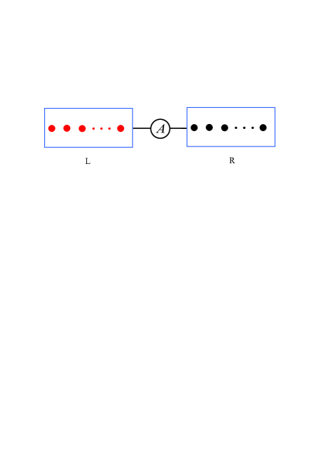
Figure 1: (Color online) Diagram of two sets of qubits placed in two different cavities connected to a coupler qubit. The circle $A$ in the middle represents the coupler qubit (e.g., a superconducting qubit or a quantum dot), which is capacitively or inductively coupled to each cavity. Each red or dark dot represents a qubit. The red dots represent qubits placed in the left cavity while the dark dots represent qubits placed in the right cavity. Qubits in the same cavity are identical but qubits in different cavities could be the same or non-identical (i.e., hybrid). In addition, each square box indicates a cavity, which could be a three-dimensional (3D) cavity or a one-dimensional (1D) cavity. The GHZ states of qubits in one cavity can be transferred onto qubits in the other cavity, as shown in the text.

Consider two cavities $L$ and $R$ coupled to a coupler qubit $A$ and each hosting $n$ qubits (Fig. 1). Without loss of generality, consider that qubits in the same cavity are identical (e.g., SC qubits) but qubits in different cavities are either the same or non-identity/hybrid (e.g., SC qubits in cavity $L$ while NV centers in cavity $R$). The $n$ qubits in cavity $L$ are labelled as $1,2,...,$ and $n$; while the $n$ qubits in cavity $R$ are denoted as $1^{\prime},2^{\prime},...,n^{\prime}$. For intra-cavity qubits, three levels $\left|g\right\rangle,$ $\left|e\right\rangle,$ and $\left|f\right\rangle$ are employed, while for the coupler qubit $A$ only two levels $\left|g\right\rangle_{A}$ and $\left|e\right\rangle_{A}$ are applied (Fig. 1). As shown below, the GHZ state transfer employs the qubit-cavity resonant interaction and the qubit-cavity dispersive interaction, which can be reached by adjusting the level spacings of qubits [57-63].

The qubits and the coupler qubit are initially decoupled from their respective cavities. Suppose that cavity $L$ ($R$) is initially in a vacuum state $\left|0\right\rangle_{L}$ $\left(\left|0\right\rangle_{R}\right)$, the coupler qubit is initially in the state $\left|g\right\rangle_{A}$, the $n$ qubits ($1,2,...,n$) in cavity $L$ are initially in a GHZ state

$$\left|GHZ\right\rangle_{12...n}=\alpha\left|g\right\rangle_{1}\prod_{l=2}^{n}\left|+\right\rangle_{l}+\beta\left|f\right\rangle_{1}\prod_{l=2}^{n}\left|-\right\rangle_{l}$$ (1)

(with unknown coefficients $\alpha$ and $\beta$), and the $n$ qubits ($1^{\prime},2^{\prime},...,n^{\prime}$) in cavity $R$ are initially in the state $\left|g\right\rangle_{1^{\prime}}\prod_{l^{\prime}=2^{\prime}}^{n^{\prime}}\left|+\right\rangle_{l^{\prime}}.$ Here, $\left|\pm\right\rangle=\left(\left|g\right\rangle\pm\left|e\right\rangle\right)/\sqrt{2}$ are two orthogonal states. The initial state of the whole system is thus given by

$$\left(\alpha\left|g\right\rangle_{1}\prod_{l=2}^{n}\left|+\right\rangle_{l}+\beta\left|f\right\rangle_{1}\prod_{l=2}^{n}\left|-\right\rangle_{l}\right)\otimes\left|g\right\rangle_{A}\otimes\left|g\right\rangle_{1^{\prime}}\prod_{l^{\prime}=2^{\prime}}^{n^{\prime}}\left|+\right\rangle_{l^{\prime}}\otimes\left|0\right\rangle_{L}\left|0\right\rangle_{R}.$$ (2)

In the following, the Hamiltonians are written in the interaction picture, $a^{+}$ ($b^{+}$) is the photon creation operator of cavity $L$ ($R$), and $\omega_{a\text{ }}$($\omega_{b}$) is the frequency of cavity $L$ ($R$). The whole procedure for transferring the GHZ state of the $n$ qubits ($1,2,...,n$) in cavity $L$ onto the $n$ qubits ($1^{\prime},2^{\prime},...,n^{\prime}$) in cavity $R$ is listed below:

Step 1: Adjust the level spacings of qubit 1 to bring the $\left|e\right\rangle\leftrightarrow\left|f\right\rangle$ transition on resonance with cavity $L$ [Fig. 2(a)]. The Hamiltonian is given by $H_{1,1}=\hbar\left(\mu_{1}a^{+}\left|e\right\rangle_{1}\left\langle f\right|+h.c.\right),$ where $\mu_{1}$ is the resonant coupling strength between cavity $L$ and the $\left|e\right\rangle\leftrightarrow\left|f\right\rangle$ transition of qubit 1. Under the Hamiltonian $H_{1,1}$ and after an interaction time $t_{1,1}=\pi/\left(2\mu_{1}\right),$ the state component $\left|f\right\rangle_{1}\left|0\right\rangle_{L}$ changes to $-i\left|e\right\rangle_{1}\left|1\right\rangle_{L}$ (for the details, see [64]). Now adjust the level spacings of qubit $1$ to bring the $\left|g\right\rangle\leftrightarrow\left|e\right\rangle$ transition on resonance with cavity $L$ [Fig. 2(b)]. The Hamiltonian is $H_{1,2}=\hbar\left(\widetilde{\mu}_{1}a^{+}\left|g\right\rangle_{1}\left\langle e\right|+h.c.\right),$ with $\widetilde{\mu}_{1}$ being the resonant coupling strength between cavity $L$ and the $\left|g\right\rangle\leftrightarrow\left|e\right\rangle$ transition of qubit 1. Under the Hamiltonian $H_{1,2}$ and after an interaction time $t_{1,2}=\pi/\left(2\sqrt{2}\widetilde{\mu}_{1}\right),$ the state component $\left|e\right\rangle_{1}\left|1\right\rangle_{L}$ changes to $-i\left|g\right\rangle_{1}\left|2\right\rangle_{L}$ [64].

After this step of operation, we can obtain the transformation $\left|f\right\rangle_{1}\left|0\right\rangle_{L}\rightarrow-\left|g\right\rangle_{1}\left|2\right\rangle_{L}$ but the state component $\left|g\right\rangle_{1}\left|0\right\rangle_{L}$ remains unchanged because of $H_{1,1}\left|g\right\rangle_{1}\left|0\right\rangle_{L}=H_{1,2}\left|g\right\rangle_{1}\left|0\right\rangle_{L}=0.$ Thus, the initial state (2) of the whole system becomes

$$\left|g\right\rangle_{1}\left(\alpha\prod_{l=2}^{n}\left|+\right\rangle_{l}\left|0\right\rangle_{L}-\beta\prod_{l=2}^{n}\left|-\right\rangle_{l}\left|2\right\rangle_{L}\right)\otimes\left|g\right\rangle_{A}\otimes\left|g\right\rangle_{1^{\prime}}\prod_{l^{\prime}=2^{\prime}}^{n^{\prime}}\left|+\right\rangle_{l^{\prime}}\otimes\left|0\right\rangle_{R}.$$ (3)

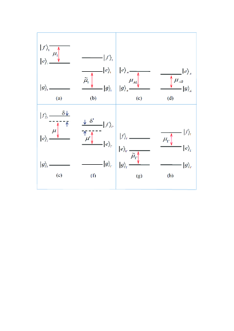
Figure 2: (Color online) Illustration of qubit-cavity interaction. (a) Resonant interaction between cavity $L$ with the $\left|e\right\rangle\leftrightarrow\left|f\right\rangle$ transition of qubit 1. (b) Resonant interaction between cavity $L$ with the $\left|g\right\rangle\leftrightarrow\left|e\right\rangle$ transition of qubit 1. (c) Resonant interaction between cavity $L$ with the $\left|g\right\rangle\leftrightarrow\left|e\right\rangle$ transition of the coupler qubit $A$. (d) Resonant interaction between cavity $R$ with the $\left|g\right\rangle\leftrightarrow\left|e\right\rangle$ transition of the coupler qubit $A$. (e) Dispersive interaction between cavity $L$ and the $\left|e\right\rangle\leftrightarrow\left|f\right\rangle$ transition of qubits ($2,3,...,n$). In (e), the subscript $l=2,3,...,n$. (f) Dispersive interaction between cavity $R$ and the $\left|e\right\rangle\leftrightarrow\left|f\right\rangle$ transition of qubits ($2^{\prime},3^{\prime},...,n^{\prime}$). In (f), the subscript $l^{\prime}=2^{\prime},3^{\prime},...,n^{\prime}$. (g) Resonant interaction between cavity $R$ and the $\left|g\right\rangle\leftrightarrow\left|e\right\rangle$ transition of qubit $1^{\prime}$. (h) Resonant interaction between cavity $R$ and the $\left|e\right\rangle\leftrightarrow\left|f\right\rangle$ transition of qubit $1^{\prime}$. When going from (a) to (h), the level spacings of qubits and the coupler qubit need to be adjusted to obtain the required qubit-cavity resonant or dispersive interaction. Note that the level spacings of qubits and the coupler qubit can be readily adjusted by varying the external control parameters or control fields (see, [57-63]). In (a-h), each vertical blue-color arrow line indicates the mode frequency of cavity $L$, while each vertical red-color arrow line represents the mode frequency of cavity $R$.

Step 2: Adjust the level spacings of qubit $1$ back to the previous situation such that cavity $L$ is decoupled from this qubit. In the meantime, bring the coupler qubit $A$ on resonance with cavity $L$ [Fig. 2(c)]. The Hamiltonian is $H_{2,1}=\hbar\left(\mu_{AL}a^{+}\left|g\right\rangle_{A}\left\langle e\right|+h.c.\right),$ where $\mu_{AL}$ is the resonant coupling strength between cavity $L$ and the coupler qubit $A$. Under the Hamiltonian $H_{2,1}$ and after an interaction time $t_{2,1}=\pi/\left(2\sqrt{2}\mu_{AL}\right),$ the state component $\left|g\right\rangle_{A}\left|2\right\rangle_{L}$ changes to $-i\left|e\right\rangle_{A}\left|1\right\rangle_{L}$ [64]. Now bring the coupler qubit $A$ on resonance with cavity $R$ [Fig. 2(d)]. The Hamiltonian is $H_{2,2}=\hbar\left(\mu_{AR}b^{+}\left|g\right\rangle_{A}\left\langle e\right|+h.c.\right),$ where $\mu_{AR}$ is the resonant coupling strength between cavity $R$ and the coupler qubit $A$. Under the Hamiltonian $H_{2,2}$ and after an interaction time $t_{2,2}=\pi/\left(2\mu_{AR}\right),$ the state component $\left|e\right\rangle_{A}\left|1\right\rangle_{L}\left|0\right\rangle_{R}$ changes to $-i\left|g\right\rangle_{A}\left|1\right\rangle_{L}\left|1\right\rangle_{R}.$

After this step of operation, we can obtain the transformation $\left|g\right\rangle_{A}\left|2\right\rangle_{L}\left|0\right\rangle_{R}\rightarrow-\left|g\right\rangle_{A}\left|1\right\rangle_{L}\left|1\right\rangle_{R}$ but the state component $\left|g\right\rangle_{A}\left|0\right\rangle_{L}\left|0\right\rangle_{R}$ remains unchanged due to $H_{2,1}\left|g\right\rangle_{A}\left|0\right\rangle_{L}\left|0\right\rangle_{R}=H_{2,2}\left|g\right\rangle_{A}\left|0\right\rangle_{L}\left|0\right\rangle_{R}=0.$ Hence, the state (3) becomes

$$\left|g\right\rangle_{1}\left(\alpha\prod_{l=2}^{n}\left|+\right\rangle_{l}\left|0\right\rangle_{L}\left|0\right\rangle_{R}+\beta\prod_{l=2}^{n}\left|-\right\rangle_{l}\left|1\right\rangle_{L}\left|1\right\rangle_{R}\right)\otimes\left|g\right\rangle_{A}\otimes\left|g\right\rangle_{1^{\prime}}\prod_{l^{\prime}=2^{\prime}}^{n^{\prime}}\left|+\right\rangle_{l^{\prime}}.$$ (4)

Step 3: Bring the coupler qubit $A$ back to the original level configuration such that the qubit $A$ is decoupled from the two cavities. Meanwhile, adjust the level spacings of qubits ($2,3,...,n$) to have their $\left|e\right\rangle\leftrightarrow\left|f\right\rangle$ transition coupled to cavity $L$ [Fig. 2(e)], and adjust the level spacings of qubits ($2^{\prime},3^{\prime},...,n)$] to have their $\left|e\right\rangle\leftrightarrow\left|f\right\rangle$ transition coupled to cavity $R$ [Fig. 2(f)]. The interaction Hamiltonian is given by

$$H=\sum_{l=2}^{n}\mu\left(e^{i\delta t}a\left|f\right\rangle_{l}\left\langle e\right|+h.c.\right)+\sum_{l^{\prime}=2^{\prime}}^{n^{\prime}}\mu^{\prime}\left(e^{i\delta^{\prime}t}b\left|f\right\rangle_{l^{\prime}}\left\langle e\right|+h.c.\right),$$ (5)

where $\delta$$=\omega_{fe}-\omega_{a\text{ }},$ $\delta^{\prime}$$=\omega_{fe}^{\prime}-\omega_{b\text{ }},$ and $\mu$ ($\mu^{\prime}$) is the non-resonant (dispersive) coupling strength between cavity $L$ ($R$) and the $\left|e\right\rangle\leftrightarrow\left|f\right\rangle$ transition of qubits ($2,3,...,n$) [qubits ($2^{\prime},3^{\prime},...,n)$]. Here, $\omega_{fe}$ ($\omega_{fe}^{\prime}$) is the $\left|e\right\rangle$ $\leftrightarrow$ $\left|f\right\rangle$ transition frequency for qubits ($2,3,...,n$) [qubits ($2^{\prime},3^{\prime},...,n^{\prime})$].

Under the large detuning condition $\delta\gg\mu$ and $\delta^{\prime}\gg\mu^{\prime},$ we can obtain the following effective Hamiltonian [65,66]

$$H = \lambda\sum\limits_{l=2}^{n}\left(\left|f\right\rangle_{l}\left\langle f\right|aa^{+}-\left|e\right\rangle_{l}\left\langle e\right|a^{+}a\right)$$ (6)

$$+\lambda^{\prime}\sum\limits_{l^{\prime}=2^{\prime}}^{n^{\prime}}\left(\left|f\right\rangle_{l^{\prime}}\left\langle f\right|bb^{+}-\left|e\right\rangle_{l^{\prime}}\left\langle e\right|b^{+}b\right)$$

$$+\lambda\sum_{l\neq k=2}^{n}\left|f\right\rangle_{l}\left\langle e\right|\otimes\left|e\right\rangle_{k}\left\langle f\right|$$

$$+\lambda^{\prime}\sum_{l^{\prime}\neq k^{\prime}=2}^{n}\left|f\right\rangle_{l^{\prime}}\left\langle e\right|\otimes\left|e\right\rangle_{k^{\prime}}\left\langle f\right|,$$

where $\lambda=\mu^{2}/\delta$ and $\lambda^{\prime}=\left(\mu^{\prime}\right)^{2}/\delta^{\prime}$ are the effective coupling strengths. The terms in lines 1 and 2 of Eq. (6) describe the photon-number dependent Stark shifts. The term in line 3 describes the “dipole” couplings between the $l$th qubit and the $k$th qubit (in cavity $L$), and the term in the last line describes the “dipole” couplings between the $l^{\prime}$th qubit and the $k^{\prime}$th qubit (in cavity $R$). Note that the level $\left|f\right\rangle$ of each qubit is not involved in the state (4). Thus, one can easily find that only the terms $-\lambda\sum\limits_{l=2}^{n}\left|e\right\rangle_{l}\left\langle e\right|a^{+}a$ and $-\lambda^{\prime}\sum\limits_{l^{\prime}=2^{\prime}}^{n^{\prime}}\left|e\right\rangle_{l^{\prime}}\left\langle e\right|b^{+}b$ of Eq. (6) have contribution to the time evolution of the state (4), while all other terms in Eq. (6) acting on the state (4) result in zero. In other words, with respective to the state (4), the Hamiltonian (6) reduces to

$$H=-\lambda\sum\limits_{l=2}^{n}\left|e\right\rangle_{l}\left\langle e\right|a^{+}a-\lambda^{\prime}\sum\limits_{l=2^{\prime}}^{n^{\prime}}\left|e\right\rangle_{l^{\prime}}\left\langle e\right|b^{+}b.$$ (7)

Under the Hamiltonian (7), the state (4) evolves into

$$\left|g\right\rangle_{1}\left(\alpha\prod_{l=2}^{n}\left|+\right\rangle_{l}\prod_{l^{\prime}=2^{\prime}}^{n^{\prime}}\left|+\right\rangle_{l^{\prime}}\left|0\right\rangle_{L}\left|0\right\rangle_{R}\right.+$$

$$\left.+\beta\prod_{l=2}^{n}\left(\left|g\right\rangle_{l}-e^{i\lambda t}\left|e\right\rangle_{l}\right)\prod_{l^{\prime}=2^{\prime}}^{n^{\prime}}\left(\left|g\right\rangle_{l^{\prime}}+e^{i\lambda^{\prime}t}\left|e\right\rangle_{l^{\prime}}\right)\left|1\right\rangle_{L}\left|1\right\rangle_{R}\right)$$

$$\otimes\left|g\right\rangle_{A}\otimes\left|g\right\rangle_{1^{\prime}}.$$ (8)

In the case of $t_{3}=\left(2m+1\right)\pi/\lambda=\left(2k+1\right)\pi/\lambda^{\prime}$ ($m$ and $k$ are zero or positive integers), we have from Eq. (8)

$$\left|g\right\rangle_{1}\prod_{l=2}^{n}\left|+\right\rangle_{l}\left(\alpha\prod_{l^{\prime}=2^{\prime}}^{n^{\prime}}\left|+\right\rangle_{l^{\prime}}\left|0\right\rangle_{L}\left|0\right\rangle_{R}+\beta\prod_{l^{\prime}=2^{\prime}}^{n^{\prime}}\left|-\right\rangle_{l^{\prime}}\left|1\right\rangle_{L}\left|1\right\rangle_{R}\right)\otimes\left|g\right\rangle_{A}\otimes\left|g\right\rangle_{1^{\prime}}.$$ (9)

Step 4: Adjust the level structure of qubits ($2,3,...,n$) and qubits ($2^{\prime},3^{\prime},...,n^{\prime}$) back to the previous configuration while bring the coupler qubit $A$ on resonance with cavity $L$ [Fig. 2(c)]. The Hamiltonian is given by $H_{2,1}$ above. Under the Hamiltonian $H_{2,1}$ and after an interaction time $t_{4,1}=\pi/\left(2\mu_{AL}\right),$ the state component $\left|g\right\rangle_{A}\left|1\right\rangle_{L}\left|1\right\rangle_{R}$ changes to $-i\left|e\right\rangle_{A}\left|0\right\rangle_{L}\left|1\right\rangle_{R}$. Then, bring the coupler qubit $A$ on resonance with cavity $R$ [Fig. 2(d)]. The Hamiltonian is given by $H_{2,2}$ above. Under the Hamiltonian $H_{2,2}$ and after an interaction time $t_{4,4}=\pi/\left(2\sqrt{2}\mu_{AR}\right),$ the state component $\left|e\right\rangle_{A}\left|0\right\rangle_{L}\left|1\right\rangle_{R}$ changes to $-i\left|g\right\rangle_{A}\left|0\right\rangle_{L}\left|2\right\rangle_{R}.$

After the operation of this step, we can get the transformation $\left|g\right\rangle_{A}\left|1\right\rangle_{L}\left|1\right\rangle_{R}\rightarrow-\left|g\right\rangle_{A}\left|0\right\rangle_{L}\left|2\right\rangle_{R}$ but the state component $\left|g\right\rangle_{A}\left|0\right\rangle_{L}\left|0\right\rangle_{R}$ remains unchanged. Hence, the state (9) becomes

$$\left|g\right\rangle_{1}\prod_{l=2}^{n}\left|+\right\rangle_{l}\otimes\left|g\right\rangle_{A}\otimes\left|0\right\rangle_{L}\otimes\left(\alpha\prod_{l^{\prime}=2^{\prime}}^{n^{\prime}}\left|+\right\rangle_{l^{\prime}}\left|0\right\rangle_{R}-\beta\prod_{l^{\prime}=2^{\prime}}^{n^{\prime}}\left|-\right\rangle_{l^{\prime}}\left|2\right\rangle_{R}\right)\otimes\left|g\right\rangle_{1^{\prime}}.$$ (10)

Step 5: Bring the coupler qubit $A$ back to the original level configuration such that it is decoupled from the two cavities. Meanwhile, adjust the level spacings of qubit $1^{\prime}$ such that the $\left|g\right\rangle\leftrightarrow\left|e\right\rangle$ transition of qubit $1^{\prime}$ is resonant with cavity $R$ [Fig. 2(g)]. The Hamiltonian is $H_{5,1}=\hbar\left(\widetilde{\mu}_{1^{\prime}}b^{+}\left|g\right\rangle_{1^{\prime}}\left\langle e\right|+h.c.\right),$ where $\widetilde{\mu}_{1^{\prime}}$ is the resonant coupling strength between cavity $R$ and the $\left|g\right\rangle\leftrightarrow\left|e\right\rangle$ transition of qubit $1^{\prime}$. Under the Hamiltonian $H_{5,1}$ and after an interaction time $t_{5,1}=\pi/\left(2\sqrt{2}\widetilde{\mu}_{1^{\prime}}\right),$ the state component $\left|g\right\rangle_{1^{\prime}}\left|2\right\rangle_{R}$ changes to $-i\left|e\right\rangle_{1^{\prime}}\left|1\right\rangle_{R}$. Adjust the level spacings of qubit $1^{\prime}$ so that the $\left|e\right\rangle\leftrightarrow\left|f\right\rangle$ transition of qubit $1^{\prime}$ is resonant with cavity $R$ [Fig. 2(h)]. The Hamiltonian is given by $H_{5,2}=\hbar\left(\mu_{1^{\prime}}b^{+}\left|e\right\rangle_{1^{\prime}}\left\langle f\right|+h.c.\right),$ with $\mu_{1^{\prime}}$ being the resonant coupling strength between cavity $R$ and the $\left|e\right\rangle\leftrightarrow\left|f\right\rangle$ transition of qubit $1^{\prime}$. Under this Hamiltonian and after an interaction time $t_{5,2}=\pi/\left(2\widetilde{\mu}_{1^{\prime}}\right),$ the state component $\left|e\right\rangle_{1^{\prime}}\left|1\right\rangle_{R}$ changes to $-i\left|f\right\rangle_{1^{\prime}}\left|0\right\rangle_{R}.$

After performing this step of operation, we can get the transformation $\left|g\right\rangle_{1^{\prime}}\left|2\right\rangle_{R}\rightarrow-\left|f\right\rangle_{1^{\prime}}\left|0\right\rangle_{R}$ but the state component $\left|g\right\rangle_{1^{\prime}}\left|0\right\rangle_{R}$ remains unchanged because of $H_{5,1}\left|g\right\rangle_{1^{\prime}}\left|0\right\rangle_{R}=H_{5,2}\left|g\right\rangle_{1^{\prime}}\left|0\right\rangle_{R}=0.$ Thus, the state (10) of the whole system becomes

$$\left|g\right\rangle_{1}\prod_{l=2}^{n}\left|+\right\rangle_{l}\otimes\left|g\right\rangle_{A}\otimes\left|0\right\rangle_{L}\left|0\right\rangle_{R}\otimes\left(\alpha\left|g\right\rangle_{1^{\prime}}\prod_{l^{\prime}=2^{\prime}}^{n^{\prime}}\left|+\right\rangle_{l^{\prime}}+\beta\left|f\right\rangle_{1^{\prime}}\prod_{l^{\prime}=2^{\prime}}^{n^{\prime}}\left|-\right\rangle_{l^{\prime}}\right).$$ (11)

After the operation, the level spacings of qubit $1^{\prime}$ needs to be adjusted such that qubit $1^{\prime}$ is decoupled from cavity $R$.

Note that the last part of the product in Eq. (11) is the state of qubits ($1^{\prime},2^{\prime},...,n^{\prime}$), which is the same as the GHZ state of qubits ($1,2,...,n$), described by Eq. (1). Thus, the original $n$-qubit GHZ state of qubits ($1,2,...,n$) in cavity $L$ has been transferred onto qubits ($1^{\prime},2^{\prime},...,n^{\prime}$) in cavity $R$ after the above operations. By applying classical pulse to qubit $1^{\prime},$ the states $\left|g\right\rangle_{1^{\prime}}$ and $\left|f\right\rangle_{1^{\prime}}$ can be easily converted into the states $\left|+\right\rangle_{1^{\prime}}$ and $\left|-\right\rangle_{1^{\prime}}$, respectively.

The irrelevant qubits in each step described above need to be decoupled from their respective cavities. This requirement can be achieved by the adjustment of the level spacings of the qubits. For example, (i) The level spacings of superconducting qubits can be rapidly adjusted by varying external control parameters (e.g. the magnetic flux applied to a superconducting loop of phase, transmon, Xmon or flux qubits; see e.g. [57-60]); (ii) The level spacings of NV centers can be readily adjusted by changing the external magnetic field applied along the crystalline axis of each NV center [61,62]; and (iii) The level spacings of atoms/quantum dots can be adjusted by changing the voltage on the electrodes around each atom/quantum dot [63].

Additional points may need to be addressed. First, because the same detuning $\delta$ ($\delta^{\prime}$) is set for qubits ($2,3,...,n$) [qubits ($2^{\prime},3^{\prime},...,n^{\prime}$)], the level spacings for qubits ($2,3,...,n$) [qubits ($2^{\prime},3^{\prime},...,n^{\prime}$)] can be synchronously adjusted, e.g., via changing the common external control parameters. Second, as shown above, the level $\left|f\right\rangle$ for qubits ($2,3,...,n$) and qubits ($2^{\prime},3^{\prime},...,n^{\prime}$) is unpopulated, i.e., the level $\left|f\right\rangle$ is occupied only for two qubits $1$ and $1^{\prime}$ ; thus decoherence from $2n-2$ qubits out of $2n$ qubits is greatly suppressed during the entire operation. Third, the operation has nothing to do with $\alpha$ and $\beta,$ thus GHZ states with arbitrary degree of entanglement can be transferred by using this proposal. Last, the method is applicable to 1D, 2D or 3D cavities or resonators as long as the conditions described above are met.

Before ending this section, it should be pointed out that all above-mentioned qubit-cavity resonant interactions involved during the GHZ state transfer can be completed within a very short time, e.g., by increasing the qubit-cavity resonant coupling strengths.

III Disscussion

For the method to work, the following requirements need to be satisfied:

(i) The condition $\left(2m+1\right)\pi/\lambda=\left(2k+1\right)\pi/\lambda^{\prime}$ needs to be met. Because of $\lambda=\mu^{2}/\delta$ and $\lambda^{\prime}=\left(\mu^{\prime}\right)^{2}/\delta^{\prime},$ this condition can be readily reached with an appropriate choice of $\delta$ (or $\delta^{\prime}$) via adjusting the level spacings of qubits ($2,3,...,n$) [or qubits ($2^{\prime},3^{\prime},...,n^{\prime}$)]. For the case when qubits in the two cavities belong to the same species and the two cavities are identical, one would have $\lambda=\lambda^{\prime}$ (i.e., $\delta=\delta^{\prime}$ and $\mu=\mu^{\prime}$) and thus could choose $m=k=0$ to have $\tau_{5}=\pi/\lambda=\pi/\lambda^{\prime}$, i.e., the shortest operation time for step 3.

(ii) During step 3, the occupation probability $p$ of the level $\left|f\right\rangle$ for each of qubits ($2,3,...,n$) and the occupation probability $p^{\prime}$ of the level $\left|f\right\rangle$ for each of qubits ($2^{\prime},3^{\prime},...,n^{\prime}$) are given by [67,68]

$$p\simeq\frac{4\mu^{2}}{4\mu^{2}+\delta^{2}},\text{ }p^{\prime}\simeq\frac{4\left(\mu^{\prime}\right)^{2}}{4\left(\mu^{\prime}\right)^{2}+(\delta^{\prime})^{2}}.$$ (12)

The occupation probabilities $p$ and $p^{\prime}$ need to be negligibly small in order to reduce the operation error. With the choice of $\delta=10\mu$ and $\delta^{\prime}=10\mu^{\prime},$ one has $p,$ $p^{\prime}\sim 0.04$, which can be further reduced by increasing the ratio of $\delta/\mu$ and $\delta^{\prime}/\mu^{\prime}.$

(iii) The total operation time is

$$\tau=\tau_{r}+\tau_{o}+\tau_{a},$$ (13)

with

$$\tau_{r} = \frac{\pi}{2}\left(\mu_{1}^{-1}+\mu_{1^{\prime}}^{-1}+\mu_{AL}^{-1}+\mu_{AR}^{-1}\right)+\frac{\pi}{2\sqrt{2}}\left(\widetilde{\mu}_{1}^{-1}+\widetilde{\mu}_{1^{\prime}}^{-1}+\mu_{AL}^{-1}+\mu_{AR}^{-1}\right),$$ (14)

$$\tau_{o} = \left(2m+1\right)\pi/\lambda=\left(2k+1\right)\pi/\lambda^{\prime},$$ (15)

$$\tau_{a} = 6\tau_{A}+3\tau_{1}+3\tau_{1^{\prime}}+2\tau_{q}+2\tau_{q^{\prime}}.$$ (16)

Here, $\tau_{r}$ is a total of resonance operation time for steps 1, 2, 4, and 5; $\tau_{o}$ is the off-resonance operation time for step 3; and $\tau_{a}$ is a total of time required for adjusting the level spacings of the qubits and the coupler qubit. In addition, $\tau_{1},$ $\tau_{1^{\prime}},$ and $\tau_{A}$ are the typical times needed for adjusting the level spacings of qubit 1, qubit $1^{\prime},$ and the coupler qubit $A$, respectively; $\tau_{q}$ ($\tau_{q^{\prime}}$) is the typical time required for adjusting the level spacings of qubits ($2,3,...,n$) [qubits ($1^{\prime},2^{\prime},...,n^{\prime}$)].

From Eqs. (13-16), one can see that the operation time $\tau$ is independent of the number of qubits. To reduce decoherence, the operation time $\tau$ should be much smaller than the energy relaxation time and the dephasing time of qubits. In addition, $\tau$ should be much smaller than the lifetime of the cavity mode, which is given by $\kappa_{j}^{-1}=Q_{j}/\omega_{j}$ ($j=a,b$). Here, $Q_{a}$ ($Q_{b}$) is the quality factor of cavity $L$ ($R$). In principle, these requirements can be satisfied. The $\tau_{r}$ can be reduced by increasing the resonant coupling strengths $\mu_{1},\widetilde{\mu}_{1},\mu_{1^{\prime}},\widetilde{\mu}_{1^{\prime}},\mu_{AL},$ and $\mu_{AR}.$ The $\tau_{a}$ can be reduced by rapidly adjusting the level spacings of the qubits and the coupler qubit (e.g., $1-3$ ns is the typical time for adjusting the level spacings of superconducting qubits in experiment [69,70]). And, $\kappa^{-1}$ can be increased by employing high-$Q$ cavities.

IV Possible experimental implementation

As an example, let us give a discussion of the experimental possibility of transferring a three-qubit GHZ state from three identical superconducting transmon qubits in one cavity to another three identical superconducting transmon qubits in the other cavity (Fig. 3). Each cavity considered here is a one-dimensional transmission line resonator (TLR), and the two cavities are coupled to a superconducting transmon qubit (Fig. 3).

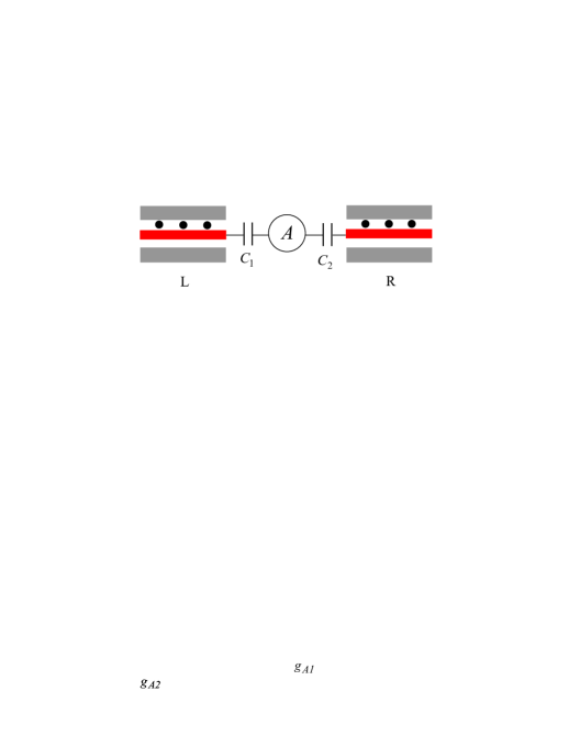
Figure 3: (Color online) Setup for two cavities $L$ and $R$ coupled by a superconducting transmon qubit $A$. Each cavity here is a one-dimensional coplanar waveguide transmission line resonator. The circle $A$ represents a superconducting transmon qubit (i.e., an artificial atom), which is capacitively coupled to cavity $L$ ($R$) via a capacitance $C_{1}$ ($C_{2}$). Each dark dot indicate an intra-cavity superconducting transmon qubit.

Assume $\widetilde{\mu}_{1}\sim\widetilde{\mu}_{1^{\prime}}\sim\mu_{AL}\sim\mu_{AR}=g$ and $g=2\pi\times 50$ MHz. The coupling strengths with the values chosen here are readily available in experiments because a coupling strength $g/2\pi\sim 360$ MHz has been reported for a transmon qubit coupled to a TLR [71,72]. For a transmon qubit, one has $\mu_{1}\sim\sqrt{2}\widetilde{\mu}_{1}$ and $\mu_{1^{\prime}}\sim\sqrt{2}\widetilde{\mu}_{1^{\prime}}$ [73], and thus $\mu_{1}\sim\mu_{1^{\prime}}\sim 2\pi\times 71$ MHz. For the coupling strengths chosen here, we have $\tau_{r}\sim 31.2$ ns. For $\tau_{A}\sim\tau_{1}\sim\tau_{1^{\prime}}\sim\tau_{q}\sim\tau_{q^{\prime}}=3$ ns, we have $\tau_{a}\sim 48$ ns. On the other hand, as a rough estimate, assume $\mu\sim\mu_{1}\sim 2\pi\times 71$ MHz, $\mu^{\prime}\sim\mu_{1}^{\prime}\sim 2\pi\times 71$ MHz, $\delta\sim 10\mu,$ and $\delta^{\prime}\sim 10\mu^{\prime}$. As a result, we have $\tau_{o}=\pi\delta/\mu^{2}=\pi\delta^{\prime}/\mu^{\prime 2}\sim 71.4$ ns. Hence, the total operation time $\tau=\tau_{r}+\tau_{o}+\tau_{a}$ would be $\sim 0.15$ $\mu$s, which is much shorter than the experimentally-reported energy relaxation time $T_{1}$ and dephasing time $T_{2}$ of the level $\left|e\right\rangle$ and the energy relaxation time $T_{1}^{\prime}$ and dephasing time $T_{2}^{\prime}$ of the level $\left|f\right\rangle$ of the transmon qubit. This is because: (i) For a transmon qubit, $T_{1}^{\prime}\sim T_{1}/2$ and $T_{2}^{\prime}\sim T_{2}$ [69]; and (ii) $T_{1}$ and $T_{2}$ can be made to be on the order of $20-60$ $\mu$s for state-of-the-art superconducting transmon devices at the present time [74-76]. For a transmon qubit, the typical transition frequency between two neighbor levels $\left|e\right\rangle$ and $\left|f\right\rangle$ is $1-20$ GHz. As an example, choose $\omega_{fe}/2\pi=\omega_{fe}^{\prime}/2\pi=10.0$ GHz. For the values of $\mu$ and $\mu^{\prime}$ given above, we have $\delta/2\pi\sim\delta^{\prime}/2\pi\sim 707$ MHz, and thus $\omega_{a}/2\pi=\omega_{b}/2\pi\sim 9.293$ GHz. In addition, consider $Q_{a}=Q_{b}\sim 3\times 10^{5},$ and thus we have $\kappa_{a}^{-1}=\kappa_{b}^{-1}\sim 5.1$ $\mu$s, which is much longer than the operation time $\tau\sim 0.15$ $\mu$s given above. The required cavity quality factors here are achievable in experiment because TLRs with a (loaded) quality factor $Q\sim 10^{6}$ have been experimentally demonstrated [77,78]. The result presented here shows that transferring three-qubit GHZ states between two TLRs is possible within present-day circuit QED. We remark that further investigation is needed for each particular experimental setup. However, this requires a rather lengthy and complex analysis, which is beyond the scope of this theoretical work.

V Conclusion

We have shown that $n$-qubit GHZ states (with an arbitrary degree of entanglement) can be transferred from $n$ qubits in one cavity to another $n$ qubits in the other cavity. This approach has several distinguishing advantages mentioned in the introduction. We have given a discussion of the experimental issues and provided an analysis on the experimental feasibility of transferring a three-qubit GHZ states between two cavities within circuit QED. The method presented here is quite general and can be applied to a wide range of physical systems. This work is of interest because it is the first to show that multi-qubit GHZ states or quantum secret sharing can be transferred from one cavity to the other cavity, which is fundamental in quantum mechanics and of importance in large-scale QIP and quantum communication.

VI Acknowledgments

This work was supported in part by the National Natural Science Foundation of China under Grant Nos. 11074062 and 11374083, the Zhejiang Natural Science Foundation under Grant No. LZ13A040002, and the funds from Hangzhou Normal University under Grant Nos. HSQK0081 and PD13002004. This work was also supported by the funds of Hangzhou City for supporting the Hangzhou-City Quantum Information and Quantum Optics Innovation Research Team.

References

- (1) D. M. Greenberger, M. A. Horne, and A. Zeilinger, Going beyond Bell theorem. In Bell Theorem, Quantum Theory and Conceptions of the Universe, edited by M. Kafatos (Kluwer Academic, Dordrecht, 1989).
- (2) V. Giovannetti, S. Lloyd, and L. Maccone, Quantum-Enhanced measurements: Beating the standard quantum limit, Science 306, 1330 (2004).
- (3) J. J. Bollinger, W. M. Itano, D. J. Wineland, and D. J. Heinzen, Optimal frequency measurements with maximally correlated states, Phys. Rev. A 54, R4649 (1996).
- (4) J. C. Bergquist, S. R. Jefferts, and D. J. Wineland, Time measurement at the millennium, Phys. Today 54(3), 37 (2001).
- (5) D. Leibfried, M. D. Barrett, T. Schaetz, J. Britton, J. Chiaverini, W. M. Itano, J. D. Jost, C. Langer, and D. J. Wineland, Toward Heisenberg-Limited spectroscopy with multiparticle entangled states, Science 304, 1476 (2004).
- (6) A. Karlsson and M. Bourennane, Quantum teleportation using three-particle entanglement, Phys. Rev. A 58, 4394 (1998).
- (7) E. Jung, M. R. Hwang, H. JuYou, M. S. Kim, S. K. Yoo, H. Kim, D. Park, J. W. Son, S. Tamaryan, and S. K. Cha, Greenberger-Horne-Zeilinger versus W states: Quantum teleportation through noisy channels, Phys. Rev. A 78, 012312 (2008).
- (8) C. Y. Lu, T. Yang, and J. W. Pan, Experimental multiparticle entanglement swapping for quantum networking, Phys. Rev. Lett. 103, 020501 (2009).
- (9) C. H. Bennett and S. J. Wiesner, Phys. Rev. Lett., Communication via one- and two-particle operators on Einstein-Podolsky-Rosen states, 69, 2881 (1992).
- (10) D. P. DiVincenzo and P. W. Shor, Fault-tolerant error correction with efficient quantum codes, Phys. Rev. Lett. 77, 3260 (1996).
- (11) J. Preskill, Reliable quantum computers, Proc. R. Soc. London, Ser. A 454, 385 (1998).
- (12) J. I. Cirac and P. Zoller, Preparation of macroscopic superpositions in many-atom systems, Phys. Rev. A 50, R2799 (1994).
- (13) C. C. Gerry, Preparation of multiatom entangled states through dispersive atom–cavity-field interactions, Phys. Rev. A 53, 2857 (1996).
- (14) S. B. Zheng, One-step synthesis of multiatom Greenberger-Horne-Zeilinger states, Phys. Rev. Lett. 87, 230404 (2001).
- (15) X. Wang, M. Feng, and B. C. Sanders, Multipartite entangled states in coupled quantum dots and cavity QED, Phys. Rev. A 67, 022302 (2003).
- (16) W. Feng, P. Wang, X. Ding, L. Xu, and X. Q. Li, Generating and stabilizing the Greenberger-Horne-Zeilinger state in circuit QED: Joint measurement, Zeno effect, and feedback Phys. Rev. A 83, 042313 (2011).
- (17) C. P. Yang, Preparation of n-qubit Greenberger-Horne-Zeilinger entangled states in cavity QED: An approach with tolerance to nonidentical qubit-cavity coupling constants, Phys. Rev. A 83, 062302 (2011).
- (18) S. L. Zhu, Z. D. Wang, and P. Zanardi, Geometric Quantum Computation and Multiqubit Entanglement with Superconducting Qubits inside a Cavity, Phys. Rev. Lett 94, 100502 (2005).
- (19) S. Aldana, Y. D. Wang, and C. Bruder, Greenberger-Horne-Zeilinger generation protocol for N superconducting transmon qubits capacitively coupled to a quantum bus, Phys. Rev. B 84, 134519 (2011).
- (20) L. S. Bishop et al., Proposal for generating and detecting multi-qubit GHZ states in circuit QED, New Journal of Physics 11, 073040 (2009).
- (21) L. M. Duan and H. J. Kimble, Efficient engineering of multiatom entanglement through single-photon detections, Phys. Rev. Lett. 90, 253601 (2003).
- (22) Y. F. Huang, B. H. Liu, L. Peng, Y. H. Li, L. Li, C. F. Li, and G. C.Guo, Experimental generation of an eight-photon Greenberger–Horne–Zeilinger state, Nat. Commun. 2, 546 (2011).
- (23) X. C. Yao, T. X. Wang, P. Xu, H. Lu, G. S. Pan, X. H. Bao, C. Z. Peng, C. Y. Lu, Y. A. Chen, and J. W. Pan, Observation of eight-photon entanglement, Nat. Photonics 6, 225 (2012).
- (24) T. Monz, P. Schindler, J. T. Barreiro, M. Chwalla, D. Nigg, W. A. Coish, M. Harlander, W. Hänsel, M. Hennrich, and R. Blatt, 14-Qubit entanglement: Creation and coherence, Phys. Rev. Lett. 106, 130506 (2011).
- (25) J. M. Chow, et al., Implementing a strand of a scalable fault-tolerant quantum computing fabric, Nature Comm. 5, 4015 (2014).
- (26) R. Barends et al., Superconducting quantum circuits at the surface code threshold for fault tolerance Nature 508, 500 (2014).
- (27) S. Dogra, K. Dorai, and Arvind, Experimental construction of generic three-qubit states and their reconstruction from two-party reduced states on an NMR quantum information processor, Phys. Rev. A 91, 022312 (2015).
- (28) J. I. Cirac, P. Zoller, H. J. Kimble, and H. Mabuchi, Quantum state transfer and entanglement distribution among distant nodes in a quantum network, Phys. Rev. Lett. 78, 3221 (1997).
- (29) T. Pellizzari, Quantum networking with optical fibres, Phys. Rev. Lett. 79, 5242 (1997).
- (30) C. P. Yang, S. I. Chu, and S. Han, Possible realization of entanglement, logical gates, and quantum-information transfer with superconducting-quantum-interference-device qubits in cavity QED, Phys. Rev. A 67, 042311 (2003).
- (31) C. P. Yang, S. I. Chu, and S. Han, Quantum information transfer and entanglement with SQUID qubits in cavity QED: A dark-state scheme with tolerance for nonuniform device parameter, Phys. Rev. Lett. 92, 117902 (2004).
- (32) A. Serafini, S. Mancini, and S. Bose, Distributed quantum computation via optical fibers, Phys. Rev. Lett. 96, 010503 (2006).
- (33) Z. Q. Yin and F. L. Li, Multiatom and resonant interaction scheme for quantum state transfer and logical gates between two remote cavities via an optical fiber, Phys. Rev. A 75, 012324 (2007).
- (34) X. Y. Lü, J. B. Liu, C. L. Ding, and J. H. Li, Dispersive atom-field interaction scheme for three-dimensional entanglement between two spatially separated atoms, Phys. Rev. A 78, 032305 (2008).
- (35) C. P. Yang, Quantum information transfer with superconducting flux qubits coupled to a resonator, Phys. Rev. A 82, 054303 (2010).
- (36) Y. L. Dong, S. Q. Zhu, and W. L. You, Quantum-state transmission in a cavity array via two-photon exchange, Phys. Rev. A 85, 023833 (2012).
- (37) C. P. Yang, Q. P. Su, and F. Nori, Entanglement generation and quantum information transfer between spatially-separated qubits in different cavities, New Journal of Physics 15, 115003 (2013).
- (38) J. Majer et al., Coupling superconducting qubits via a cavity bus, Nature 449, 443 (2007).
- (39) L. Steffen et al., Deterministic quantum teleportation with feed-forward in a solid state system, Nature 500, 319 (2013).
- (40) S. Ritter, C. Nölleke, C. Hahn, A. Reiserer, A. Neuzner, M. Uphoff, M. Mücke, E. Figueroa, J. Bochmann, and G. Rempe, An elementary quantum network of single atoms in optical cavities, Nature 484, 195 (2012).
- (41) J. Lee and M. S. Kim, Entanglement Teleportation via Werner States. Phys. Rev. Lett. 84, 4236 (2000)
- (42) L. Hong and G. C. Guo, Teleportation of a two-particle entangled state via entanglement swapping. Phys. Lett. A 276, 209 (2000)
- (43) C. P. Yang and G. C. Guo, A Proposal of Teleportation for Three-Particle Entangled State, Chin. Phys. Lett 16, 628 (1999)
- (44) M. Paternostro, W. Son, and M. S. Kim, Complete conditions for entanglement transfer, Phys. Rev. Lett. 92, 197901 (2004)
- (45) L. Banchi, T. J. G. Apollaro, A. Cuccoli, R. Vaia, and P. Verrucchi, Long quantum channels for high-quality entanglement transfer, New J. Phys. 13, 123006 (2011)
- (46) M. Ikram, S. Y. Zhu, and M. S. Zubairy, Quantum teleportation of an entangled state, Phys. Rev. A 62, 022307 (2000)
- (47) Q. Q. Wu, L. Xu, Q. S. Tan, and L. L. Yan, Multipartite entanglement transfer in a hybrid circuit-QED system, Int. J. Theor. Phys. 51, 5 (2012)
- (48) M. Bina, F. Casagrande, A. Lulli, M. G. Genont, and G. A. M. Paris, Entangement Transfer in a multipartite cavity QED open system, Int. J. Quantum Inform. 09, 83 (2011)
- (49) J. W. Pan, M. Daniell, S. Gasparoni, G. Weihs, and A. Zeilinger, Experimental Four-photon Entanglement and High-fidelity Teleportation, Phys. Rev. Lett. 86, 4435 (2001)
- (50) T. Jennewein, G. Weihs, J. W. Pan, and A. Zeilinger, Experimental Nonlocality Proof of Quantum Teleportation and Entanglement Swapping, Phys. Rev. Lett. 88, 017903 (2001)
- (51) N. Bar-Gill, L. M. Pham, A. Jarmola, D. Budker, and R. L. Walsworth, Solid-state electronic spin coherence time approaching one second, Nat. Commun. 4 1743 (2013).
- (52) Z. L. Xiang, S. Ashhab, J. Q. You, and F. Nori, Hybrid quantum circuits: Superconducting circuits interacting with other quantum systems, Rev. Mod. Phys. 85, 623 (2013).
- (53) A. Imamoğlu, Cavity QED based on collective magnetic dipole coupling: Spin ensembles as hybrid two-level systems, Phys. Rev. Lett. 102, 083602 (2009).
- (54) J. H. Wesenberg, A. Ardavan, G. A. FD. Briggs, J. J. L. Morton, R. J. Schoelkopf, D. I. Schuster, and K. Mømer, Quantum computing with an electron spin ensemble, Phys. Rev. Lett. 103, 070502 (2009).
- (55) Y. Y. Qiu, W. Xiong, L. Tian, and J. Q. You, Coupling spin ensembles via superconducting flux qubits, Phys. Rev. A 89, 042321 (2014).
- (56) M. Hillery, V. Buzek, and A. Berthiaume, Quantum secret sharing, Phys. Rev. A 59, 1829 (1999).
- (57) J. Clarke and F. K.Wilhelm, Superconducting quantum bits, Nature (London) 453, 1031 (2008).
- (58) M. Neeley et al., Process tomography of quantum memory in a Josephson-phase qubit coupled to a two-level state, Nat. Phys. 4, 523 (2008).
- (59) P. J. Leek et al., Using sideband transitions for two-qubit operations in superconducting circuits, Phys. Rev. B 79, 180511(R) (2009).
- (60) J. D. Strand et al., First-order sideband transitions with flux-driven asymmetric transmon qubits, Phys. Rev. B 87, 220505(R) (2013).
- (61) Z. L. Xiang, X. Y. Lü, T. F. Li, J. Q. You, and F. Nori, Hybrid quantum circuit consisting of a superconducting flux qubit coupled to a spin ensemble and a transmission-line resonator, Phys. Rev. B 87, 144516 (2013).
- (62) P. Neumann, R. Kolesov, V. Jacques, J. Beck, J. Tisler, A. Batalov, L. Rogers, N. B. Manson, G. Balasubramanian, F. Jelezko, and J. Wrachtrup, Excited-state spectroscopy of single NV defects in diamond using optically detected magnetic resonance, New Journal of Physics 11, 013017 (2009).
- (63) P. Pradhan, M. P. Anantram, and K. L. Wang, Quantum computation by optically coupled steady atoms/quantum-dots inside a quantum electro-dynamic cavity, arXiv:quant-ph/0002006.
- (64) C. P. Yang and S. Han, n-qubit-controlled phase gate with superconducting quantum interference devices coupled to a resonator, Phys. Rev. A 72, 032311 (2005).
- (65) S. B. Zheng and G. C. Guo, Efficient scheme for two-atom entanglement and quantum information processing in cavity QED, Phys. Rev. Lett. 85, 2392 (2000).
- (66) A. Sørensen and K. Mølmer, Quantum computation with ions in thermal motion, Phys. Rev. Lett. 82, 1971 (1999).
- (67) X. L. He, C. P. Yang, S. Li, J. Y. Luo, and S. Han, Quantum logical gates with four-level superconducting quantum interference devices coupled to a superconducting resonator, Phys. Rev. A 82, 024301 (2010).
- (68) C. P. Yang, S. I. Chu, and S. Han, Simplified realization of two-qubit quantum phase gate with four-level systems in cavity QED, Phys. Rev. A 70, 044303 (2004).
- (69) Q. P. Su, C. P. Yang, and S. B. Zheng, Fast and simple scheme for generating NOON states of photons in circuit QED, Scientific Reports 4, 3898 (2014).
- (70) Y. Yu and S. Han, private communication.
- (71) M. Baur, A. Fedorov, L. Steffen, S. Filipp, M. P. da Silva, and A. Wallraff, Benchmarking a Quantum Teleportation Protocol in Superconducting Circuits Using Tomography and an Entanglement Witness, Phys. Rev. Lett. 108, 040502 (2012).
- (72) A. Fedorov, L. Steffen, M. Baur, M. P. da Silva, and A. Wallraff, Implementation of a Toffoli gate with superconducting circuits, Nature (London) 481, 170 (2012).
- (73) J. Koch et al., Charge-insensitive qubit design derived from the Cooper pair box. Phys. Rev. A 76, 042319 (2007).
- (74) J. B. Chang et al., Improved superconducting qubit coherence using titanium nitride, Appl. Phys. Lett. 103, 012602 (2013)
- (75) H. Paik et al., Observation of High Coherence in Josephson Junction Qubits Measured in a Three-Dimensional Circuit QED Architecture, Phys. Rev. Lett. 107, 240501 (2011)
- (76) J. M. Chow et al., Implementing a strand of a scalable fault-tolerant quantum computing fabric. Nature Communications 5, 4015 (2014).
- (77) W. Chen, D. A. Bennett, V. Patel, J. E. Lukens, Substrate and process dependent losses in superconducting thin film resonators, Supercond. Sci. Technol. 21, 075013 (2008).
- (78) P. J. Leek, M. Baur, J. M. Fink, R. Bianchetti, L. Steffen, S. Filipp, and A. Wallraff, Cavity quantum electrodynamics with separate photon storage and qubit readout modes, Phys. Rev. Lett. 104, 100504 (2010).