Higher lattices, discrete two-dimensional holonomy and topological phases in (3+1)D with higher gauge symmetry

Abstract

Higher gauge theory is a higher order version of gauge theory that makes possible the definition of 2-dimensional holonomy along surfaces embedded in a manifold where a gauge 2-connection is present. In this paper, we will continue the study of Hamiltonian models for discrete higher gauge theory on a lattice decomposition of a manifold. In particular, we show that a previously proposed construction for higher lattice gauge theory is well-defined, including in particular a Hamiltonian for topological phases of matter in 3+1 dimensions. Our construction builds upon the Kitaev quantum double model, replacing the finite gauge connection with a finite gauge 2-group 2-connection. Our Hamiltonian higher lattice gauge theory model is defined on spatial manifolds of arbitrary dimension presented by slightly combinatorialised CW-decompositions (2-lattice decompositions), whose 1-cells and 2-cells carry discrete 1-dimensional and 2-dimensional holonomy data. We prove that the ground-state degeneracy of Hamiltonian higher lattice gauge theory is a topological invariant of manifolds, coinciding with the number of homotopy classes of maps from the manifold to the classifying space of the underlying gauge 2-group.

The operators of our Hamiltonian model are closely related to discrete 2-dimensional holonomy operators for discretised 2-connections on manifolds with a 2-lattice decomposition. We therefore address the definition of discrete 2-dimensional holonomy for surfaces embedded in 2-lattices. Several results concerning the well-definedness of discrete 2-dimensional holonomy, and its construction in a combinatorial and algebraic topological setting are presented.

Keywords: Kitaev Model; topological phases in 3+1D; topological quantum computing; topological quantum field theory; higher gauge theory; surface holonomy; crossed module; lattice gauge theory.

1 Introduction

In the absence of external symmetries, a topological phase of matter is characterised by a local, gapped, quantum many-body Hamiltonian whose effective (infra-red) field theory is described by a topological quantum field theory (TQFT) [34, 54, 71, 68]. A topological phase is therefore diffeomorphism invariant, and thus insensitive to local perturbations in the sense that the amplitudes of physical processes are global topological invariants. It is this latter property which makes topological phases of matter candidates for the implementation of fault tolerant quantum computing [68, 56, 45, 54].

Due to a lack of local observables, experimentally distinguishing different topological phases can be a difficult task from a microscopic point of view. Instead the characterising properties of topological phases are most efficiently described by their emergent behaviours. Signatures for the presence of topological order include ground state degeneracies which depend on the spatial topology of the material in question [69, 43], universal negative corrections to the entanglement entropy [44, 37, 48] and the presence of stable topological excitations which provide non-trivial representations of their respective motion groups [47, 41]. This means the braid group for point particles (anyons) in 2+1D [54] and the loop braid group for loop excitations in 3+1D [66].

In 2+1D there exist several constructions for TQFTs (see for instance [64]). Path-integral models arise from Chern-Simons-Witten theory [73] and from BF theory [1], while the discrete realisation of BF-theory coincides with the Turaev-Viro [64]/Barrett-Westbury [6] state-sum (see [2]). In contrast, in 3+1D a framework general enough to capture all features of 4D topology is still lacking. Nevertheless, we have the Crane-Yetter TQFT [23, 64] and its generalisations [71, 25]; and the Yetter homotopy 2-type TQFT [74, 59, 33], derived from a strict finite 2-group [4]. All of these 3+1D TQFTs give rise to topological invariants which at most depend on the homotopy 2-type, signature and spin-structure of space-time [64, 33], or are conjectured to do so.

One successful approach to understanding candidate models for $(d+1)$D topological phases has been to define Hamiltonian realisations of $(d+1)$D TQFTs [60, 71]. This means that a finite dimensional Hilbert space $V(M,L)$, and an exactly solvable (the sum of mutually commuting projectors) Hamiltonian $H_{L}\colon V(M,L)\to V(M,L)$ is assigned to each $d$-manifold $M$, with a given lattice decomposition $L$ (e.g. $L$ can be a triangulation or a CW-decomposition of $M$). The constructions of both $V(M,L)$ and $H_{L}$ should be local on $L$. To say that such a Hamitonian schema [60] is a realisation of the TQFT ${\cal Z}$ roughly means that given a $d$-manifold $M$ each ground state vector space $GS(M,L)$ of $H_{L}$ is canonically isomorphic to ${\cal Z}(M)$. (In particular this implies that the ground state degeneracy $\dim(GS(M,L))$ does not depend on $L$ and it is a topological invariant of $M$.) In 2+1D, this Hamiltonian realisation approach has been successfully achieved in the case of Dijkgraaf-Witten topological gauge theories [26, 45, 40, 67] and the Turaev-Viro TQFT, giving rise to the so-called string-net models [49]. The Kitaev quantum-double model [45] can be seen as a Hamiltonian realisation for the Dijkgraaf-Witten TQFT [26] with trivial cocycle and thus also for finite-group BF-theory. Similar ideas were applied to the 3+1D Crane-Yetter TQFT [66, 65], giving rise to the Walker-Wang model.

A Hamiltonian realisation of Yetter’s homotopy 2-type TQFT was constructed in [71, 21]. This is a higher gauge theory version of Kitaev quantum-double model [45]. It is this that we continue to develop in this paper. We note that topological phases protected by higher gauge symmetry are also proposed in [42].

Higher gauge theory [3, 5] is a generalisation of ordinary gauge theory with further levels of structure and symmetry. A key feature of higher gauge theory is parallel transport along surfaces embedded in a manifold where a gauge 2-connection is present [3, 5, 32, 63]. In higher gauge theory, instead of local gauge symmetry groups we have local gauge symmetry 2-groups. These, recall, are equivalent to crossed modules of groups ${\cal G}=(\partial\colon E\to G,\triangleright)$ [18, 7, 4]. (Recall $\partial\colon E\to G$ is a map of groups and $\triangleright$ is a left action of $G$ on $E$ by automorphisms, satisfying some compatibility relations: the 1st and 2nd Peiffer relations.).

In this paper, completing the programme initiated in [21], we define an exactly solvable Hamiltonian model for higher lattice gauge theory on manifolds $M$ of any dimension, here called the “higher Kitaev model”. This lifts Kitaev’s quantum-double model [45] for topological phases from finite group topological gauge theory to finite 2-group topological higher gauge theory [36, 31]. Typically $M$ will be a 3-dimensional manifold, and the higher Kitaev model is proposed to be a model for (3+1)-dimensional topological phases [66, 71, 67, 21, 65, 47, 22, 42, 50]. We prove that the ground state degeneracy of the higher Kitaev model is a topological (in fact homotopy) invariant of manifolds. Specifically, we show that the ground state degeneracy is given by the number of homotopy classes of maps from $M$ to the classifying space of the underlying gauge symmetry 2-group [18, 33]; hence the ground state degeneracy is closely related [33] to Yetter homotopy 2-type TQFT. (The precise relation appears in [21], where a proof that the higher Kitaev model is a Hamiltonian realisation of Yetter homotopy 2-type TQFT is given.)

1.1 Higher lattices and higher lattice gauge theory

Our model utilises ideas from higher lattice gauge theory [57, 42]. Similarly to [45], we take lattice gauge theory as the starting point (with its good connection to physical observation [72, 46]) and lift the structure through the process of categorification. We thereby replace the gauge group with a gauge 2-group and a gauge connection discretised on a lattice with a discretised higher gauge connection, here called a fake-flat 2-gauge configuration. Therefore we enrich the local variables of lattice gauge theory (holonomies along edges) to include non-abelian 2-dimensional holonomies along the faces of the lattice; recall again that 2-dimensional holonomies feature prominently in higher gauge theory; see [5, 32, 3, 63].

The model constructed in this paper extends and formalises the proposal of [21] for a Hamiltonian model for the Yetter homotopy 2-type TQFT [74], from triangulated manifolds to manifolds with a slightly combinatorialized version of CW-decompositions (here called 2-lattice decompositions — see Definition 21). Hence a 2-lattice decomposition $L$ represents a manifold $M$ as a disjoint union of $i$-cells, here $i$ is an arbitrary non-negative integer, where each $i$-cell homeomorphic to the interior of the $i$-disk $[0,1]^{i}$. As costumary, $0$-cells are called vertices, 1-cells are called edges, 2-cells are called faces (or plaquettes), and 3-cells are called blobs. These 2-lattice decomposition are considerably less rigid than triangulations. Therefore using 2-lattice decompositions of manifolds, as opposed to triangulations, to decompose a manifold into smaller pieces has the advantage that fewer cells are needed to decompose a manifold, leading to microscopic Hilbert spaces of much smaller rank. We illustrate this fact by describing two small models for discrete higher gauge theory in the 3-sphere.

Many constructions in this paper would still work if we use CW-complex decompositions of manifolds rather than 2-lattice decomposition; however a lot of the combinatorial flavour presented in the final construction of the Hamiltonian model would be lost. By using 2-lattice decompositions instead of triangulations some combinatorics is taken away; therefore, despite the fact that our model is fully combinatorial, some algebraic topology will be required in proving that it is well-defined.

By passing from triangulations to 2-lattices, we hence demonstrate the internal consistency of the model in [21], which tacitly assumed that discrete 2-dimensional holonomy of a discrete higher gauge field is well-defined, for instance when proving in loc cit that the ground state degeneracy is a topological invariant derived from Yetter TQFT, and as such that our model is a Hamiltonian realisation of Yetter TQFT.

Prominent in this paper is the concept of a fake-flat 2-gauge configuration in a 2-lattice, to be a discretised model of a higher gauge field; as well as the construction of discrete 2-dimensional holonomy operators for surfaces cellularly embedded in a 2-lattice. (Fake-flat 2-gauge configurations are in line with the framework for higher lattice gauge theory of [57, 33] and also appear in formal homotopy quantum field theory constructions; see [58]). We carefully construct these discrete 2-dimensional holonomy operators, in an algebraic topological (§3.4) and in a combinatorial manner (§3.5), and, using algebraic topology, prove that this discrete 2-dimensional holonomy is gauge invariant and independent of the way we combine the faces of a particular CW-decomposition of the 2-sphere and of the 2-disk. These are results, of intrinsic interest. They provide a combinatorial construction of the 2-dimensional holonomy of a higher order bundle, completing its differential geometrical construction discussed for example in [5, 61, 32, 3].

In sections 2, 3 and 4 we lift the construction of ordinary lattice gauge theory to a higher setting, as outlined in [21, 57]. Let us summarise the general procedure.

A gauge configuration of ordinary lattice gauge theory with gauge group $G$ is given by a map from the set of (by definition oriented) edges of the lattice into $G$. The well-definedness of lattice gauge theory can be expressed by saying that there is a lattice groupoid supporting well-defined groupoid maps (here called discrete parallel transport functors §3.1) to a gauge group anytime a gauge configuration is given. The ‘lattice groupoid’ is a groupoid version of the free category over a graph (see for example [52, 39]) for a suitable graph derived from the lattice. It is the freeness that makes discrete parallel transport functors well defined. A ‘suitable graph’ is (it is claimed) the 1-skeleton of a suitable CW-complex decomposition of physical space. If we aim for topological field theory then in principle any sufficiently regular CW-complex will do. Normally there is a notion of local structure — chunks of space that are independent of each other, which collectively encode extended structure. In this sense, the ‘big story’ of lattice gauge theory is that the free groupoid over a suitable lattice is an adequate model of physical space.

Our first task here is to construct a well-defined lift of these notions to the higher setting. The main tool is the concept of a lattice 2-groupoid (to be a model of space in lattice higher gauge theory), which in this paper is constructed in an algebraic topological language as the fundamental crossed module $\Pi_{2}(M^{2},M^{1},M^{0})$ (see [11] and [18, Chapter 6]) of a certain filtered space associated to a 2-lattice decomposition $L$ of the manifold $M$; see §3.3. We will make a very strong use of a freeness result for the lattice 2-groupoid, which essentially is a classical freeness theorem of Whitehead [70, 10], transported to the groupoid setting by Brown and Higgins; see [18, 6.8] and [13, 14, 15]. Whitehead’s theorem provides also an equivalent combinatorial definition of the lattice 2-groupoid of $(M,L)$, i.e. of a pair consisting of a manifold with a 2-lattice decomposition.

Let $M$ be a manifold with a 2-lattice decomposition $L$. Given a crossed module ${\cal G}=(\partial\colon E\to G,\triangleright)$, representing the underlying gauge symmetry 2-group, a 2-gauge configuration is defined as a map assigning an element of the group $E$ to each (pointed and oriented) face of $L$ and an element of $G$ to each (oriented) edge of $L$. Physically relevant configurations furthermore satisfy a certain compatibility condition — called fake-flatness. This is a discretised version of the well-established fake-flatness condition for differential geometrical 2-connections; see [3, 5, 61, 32]. The term fake-flatness was first used in [9].

In analogy to lattice gauge theory, we prove that any fake-flat 2-gauge configuration ${\cal F}$ extends uniquely to a crossed module map (called a discrete parallel transport 2-functor) from the lattice 2-groupoid of $(M,L)$ into the underlying gauge 2-group ${\cal G}$; see §3.3. These discrete parallel transport 2-functors are a discrete version of the differential-geometrical parallel transport 2-functors of [61, 32]. Given an oriented 2-disk or 2-sphere $\Sigma$ embedded in $M$, as a subcomplex, and a vertex $v$ of $\Sigma$, we can then combine the 1-dimensional and 2-dimensional holonomies of the constituting pieces of $\Sigma$, and obtain an $E$-valued 2-dimensional holonomy ${\rm Hol}_{v}^{2}({\cal F},\Sigma,L)$ of the fake-flat 2-gauge configuration ${\cal F}$ along $\Sigma$. These are the 2-dimensional holonomy operators previously referred to. By using some basic algebraic topology, and the fact that the oriented mapping class groups of the 2-sphere and of the 2-disk both are trivial, we can then provide algebraic-topological and combinatorial descriptions of ${\rm Hol}_{v}^{2}({\cal F},\Sigma,L)$, and also show that the discrete 2-dimensional holonomy ${\rm Hol}_{v}^{2}({\cal F},\Sigma,L)$ of ${\cal F}$ along $\Sigma$ depends only on the base-point (in a way controlled by the action of $G$ on $E$) and on the surface orientation, and not on any other data such as the order of multiplication of constituent 2-cells. This latter result does not apply (in this form) to other surfaces since the mapping class group is then more complicated: in general an isotopy class of embeddings is needed to define the 2-dimensional holonomy of a 2-gauge connection along an embedded surface. For discussion see [32, 63].

Playing a prominent role in the construction of our model, we introduce gauge transformations between fake-flat 2-gauge configurations. Gauge transformations initially come in two different types: vertex and edge types. These correspond to the thin and fat gauge transformation of [31]. Vertex and edge gauge transformations obey a semi-direct product structure, and can be assembled into a group of gauge operators, which acts on the set of fake-flat 2-gauge configurations. This action is explicitly constructed using a double category derived from the crossed module [15, 32], and ultimately originates from a groupoid of fake-flat 2-gauge configurations and ‘full gauge transformations between them’, which we will carefully construct in §4.3. We prove in §4.3.2 that gauge transformations preserve the 2-dimensional holonomy of fake-flat 2-gauge configurations along cellularly embedded 2-spheres in $M$.

As mentioned in the previous paragraph, a major underpinning construction is that of a groupoid of fake-flat 2-gauge configurations and full gauge transformation between them §4.3. The latter groupoid can be seen as a combinatorial description of a certain groupoid of crossed complex (a generalisation of crossed modules) maps and their homotopies, which appeared in the work of Brown and Higgins on tensor products and homotopies of crossed complexes; see [16, 11]. This point of view will be essential when we discuss the ground state degeneracy of the higher Kitaev model in §5.2.

Let ${\cal G}=(\partial\colon E\to G,\triangleright)$ be a crossed module, representing the underlying gauge symmetry 2-group. Let $L$ be a 2-lattice decomposition of $M$. A fake-flat 2-gauge configuration ${\cal F}$ in $(M,L)$ is said to be 2-flat along a cellularly embedded 2-sphere $\Sigma$ if the 2-dimensional holonomy ${\rm Hol}_{v}^{2}({\cal F},\Sigma,L)$ of ${\cal F}$ along $\Sigma$ is the identity element of $E$. This 2-flatness of ${\cal F}$ along a 2-sphere $\Sigma\subset M$ is preserved by gauge transformations. A fake-flat 2-gauge configuration ${\cal F}$ in $(M,L)$ is said to be 2-flat if it is 2-flat along the boundaries of all 3-cells of $L$.

A crucial fact that we will use in this paper is the following one, a consequence of the work of Brown and Higgins [14, 15, 16, 17]; a more modern reference is [18]. A 2-flat 2-gauge configuration ${\cal F}$ naturally yields a map $f_{\cal F}\colon M\to B_{\cal G}$, defined up to homotopy, from $M$ into the classifying space $B_{\cal G}$ of the crossed module ${\cal G}$; classifying spaces of crossed modules are defined in [18, 17, 11] and also [33, 28]. Moreover, by [17, THEOREM A] and [18, §11.4]), it follows that given two 2-flat 2-gauge configurations ${\cal F}$ and ${\cal F}^{\prime}$, then $f_{\cal F},f_{{\cal F}^{\prime}}\colon M\to B_{\cal G}$ are homotopic if, and only if, the 2-flat 2-gauge configurations ${\cal F}$ and ${\cal F}^{\prime}$ are connected by a full gauge transformation. These facts will play a primary role in the proof that the ground state degeneracy of our model is a topological invariant of manifolds $M$, counting the number of homotopy classes of maps from $M$ into $B_{\cal G}$; see §5.2.

Overview of the paper

In Section 2, we recap and fix conventions for: crossed modules, fundamental crossed modules, CW-complexes and 2-lattices, defined in §2.4. In section 3, we firstly define and discuss fake-flat 2-gauge configurations (called “cellular formal $\cal C$-maps” in [58]); see §3.2. In §3.3, we define the lattice 2-groupoid for a pair $(M,L)$, consisting of a manifold $M$ with a 2-lattice decomposition $L$, and show how fake-flat 2-gauge configurations give rise to 2-dimensional parallel transport 2-functors, from the lattice 2-groupoid of $(M,L)$ into the gauge crossed module ${\cal G}$. In §3.4 we give an algebraic topological definition of the 2-dimensional holonomy of a fake-flat 2-gauge configuration along a 2-sphere and along a 2-disk. In §3.5, we give a combinatorial definition of 2-dimensional holonomy along 2-disks and 2-spheres, and prove that the two definitions of 2-dimensional holonomy coincide.

In Section 4 we discuss gauge transformations between fake-flat 2-gauge configurations defined on a 2-lattice. In particular we define a group of gauge operators and prove that it acts on the set of fake-flat 2-gauge configurations in a way such that the 2-dimensional holonomy along cellularly embedded 2-spheres is preserved. The underpinning groupoid of fake-flat 2-gauge configurations and full gauge transformations between them is constructed in 4.3.

In Section 5, we address a Hamiltonian model for higher lattice gauge theory on a pair $(M,L)$, consisting of a manifold $M$ with 2-lattice decomposition $L$. This will be our proposal for a higher gauge theory version of Kitaev quantum-double model for topological phases: the higher Kitaev model. The underlying Hilbert space of our model is the free vector space on the set of all fake-flat 2-gauge configurations, and hence coincides with the Hilbert space in [21] for triangulated manifolds. In §5.1 we explicitly construct the higher Kitaev model, and give detailed description of all operators involved. In 5.1.3 we define the local operator algebra. The Hamiltonian 5.1.4 for the higher Kitaev model is a sum of three mutually commuting terms. We have two sums over 1-cells and 2-cells, respectively, constructed by using the action of the group of gauge operators, which impose higher gauge invariance along gauge transformations of vertex and edge types; and one sum over 3-cells, imposing 2-flatness along their boundary 2-sphere. A comparison with the Kitaev model is done in §5.1.6.

In §5.2 we show that the dimension of the ground state of the higher Kitaev model is given by the number of homotopy classes of maps from the space manifold $M$ to the classifying space of the gauge crossed module ${\cal G}$ and therefore ground state degeneracy is a topological (in fact homotopy) invariant of $M$. (At this point we needed again to appeal to some basic algebraic topology for crossed modules and crossed complexes as given in [18, 28, 33].) This ground state degeneracy can be proven to coincide with Yetter’s invariant on $M\times S^{1}$ (the level $D$ invariant of the TQFT); see [21].

Contents

1. 1 Introduction
   1. 1.1 Higher lattices and higher lattice gauge theory
2. 2 Preliminaries on crossed modules, CW-complexes and 2-lattices
   1. 2.1 Crossed modules (of groups and of groupoids)
   2. 2.2 Example: the fundamental crossed module
   3. 2.3 CW-complexes
   4. 2.4 2-lattices
   5. 2.5 Paths on the lattice: the lattice groupoid of $(M,L)$
3. 3 Higher order gauge configurations and discrete 2D holonomy for surfaces embedded in 2-lattices
   1. 3.1 Gauge configurations, discrete 1D parallel transport and holonomy along circles
   2. 3.2 Higher order gauge configurations
      1. 3.2.1 Fake-flat 2-gauge configurations
   3. 3.3 On Whitehead theorem, 2-gauge configurations and the lattice 2-groupoid
      1. 3.3.1 The discrete 2-dimensional (2D) parallel transport of a fake-flat 2-gauge configuration
   4. 3.4 Algebraic topological definition of 2D holonomy along 2-disks and 2-spheres
      1. 3.4.1 The 2-disk case
      2. 3.4.2 The 2-sphere case
   5. 3.5 Combinatorial definition of 2D holonomy along 2-disks and 2-spheres
      1. 3.5.1 Algebraic topology preliminaries for the 2-disk case
      2. 3.5.2 A combinatorial description of the 2D holonomy along embebbed 2-disks
      3. 3.5.3 Algebraic topology preliminaries for the 2-sphere case
      4. 3.5.4 A combinatorial description of the 2D holonomy along embedded 2-spheres
   6. 3.6 2-flat 2-gauge configurations
4. 4 Gauge transformations
   1. 4.1 The group ${\cal T}={\cal T}(M,L,{{\cal G}})$ of gauge operators
   2. 4.2 The double groupoid ${\cal D}({\cal G})$
   3. 4.3 Full gauge transformations between fake-flat 2-gauge configurations
      1. 4.3.1 Groupoid $\Theta^{\#}(M,L,{\cal G})$ of fake-flat 2-gauge configurations and full gauge transformations
      2. 4.3.2 Full gauge transformations preserve 2D holonomy along embedded 2-spheres
      3. 4.3.3 Groupoid $\Theta^{\#}_{{\rm flat}}(M,L,{\cal G})$ of 2-flat 2-gauge configurations and full gauge transformations
   4. 4.4 Gauge operators on fake-flat 2-gauge configurations
5. 5 The Hamiltonian models
   1. 5.1 A Hamiltonian model for higher gauge theory
      1. 5.1.1 Vertex and edge gauge spikes $U^{g}_{v}$ and $U^{e}_{t}$
      2. 5.1.2 Vertex operators, edge operators and blob operators
      3. 5.1.3 The local operator algebra of higher lattice gauge theory
      4. 5.1.4 The higher Kitaev model for (3+1)-dimensional topological phases
      5. 5.1.5 Example: higher gauge theory in the 3-sphere
      6. 5.1.6 Comparison with the Kitaev model
   2. 5.2 Ground state degeneracy

2 Preliminaries on crossed modules, CW-complexes and 2-lattices

In §3.2 we give the definition of a fake-flat 2-gauge configuration on a 2-lattice decomposition of a manifold. This makes extensive use of crossed modules; we assemble the key definitions in §2.1. (Crossed modules of groups are well-known to be equivalent to strict 2-groups [18, §2.5] and [4], thus from now on only crossed modules will be mentioned.) Then in §2.3 we recall some facts about CW-complexes which we will need in §2.4 for defining 2-lattice decompositions of manifolds.

Remark 1.

In this paper we will use $\mathrm{bd}(M)$ to denote the boundary of a manifold $M$. (We avoid the common notation $\partial M$, in order not to overuse the symbol $\partial$, which appears in several other contexts.)

2.1 Crossed modules (of groups and of groupoids)

Crossed modules of groups are discussed in [4, 11, 28]. Crossed modules of groupoids, discussed extensively in this paper, appear in [18, §6.2] and [11, 33, 19]. Crossed modules of groups and groupoids can be used for formalising 2-dimensional (2D) notions of holonomy (surface holonomy), in the same way that groups appear in the formulation of the holonomy of a connection in a principal bundle.

Definition 2 (Crossed modules of groups; Peiffer relations).

Let $E$ and $G$ be groups. A crossed module ${\cal G}=(\partial\colon E\to G,\triangleright)$ of groups is given by a group map $\partial\colon E\to G$, together with a left action $\triangleright$ of $G$ on $E$ by automorphisms, such that the relations below, called Peiffer relations, hold for each $g\in G$ and $e,e^{\prime}\in E$:

$$\textrm{1st Peiffer relation}\qquad\partial(g\triangleright e) =g\partial(e)g^{-1},$$ (1)

$$\textrm{2nd Peiffer relation}\qquad\partial(e)\triangleright e^{\prime} =ee^{\prime}e^{-1}.$$ (2)

Example 3.

The crossed module ${\cal G}={\cal G}_{32}:=(\partial:{\mathbb{Z}}_{3}^{+}\rightarrow{\mathbb{Z}}_{2}^{\times},\triangleright)$, where ${\mathbb{Z}}_{3}^{+}=\{0,1,2\}$ is the additive group of integers modulo $3$ and ${\mathbb{Z}}_{2}^{\times}=\{\pm 1\}$ acts on ${\mathbb{Z}}_{3}$ as $z\triangleright e=ze$. The boundary map $\partial$ sends everything to $+1$.

Example 4 (From groups to crossed modules I).

Given a group $G$, let ${\rm Aut}(G)$ be the group of automorphisms of $G$. Clearly ${\rm Aut}(G)$ acts in $G$ by automorphisms as $f\triangleright g=f(g)$, for each $f\in{\rm Aut}(G)$ and each $g\in G$. Let ${\rm Ad}\colon G\to{\rm Aut}(G)$ be the morphism that sends $g\in G$ to the inner automorphism ${\rm Ad}_{g}\colon x\in G\mapsto gxg^{-1}\in G$, obtained by conjugating by $g$. Then ${\cal AUT}(G)=({\rm Ad}\colon G\to{\rm Aut}(G),\triangleright)$ is a crossed module.

Example 5 (From groups to crossed modules II).

If $G$ is a group, then $(\{1\}\to G)$ and $({\mathrm{id}}\colon G\to G,{\rm Ad})$, where ${\rm Ad}$ is the adjoint action, are crossed modules. If $G$ is abelian then $(G\to\{1\})$ is also a crossed module.

Let us now discuss crossed modules of groupoids. Let $G=(\sigma,\tau\colon G_{1}\to G_{0})$ denote a groupoid [39, 11] with set of objects $G_{0}$; set of morphisms $G_{1}$; and source and target maps $\sigma,\tau\colon G_{1}\to G_{0}$. We represent the morphisms $\gamma\in G_{1}$ as $a\xrightarrow{\gamma}b$. Thus $\sigma(\gamma)=a$ and $b=\tau(\gamma)$. Given $a,b\in G_{0}$, the set of morphisms $a\to b$ is $\hom(a,b)=\{\gamma\in G_{1}\colon\sigma(\gamma)=a\textrm{ and }\tau(\gamma)=b\}$. The composition map in $G$ yields for each triple $(a,b,c)$ of objects a map $\circ\colon\hom(a,b)\times\hom(b,c)\to\hom(a,c)$, which we represent as (notice composition order):

$$\big{(}a\xrightarrow{\gamma}b\big{)}\,\circ\,\big{(}b\xrightarrow{\gamma^{\prime}}c\big{)}=\big{(}a\xrightarrow{\gamma\gamma^{\prime}}c\big{)}.$$

A totally intransitive groupoid $E$ is a groupoid of the form $E=(\beta,\beta\colon E_{1}\to E_{0})$. (Thus source and target maps coincide.) Given $x\in E_{0}$, we let ${\rm Aut}(x)=\{e\in E_{1}:\beta(e)=x\}$, which is a group. And then $E$ is isomorphic to the totally intransitive groupoid given by $\sqcup_{x\in E_{0}}{\rm Aut}(x)$, with the obvious composition and map $\beta\colon\sqcup_{x\in E_{0}}{\rm Aut}(x)\to E_{0}$. Hence a totally intransitive groupoid can been seen as being given by a disjoint union of groups.

A left groupoid action $\;\triangleright$ [11, 19], by automorphisms, of the groupoid $G=(\sigma,\tau\colon G_{1}\to C)$ on $E=(\beta,\beta\colon E_{1}\to C)$, a totally intransitive groupoid with the same set of objects as $G$, is given by a set map:

$${(\gamma,e)\in\{(\gamma^{\prime},e^{\prime})\in G_{1}\times E_{1}:\tau(\gamma^{\prime})=\beta(e^{\prime})\}\longmapsto\gamma\triangleright e\in E_{1},}$$

such that whenever compositions and actions are well-defined:

$$\beta(\gamma\triangleright e) =\sigma(\gamma), (\gamma\gamma^{\prime})\triangleright e=\gamma\triangleright(\gamma^{\prime}\triangleright e)\qquad\qquad\textrm{ and }\quad \gamma\triangleright(ee^{\prime})=(\gamma\triangleright e)(\gamma\triangleright e^{\prime}).$$

Definition 6 (Crossed module of groupoids).

Let $E$ and $G$ be groupoids with the same object set, with $E$ totally intransitive. A crossed module of groupoids ${{\cal G}}=(\partial\colon E\to G,\triangleright)$ is given by a groupoid map $\partial\colon E\to G$, which is the identity on objects, together with a left action of $G$ on $E$, by automorphisms, such that the Peiffer relations (1,2) are satisfied, whenever actions and compositions make sense. (Full equations are in [19].)

Given ${\cal G}=(\partial\colon E\to G,\triangleright)$, we call $E$ the top groupoid of ${\cal G}$ and $G$ the underlying groupoid of ${\cal G}$.

Definition 7 (Crossed module map).

A map $(\psi,\phi)\colon(\partial\colon E\to G,\triangleright)\to(\partial\colon E^{\prime}\to G^{\prime},\triangleright)$ of crossed modules of groupoids is given by two groupoid maps $\psi\colon E\to E^{\prime}$ and $\phi\colon G\to G^{\prime}$, which are compatible with actions and boundary maps in the obvious way. (Full equations are in [33, §1.1.1].)

Since groups can be considered to be groupoids with a single object, we will see group crossed modules as particular cases of crossed modules of groupoids.

2.2 Example: the fundamental crossed module

The main example of a crossed module of groupoids is a topological one crucial to our construction. Our main references are [18, §2.1, §2.2 and §6] and [11]. We will need to review some algebraic topology definitions.

Definition 8.

(See e.g. [24, p.17] and [18, 11].) Let $Y$ be a locally path-connected space, and $C\subset Y$ any subset (in this paper $C$ will always be finite). The fundamental groupoid of $Y$, with object set $C$, denoted $\pi_{1}(Y,C)$, is as follows. The set of objects of $\pi_{1}(Y,C)$ is $C$. Given $c,d\in C$, the set of morphism $\hom(c,d)$ is the set of equivalence classes of paths $\gamma\colon[0,1]\to Y$, such that $\gamma(0)=c$ and $\gamma(1)=d$, where two paths $c\to d$ are equivalent if they are homotopic in $Y$, relative to the end-points (i.e. end-points remain stable during the homotopy). The composition in $\pi_{1}(Y,C)$ is given by concatenation (and rescaling) of representative paths.

If $\gamma$ is a path in $Y$, the equivalence class to which it belongs in $\pi_{1}(Y,C)$ is denoted by $[\gamma]$. A morphism in $\pi_{1}(Y,C)$ from $c$ to $d$ is denoted as $c\xrightarrow{[\gamma]}d$ or simply by $c\xrightarrow{\gamma}d$ if no ambiguity arises.

Remark 9.

Let $c\in C$. The group of morphisms $c\to c$ in the groupoid $\pi_{1}(Y,C)$ is exactly the fundamental group $\pi_{1}(Y,c)$. Let $S^{1}=\mathrm{bd}([0,1]^{2})$, with a base point $*$ at $(0,0)$; recall Rem. 1. Morphisms $c\to c$ hence can equivalently be seen as pointed homotopy classes of maps $(S^{1},*)\to(Y,c)$.

Relative homotopy groups, including $\pi_{2}(X,Y,c)$, of pointed pairs of spaces ($c$ being the base-point) are classical in homotopy theory and are defined e.g. in [38, p.343]. In this paper, we will use relative homotopy groupoids $\pi_{2}(X,Y,C)$, with a set $C\subset Y$ of base-points; see [18, §1.6, §6.2 and §6.3]. These are totally intransitive groupoids built as $\pi_{2}(X,Y,C)=\sqcup_{c\in C}\pi_{2}(X,Y,c)$. Let us give a quick review.

Definition 10 (The totally intransitive groupoid $\pi_{2}(X,Y,C)$).

Let $X$ be a locally path-connected space. Let $Y\subset X$ be a locally path-connected subspace of $X$. Choose a subset $C$ of $Y$. In this paper, $C$ will always intersect non-trivially each path-component of $X$ and of $Y$. For each $c\in C$, consider the relative homotopy group $\pi_{2}(X,Y,c)$. This group is made out of homotopy classes of maps $\Gamma\colon[0,1]^{2}\to X$ such that:

1. $\Gamma\big{(}([0,1]\times\{0\})\cup(\{0,1\}\times[0,1])\big{)}={\{c\}}$,

2. $\Gamma\left([0,1]\times\{1\}\right)\subset Y$.

Specifically, two such maps $\Gamma,\Gamma^{\prime}\colon[0,1]^{2}\to X$ are said to be homotopic if there exists a homotopy $J\colon[0,1]^{3}\to X$, connecting $\Gamma$ and $\Gamma^{\prime}$, such that for all $u\in[0,1]$ the slice of $J$ at $u$, namely $(t,s)\mapsto J_{u}(t,s)=J(t,s,u)$, satisfies the properties 1 and 2. The multiplication in $\pi_{2}(X,Y,c)$ is through horizontal juxtaposition of maps $[0,1]^{2}\to X$, followed by rescaling in the horizontal direction.

We can thus define a totally intransitive groupoid $\displaystyle\pi_{2}(X,Y,C)\doteq\bigsqcup_{c\in C}\pi_{2}(X,Y,c),$ with set of objects $C$.

Let $(X,Y,C)$ be as in Def. 10. The elements $[\Gamma]\in\pi_{2}(X,Y,c)$, or simply $\Gamma\in\pi_{2}(X,Y,c)$, if no confusion arises, are visualised as:

$$\lx@xy@svg{\hbox{\raise 0.0pt\hbox{\kern 3.0pt\hbox{\ignorespaces\ignorespaces\ignorespaces\hbox{\vtop{\kern 0.0pt\offinterlineskip\halign{\entry@#!@&&\entry@@#!@\cr&&\\&&\crcr}}}\ignorespaces{\hbox{\kern-3.0pt\raise 0.0pt\hbox{\hbox{\kern 0.0pt\raise 0.0pt\hbox{\hbox{\kern 3.0pt\raise 0.0pt\hbox{$\textstyle{}$}}}}}}}{\hbox{\kern 39.135pt\raise 0.0pt\hbox{\hbox{\kern 0.0pt\raise 0.0pt\hbox{\hbox{\kern 3.0pt\raise 0.0pt\hbox{$\textstyle{c\ignorespaces\ignorespaces\ignorespaces\ignorespaces\ignorespaces}$}}}}}}}\ignorespaces\ignorespaces\ignorespaces\ignorespaces{}{\hbox{\lx@xy@droprule}}\ignorespaces{\hbox{\kern 57.02829pt\raise 0.0pt\hbox{\hbox{\kern 0.0pt\raise-2.5pt\hbox{$\scriptstyle{\textstyle{\partial(\Gamma)}}$}}}}}{\hbox{\lx@xy@droprule}}\ignorespaces{\hbox{\kern 85.59753pt\raise 0.0pt\hbox{\hbox{\kern 0.0pt\raise 0.0pt\hbox{\lx@xy@tip{1}\lx@xy@tip{-1}}}}}}{\hbox{\lx@xy@droprule}}{\hbox{\lx@xy@droprule}}{\hbox{\kern 85.59753pt\raise 0.0pt\hbox{\hbox{\kern 0.0pt\raise 0.0pt\hbox{\hbox{\kern 3.0pt\raise 0.0pt\hbox{$\textstyle{c}$}}}}}}}{\hbox{\kern-3.0pt\raise-31.98676pt\hbox{\hbox{\kern 0.0pt\raise 0.0pt\hbox{\hbox{\kern 3.0pt\raise 0.0pt\hbox{$\textstyle{}$}}}}}}}{\hbox{\kern 39.135pt\raise-31.98676pt\hbox{\hbox{\kern 0.0pt\raise 0.0pt\hbox{\hbox{\kern 3.0pt\raise 0.0pt\hbox{$\textstyle{c\ignorespaces\ignorespaces\ignorespaces\ignorespaces\ignorespaces\ignorespaces\ignorespaces\ignorespaces\ignorespaces\ignorespaces\ignorespaces\ignorespaces\ignorespaces\ignorespaces\ignorespaces\ignorespaces\ignorespaces\ignorespaces\ignorespaces\ignorespaces\ignorespaces}$}}}}}}}\ignorespaces\ignorespaces\ignorespaces\ignorespaces{}{\hbox{\lx@xy@droprule}}\ignorespaces{\hbox{\kern 42.135pt\raise-15.99338pt\hbox{\hbox{\kern 0.0pt\raise-2.15277pt\hbox{$\scriptstyle{\textstyle c}$}}}}}{\hbox{\lx@xy@droprule}}\ignorespaces{}{\hbox{\lx@xy@droprule}}{\hbox{\lx@xy@droprule}}\ignorespaces\ignorespaces\ignorespaces\ignorespaces\ignorespaces{}{}{}{{}{}{}{}{}{}{}{}{}{}{}{}{}{}{}{}{}{}}{}\ignorespaces\hbox{\hbox{\kern 0.0pt\raise 0.0pt\hbox{{}{}{{}}{{}{}{}}{}}}}\ignorespaces{}\ignorespaces{}{}{}{{}{}}\ignorespaces\ignorespaces{\hbox{\kern 61.40504pt\raise-16.80338pt\hbox{{}\hbox{\kern 0.0pt\raise 0.0pt\hbox{\hbox{\kern 3.0pt\hbox{\hbox{\kern 0.0pt\raise-3.41666pt\hbox{$\scriptstyle{\textstyle\Gamma}$}}}\kern 3.0pt}}}}}}\ignorespaces{}{}{}{{}{}{}{}{}{}{}{}{}{}{}{}{}{}{}{}}{}\ignorespaces\hbox{\hbox{\kern 0.0pt\raise 0.0pt\hbox{{}{}{}{{}}{{}{}{}\lx@xy@spline@}{}}}}\ignorespaces{}\ignorespaces\hbox{\hbox{\kern 0.0pt\raise 0.0pt\hbox{{}{}{{}}{{}{}{}}{}}}}\ignorespaces{}\ignorespaces\ignorespaces\ignorespaces\ignorespaces\ignorespaces{}{}{}{{}{}{}{}{}{}{}{}{}{}{}{}{}{}{}{}{}{}{}}{}\ignorespaces\hbox{\hbox{\kern 0.0pt\raise 0.0pt\hbox{{}{}{{}}{{}{}{}}{}}}}\ignorespaces{}\ignorespaces{}{}{}{{}{}}{\hbox{\kern 17.89601pt\raise-15.99338pt\hbox{\hbox{\kern 0.0pt\raise-3.41666pt\hbox{$\scriptstyle{\textstyle\Gamma=}$}}}}}\ignorespaces\hbox{\hbox{\kern 0.0pt\raise 0.0pt\hbox{{}{}{}{{}{}{}{{{}}{{}}{{}}{{}}{{}}{{}}{{}}{{}}{{}}{{}}{{}}{{}}{{}}{{}}{{}}{{}}{}{{}}{{}}{{}}{{}}{{}}{{}}{{}}{{}}{{}}{{}}{{}}{{}}{{}}{{}}{{}}{{}}{{}}{{}}{{}}{{}}{{}}{{}}{{}}{{}}{{}}{{}}{{}}{{}}{{}}{}}}{{}{}{}\lx@xy@spline@}{}}}}\ignorespaces{}\ignorespaces{}{}{}{{}{}{}{}{}{}{}{}{}{}{}{}{}{}{}{}{}{}{}{}}{}\ignorespaces\hbox{\hbox{\kern 0.0pt\raise 0.0pt\hbox{{}{{}{}{}{{{}}{{}}{}{{}}{{}}{{}}{{}}{{}}{{}}{{}}{{}}{{}}{{}}{{}}{{}}{{}}{{}}{{}}{{}}{{}}{{}}{{}}{{}}}}{}{{}}{{}{}{}\lx@xy@spline@}{}}}}\ignorespaces{}\ignorespaces\hbox{\hbox{\kern 0.0pt\raise 0.0pt\hbox{{}{}{{}}{{}{}{}}{}}}}\ignorespaces{}\ignorespaces\ignorespaces\ignorespaces\ignorespaces{}{\hbox{\lx@xy@droprule}}\ignorespaces{\hbox{\kern 65.36626pt\raise-31.98676pt\hbox{\hbox{\kern 0.0pt\raise-2.15277pt\hbox{$\scriptstyle{\textstyle c}$}}}}}{\hbox{\lx@xy@droprule}}\ignorespaces{}{\hbox{\lx@xy@droprule}}{\hbox{\lx@xy@droprule}}{\hbox{\kern 85.59753pt\raise-31.98676pt\hbox{\hbox{\kern 0.0pt\raise 0.0pt\hbox{\hbox{\kern 3.0pt\raise 0.0pt\hbox{$\textstyle{c\ignorespaces\ignorespaces\ignorespaces\ignorespaces\ignorespaces}$}}}}}}}\ignorespaces\ignorespaces\ignorespaces\ignorespaces{}{\hbox{\lx@xy@droprule}}\ignorespaces{\hbox{\kern 88.59753pt\raise-15.99338pt\hbox{\hbox{\kern 0.0pt\raise-2.15277pt\hbox{$\scriptstyle{\textstyle c}$}}}}}{\hbox{\lx@xy@droprule}}\ignorespaces{}{\hbox{\lx@xy@droprule}}{\hbox{\lx@xy@droprule}}\ignorespaces}}}}\ignorespaces. \textstyle{c\ignorespaces\ignorespaces\ignorespaces\ignorespaces\ignorespaces} \scriptstyle{\textstyle{\partial(\Gamma)}} \textstyle{c} \textstyle{c\ignorespaces\ignorespaces\ignorespaces\ignorespaces\ignorespaces\ignorespaces\ignorespaces\ignorespaces\ignorespaces\ignorespaces\ignorespaces\ignorespaces\ignorespaces\ignorespaces\ignorespaces\ignorespaces\ignorespaces\ignorespaces\ignorespaces\ignorespaces\ignorespaces} \scriptstyle{\textstyle c} \scriptstyle{\textstyle\Gamma} \scriptstyle{\textstyle\Gamma=} \scriptstyle{\textstyle c} \textstyle{c\ignorespaces\ignorespaces\ignorespaces\ignorespaces\ignorespaces} \scriptstyle{\textstyle c} \textstyle{c\ignorespaces\ignorespaces\ignorespaces\ignorespaces\ignorespaces} \scriptstyle{\textstyle{\partial(\Gamma)}} \textstyle{c} \textstyle{c\ignorespaces\ignorespaces\ignorespaces\ignorespaces\ignorespaces\ignorespaces\ignorespaces\ignorespaces\ignorespaces\ignorespaces\ignorespaces\ignorespaces\ignorespaces\ignorespaces\ignorespaces\ignorespaces\ignorespaces\ignorespaces\ignorespaces\ignorespaces\ignorespaces} \scriptstyle{\textstyle c} \scriptstyle{\textstyle\Gamma} \scriptstyle{\textstyle\Gamma=} \scriptstyle{\textstyle c} \textstyle{c\ignorespaces\ignorespaces\ignorespaces\ignorespaces\ignorespaces} \scriptstyle{\textstyle c}$$

Let $c\in C$. As indicated by the diagram above, if we restrict a $\Gamma\in\pi_{2}(X,Y,c)$ to the top of the square $[0,1]^{2}$, this gives rise to an element $\partial(\Gamma)\in\pi_{1}(Y,c)$. This yields a group map $\partial\colon\pi_{2}(X,Y,c)\to\pi_{1}(Y,c).$ Putting all of these group maps together, yields a groupoid map $\partial\colon\pi_{2}(X,Y,C)\to\pi_{1}(Y,C)$, which is the identity on objects. We also have an action of the groupoid $\pi_{1}(Y,C)$ on the totally intransitive groupoid $\pi_{2}(X,Y,C)$, as indicated in figure 1. Details are in [18, §2.2 and §6.1] and (in the pointed case) [38, pp 355].

$\scriptstyle{\gamma}$$\scriptstyle{\gamma}$$\scriptstyle{\gamma}$$\scriptstyle{\gamma}$$\scriptstyle{\gamma}$$\scriptstyle{\gamma}$$\scriptstyle{\gamma}$$\scriptstyle{\Gamma}$$\scriptstyle{\partial(\Gamma)}$$\scriptstyle{c}$$\scriptstyle{c}$$\scriptstyle{c}$$\scriptstyle{c}$$\scriptstyle{c}$$\scriptstyle{c}$$\scriptstyle{c}$$\scriptstyle{d}$$\scriptstyle{d}$$\scriptstyle{d}$$\scriptstyle{d}$$\scriptstyle{d}$$\scriptstyle{d}$$\scriptstyle{d}$

Figure 1: The action of an element $\gamma\in\pi_{1}(Y,C)$, with $\gamma(0)=d$ and $\gamma(1)=c$ on a $\Gamma\in\pi_{2}(X,Y,c)$.

Theorem 11.

(JHC Whitehead, [18, §2.3, §6] and [11, 13]) Let $(X,Y,C)$ be a triple of spaces, as in Def. 10. Considering the natural action $\triangleright$ of the groupoid $\pi_{1}(Y,C)$ on the totally intransitive groupoid $\pi_{2}(X,Y,C)$, and the boundary map $\partial\colon\pi_{2}(X,Y,C)\to\pi_{1}(Y,C)$, we have a crossed module of groupoids, called the fundamental crossed module of $(X,Y,C)$. The fundamental crossed module of $(X,Y,C)$ is denoted as:

$$\Pi_{2}(X,Y,C)\;=\;(\partial\colon\pi_{2}(X,Y,C)\to\pi_{1}(Y,C),\triangleright).$$

Remark 12.

Let $(X,Y)$ be a pair of spaces and $c\in Y$. Recall that the underlying set of the group $\pi_{2}(X,Y,c)$ can also be defined as the set of all maps $f\colon{[0,1]^{2}}\to X$, such that $f(*)=c$, where $*=(0,0)$, and $f(\mathrm{bd}[0,1]^{2})\subset Y$, up to a homotopy $H\colon(x,t)\in{[0,1]^{2}}\times[0,1]\mapsto f_{t}(x)\in X$, such that, for each $t$, $f_{t}(*)=c$ and $f_{t}(\mathrm{bd}[0,1]^{2})\subset Y$. The boundary map $\partial\colon\pi_{2}(X,Y,x)\to\pi_{1}(Y,c)$ is obtained by restricting $f$ to $\mathrm{bd}([0,1]^{2})$; c.f. Rem. 9.

Analogously [38, Chapter IV], the underlying set of the relative homotopy group $\pi_{3}(X,Y,c)$ can be defined as the set of all maps $f\colon{[0,1]^{3}}\to X$ such that $f(*)=c$, where $*=(0,0,0)$, and $f(\mathrm{bd}[0,1]^{3})\subset Y$, up to a homotopy $H\colon(x,t)\in{[0,1]^{3}}\times[0,1]\mapsto f_{t}(x)\in X$ such that, for each $t$, $f_{t}(*)=c$ and $f_{t}(\mathrm{bd}[0,1]^{3})\subset Y$. We also have a boundary map $\partial\colon\pi_{3}(X,Y,x)\to\pi_{2}(Y,c)$ obtained by restricting $f$ to $\mathrm{bd}([0,1]^{3})$.

Example 13 (The fundamental crossed module of the disk).

Let $D^{2}=[0,1]^{2}$ and $S^{1}=\mathrm{bd}(D^{2})$. Let $v\in S^{1}$ be any point. Then $\Pi_{2}(D^{2},S^{1},v)\cong({\mathrm{id}}\colon{\mathbb{Z}}\to{\mathbb{Z}},\triangleright)$, where $a\triangleright b=b$, for each $a,b\in{\mathbb{Z}}$. To see this, look at the end of the homotopy long exact sequence of $(D^{2},S^{1},v)$; see e.g. [38, Chapter IV]. This yields $\{0\}\cong\pi_{2}(D^{2},v)\to\pi_{2}(D^{2},S^{1},v)\stackrel{{\scriptstyle\partial}}{{\to}}\pi_{1}(S^{1},v)\cong{\mathbb{Z}}\to\pi_{1}(D^{2},v)\cong\{1\}.$ Details are in e.g. [28].

2.3 CW-complexes

Let $D^{n}$ denote the closed $n$-disk in the form $D^{n}=[0,1]^{n}$. The open $n$-disk is ${\rm int}(D^{n})=(0,1)^{n}$. Also put:

$$\mathrm{bd}(D^{n})=S^{n-1}=D^{n}\setminus{\rm int}({D^{n}})$$

— the boundary of the $n$-disk. Let $\mathbb{N}=\{0,1,2,\dots\}$.

Let us briefly review the definition of CW-complexes [38, Appendix], [35] and [51]. We will use the definition given in [38, Prop A2] and [51, Chapter II].

Definition 14 (CW-complex).

A CW-complex $\left(X,\{\phi_{a}^{n}\}_{a\in L^{n},n\in\mathbb{N}}\right)$ is a Hausdorff topological space $X$, a collection of sets $L^{0}$, $L^{1}$, $L^{2}$, …, and, for each $n\in\mathbb{N}$, a family of continuous maps $\{\phi_{a}^{n}\colon D^{n}\to X\}_{a\in L^{n}}$ (the ‘characteristic maps of the closed $n$-cells’) satisfying conditions 1,2,3 and 4, below.

Let the set $c^{n}_{a}\doteq\phi_{a}^{n}({\rm int}({D^{n}}))\subset X$. It is called an open cell of dimension $n$, and is given the induced topology. Put $\overline{c^{n}_{a}}\doteq\phi_{a}^{n}(D^{n})\subset X$. It is called a closed cell of dimension $n$, and is given the induced topology. Put $\mathrm{bd}(\overline{c^{n}_{a}})\doteq\phi_{a}^{n}(\mathrm{bd}(D^{n}))\subset X$. It is called the boundary of $c^{n}_{a}$. (Note that $\overline{c^{n}_{a}}$ need not be a $\partial$-manifold, hence $\mathrm{bd}(\overline{c^{n}_{a}})$ might not be a manifold boundary, though this will be imposed when we define 2-lattices.) Then:

1. Each characteristic map $\phi_{a}^{n}\colon D^{n}\to X$ restricts to a homeomorphism ${\rm int}({D^{n}})\to\phi_{a}^{n}({\rm int}({D^{n}}))\subset X$.

2. The open cells $c^{n}_{a}$ where $n\in\mathbb{N}$ and $a\in L^{n}$, form a partition of $X$. (I.e. they are pairwise disjoint and their union is $X$.)

3. Each ${\mathrm{bd}(\overline{c^{n}_{a}})}$ is contained in the union of a finite number of open cells of dimension $<n$.

4. A set $F\subset X$ is closed if, and only if, $(\phi_{a}^{n})^{-1}(F)$ is closed in $D^{n}$, for each $n\in\mathbb{N}$ and each $a\in L^{n}$.

A CW-complex is called finite if $L^{n}$ is finite for each $n\in\mathbb{N}$ and $L^{n}=\emptyset$ for all but a finite subset of $n\in\mathbb{N}$.

We write $X$ for $(X,\{\phi_{a}^{n}\}_{a\in L^{n},n\in\mathbb{N}})$. The data $\{\phi_{a}^{n}\colon D^{n}\to X\}_{a\in L^{n},n\in\mathbb{N}}$ is called a CW-decomposition of $X$.

Definition 15.

A subcomplex of a CW-complex $\left(X,\{\phi_{a}^{n}\}_{a\in L^{n},n\in\mathbb{N}}\right)$ is a subspace $A\subset X$ which is the union of open cells of $X$, such that the closure in $X$ of each of these open cells is contained in $A$.

A subcomplex $A$ can be made into a CW-complex $\left(A,\{\phi_{b}^{n}\}_{b\in L^{n}_{A},n\in\mathbb{N}}\right)$, where for each $n\in\mathbb{N}$, we put $L_{A}^{n}=\{c\in L^{n}\colon\overline{c^{n}_{a}}\subset A\}$. (For a proof see e.g. [38, pg 16].)

Definition 16.

The $n$-skeleton $X^{n}$ of a CW-complex $X$ is the subspace given by the union of all the open cells of dimensions $\leq n$, with the induced topology. Note that $X^{n}$ is a subcomplex of $X$, hence a CW-complex.

Remark 17 (CW-complexes: properties and nomenclature).

For proofs see e.g. [38, Appendix] and [51, 35].

• Condition 4. of the definition of a CW-complex is redundant if $X$ has only a finite number of cells; see [38, pp 521]. (Essentially this follows since a finite union of closed sets is always closed). In this paper we will only deal with finite CW-complexes, so condition 4. of Def. 14 will not be mentioned again.

• Cf. [51, pg 6], as the notation suggests, the closed cell $\overline{c^{n}_{a}}\subset X$ is the closure in $X$ of the open cell $c^{n}_{a}$.

• The attaching map of each closed $n$-cell $\overline{c^{n}_{a}}$ is the restriction of $\phi^{n}_{a}\colon D^{n}\to X$ to $\mathrm{bd}(D^{n})$, namely:

  $$\psi^{n}_{a}\colon\mathrm{bd}(D^{n})\to{\mathrm{bd}(\overline{c^{n}_{a}})}\subset X^{n-1}\subset X.$$

  The underlying topological space of the $n$-skeleton $X^{n}$ of $X$ is homeomorphic to the space obtained from $X^{n-1}$ by attaching $\sqcup_{a\in L^{n}}D^{n}$ to it, along the attaching maps of the closed $n$-cells.

Definition 18.

Given CW-complexes $X$ and $Y$, a map $f\colon X\to Y$ is called cellular if $f(X^{n})\subset Y^{n}$, for all $n\in\mathbb{N}$.

Definition 19 (Abstract cells).

If $(X,\{\phi_{a}^{n}\}_{a\in L^{n},n\in\mathbb{N}})$ is a CW-complex, we call $L^{n}$ the set of abstract $n$-cells.

Abstract $n$-cells are in one-to-one correspondence with open $n$-cells and with closed $n$-cells. If $a$ is an abstract $n$-cell, the closed and open $n$-cells it corresponds to are (respectively) $\overline{c^{n}_{a}}=\phi^{n}_{a}(D^{n})$ and ${c^{n}_{a}}=\phi^{n}_{a}({\rm int}(D^{n}))$.

Remark 20 ((Geometric) vertices, edges, plaquettes (or faces), and blobs).

Abstract 0, 1, 2 and 3-cells of a CW-complex will sometimes be called called vertices, edges, plaquettes (or faces), and blobs, respectively. Closed 0, 1, 2 and 3-cells will sometimes be called geometric vertices, geometric edges, geometric plaquettes (or faces), and geometric blobs.

2.4 2-lattices

Simplicial complexes give rise to CW-complexes; but simplicial complexes are very rigid, therefore a large number of simplices is usually required to triangulate a manifold. CW-complexes allow for the decomposition of a manifold into fewer cells; however they are too general for our purposes, since the attaching maps of the closed cells can be highly singular, making it harder to use CW-complexes in combinatorial frameworks. In order to simplify our discussion later, we will consider CW-complexes which are 2-lattices, defined below.

If $S^{n}=\mathrm{bd}(D^{n+1})$ is the $n$-sphere, the base-point $*$ of it is defined to be $*=(0,\dots,0)$.

Definition 21 (2-lattices. Base point of a cell).

Let $M$ be a topological manifold, with CW-complex $\Delta_{M}=(M,\{\phi_{a}^{n}\}_{a\in L^{n},n\in\mathbb{N}})$. This $\Delta_{M}$ is called a 2-lattice for $M$ if, for each $n\in\mathbb{N}$ and each $a\in L^{n}$:
(1) a CW-decomposition $Z_{a}$ of $S^{n-1}=\mathrm{bd}(D^{n})$ is given for which the base-point $*=(0,\dots,0)$ is a 0-cell, and such that the attaching map $\psi_{a}^{n}\colon S^{n-1}\to{M}^{n-1}$ of the corresponding closed $n$-cell $\overline{c_{a}^{n}}$ is cellular (as in Def.18). (Note that in particular (1) implies that $\psi_{a}^{n}(*)=x_{a}$ is a closed 0-cell of $M$, for each $a\in L^{n}$ and each $n\in\mathbb{N}$. The image $\psi_{a}^{n}(*)=x_{a}$ is called the base-point of the closed $n$-cell $\overline{c_{a}^{n}}$.)
(2) one of the following two conditions holds:

• The attaching map $\psi_{a}^{n}\colon S^{n-1}\to{M}^{n-1}$ of the corresponding $n$-cell $\overline{c_{a}^{n}}$ is constant.

• The attaching map $\psi_{a}^{n}\colon S^{n-1}\to{M}^{n-1}$ of the corresponding $n$-cell $\overline{c_{a}^{n}}$ is an embedding (i.e. it is a homeomorphism onto its image). Moreover, for each closed $i$-cell $c$ of ${Z_{a}}$, it holds that $\psi_{a}^{n}(c)$ is a closed $i$-cell $c_{L}$ of $M$, and the restriction of $\psi_{a}^{n}\colon S^{n-1}\to{M}^{n-1}$ to $c$ is a homeomorphism $c\to c_{L}$.

(3) If $b\in L^{3}$, we impose that the attaching map $\psi_{b}^{3}\colon S^{2}\to M^{2}$ of the closed 3-cell $\overline{c_{b}^{3}}$ is an embedding and furthermore that the boundary $\psi_{b}^{3}(S^{2})=\mathrm{bd}(\overline{c^{3}_{b}})$ of the 3-cell $\overline{c^{3}_{b}}$ is a subcomplex of $M^{2}$.

The space $M$ is then said to have a 2-lattice decomposition.

A 2-lattice $(M,\{\phi_{a}^{n}\}_{a\in L^{n},n\in\mathbb{N}})$ will usually be denoted as $(M,L)$, or $\big{(}M,L=(L^{0},L^{1},\dots)\big{)}$.

Remark 22.

In practice, when defining a particular 2-lattice decomposition of $M$, normally only the closed $n$-cells will be made explicit, as it will always be clear that, for each $n$-cell $a$, an attaching map $\psi_{a}^{n}\colon S^{n-1}\to{M}^{n-1}$ can be found which is cellular by using a suitable CW-decomposition of the $(n-1)$-sphere. This does not fully determine a CW-decomposition, as some ambiguity rests on the actual characteristic maps of the $n$-cells. However the topological space $M$, all closed cells, all $i$-skeletons $M^{i}$, and hence the crossed modules $\Pi_{2}(M,M^{1},M^{0})$ and $\Pi_{2}(M^{2},M^{1},M^{0})$ will be defined with no ambiguity. This is all we need for this paper.

Remark 23 (Lax 2-lattice).

A CW-complex satisfying only $(1)$ of the definition of 2-lattices is called a lax-2-lattice. All combinatorial constructions in this paper are still true for lax-2-lattices, with the obvious modifications. In particular, the combinatorial construction of the 2-dimensional holonomy operators in §3.5 remains almost unaltered. The only issue is that the description of edge and vertex gauge spikes in §5.1.1 then requires a lot more cases, especially when it comes to edge operators.

Remark 24.

Let $Y$ be a subcomplex of a CW-complex $X$. If $X$ is a 2-lattice then clearly so is $Y$.

Example 25.

Evidently, 1-dimensional CW-complexes are always 2-lattices. The circle $\{z\in\mathbb{C}\colon|z|=1\}$ can be given a 2-lattice decomposition with two vertices (i.e. 0-cells) at $z=\pm 1$ and closed 1-cells at $\{z\in\mathbb{C}\colon|z|=1\wedge\Im(z)\geq 0\}$ and $\{z\in\mathbb{C}\colon|z|=1\wedge\Im(z)\leq 0\}$. Here $\Im(z)$ denotes the imaginary part of $z$.

Example 26.

An example of a CW-complex which cannot be made into a 2-lattice is given by attaching $D^{2}=[0,1]^{2}$ to $\{z\in\mathbb{C}\colon|z|=1\}$ along $(x,y)\in\mathrm{bd}(D^{2})\mapsto\exp(x2\pi i\sin(2\pi/x))$, prolonged by continuity to $\mathrm{bd}(D^{2})\cap\{x=0\}$. This is the type of singular attaching maps we want to avoid by restricting to 2-lattices.

Example 27.

Consider the 2-sphere $S^{2}=\mathrm{bd}(D^{3})$, with the CW-decomposition arising from the polyhedral structure of $D^{3}=[0,1]^{3}$. Let $Y$ be the space obtained from $S^{2}$ by attaching $D^{3}$ along $\psi\colon S^{2}\to S^{2}$ defined as:

$$(x,y,z)\in\mathrm{bd}(D^{3})\stackrel{{\scriptstyle\psi}}{{\longmapsto}}\begin{cases}(x,y,z)\textrm{ if }z\geq 1/2\\ (x,y,1-z)\textrm{ if }z\leq 1/2\end{cases}$$

This CW-decomposition of $Y$ is not a 2-lattice since the attaching map of its unique $3$-cell is not an embedding.

Example 28 (Two 2-lattice decompositions of the 3-sphere $S^{3}$).

Let us in this example model the 2- and 3-spheres as being $S^{2}=\{x\in\mathbb{R}^{3}\colon|x|=1\}$ and $S^{3}=\{x\in\mathbb{R}^{4}\colon|x|=1\}$. The following are two 2-lattice decompositions of the 3-sphere.

$(S^{3},L_{\mathfrak{g}})$: We consider the 3-sphere $S^{3}$ with the globe decomposition $L_{\mathfrak{g}}=(\{v\},\{t\},\{P,P^{\prime}\},\{b,b^{\prime}\})$ as follows. We firstly consider a CW-decomposition $L$ of $S^{2}$ with a unique closed 0-cell $v$ at the point of zero latitude and longitude, and a unique closed 1-cell $t$ making the equator, oriented eastwards. We have two closed 2-cells, $P,P^{\prime}$, one for each hemisphere, attaching along the equator (oriented eastwards). See Fig. 2.

$P$$P^{\prime}$$v$$t$

Figure 2: A 2-lattice decomposition $L$ of the 2-sphere $S^{2}$.

To get from $S^{2}$ to $S^{3}$ we now need to add two additional 3-cells $b,b^{\prime}$ attaching on each side of the 2-sphere.

$(S^{3},L_{0})$: We can choose an even simpler 2-lattice decomposition $L_{0}$ of $S^{3}$, having unique $0$- and $2$-cells (resulting in $S^{2}$), and two 3-cells $b$ and $b^{\prime}$, as above, attaching along each side of the 2-sphere.

Definition 29 (Notation: $\partial_{L}(P)$ and $\partial_{L}(b)$).

Let $(M,L)$ be a 2-lattice. Let $P\in L^{2}$ be a geometric 2-cell (i.e. plaquette; Def. 20). Let $\psi_{P}^{2}\colon\mathrm{bd}(D^{2})\to M^{1}$ be the attaching map of the corresponding closed 2-cell $\overline{c_{P}^{2}}$ (i.e. geometric plaquette). By definition, $*=(0,0)\in S^{1}$ and $\psi^{2}_{P}(*)$ is a closed 0-cell $x_{P}$ of $M$. Hence $\psi_{P}^{2}$ is a pointed map $(S^{1},*)\to(M^{1},x_{P})$. Passing to the pointed homotopy class of $\psi_{P}^{2}\colon(S^{1},*)\to(M^{1},x_{P})$ yields an element $\partial_{L}(P)\in\pi_{1}(M^{1},x_{P})\subset\pi_{1}(M^{1},M^{0})$; cf. Rem. 9. Here $\subset$ means inclusion of a groupoid into another.

Analogously, if $b\in L^{3}$ is a blob (i.e. an abstract 3-cell), then the attaching map $\psi_{b}^{3}\colon S^{2}=\mathrm{bd}([0,1]^{3})\to M^{2}$ of the corresponding closed 3-cell $\overline{c_{b}^{3}}$ (geometric blob) sends the base-point $*=(0,0,0)$ of $S^{2}$ to a 0-cell $y_{b}$ (the base-point of $\overline{c_{b}^{3}}$; see Def. 21). Hence the attaching map $\psi_{b}^{3}$ is a pointed map $\psi_{b}^{3}\colon(S^{2},*)\to(M^{2},y_{b})$. Passing to the pointed homotopy class of $\psi_{b}^{3}\colon(S^{2},*)\to(M^{2},y_{b})$ gives rise to an element $\partial_{L}(b)\in\pi_{2}(M^{2},y_{b})$.

Definition 30 (Notation: $\iota_{L}(P)$ and $\iota_{L}(b)$).

Cf. Rem. 9 and 12. Continuing Def. 29, let $P\in L^{2}$ be a plaquette. Then the characteristic map $\phi_{P}^{2}\colon D^{2}\to\overline{c_{P}^{2}}\subset M^{2}$ of the corresponding closed 2-cell induces a pointed map $(D^{2},S^{1},*)\to(M^{2},M^{1},x_{P})$. Passing to the relative homotopy class of $\phi_{P}^{2}$ yields an element $\iota_{L}(P)\in\pi_{2}(M^{2},M^{1},x_{P})$. Analogously if $b\in L^{3}$ is an abstract 3-cell, then the characteristic map $\phi_{b}^{3}\colon D^{3}\to\overline{c_{b}^{3}}\subset M^{3}$ yields an element $\iota_{L}(b)\in\pi_{3}(M^{3},M^{2},y_{b})$.

Note that given $P\in L^{2}$ and $b\in L^{3}$ it holds that:

$${\partial\big{(}\iota_{L}(b)\big{)}=\partial_{L}(b)\;\;\;\;\;\textrm{ and }\;\;\;\;\;\partial\big{(}\iota_{L}(P)\big{)}=\partial_{L}(P).}$$ (3)

A CW-pair [38, pp16] is a pair of spaces $(X,Y)$ where $X$ has a CW-decomposition and $Y$ is a subcomplex of $X$; cf. Rem. 17.

Definition 31 (Relative 2-lattice decomposition of pairs and triples of spaces).

Given a pair $(M,N)$ of topological manifolds (i.e. $N$ is a submanifold of $M$), we say that a 2-lattice decomposition of $M$ is a 2-lattice decomposition of $(M,N)$ if $N$ is a subcomplex of $M$. (Note that the CW-decomposition of $N$ rendered from the fact that $N$ is a subcomplex of $M$ is always a 2-lattice decomposition; see Rem. 24.) If $L$ is a 2-lattice decomposition of $M$ that yields a relative 2-lattice decomposition of $(M,N)$, we let $L_{N}$ be the induced 2-lattice decomposition of $N$. CW-decompositions of a triple $(X,Y,Z)$ of manifolds are defined analogously.

If $L$ is a 2-lattice decomposition of $(M,\Sigma)$, we say that $\Sigma$ is cellularly embedded in $(M,L)$.

2.5 Paths on the lattice: the lattice groupoid of $(M,L)$

Free groupoids on graphs are discussed in [12, 39, 18]. Ref. [11] in addition addresses groupoid presentations.

Definition 32 (Directed graph; totally intransitive graph).

A directed graph $(V,E)=(\sigma,\tau\colon E\to V)$ is a pair of sets $V$ and $E$, the sets of vertices and of edges of $(V,E)$, together with a pair of maps $\sigma\colon E\to V$ and $\tau\colon E\to V$, called the source and target maps.

The maps identify, given an edge $e$, its source $\sigma(e)$ and target $\tau(e)$ (also called initial and end-points). Edges of $(V,E)$ may be represented as $x\xrightarrow{e}y$, where $x=\sigma(e)$ and $y=\tau(e)$.

A graph map $(V,E)\to(V^{\prime},E^{\prime})$ is given by a pair of set maps $V\to V^{\prime}$ and $E\to E^{\prime}$ compatible with initial and end-point of edges.

A totally intransitive graph is a graph for which source and target maps coincide.

Definition 33.

The functor $U$ sends a groupoid $G=(\sigma,\tau\colon G_{1}\to G_{0})$ to its underlying graph $UG$ — simply forget the composition in $G$. Its left adjoint takes a graph to the free groupoid on the graph; see [39].

A directed graph $(V,E)$ gives rise to another graph $(V,E\sqcup E^{-1})$ obtained by adding formal reverses to the edges of $(V,E)$. Here $E^{-1}$ is the set of symbols $\{e^{-1}\colon e\in E\}$, and we put $\sigma(e^{-1})=\tau(e)$ and $\tau(e^{-1})=\sigma(e)$.

Definition 34 (Free groupoid on a graph. Quantised path on a graph.).

Let $(V,E)$ be a directed graph. A quantised path $v\xrightarrow{\gamma}v^{\prime}$ from vertex $v$ to $v^{\prime}$ on $(V,E)$ is a path on $(V,E\sqcup E^{-1})$, i.e. a sequence $\gamma={t_{1}^{\theta_{1}}}\dots t_{n}^{\theta_{n}}$ where $t_{i}\in E$ and $\theta_{i}\in\{\pm 1\}$, such that the initial point of $t_{i}^{{\theta_{i}}}$ coincides with the final point of $t_{i-1}^{\theta_{i-1}}$, and also $v=\sigma({t_{1}^{\theta_{1}}})$ and $v^{\prime}=\tau(t_{n}^{\theta_{n}})$. Quantised paths $v\to v$ include the empty path $\emptyset_{v}$ at $v$.

We define an equivalence relation on quantised paths as follows. Firstly quantised paths $\gamma,\gamma^{\prime}\colon v\to v^{\prime}$ are related if we can modify $\gamma$ into $\gamma^{\prime}$ by deleting a subpath of the form $t^{\pm 1}t^{\mp 1}$. (Initial and end points of quantised paths remain stable under this relation.) Now take the symmetric-reflexive-transitive closure of this relation. If $\gamma$ is a quantised path the equivalent class to which it belongs is denoted $[\gamma]$.

The (free) groupoid ${\mathsf{FG}}\langle V,E\rangle$ is the groupoid with object set $V$; arrows given by the set of equivalence classes of quantised paths; and arrows $v\xrightarrow{[\gamma]}w$ and $w\xrightarrow{[\gamma^{\prime}]}u$ are composed by $\big{(}v\xrightarrow{[\gamma][\gamma^{\prime}]}u\big{)}=\big{(}v\xrightarrow{[\gamma\gamma^{\prime}]}u\big{)}$. (Note that this composition is well-defined.)

The notion of freeness will be important in our construction. We will use freeness in the context of crossed module of groupoids. The latter is a non-trivial construction, so to prepare for this we now take the opportunity to recall what it means to say that the groupoid is ‘free’ in Def. 34 above.

Definition 35.

[39] A groupoid $C$ is free over a graph $G$ if there is a graph map $P:G\rightarrow UC$ satisfying the following property. For every groupoid $B$ and each graph map $D:G\rightarrow UB$ there is a unique groupoid map $D^{\prime}:C\rightarrow B$ so that the diagram below commutes:

(4)

Straightfoward computations, analogous to the free-group construction prove that:

Lemma 36.

[12, 8.2.1],[11],[39] The groupoid ${\mathsf{FG}}\langle V,E\rangle$ is free over $(V,E)$. ∎

Let $(M,L)$ be a 2-lattice (more generally a CW-complex). Recall that $M^{i}$ is the $i$-skeleton of $(M,L)$. Note that the characteristic maps $\phi_{t}^{1}\colon[0,1]\to M^{1}$ of the 1-cells give $(L^{0},L^{1})$ the structure of a directed graph. Given $t\in L^{1}$ put $\sigma(t)=\phi_{t}^{1}(0)$ and $\tau(t)=\phi_{t}^{1}(1)$, where we identified $M^{0}$ and $L^{0}$.

Definition 37 (Quantised path in a 2-lattice).

A quantised path on a 2-lattice $(M,L)$ is a quantised path on the graph $(L^{0},L^{1})$; Def. 34. Hence quantised paths $\gamma$ in $(M,L)$ are obtained by formally chaining together closed 1-cells of $M$ and their reverses: $\gamma=t_{1}^{\theta_{1}}t_{2}^{\theta_{2}}\dots t_{n}^{\theta_{n}}$, where $t_{1},\dots,t_{n}$ are closed 1-cells, such that the initial point of $t_{i}^{\theta_{i}}$ is the end-point of $t_{i-1}^{\theta_{i-1}}$

The fundamental groupoid $\pi_{1}(M^{1},M^{0})$ is defined in Def. 8. Its set of objects is $M^{0}$. Let $u\xrightarrow{t}v$ be an edge in $L^{1}$. Let $\overline{c_{u}^{0}},\overline{c_{v}^{0}}\in M^{0}$ be the closed 0-cells corresponding to the abstract 0-cells $u,v\in L^{0}$. The characteristic map $\phi_{t}^{1}\colon[0,1]\to M^{1}$ of $t$ is such that $\phi_{t}^{1}(0)=\overline{c_{u}^{0}}$ and $\phi_{t}^{1}(1)=\overline{c_{v}^{0}}$. Passing to the homotopy class of $\phi_{t}^{1}$, relative to the boundary $\{0,1\}$ of $[0,1]$, yields a morphism $\iota_{L}(t)$ in the homotopy groupoid $\pi_{1}(M^{1},M^{0})$; cf. Rem. 30. Since ${\mathsf{FG}}\langle L^{0},L^{1}\rangle$ is free, $\iota_{L}$ extends to a groupoid map

$$\iota\colon{\mathsf{FG}}\langle L^{0},L^{1}\rangle\to\pi_{1}(M^{1},M^{0}).$$

The following can be seen as a generalisation of the van Kampen theorem [38], for spaces with a set of base points. Proofs are in [12, 9.1.5],[18],[11]. This holds more generally for CW-complexes.

Theorem 38.

Let $(M,L)$ be a 2-lattice. The groupoid map $\iota\colon{\mathsf{FG}}\langle L^{0},L^{1}\rangle\to\pi_{1}(M^{1},M^{0})$ is an isomorphism. Hence $\pi_{1}(M^{1},M^{0})$ is isomorphic to the free groupoid ${\mathsf{FG}}\langle L^{0},L^{1}\rangle$, with set of objects being $M^{0}=L^{0}$ and with a free generator $u\xrightarrow{t}v$ for each edge $t\in L^{1}$. (Here $u$ and $v$ are the source and target of $t$.) ∎

In particular, for any group $G$ and for any map $f\colon L^{1}\to G$ there exists a unique groupoid map $f^{\prime}\colon\pi_{1}(M^{1},M^{0})\to G$ whose value on each $\iota_{L}(t)$, $t\in L^{1}$ an edge, is $f(t)$. (The same holds if $G$ is a groupoid, except that we must pay attention to sources and targets.) As we will see in §3.2, this observation lies at the heart of the realisation of gauge theory that we will lift to the higher case.

We will hence see $\pi_{1}(M^{1},M^{0})\cong{\mathsf{FG}}\langle L^{0},L^{1}\rangle$ as being the lattice groupoid of $(M,L)$.

3 Higher order gauge configurations and discrete 2D holonomy for surfaces embedded in 2-lattices

In order to establish a template for the ‘higher’ construction, we start with a suitable characterisation of ordinary gauge configurations, and of their holonomy along cellularly embedded circles $S^{1}$.

3.1 Gauge configurations, discrete 1D parallel transport and holonomy along circles

Definition 39.

Let $G$ be a group. A gauge configuration on a 2-lattice $(M,L)$ is a map

$${\cal F}^{1}\colon L^{1}\to G$$

We write ${\cal F}^{1}(t)=g_{t},$ for each edge $t\in L^{1}$.

By the freeness of $\pi_{1}(M^{1},M^{0})\cong{\mathsf{FG}}\langle L^{0},L^{1}\rangle$ (Lem. 36 and Thm. 38) a gauge configurations ${\cal F}^{1}$ extends to a uniquely defined groupoid morphism

$$\Phi_{{\cal F}^{1}}\colon\pi_{1}(M^{1},M^{0})\rightarrow G.$$

Here $G$ is regarded as a groupoid with one object. All groupoid maps ${\mathsf{FG}}\langle L^{0},L^{1}\rangle\rightarrow G$ arise this way. Hence:

Theorem 40 (The discrete parallel transport of a gauge configuration).

Let $(M,L)$ be a 2-lattice. Let $G$ be a group. The correspondence ${{\cal F}^{1}}\mapsto\Phi_{{\cal F}^{1}}$ yields a one-to-one correspondence between gauge configurations ${\cal F}^{1}$ and groupoid maps $\Phi_{{\cal F}^{1}}\colon\pi_{1}(M^{1},M^{0})\to G$. ∎

Those groupoid maps $\Phi_{{\cal F}^{1}}\colon\pi_{1}(M,M^{1})\to G$ associated to a gauge configuration ${\cal F}^{1}$ will sometimes be called discrete parallel transport functors, in analogy with the differential-geometrical construction in [62, 32].

Definition 41.

Let $\gamma=t_{1}^{\theta_{1}}t_{2}^{\theta_{2}}\dots t_{n}^{\theta_{n}}$ be a quantised path in $(M,L)$. Let ${\cal F}^{1}$ be a gauge configuration. Put:

$$g_{\gamma}=g_{t_{1}}^{\theta_{1}}g_{t_{2}}^{\theta_{2}}\dots g_{t_{n}}^{\theta_{n}}.$$

Let $[\gamma]\in\pi_{1}(M^{1},M^{0})$ be the equivalence class of $\gamma$. Given Thm. 38, it is clear that: $\Phi_{{\cal F}^{1}}([\gamma])=g_{\gamma}.$

Definition 42 (Holonomy along a circle: combinatorial definition).

Let ${\cal F}^{1}\colon L^{1}\to G$ be a gauge configuration on a 2-lattice decomposition $(M,L)$. Let $C$ be an oriented circle $S^{1}$ embedded in $M$. Suppose that $L$ is a 2-lattice decomposition of $(M,C)$; Def. 31. Let $v\in C\cap M^{0}=C^{0}$. Starting at the vertex $v$, the path around the circle $C$ in the positive direction therefore traces a quantised path $\gamma={t_{1}^{\theta_{1}}t_{2}^{\theta_{2}}\dots t_{n}^{\theta_{n}}}$, connecting $v$ to $v$. The holonomy ${\rm Hol}_{v}^{1}({\cal F}^{1},C,L)$ of ${\cal F}^{1}$, along $C$, with initial point $v$, is defined as:

$${\rm Hol}_{v}^{1}({\cal F}^{1},C,L)=g_{\gamma}=\Phi_{{\cal F}^{1}}([\gamma]){\in G}.$$

Note that the holonomy ${\rm Hol}_{v}^{1}({\cal F}^{1},C,L)$ of ${\cal F}^{1}$ along $C$ depends on the chosen starting point $v\in C\cap M^{0}$ only by conjugation by an element of $G$.

Remark 43 (Holonomy along a circle: algebraic topological definition).

Recall $S^{1}=\partial D^{2}$. Choose a homeomorphism $f\colon\partial D^{2}\to C$, preserving the orientation, sending the base-point $*=(0,0)$ of $\partial D^{2}$ to $v$. By elementary algebraic topology (as $\pi_{1}(S^{1})=\mathbb{Z}$), any two such homeomorphisms are homotopic, relative to $*$. Let $i_{v}(C)=f_{*}(1)$, where $f_{*}\colon\pi_{1}(S^{1},*)\cong{\mathbb{Z}}\to\pi_{1}(C,v)\subset\pi_{1}(C,C^{0})$ is the induced map on homotopy groups. Clearly $i_{v}(C)={t_{1}^{\theta_{1}}t_{2}^{\theta_{2}}\dots t_{n}^{\theta_{n}}}$, as in Def. 42. Let ${\cal F}_{C}^{1}$ be the restriction of ${\cal F}^{1}$ to the induced lattice decomposition $L_{C}$ of $C$; see Def. 31. It hence clearly holds that:

$${\rm Hol}_{v}^{1}({\cal F}^{1},C,L)=\Phi_{{\cal F}^{1}_{C}}(i_{v}(C)).$$

Here $\Phi_{{\cal F}^{1}_{C}}\colon\pi_{1}(C,C^{0})\to G$ is the discrete parallel transport of ${\cal F}^{1}_{C}$.

Remark 44.

Although gauge configurations can formally be defined separately from Hamiltonians, as above, they have no physical meaning without an associated Hamiltonian. In particular parts of the structure of space-time are encoded in a model not in the gauge configuration but in the Hamiltonian. We are not ready to give the ‘higher’ Hamiltonian §5.1.4 (the higher Kitaev model) that will be the central focus of this paper, but we can already give an illustrative ‘standard’ example, which also serves as a template for the Kitaev quantum double model [45]; see §5.1.6. Given a lattice $(M,L)$ and a group $G$, and hence the set $({\mathsf{FG}}\langle L^{0},L^{1}\rangle,G)$ of functors between ${\mathsf{FG}}\langle L^{0},L^{1}\rangle$ and $G$, we may define for each character $\chi:G\rightarrow{\mathbb{C}}$ a Wilson action $H_{\chi}:({\mathsf{FG}}\langle L^{0},L^{1}\rangle,G)\rightarrow{\mathbb{R}}$ by (cf. Def. 29):

$$H_{\chi}(F)=\sum_{P\in L^{2}}Re(\chi(F(\partial_{L}(P)))$$

where $Re:{\mathbb{C}}\rightarrow{\mathbb{R}}$ is the real part (see e.g. Wilson [72], [46, §8], [53, §10.2] or [55, §1.2]). Note that this depends strongly on the cell-decomposition of $M$, as well as $M$. The main thing to note at this point is that the sum is over plaquettes, thus the Hamiltonian is sensitive to the 2-dimensional structure in the lattice (whereas the gauge configuration ‘sees’ only the underlying graph $L^{1}$). We will return to this point later.

3.2 Higher order gauge configurations

In this paper, we consider fake-flat 2-gauge configurations on a 2-lattice $(M,L)$, as discretised models for higher gauge fields [5, 3, 32]. Instead of a gauge group we have a crossed module of groups; Def. 2. The main aim is to extend Thm. 40, Def. 42 and Rem. 43 to the case of fake-flat 2-gauge configurations. This yields 2-dimensional (2D) notions of parallel transport which restrict to notions of 2D holonomy along surfaces, cellularly embedded in $M$. We will address the 2-sphere and 2-disk case, which play an important role in higher Kitaev models.

3.2.1 Fake-flat 2-gauge configurations

Continuing the work of Yetter and Porter [74, 59], fake-flat 2-gauge configurations on CW-complexes were defined in [28, 33, 27]. Their algebraic topology interpretation was developed therein, following the work of Brown and Higgins on fundamental crossed modules of pairs of spaces and 2-dimensional van Kampen theorem [13, 14, 15, 18]. Homotopy quantum field theory applications of fake-flat 2-gauge configurations appear in [58] (and were there called “formal $\cal C$ maps”). The inherent (and independently addressed) differential-geometric higher gauge theory for 2-bundles with a 2-connection appears in [5, 62, 61, 32, 63]. The term “fake-flatness” appeared originally in the context of gerbes with connection; see [9].

Definition 45 (2-gauge configuration).

Let ${{\cal G}}=(\partial_{{\cal G}}\colon E\to G,\triangleright)$ be a crossed module of groups. Given ${\cal G}$, a 2-gauge configuration ${\cal F}=({\cal F}^{1},{\cal F}^{2})$, based on a 2-lattice $(M,L)=\big{(}M,L=(L^{0},L^{1},L^{2},\dots)\big{)}$, is given by:

• A map ${\cal F}^{1}\colon L^{1}\rightarrow G$, denoted: $t\in L^{1}\mapsto g_{t}\in G$, or $t\in L^{1}\mapsto{\cal F}^{1}(t)\in G$.

• A map ${\cal F}^{2}:L^{2}\rightarrow E$, denoted: $P\in L^{2}\mapsto e_{P}\in E$, or $P\in L^{2}\mapsto{\cal F}^{2}(P)\in E$.

A 2-gauge configuration gives rise to a groupoid map $\Phi_{{\cal F}}=\Phi_{{\cal F}^{1}}\colon\pi_{1}(M^{1},M^{0})\to G$; see Thm. 40.

We mainly consider fake-flat 2-gauge configurations. Let us explain what this means.

Definition 46 (Fake-flat 2-gauge configuration).

A 2-gauge configuration ${\cal F}=({\cal F}^{2},{\cal F}^{1})$, based on a 2-lattice $(M,L)$, is said to be fake-flat if for each plaquette $P\in L^{2}$ it holds that (recall the notation of Rem. 29):

$$\partial_{{\cal G}}(e_{P})=\Phi_{{\cal F}^{1}}(\partial_{L}(P)).$$

Given a crossed module ${\cal G}$, we denote the set of fake-flat 2-gauge configurations in $(M,L)$ as $\Theta(M,L,{\cal G})$.

Let us give more explanation on the definition of fake-flatness. This is one of the points where the fact that we are restricting to 2-lattices Def. 21 makes our discussion a lot simpler. One more definition is needed.

Definition 47 (Quantised boundary $\partial_{L}^{Q}(P)$ of a plaquette).

Let $P\in L^{2}$ be a plaquette of a 2-lattice $(M,L)$. Let $\psi_{P}^{2}\colon S^{1}\to M^{1}$ be the attaching map of the correspondent closed 2-cell $\overline{c_{P}^{2}}.$ We are given a CW-decomposition ${Z_{P}}$ of $S^{1}$, which contains $*\in S^{1}$ as a $0$-cell, such that $\psi_{P}^{2}\colon S^{1}\to M^{1}$ is cellular and satisfies the conditions of Def. 21. We will in addition suppose that all characteristic maps $\phi_{{\gamma_{i}}}\colon[0,1]\to S^{1}=\mathrm{bd}([0,1]^{2})$ of the closed 1-cells $\gamma_{1},\dots,\gamma_{n}$ of ${Z_{P}}$ are oriented counterclockwise; see Fig. 3. We also assume that the 1-cells $\gamma_{1},\dots,\gamma_{n}$ of $Z_{P}$ appear in that order, as we “travel” counterclockwise from $*$ to $*$ around $S^{1}$.

$\gamma_{1}$$\gamma_{2}$$\gamma_{3}$$\gamma_{4}$$\gamma_{5}$$\gamma_{6}$$\dots$$\vdots$$\gamma_{n}$$\dots$$*$

Figure 3: The CW-decomposition ${Z_{P}}$ of the 1-sphere $S^{1}$.

We let $x_{P}=\psi_{P}^{2}(*)\in M^{1}$ be the base-point of the closed 2-cell $\overline{c_{P}^{2}}$ corresponding to $P$. Suppose that $\psi_{P}^{2}$ is not constant. Then for each $i\in\{1,\dots,n\}$, $\psi_{P}^{2}(\gamma_{i})$ is a closed 1-cell $t_{i}$ of $M$ and $\psi_{P}^{2}$ restricts to a homeomorphism $\gamma_{i}\to t_{i}$. The closed 1-cell $t_{i}\subset M$ is oriented by its characteristic map. We put $\theta_{i}=1$ if the restriction $\gamma_{i}\to t_{i}$ of $\psi_{P}^{2}$ preserves orientation and $\theta_{i}=-1$, otherwise. The quantised boundary of $P$ is defined to be the following quantised path in $(M,L)$ (Def. 37), connecting $x_{P}$ to $x_{P}$: $\partial_{L}^{Q}(P)=t_{1}^{\theta_{1}}t_{2}^{\theta_{2}}...t_{n}^{\theta_{n}}$.

Otherwise, if $\psi_{P}^{2}\colon S^{1}\to M^{1}$ satisfies $\psi_{P}^{2}(S^{1})=x_{P}$, we define the quantised boundary of $P$ as $\partial_{L}^{Q}(P)=\emptyset_{x_{P}}$.

An example appears in Ex. 49.

Let $P\in L^{2}$. By passing to the equivalence class of the quantised path $\partial_{L}^{Q}(P)$ (cf. the construction of $FG\langle L^{0},L^{1}\rangle\cong\pi_{1}(M^{1},M^{0})$ in Def. 34 and Prop. 36) yields $\partial_{L}(P)\in\pi_{1}(M^{1},M^{0})$ in Def. 29. Hence:

Proposition 48.

Let $(M,L)$ be a 2-lattice. Let ${{\cal G}}=(\partial_{{\cal G}}\colon E\to G,\triangleright)$ be a crossed module of groups. A 2-gauge configuration ${\cal F}=({\cal F}^{2},{\cal F}^{1})$ is fake-flat if, and only if:

• For each plaquette $P$ for which $\psi_{P}^{2}$ is not constant, putting $\partial_{L}^{Q}(P)=t_{1}^{\theta_{1}}t_{2}^{\theta_{2}}...t_{n}^{\theta_{n}}$, it holds that:

  $$\partial_{{\cal G}}(e_{P})\;=g_{t_{1}}^{\theta_{1}}\dots g_{t_{n}}^{\theta_{n}}=\Psi_{{\cal F}^{1}}([\partial L^{Q}(P)]).$$ (5)

• If $P$ is a plaquette for which $\psi_{P}^{2}(S^{1})=x_{P}$ it should hold that $e_{P}\in\ker(\partial_{{\cal G}}\colon E\to G)\subset E$.

Example 49.

Consider the square $D^{2}=[0,1]^{2}$, with the 2-lattice decomposition indicated in the middle of Fig. 4, namely $L=(L^{0},L^{1},L^{2})=(\{v_{1},v_{2},v_{3},v_{4}\},\{t_{1},t_{2},t_{3},t_{4}\},\{P\})$. (Abstract cells and the corresponding closed cells are denoted in the same way.) The geometric 2-cell $\overline{e_{P}^{2}}=P$ attaches along the identity map $\psi_{P}^{2}\colon S^{1}\to S^{1}$, hence the attaching map $\psi_{P}^{2}\colon S^{1}\to S^{1}$ is positively oriented. The CW-decomposition ${Z_{P}}$ of $S^{1}=\mathrm{bd}([0,1]^{2})$ (Def. 21) has a vertex for each corner and a positively oriented edge for each side of $[0,1]^{2}$.

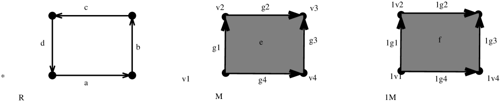
$x_{P}=v_{1}$$t_{1}$$v_{2}$$t_{2}$$v_{3}$$t_{3}$$v_{4}$$t_{4}$${\bf P}$$\partial_{L}^{Q}(P)\;=t_{4}t_{3}t_{2}^{-1}t_{1}^{-1}$$\gamma_{1}$$\gamma_{2}$$\gamma_{3}$$\gamma_{4}$$g_{t_{1}}$$g_{t_{2}}$$g_{t_{3}}$$g_{t_{4}}$${\bf e_{P}}$$\partial_{{\cal G}}(e_{P})\;=g_{t_{4}}g_{t_{3}}g_{t_{2}}^{-1}g_{t_{1}}^{-1}$${Z_{P}},\textrm{ the CW-decomposition of }S^{1}$ $*=(0,0)$

Figure 4: A 2-lattice decomposition $L$ of $D^{2}$, where ${Z_{P}}$ is the corresponding CW-decomposition of $S^{1}$: cf. Def, 21. The base-point $x_{P}$ of $P$ is $v_{1}$. We also show a fake-flat 2-gauge configuration in $(D^{2},L)$.

For this example, the quantised boundary of the plaquette $P$ is $\partial_{L}^{Q}(P)\;=t_{4}t_{3}t_{2}^{-1}t_{1}^{-1}.$ Hence a 2-gauge configuration of $([0,1]^{2},L)$ is given by four elements $g_{t_{1}},g_{t_{2}},g_{t_{3}},g_{t_{4}}$ of $G$, the colours of the edges, $t_{1}$, $t_{2}$, $t_{3}$, $t_{4}$, and an element $e_{P}\in E$, colouring $P$. The fake flateness conditions says: $\partial_{{\cal G}}(e_{P})=g_{t_{4}}g_{t_{3}}g_{t_{2}}^{-1}g_{t_{1}}^{-1}.$

Let $\Theta(M,L,{\cal G})$ denote the set of fake-flat 2-gauge configurations. Note that $\Theta(M,L,{\cal G})$ is non-empty. In particular the ‘naive vacuum’ $\Omega_{1}$ given by $e_{P}=1_{E}$ for all plaquettes $P$ of $(M,L)$ and $g_{t}=1_{G}$ for all edges $t$ is fake-flat. Here $1_{G}$ and $1_{E}$ denote the identities of $G$ and $E$.

3.3 On Whitehead theorem, 2-gauge configurations and the lattice 2-groupoid

Let $(M,L)$ be a 2-lattice. Passing to the 0, 1 and 2-skeletons of the corresponding CW-decomposition of $M$, yields a triple $(M^{2},M^{1},M^{0})$ of locally path-connected spaces, where $M^{0}$ intersects non-trivially any path-connected component of $M^{1}$ and $M^{2}$. Utilising Def. 10, we can form the fundamental crossed module $\Pi_{2}(M^{2},M^{1},M^{0})$; Thm. 11. This crossed module plays the role of lattice 2-groupoid of $(M,L)$.

Observe that to make use of our fake-flat 2-gauge configurations we need corresponding lifts of Lem. 36 and Thm. 38. Analogously to Thm. 38, the crossed module $\Pi_{2}(M^{2},M^{1},M^{0})$ is free on the attaching maps of the geometric plaquettes (i.e. closed 2-cells) of $(M,L)$. This result (which holds in the general case of CW-complexes) is an old result due to JHC Whitehead [70]. Modern treatments can be found in [18, 11, 10, 13, 8].

Consider groupoids $H=(\sigma,\tau\colon H_{1}\to H_{0})$ and $H^{\prime}=(\sigma,\tau\colon H_{1}^{\prime}\to H_{0}^{\prime})$. Throughout this subsection, we use the following notation. If $f\colon H\to H^{\prime}$ is a groupoid map, put $f_{\rm MOR}\colon H_{1}\to H_{1}^{\prime}$ to be the restriction of $f$ to morphisms and $f_{\rm OBJ}\colon H_{0}\to H^{\prime}_{0}$ to be the restriction of $f$ to objects. If $(\partial\colon E\to G)$ is a a crossed module of groupoids, thus $E$ and $G$ have the same set $C$ of objects, it holds that $\partial_{\rm OBJ}\colon C\to C$ is the identity map.

In order not to excessively load our formulae, we use the same notation for the groupoid $\pi_{2}(M^{2},M^{1},M^{0})$ and for its set of morphisms, and the same for $\pi_{1}(M^{1},M^{0})$. Which one is meant is clear from the context. The coinciding source and target maps in the groupoid $\pi_{2}(M^{2},M^{1},M^{0})$ are given by the obvious map:

$${\beta\colon\pi_{2}(M^{2},M^{1},M^{0})\doteq\bigsqcup_{v\in M^{0}}\pi_{2}(M^{2},M^{1},v)\to M^{0}.}$$

First we specify what “crossed module freeness” is. Let $G=(\sigma,\tau\colon G_{1}\to G_{0})$ be a groupoid. Let also $K$ be a set mapping to $G_{0}$, through a map $\beta_{0}$. Suppose also that we have a map $\partial_{0}\colon K\to G_{1}$ that makes the diagram below commute (therefore $\beta_{0}=\tau\circ\partial_{0}$ and $\beta_{0}=\sigma\circ\partial_{0})$:

(6)

(This in particular means that $\partial_{0}$ is a map from $K$ into the set of arrows (morphisms) in $G$ that have the same source and target.) Let $F=(\beta,\beta\colon F_{1}\to G_{0})$ be a totally intransitive groupoid with the same set of objects as $G$. We say that a crossed module of groupoids $(\partial\colon F\to G,\triangleright)$ is free on $\partial_{0}\colon K\to G_{1}$ (or more precisely on $\partial_{0}\colon K\to G_{1}$ and $\beta_{0}\colon K\to G_{0}$ as in (6)) if there exists an inclusion (set) map ${\rm inc}\colon K\to F_{1}$ making the diagram below commute:

(7)

such that the following universal property is satisfied: Given any crossed module $(\partial^{\prime}\colon E^{\prime}\to G^{\prime},\triangleright)$ of groupoids, where $G^{\prime}=(\sigma^{\prime},\tau^{\prime}\colon G_{1}^{\prime}\to G_{0}^{\prime})$ and $E^{\prime}=(\beta^{\prime},\beta^{\prime}\colon E_{1}^{\prime}\to G_{0}^{\prime})$, and any groupoid map $\phi\colon G\to G^{\prime}$, and any set map $\psi_{0}\colon K\to E^{\prime}_{1}$, such that $\partial^{\prime}_{\rm MOR}\circ\psi_{0}=\phi_{\rm MOR}\circ\partial_{0}$, there exists a unique groupoid map $\psi\colon F\to E^{\prime}$, with $\psi_{\rm OBJ}=\phi_{\rm OBJ}$, making the diagram below commutative:

(8)

and so that the pair $(\psi,\phi)$ of groupoid maps is a crossed module map $(\partial\colon F\to G)\to(\partial^{\prime}\colon E^{\prime}\to G^{\prime})$.

Lemma 50.

Given $\partial_{0}\colon K\to G_{1}$ as in (6), the totally intransitive groupoid $F=(\beta,\beta\colon F_{1}\to G_{0})$, i.e. the top groupoid of the free crossed module on $\partial_{0}\colon K\to G_{1}$, is uniquely specified up to isomorphism by the universal property above. A model for $F$ is the following. First of all note that we have a totally intransitive graph $K^{\prime}$ having $G_{0}$ as set of vertices and the set of edges being the set of all pairs $(g,k)$, where $g\in G_{1}$ and $k\in K$ are such that $\tau(g)=\beta_{0}(k)$. The coinciding source and target maps of $K^{\prime}$ are given by $(g,k)\mapsto\sigma(g)$. Edges of $K^{\prime}$ therefore take the form:

$$\sigma(g)\xrightarrow{(g,k)}\sigma(g),\textrm{ where }g\in G_{1}\textrm{ and }k\in K\textrm{ are such that }\tau(g)=\beta_{0}(k).$$

We then form the free groupoid $FG(K^{\prime})$, which is a totally intransitive groupoid having $G_{0}$ as set of objects. We have a groupoid map $\partial\colon FG(K^{\prime})\to G$ which is the identity on objects and on generating morphisms is:

$${\partial_{\rm MOR}\big{(}\sigma(g)\xrightarrow{(g,k)}\sigma(g)\big{)}\;=\;\sigma(g)\xrightarrow{g\partial_{0}(k)g^{-1}}\sigma(g).}$$

The groupoid $FG(K^{\prime})$ has a natural left action by automorphisms of the groupoid $G$. On generators of $FG(K^{\prime})$, the action takes the following form: If $g,h\in{G_{1}}$ are such that $\tau(h)=\sigma(g)$, and $k\in K$ is such that $\beta_{0}(k)=\tau(g)$, put $h.(g,k)=(hg,k)$. Then together with the map $\partial\colon FG(K^{\prime})\to G$, nearly all conditions that crossed modules of groupoids must satisfy (Def. 2 and 6) hold, except for the 2nd Peiffer relation. The groupoid $F$ is obtained from $FG(K^{\prime})$ by dividing out the 2nd Peiffer relations, in the obvious way.

Proof.

Routine. Details are in [18, §7.3(ii)] and [11]. ∎

Let $(M,L)$ be a 2-lattice. Recall Rem. 29 and 30, and Def. 21. Going back to $\Pi_{2}(M^{2},M^{1},M^{0})$, to each plaquette $P\in L^{2}$ we can associate elements $\partial_{L}(P)\in\pi_{1}(M^{1},x_{P})\subset\pi_{1}(M^{1},M^{0})$ and $\iota_{L}(P)\in\pi_{2}(M^{2},M^{1},x_{P})$, where $x_{P}=\psi_{P}^{2}(*)$ is the base-point of the closed 2-cell $\overline{c_{P}^{2}}$ corresponding to $P$. Also $\partial_{\rm MOR}(\iota_{L}(P))=\partial_{L}(P)$. In particular we have a commutative diagram as in (6,7,8):

Hence we can form the free crossed module $(\partial\colon F\to\pi_{1}(M^{1},M^{0}),\triangleright)$ on $\partial_{L}\colon L^{2}\to\pi_{1}(M^{1},M^{0})$, where $F=(\beta,\beta\colon F_{1}\to M^{0})$. And we have a unique groupoid morphism $\iota\colon F\to\pi_{2}(M^{2},M^{1},M^{0})$, which is the identity on objects, that makes the diagram below commutative, and so that $(\iota,{\mathrm{id}})\colon(F\to\pi_{1}(M^{1},M^{0}),\triangleright)\to\Pi_{2}(M^{2},M^{1},M^{0})$ is a crossed module map:

(9)

Theorem 51 (Whitehead Theorem).

Let $(M,L)$ be a 2-lattice, or indeed any CW-complex. Then the crossed module $\Pi_{2}(M^{2},M^{1},M^{0})=(\partial\colon\pi_{2}(M^{2},M^{1},M^{0})\rightarrow\pi_{1}(M^{1},M^{0}),\triangleright)$ is free on $\partial_{L}\colon L^{2}\to\pi_{1}(M^{1},M^{0})$. Specifically, the map $\iota\colon F\to\pi_{2}(M^{2},M^{1},M^{0})$ defined from (9) is an isomorphism of groupoids, and, moreover, the pair $(\iota,{\mathrm{id}})\colon(\partial\colon F\to\pi_{1}(M^{1},M^{0}),\triangleright)\to\Pi_{2}(M^{2},M^{1},M^{0})$ is an isomorphism of crossed modules.

Proof.

See [18, §6] and [13, 11, 14, 15], where Whitehead’s theorem is deduced from the more general 2-dimensional van Kampen theorem, and also [10, 8]. (We note that Whitehead’s original proof was done for crossed modules of groups rather than of groupoids, and only considered spaces with a single base-point.)∎

Remark 52.

Note that Whitehead’s theorem together with the construction of free crossed modules (Lem. 50) implies that the totally intransitive groupoid $\pi_{2}(M^{2},M^{1},M^{0})$ is generated by $\sigma(g)\xrightarrow{g\triangleright\iota_{L}(P)}\sigma(g)$, where $g\in\pi_{1}(M^{1},M^{0})$ and $P\in L^{2}$ is such that: $x_{P}=\tau(g)$; recall that $\sigma(g)$ and $\tau(g)$ are the initial and end-points of $g$ and $x_{P}$ is the base-point of $P$. This will have a primary role in the construction of the 2-dimensional holonomy of a fake-flat 2-gauge configuration along a cellularly embebbed surface in §3.4.

We will only use the universal property (8) in the case when ${\cal G}=(\partial^{\prime}\colon E^{\prime}\to G^{\prime},\triangleright)$ is a crossed module of groups. In this case there is not much to worry about maps on object sets of groupoids, as $E^{\prime}$ and $G^{\prime}$ are groupoids with a single object. We hence will not display the related part of the commutative diagrams. Given groupoid maps $f\colon\pi_{1}(M^{1},M^{0})\to G^{\prime}$ and $f^{\prime}\colon\pi_{2}(M^{2},M^{1},M^{0})\to E^{\prime}$ we put $f_{\rm MOR}=f$ and $f^{\prime}_{\rm MOR}=f^{\prime}$. In ${\cal G}$, we put $\partial^{\prime}_{\rm MOR}=\partial^{\prime}$. Recall that we use the same notation for the groupoid $\pi_{2}(M^{2},M^{1},M^{0})$ and for its set of morphisms, and the same for $\pi_{1}(M^{1},M^{0})$.

Whitehead’s theorem implies the following. Consider the inclusion map $\iota_{L}\colon L^{2}\to\pi_{2}(M^{2},M^{1},M^{0})$, with $\partial_{\rm MOR}\circ{\iota_{L}}=\partial_{L}$, cf. Rem. 29 and 30. If $G^{\prime}$ is a group, $(\partial^{\prime}\colon E^{\prime}\to G^{\prime},\triangleright)$ is a crossed module of groups, and $\phi\colon\pi_{1}(M^{1},M^{0})\to G^{\prime}$ is a groupoid map, then given any set map $\psi_{0}\colon L^{2}\to E^{\prime}$ such that $\phi\circ\partial_{L}=\partial^{\prime}\circ\psi_{0}$, there exists a unique groupoid map $\psi\colon\pi_{2}(M^{2},M^{1},M^{0})\to E^{\prime}$ making the diagram below commutative and also making the pair $(\psi,\phi)$ a crossed module map $\Pi_{2}(M^{2},M^{1},M^{0})\to{\cal G}$ (thus $(\psi,\phi)$ is compatible with boundaries and groupoid actions):

$${\lx@xy@svg{\hbox{\raise 0.0pt\hbox{\kern 3.0pt\hbox{\ignorespaces\ignorespaces\ignorespaces\hbox{\vtop{\kern 0.0pt\offinterlineskip\halign{\entry@#!@&&\entry@@#!@\cr&&&\\&&&\crcr}}}\ignorespaces{\hbox{\kern-3.0pt\raise 0.0pt\hbox{\hbox{\kern 0.0pt\raise 0.0pt\hbox{\hbox{\kern 3.0pt\raise 0.0pt\hbox{$\textstyle{}$}}}}}}}{\hbox{\kern 27.0pt\raise 0.0pt\hbox{\hbox{\kern 0.0pt\raise 0.0pt\hbox{\hbox{\kern 3.0pt\raise 0.0pt\hbox{$\textstyle{L^{2}\ignorespaces\ignorespaces\ignorespaces\ignorespaces\ignorespaces\ignorespaces\ignorespaces\ignorespaces\ignorespaces\ignorespaces\ignorespaces\ignorespaces\ignorespaces\ignorespaces}$}}}}}}}\ignorespaces\ignorespaces\ignorespaces\ignorespaces\ignorespaces{}{}{}{{}{}{}{}{}{}{}{}{}{}{}{}{}{}{}}{}\ignorespaces\hbox{\hbox{\kern 0.0pt\raise 0.0pt\hbox{{}{}{{}}{{}{}{}}{}}}}\ignorespaces{}\ignorespaces{}{}{}{{}{}}\ignorespaces\ignorespaces{\hbox{\kern 96.26982pt\raise 18.1111pt\hbox{{}\hbox{\kern 0.0pt\raise 0.0pt\hbox{\hbox{\kern 3.0pt\hbox{\hbox{\kern 0.0pt\raise-1.75pt\hbox{$\scriptstyle{\psi_{0}}$}}}\kern 3.0pt}}}}}}\ignorespaces{}{}{}{{}{}{}{}{}{}{}{}{}{}{}{}{}{}{}{}{}{}}{\hbox{\kern 162.556pt\raise 2.58554pt\hbox{\hbox{\kern 0.0pt\raise 0.0pt\hbox{\lx@xy@tip{1}\lx@xy@tip{-1}}}}}}\ignorespaces\hbox{\hbox{\kern 0.0pt\raise 0.0pt\hbox{{}{}{}{{}}{{}{}{}\lx@xy@spline@}{}}}}\ignorespaces{}\ignorespaces\hbox{\hbox{\kern 0.0pt\raise 0.0pt\hbox{{}{}{{}}{{}{}{}}{}}}}\ignorespaces{}\ignorespaces\ignorespaces\ignorespaces{}\ignorespaces\ignorespaces{\hbox{\lx@xy@drawline@}}\ignorespaces\ignorespaces\ignorespaces{\hbox{\kern 58.69264pt\raise-26.68275pt\hbox{{}\hbox{\kern 0.0pt\raise 0.0pt\hbox{\hbox{\kern 3.0pt\hbox{\hbox{\kern 0.0pt\raise-1.74722pt\hbox{$\scriptstyle{\partial_{L}}$}}}\kern 3.0pt}}}}}}\ignorespaces{\hbox{\kern 83.41512pt\raise-29.5pt\hbox{\hbox{\kern 0.0pt\raise 0.0pt\hbox{\lx@xy@tip{1}\lx@xy@tip{-1}}}}}}\ignorespaces\ignorespaces{\hbox{\lx@xy@drawline@}}\ignorespaces{\hbox{\lx@xy@drawline@}}\ignorespaces\ignorespaces\ignorespaces\ignorespaces{}{\hbox{\lx@xy@droprule}}\ignorespaces{\hbox{\kern 52.00568pt\raise 0.0pt\hbox{\hbox{\kern 0.0pt\raise-0.82361pt\hbox{$\scriptstyle{\iota_{L}}$}}}}}{\hbox{\lx@xy@droprule}}\ignorespaces{\hbox{\kern 66.60556pt\raise 0.0pt\hbox{\hbox{\kern 0.0pt\raise 0.0pt\hbox{\lx@xy@tip{1}\lx@xy@tip{-1}}}}}}{\hbox{\lx@xy@droprule}}{\hbox{\lx@xy@droprule}}{\hbox{\kern 66.60556pt\raise 0.0pt\hbox{\hbox{\kern 0.0pt\raise 0.0pt\hbox{\hbox{\kern 3.0pt\raise 0.0pt\hbox{$\textstyle{\pi_{2}(M^{2},M^{1},M^{0})\ignorespaces\ignorespaces\ignorespaces\ignorespaces\ignorespaces\ignorespaces\ignorespaces\ignorespaces}$}}}}}}}\ignorespaces\ignorespaces\ignorespaces\ignorespaces{}{\hbox{\lx@xy@droprule}}\ignorespaces\ignorespaces\ignorespaces{\hbox{\kern 102.57649pt\raise-20.56888pt\hbox{{}\hbox{\kern 0.0pt\raise 0.0pt\hbox{\hbox{\kern 3.0pt\hbox{\hbox{\kern 0.0pt\raise-1.74722pt\hbox{$\scriptstyle{\partial_{\rm MOR}}$}}}\kern 3.0pt}}}}}}\ignorespaces{\hbox{\kern 102.57649pt\raise-29.5pt\hbox{\hbox{\kern 0.0pt\raise 0.0pt\hbox{\lx@xy@tip{1}\lx@xy@tip{-1}}}}}}{\hbox{\lx@xy@droprule}}{\hbox{\lx@xy@droprule}}\ignorespaces\ignorespaces\ignorespaces{}\ignorespaces\ignorespaces{\hbox{\lx@xy@drawline@}}\ignorespaces\ignorespaces\ignorespaces{\hbox{\kern 145.26756pt\raise-6.1111pt\hbox{{}\hbox{\kern 0.0pt\raise 0.0pt\hbox{\hbox{\kern 3.0pt\hbox{\hbox{\kern 0.0pt\raise-1.75pt\hbox{$\scriptstyle{\psi}$}}}\kern 3.0pt}}}}}}\ignorespaces{\hbox{\kern 162.54742pt\raise 0.0pt\hbox{\hbox{\kern 0.0pt\raise 0.0pt\hbox{\lx@xy@tip{1}\lx@xy@tip{-1}}}}}}\ignorespaces\ignorespaces{\hbox{\lx@xy@drawline@}}\ignorespaces{\hbox{\lx@xy@drawline@}}{\hbox{\kern 162.54742pt\raise 0.0pt\hbox{\hbox{\kern 0.0pt\raise 0.0pt\hbox{\hbox{\kern 3.0pt\raise 0.0pt\hbox{$\textstyle{E^{\prime}\ignorespaces\ignorespaces\ignorespaces\ignorespaces}$}}}}}}}\ignorespaces\ignorespaces\ignorespaces\ignorespaces{}{\hbox{\lx@xy@droprule}}\ignorespaces\ignorespaces\ignorespaces{\hbox{\kern 159.48026pt\raise-20.56888pt\hbox{{}\hbox{\kern 0.0pt\raise 0.0pt\hbox{\hbox{\kern 3.0pt\hbox{\hbox{\kern 0.0pt\raise-2.98611pt\hbox{$\scriptstyle{\partial^{\prime}}$}}}\kern 3.0pt}}}}}}\ignorespaces{\hbox{\kern 170.29657pt\raise-29.74889pt\hbox{\hbox{\kern 0.0pt\raise 0.0pt\hbox{\lx@xy@tip{1}\lx@xy@tip{-1}}}}}}{\hbox{\lx@xy@droprule}}{\hbox{\lx@xy@droprule}}{\hbox{\kern-3.0pt\raise-41.13776pt\hbox{\hbox{\kern 0.0pt\raise 0.0pt\hbox{\hbox{\kern 3.0pt\raise 0.0pt\hbox{$\textstyle{}$}}}}}}}{\hbox{\kern 31.80278pt\raise-41.13776pt\hbox{\hbox{\kern 0.0pt\raise 0.0pt\hbox{\hbox{\kern 3.0pt\raise 0.0pt\hbox{$\textstyle{}$}}}}}}}{\hbox{\kern 75.6236pt\raise-41.13776pt\hbox{\hbox{\kern 0.0pt\raise 0.0pt\hbox{\hbox{\kern 3.0pt\raise 0.0pt\hbox{$\textstyle{\pi_{1}(M^{1},M^{0})\ignorespaces\ignorespaces\ignorespaces\ignorespaces}$}}}}}}}\ignorespaces\ignorespaces\ignorespaces\ignorespaces{}{\hbox{\lx@xy@droprule}}\ignorespaces\ignorespaces\ignorespaces{\hbox{\kern 145.50992pt\raise-35.02666pt\hbox{{}\hbox{\kern 0.0pt\raise 0.0pt\hbox{\hbox{\kern 3.0pt\hbox{\hbox{\kern 0.0pt\raise-1.75pt\hbox{$\scriptstyle{\phi}$}}}\kern 3.0pt}}}}}}\ignorespaces{\hbox{\kern 162.59534pt\raise-41.13776pt\hbox{\hbox{\kern 0.0pt\raise 0.0pt\hbox{\lx@xy@tip{1}\lx@xy@tip{-1}}}}}}{\hbox{\lx@xy@droprule}}{\hbox{\lx@xy@droprule}}{\hbox{\kern 162.59534pt\raise-41.13776pt\hbox{\hbox{\kern 0.0pt\raise 0.0pt\hbox{\hbox{\kern 3.0pt\raise 0.0pt\hbox{$\textstyle{G^{\prime}}$}}}}}}}\ignorespaces}}}}\ignorespaces}. \textstyle{L^{2}\ignorespaces\ignorespaces\ignorespaces\ignorespaces\ignorespaces\ignorespaces\ignorespaces\ignorespaces\ignorespaces\ignorespaces\ignorespaces\ignorespaces\ignorespaces\ignorespaces} \scriptstyle{\psi_{0}} \scriptstyle{\partial_{L}} \scriptstyle{\iota_{L}} \textstyle{\pi_{2}(M^{2},M^{1},M^{0})\ignorespaces\ignorespaces\ignorespaces\ignorespaces\ignorespaces\ignorespaces\ignorespaces\ignorespaces} \scriptstyle{\partial_{\rm MOR}} \scriptstyle{\psi} \textstyle{E^{\prime}\ignorespaces\ignorespaces\ignorespaces\ignorespaces} \scriptstyle{\partial^{\prime}} \textstyle{\pi_{1}(M^{1},M^{0})\ignorespaces\ignorespaces\ignorespaces\ignorespaces} \scriptstyle{\phi} \textstyle{G^{\prime}} \textstyle{L^{2}\ignorespaces\ignorespaces\ignorespaces\ignorespaces\ignorespaces\ignorespaces\ignorespaces\ignorespaces\ignorespaces\ignorespaces\ignorespaces\ignorespaces\ignorespaces\ignorespaces} \scriptstyle{\psi_{0}} \scriptstyle{\partial_{L}} \scriptstyle{\iota_{L}} \textstyle{\pi_{2}(M^{2},M^{1},M^{0})\ignorespaces\ignorespaces\ignorespaces\ignorespaces\ignorespaces\ignorespaces\ignorespaces\ignorespaces} \scriptstyle{\partial_{\rm MOR}} \scriptstyle{\psi} \textstyle{E^{\prime}\ignorespaces\ignorespaces\ignorespaces\ignorespaces} \scriptstyle{\partial^{\prime}} \textstyle{\pi_{1}(M^{1},M^{0})\ignorespaces\ignorespaces\ignorespaces\ignorespaces} \scriptstyle{\phi} \textstyle{G^{\prime}}$$ (10)

3.3.1 The discrete 2-dimensional (2D) parallel transport of a fake-flat 2-gauge configuration

As promised in 3.1, we now state and prove the analogue of Thm. 40 for fake-flat 2-gauge configurations.

Let $(M,L)$ be a 2-lattice and ${\cal G}=(\partial_{{\cal G}}\colon E\to G,\triangleright)$ be a group crossed module.

Theorem 53 (The discrete 2D parallel transport of a fake-flat 2-gauge configuration).

There exists a one-to-one correspondence between fake-flat 2-gauge configurations ${\cal F}=({\cal F}^{2},{\cal F}^{1})$ in $(M,L)$ and crossed module maps $(\Psi_{\cal F},\Phi_{\cal F})\colon\Pi_{2}(M^{2},M^{1},M^{0})\to{\cal G}.$ (Note $\Psi_{\cal F}\colon\pi_{2}(M^{2},M^{1},M^{0})\to E$ and $\Phi_{\cal F}\colon\pi_{1}(M^{1},M^{0})\to G$ therefore are groupoid maps, compatible with boundary maps and groupoid actions in the obvious way.)

In analogy with the differential-geometric construction of 2-dimensional parallel transport 2-functors attached to 2-connections on 2-bundles [61, 32], the crossed module map $(\Psi_{\cal F},\Phi_{\cal F})\colon\Pi_{2}(M^{2},M^{1},M^{0})\to{\cal G}$ associated to a fake-flat 2-gauge configurations ${\cal F}$ will be called the discrete 2D parallel transport 2-functor of ${\cal F}$.

Proof.

Recall the notation introduced after Thm 51. A fake-flat 2-gauge configuration ${\cal F}=({\cal F}^{2}\colon L^{2}\to E\,\,,\,\,{\cal F}^{1}\colon L^{1}\to G)$ is an assignment $\gamma\mapsto g_{\gamma}$ of an element of $G$ to each 1-cell $\gamma$ of $L$, and an assigment $P\mapsto e_{P}$ of an element of $E$ to each 2-cell $P$, satisfying the fake-flatness condition of Def. 46. Whitehead’s theorem (Thm 51) states that the fundamental crossed module $\Pi_{2}(M,M^{1},M^{0})$, with set $M^{0}$ of base points – a crossed module of groupoids, is isomorphic to the free crossed module on the map $\partial_{L}\colon L^{2}\to\pi_{1}(M^{1},M^{0})$.

Since the groupoid $\pi_{1}(M^{1},M^{0})$ is free on the 1-cells, the assignment ${\cal F}^{1}\colon\gamma\in L^{1}\mapsto g_{\gamma}\in G$ uniquely extends to a groupoid map $\Phi_{\cal F}=\Phi_{{\cal F}^{1}}\colon{\pi_{1}(M^{1},M^{0})}\to G$. The fake-flatness condition means that the outer part of the diagram below commutes:

$${\lx@xy@svg{\hbox{\raise 0.0pt\hbox{\kern 3.0pt\hbox{\ignorespaces\ignorespaces\ignorespaces\hbox{\vtop{\kern 0.0pt\offinterlineskip\halign{\entry@#!@&&\entry@@#!@\cr&&&\\&&&\crcr}}}\ignorespaces{\hbox{\kern-3.0pt\raise 0.0pt\hbox{\hbox{\kern 0.0pt\raise 0.0pt\hbox{\hbox{\kern 3.0pt\raise 0.0pt\hbox{$\textstyle{}$}}}}}}}{\hbox{\kern 27.0pt\raise 0.0pt\hbox{\hbox{\kern 0.0pt\raise 0.0pt\hbox{\hbox{\kern 3.0pt\raise 0.0pt\hbox{$\textstyle{L^{2}\ignorespaces\ignorespaces\ignorespaces\ignorespaces\ignorespaces\ignorespaces\ignorespaces\ignorespaces\ignorespaces\ignorespaces\ignorespaces\ignorespaces\ignorespaces\ignorespaces}$}}}}}}}\ignorespaces\ignorespaces\ignorespaces\ignorespaces\ignorespaces{}{}{}{{}{}{}{}{}{}{}{}{}{}{}{}{}{}{}{}{}{}}{}\ignorespaces\hbox{\hbox{\kern 0.0pt\raise 0.0pt\hbox{{}{}{{}}{{}{}{}}{}}}}\ignorespaces{}\ignorespaces{}{}{}{{}{}}\ignorespaces\ignorespaces{\hbox{\kern 95.87996pt\raise 18.0361pt\hbox{{}\hbox{\kern 0.0pt\raise 0.0pt\hbox{\hbox{\kern 3.0pt\hbox{\hbox{\kern 0.0pt\raise-3.0361pt\hbox{$\scriptstyle{{\cal F}^{2}}$}}}\kern 3.0pt}}}}}}\ignorespaces{}{}{}{{}{}{}{}{}{}{}{}{}{}{}{}{}{}{}{}{}}{\hbox{\kern 162.55362pt\raise 2.35579pt\hbox{\hbox{\kern 0.0pt\raise 0.0pt\hbox{\lx@xy@tip{1}\lx@xy@tip{-1}}}}}}\ignorespaces\hbox{\hbox{\kern 0.0pt\raise 0.0pt\hbox{{}{}{}{{}}{{}{}{}\lx@xy@spline@}{}}}}\ignorespaces{}\ignorespaces\hbox{\hbox{\kern 0.0pt\raise 0.0pt\hbox{{}{}{{}}{{}{}{}}{}}}}\ignorespaces{}\ignorespaces\ignorespaces\ignorespaces{}\ignorespaces\ignorespaces{\hbox{\lx@xy@drawline@}}\ignorespaces\ignorespaces\ignorespaces{\hbox{\kern 58.69264pt\raise-26.68275pt\hbox{{}\hbox{\kern 0.0pt\raise 0.0pt\hbox{\hbox{\kern 3.0pt\hbox{\hbox{\kern 0.0pt\raise-1.74722pt\hbox{$\scriptstyle{\partial_{L}}$}}}\kern 3.0pt}}}}}}\ignorespaces{\hbox{\kern 83.41512pt\raise-29.5pt\hbox{\hbox{\kern 0.0pt\raise 0.0pt\hbox{\lx@xy@tip{1}\lx@xy@tip{-1}}}}}}\ignorespaces\ignorespaces{\hbox{\lx@xy@drawline@}}\ignorespaces{\hbox{\lx@xy@drawline@}}\ignorespaces\ignorespaces\ignorespaces\ignorespaces{}{\hbox{\lx@xy@droprule}}\ignorespaces{\hbox{\kern 49.00569pt\raise 0.0pt\hbox{\hbox{\kern 0.0pt\raise-0.82361pt\hbox{$\scriptstyle{\iota_{L}}$}}}}}{\hbox{\lx@xy@droprule}}\ignorespaces{\hbox{\kern 66.60556pt\raise 0.0pt\hbox{\hbox{\kern 0.0pt\raise 0.0pt\hbox{\lx@xy@tip{1}\lx@xy@tip{-1}}}}}}{\hbox{\lx@xy@droprule}}{\hbox{\lx@xy@droprule}}{\hbox{\kern 66.60556pt\raise 0.0pt\hbox{\hbox{\kern 0.0pt\raise 0.0pt\hbox{\hbox{\kern 3.0pt\raise 0.0pt\hbox{$\textstyle{\pi_{2}(M^{2},M^{1},M^{0})\ignorespaces\ignorespaces\ignorespaces\ignorespaces\ignorespaces\ignorespaces\ignorespaces\ignorespaces}$}}}}}}}\ignorespaces\ignorespaces\ignorespaces\ignorespaces{}{\hbox{\lx@xy@droprule}}\ignorespaces\ignorespaces\ignorespaces{\hbox{\kern 102.57649pt\raise-20.56888pt\hbox{{}\hbox{\kern 0.0pt\raise 0.0pt\hbox{\hbox{\kern 3.0pt\hbox{\hbox{\kern 0.0pt\raise-1.74722pt\hbox{$\scriptstyle{\partial_{\rm MOR}}$}}}\kern 3.0pt}}}}}}\ignorespaces{\hbox{\kern 102.57649pt\raise-29.5pt\hbox{\hbox{\kern 0.0pt\raise 0.0pt\hbox{\lx@xy@tip{1}\lx@xy@tip{-1}}}}}}{\hbox{\lx@xy@droprule}}{\hbox{\lx@xy@droprule}}\ignorespaces\ignorespaces\ignorespaces{}\ignorespaces\ignorespaces{\hbox{\lx@xy@drawline@}}\ignorespaces\ignorespaces\ignorespaces{\hbox{\kern 140.51964pt\raise-6.075pt\hbox{{}\hbox{\kern 0.0pt\raise 0.0pt\hbox{\hbox{\kern 3.0pt\hbox{\hbox{\kern 0.0pt\raise-1.70833pt\hbox{$\scriptstyle{\Psi_{\cal F}}$}}}\kern 3.0pt}}}}}}\ignorespaces{\hbox{\kern 162.54742pt\raise 0.0pt\hbox{\hbox{\kern 0.0pt\raise 0.0pt\hbox{\lx@xy@tip{1}\lx@xy@tip{-1}}}}}}\ignorespaces\ignorespaces{\hbox{\lx@xy@drawline@}}\ignorespaces{\hbox{\lx@xy@drawline@}}{\hbox{\kern 162.54742pt\raise 0.0pt\hbox{\hbox{\kern 0.0pt\raise 0.0pt\hbox{\hbox{\kern 3.0pt\raise 0.0pt\hbox{$\textstyle{E\ignorespaces\ignorespaces\ignorespaces\ignorespaces}$}}}}}}}\ignorespaces\ignorespaces\ignorespaces\ignorespaces{}{\hbox{\lx@xy@droprule}}\ignorespaces\ignorespaces\ignorespaces{\hbox{\kern 156.67137pt\raise-20.56888pt\hbox{{}\hbox{\kern 0.0pt\raise 0.0pt\hbox{\hbox{\kern 3.0pt\hbox{\hbox{\kern 0.0pt\raise-1.74722pt\hbox{$\scriptstyle{\partial_{{\cal G}}}$}}}\kern 3.0pt}}}}}}\ignorespaces{\hbox{\kern 169.52658pt\raise-31.30444pt\hbox{\hbox{\kern 0.0pt\raise 0.0pt\hbox{\lx@xy@tip{1}\lx@xy@tip{-1}}}}}}{\hbox{\lx@xy@droprule}}{\hbox{\lx@xy@droprule}}{\hbox{\kern-3.0pt\raise-41.13776pt\hbox{\hbox{\kern 0.0pt\raise 0.0pt\hbox{\hbox{\kern 3.0pt\raise 0.0pt\hbox{$\textstyle{}$}}}}}}}{\hbox{\kern 31.80278pt\raise-41.13776pt\hbox{\hbox{\kern 0.0pt\raise 0.0pt\hbox{\hbox{\kern 3.0pt\raise 0.0pt\hbox{$\textstyle{}$}}}}}}}{\hbox{\kern 75.6236pt\raise-41.13776pt\hbox{\hbox{\kern 0.0pt\raise 0.0pt\hbox{\hbox{\kern 3.0pt\raise 0.0pt\hbox{$\textstyle{\pi_{1}(M^{1},M^{0})\ignorespaces\ignorespaces\ignorespaces\ignorespaces}$}}}}}}}\ignorespaces\ignorespaces\ignorespaces\ignorespaces{}{\hbox{\lx@xy@droprule}}\ignorespaces\ignorespaces\ignorespaces{\hbox{\kern 143.76201pt\raise-35.06276pt\hbox{{}\hbox{\kern 0.0pt\raise 0.0pt\hbox{\hbox{\kern 3.0pt\hbox{\hbox{\kern 0.0pt\raise-1.70833pt\hbox{$\scriptstyle{\Phi_{\cal F}}$}}}\kern 3.0pt}}}}}}\ignorespaces{\hbox{\kern 162.59534pt\raise-41.13776pt\hbox{\hbox{\kern 0.0pt\raise 0.0pt\hbox{\lx@xy@tip{1}\lx@xy@tip{-1}}}}}}{\hbox{\lx@xy@droprule}}{\hbox{\lx@xy@droprule}}{\hbox{\kern 162.59534pt\raise-41.13776pt\hbox{\hbox{\kern 0.0pt\raise 0.0pt\hbox{\hbox{\kern 3.0pt\raise 0.0pt\hbox{$\textstyle{G}$}}}}}}}\ignorespaces}}}}\ignorespaces.} \textstyle{L^{2}\ignorespaces\ignorespaces\ignorespaces\ignorespaces\ignorespaces\ignorespaces\ignorespaces\ignorespaces\ignorespaces\ignorespaces\ignorespaces\ignorespaces\ignorespaces\ignorespaces} \scriptstyle{{\cal F}^{2}} \scriptstyle{\partial_{L}} \scriptstyle{\iota_{L}} \textstyle{\pi_{2}(M^{2},M^{1},M^{0})\ignorespaces\ignorespaces\ignorespaces\ignorespaces\ignorespaces\ignorespaces\ignorespaces\ignorespaces} \scriptstyle{\partial_{\rm MOR}} \scriptstyle{\Psi_{\cal F}} \textstyle{E\ignorespaces\ignorespaces\ignorespaces\ignorespaces} \scriptstyle{\partial_{{\cal G}}} \textstyle{\pi_{1}(M^{1},M^{0})\ignorespaces\ignorespaces\ignorespaces\ignorespaces} \scriptstyle{\Phi_{\cal F}} \textstyle{G} \textstyle{L^{2}\ignorespaces\ignorespaces\ignorespaces\ignorespaces\ignorespaces\ignorespaces\ignorespaces\ignorespaces\ignorespaces\ignorespaces\ignorespaces\ignorespaces\ignorespaces\ignorespaces} \scriptstyle{{\cal F}^{2}} \scriptstyle{\partial_{L}} \scriptstyle{\iota_{L}} \textstyle{\pi_{2}(M^{2},M^{1},M^{0})\ignorespaces\ignorespaces\ignorespaces\ignorespaces\ignorespaces\ignorespaces\ignorespaces\ignorespaces} \scriptstyle{\partial_{\rm MOR}} \scriptstyle{\Psi_{\cal F}} \textstyle{E\ignorespaces\ignorespaces\ignorespaces\ignorespaces} \scriptstyle{\partial_{{\cal G}}} \textstyle{\pi_{1}(M^{1},M^{0})\ignorespaces\ignorespaces\ignorespaces\ignorespaces} \scriptstyle{\Phi_{\cal F}} \textstyle{G}$$

And by applying the universal property defining free crossed modules of groupoids, in the particular form of (10), we can see that a gauge configuration ${\cal F}=({\cal F}^{2},{\cal F}^{1})$ can be extended (uniquely) to a crossed module map $(\Psi_{\cal F},\Phi_{\cal F})\colon\Pi_{2}(M,M^{1},M^{0})\to{{\cal G}}$, and all crossed module maps $\Pi_{2}(M,M^{1},M^{0})\to{{\cal G}}$ arise this way. ∎

Cf. 3.1. We have now explained the crossed module analogue of discrete parallel transport functors (Thm 40), in terms of discrete 2D parallel transport 2-functors. In the next two subsections §3.4 and §3.5, we address how the 2D parallel transport of a fake-flat 2-gauge configuration can be used to define notions of discrete 2D holonomy along surfaces $\Sigma$ cellularly embedded in a 2-lattice $(M,L)$. We will only deal with the case when $\Sigma$ is the 2-disk $D^{2}$ or the 2-sphere $S^{2}$. In these cases, which are the ones needed to define higher Kitaev models, a 2D holonomy can be associated to cellularly embedded surfaces $\Sigma\subset M$. 2D holonomy along 2-disks and 2-spheres is particularly simple to formulate, given that the corresponding oriented mapping class groups are trivial.

For surfaces $\Sigma$ not homeomorphic to $S^{2}$ or to $D^{2}$, additional information is needed to define a meaningful 2D holonomy for a cellular embedding of $\Sigma$ into $(M,L)$. Namely (assuming orientability) we must choose an isotopy class of homeomorphisms $\Sigma^{\prime}\to\Sigma$, where $\Sigma^{\prime}$ is the boundary of an unknotted handlebody in $\mathbb{R}^{3}$; see [32, 63]. We will address this more general 2D holonomy in a forthcoming publication.

3.4 Algebraic topological definition of 2D holonomy along 2-disks and 2-spheres

Let us fix a crossed module of groups ${\cal G}=(\partial_{{\cal G}}\colon E\to G,\triangleright)$. In this subsection we use elementary algebraic topology to define precisely and concisely the 2-dimensional (2D) holonomy of a fake-flat 2-gauge configuration along cellularly embedded 2-disks and 2-spheres; as such we present the 2D analogue of Rem. 43. A combinatorial definition of this 2D holonomy (therefore the analogue of Def. 42) will be dealt with in §3.5.

3.4.1 The 2-disk case

Let $(M,L)$ be a 2-lattice. Let $\Sigma$ be a surface embedded in $M$. Suppose that $\Sigma$ is homeomorphic to the 2-disk $D^{2}$. Suppose in addition that $\Sigma$ is oriented. Furthermore (cf. Def. 31) suppose that $L$ is a 2-lattice decomposition of the triple $(M,\Sigma,\mathrm{bd}(\Sigma))$, where $(\Sigma,\mathrm{bd}(\Sigma))$ is a pair homeomorphic to $(D^{2},S^{1})$. We have an induced relative CW-decomposition of $(\Sigma,\mathrm{bd}(\Sigma))$. Note $\Sigma=\Sigma^{2}$ (the 2-skeleton of $\Sigma$) and $\mathrm{bd}(\Sigma)\subset\Sigma^{1}.$

Choose a base point $v\in\mathrm{bd}(\Sigma)$. Since $\pi_{2}(\Sigma^{1},\mathrm{bd}(\Sigma),v)$ is trivial, the homotopy exact sequences of the triple $(\Sigma,\Sigma^{1},\mathrm{bd}(\Sigma))$ and of the pair $(\Sigma^{1},\mathrm{bd}(\Sigma))$ imply that the inclusion $(\Sigma,\mathrm{bd}(\Sigma))\to(\Sigma,\Sigma^{1})$ yields injections $\pi_{2}(\Sigma,\mathrm{bd}(\Sigma),v)\to\pi_{2}(\Sigma,\Sigma^{1},v)$ and $\pi_{1}(\mathrm{bd}(\Sigma),v)\to\pi_{1}(\Sigma^{1},v)$. We can thus see the crossed module $\Pi_{2}(\Sigma,\mathrm{bd}(\Sigma),v)\cong{({\mathrm{id}}\colon{\mathbb{Z}}\to{\mathbb{Z}})}$ (Ex. 13) as canonically included in $\Pi_{2}(\Sigma,\Sigma^{1},v)$.

Let $*=(0,0)$ be the common base point of $D^{2}$ and $S^{1}=\mathrm{bd}(D^{2})$. By elementary algebraic topology – since $\pi_{2}(D^{2},S^{1},*)={\mathbb{Z}}$ – any two pointed homeomorphisms $(D^{2},S^{1})\to(\Sigma,\mathrm{bd}(\Sigma))$ preserving orientation are homotopic as maps of pointed pairs $(D^{2},S^{1})\to(\Sigma,\mathrm{bd}(\Sigma))$. This is used in the definition below.

Definition 54 (Notation: $\partial_{v}(\Sigma,L)$ and $\iota_{v}(\Sigma,L)$).

Cf Rem. 29 and 30. Let $\Sigma$ be an oriented surface homeomorphic to $D^{2}$. Let $v\in\mathrm{bd}(\Sigma)$, the boundary of $\Sigma$. We will be mainly interested in the case when $v\in\mathrm{bd}(\Sigma)\cap M^{0}$. Consider a pointed orientation preserving homeomorphism $j\colon(D^{2},S^{1},*)\to(\Sigma,\mathrm{bd}(\Sigma),v)$. We let $j_{*}\colon\Pi_{2}(D^{2},S^{1},*)\to\Pi_{2}(\Sigma,\mathrm{bd}(\Sigma),v)$ be given by the induced map on homotopy groups. Let $\partial_{v}(\Sigma,v)\in\pi_{1}(\mathrm{bd}(\Sigma),v)\subset\pi_{1}(\Sigma^{1},v)$ be $\partial_{v}(\Sigma,v)=j_{*}(1),$ where $1$ is the positive (counterclockwise) generator of $\pi_{1}(S^{1},v)\cong{\mathbb{Z}}$. Hence $\partial_{v}(\Sigma,v)$ is a positively oriented loop along the boundary $\mathrm{bd}(\Sigma)$ of the 2-disk $\Sigma$, starting and ending at $v$. Analogously put $\iota_{v}(\Sigma,L)=j_{*}(1)\in\pi_{2}(\Sigma,\mathrm{bd}(\Sigma),v)\subset\pi_{2}(\Sigma,\Sigma^{1},v)$, where $1$ is now the positive generator of $\pi_{2}(D^{2},S^{1},v)\cong{\mathbb{Z}}$.

Note that by construction (cf. Ex 13):

$$\begin{split}\partial\big{(}\iota_{v}(\Sigma,L)\big{)}&=\partial_{v}(\Sigma,L),\\ \partial_{v}(\Sigma,L)\triangleright\iota_{v}(\Sigma,L)&=\iota_{v}(\Sigma,L).\end{split}$$ (11)

Lemma 55 (Dependence of $\partial_{v}(\Sigma,L)$ and $\iota_{v}(\Sigma,L)$ on $v\in\mathrm{bd}(\Sigma)$).

Suppose that $v\in M^{0}\cap\mathrm{bd}(\Sigma)$. Choose another $v^{\prime}\in M^{0}\cap\mathrm{bd}(\Sigma)$. Consider a path $\gamma$ in $\mathrm{bd}(\Sigma)$, connecting $v^{\prime}$ to $v$. (There are two different possible homotopy classes $[\gamma]$ for $\gamma$.) Then passing to the corresponding element $[\gamma]\in\pi_{1}(\Sigma^{1},\Sigma^{0})$, it holds that:

$${\begin{split}[\gamma]\triangleright\iota_{v}(\Sigma,L)&=\iota_{v^{\prime}}(\Sigma,L),\textrm{ in }\pi_{2}(\Sigma,\Sigma^{1},\Sigma^{0});\\ [\gamma]\,\partial_{v}(\Sigma,L)\,[\gamma]^{-1}&=\partial_{v^{\prime}}(\Sigma,L),\textrm{ in }\pi_{1}(\Sigma^{1},\Sigma^{0}).\end{split}}$$ (12)

Proof.

Follows from geometric considerations and the fact that $\pi_{1}(S^{1},*)$ acts trivially on $\pi_{2}(D^{2},S^{1},*)$. ∎

Let now ${\cal G}=(\partial_{{\cal G}}\colon E\to G,\triangleright)$ be a crossed module of groups.

Definition 56 (2D holonomy ${\rm Hol}_{v}({\cal F},\Sigma,L)$ of a fake-flat 2-gauge configuration ${\cal F}=({\cal F}^{2},{\cal F}^{1})$ along $\Sigma\cong D^{2}$, with initial point $v$).

Let $M$ be a topological manifold. Let $\Sigma$ be an oriented disk embedded in $M$. Let $L$ be a 2-lattice decomposition of $(M,\Sigma,\mathrm{bd}(\Sigma))$; see Def. 31. Let $v\in\mathrm{bd}(\Sigma)\cap M^{0}$. Let ${\cal F}$ be a fake-flat 2-gauge configuration in $(M,L)$, and ${\cal F}_{\Sigma}$ be its restriction to the induced 2-lattice decomposition of $\Sigma$. Let $(\Psi_{{\cal F}_{\Sigma}},\Phi_{{\cal F}_{\Sigma}})\colon\Pi_{2}(\Sigma,\Sigma^{1},\Sigma^{0})\to{\cal G}$ be the 2D parallel transport 2-functor of ${\cal F}_{\Sigma}$; Thm. 53. We define the 2D holonomy of ${\cal F}$ along $\Sigma$, with initial point $v$, as:

$${\rm Hol}_{v}({\cal F},\Sigma,L)=\left({\rm Hol}_{v}^{2}({\cal F},\Sigma,L),{\rm Hol}_{v}^{1}({\cal F},\Sigma,L)\right)=\Big{(}\Psi_{{\cal F}_{\Sigma}}(\iota_{v}(\Sigma,L)),\Phi_{{\cal F}_{\Sigma}}(\partial_{v}(\Sigma,L))\Big{)}\in E\times G.$$

In the conditions of Def. 56, note that:

$$\partial_{{\cal G}}\left({\rm Hol}_{v}^{2}({\cal F},\Sigma,L)\right)={\rm Hol}_{v}^{1}({\cal F},\Sigma,L).$$ (13)

This is because, by (11) and the fact that $(\Psi_{{\cal F}_{\Sigma}},\Phi_{{\cal F}_{\Sigma}})\colon\Pi_{2}(\Sigma,\Sigma^{1},\Sigma^{0})\to{\cal G}$ is a crossed module map:

$$\partial_{{\cal G}}\left({\rm Hol}_{v}^{2}({\cal F},\Sigma,L)\right) =\partial_{{\cal G}}(\Psi_{{\cal F}_{\Sigma}}(\iota_{v}(\Sigma,L))=\Phi_{{\cal F}_{\Sigma}}\big{(}\partial(\iota_{v}(\Sigma,L))\big{)}$$

$$=\Phi_{{\cal F}_{\Sigma}}(\partial_{v}(\Sigma,L))={\rm Hol}_{v}^{1}({\cal F},\Sigma,L).$$

Remark 57 (Dependence of 2D holonomy on base points).

The 2D holonomy ${\rm Hol}_{v}({\cal F},\Sigma,L)$ of a fake-flat 2-gauge configuration along a cellularly embedded 2-disk depends on the choice of a base point $v\in\mathrm{bd}(\Sigma)\cap M^{0}$. However, the dependence is mild. Cf. Rem. 55. Choose any quantised path $v^{\prime}\xrightarrow{\gamma}v$, in the boundary of the disk $\Sigma$, from the new base point $v^{\prime}$ to the initial base point $v$. Let $[\gamma]$ be the corresponding element of $\pi_{1}(\Sigma^{1},\Sigma^{0})\cong{\mathsf{FG}}\langle L^{0},L^{1}\rangle$. Then, since $(\Psi_{{\cal F}_{\Sigma}},\Phi_{{\cal F}_{\Sigma}})\colon\Pi_{2}(\Sigma,\Sigma^{1},\Sigma^{0})\to{\cal G}$ is a crossed module map:

$$\begin{split}{\rm{Hol}}_{v^{\prime}}^{2}({\cal F},\Sigma,L)&=\Psi_{{\cal F}_{\Sigma}}\big{(}\iota_{v^{\prime}}(\Sigma,L)\big{)}\\ &=\Psi_{{\cal F}_{\Sigma}}\big{(}[\gamma]\triangleright\iota_{v}(\Sigma,L)\big{)}\\ &=\Phi_{{\cal F}_{\Sigma}}([\gamma])\triangleright\Psi_{{\cal F}_{\Sigma}}\big{(}\iota_{v}(\Sigma,L)\big{)}.\end{split}$$

Hence:

$${\rm{Hol}}_{v^{\prime}}^{2}({\cal F},\Sigma,L)=\Phi_{{\cal F}_{\Sigma}}([\gamma])\triangleright{\rm{Hol}}_{v}^{2}({\cal F},\Sigma,L).$$ (14)

3.4.2 The 2-sphere case

We resume the notation and ideas of 3.4.1. Let $*=(0,0,0)$ be the base-point of $S^{2}=\mathrm{bd}(D^{3})$. Let $M$ be a topological manifold. Cf. Def. 31, let $L$ be a 2-lattice decomposition of $(M,\Sigma)$, where $\Sigma\subset M$ is oriented and homeomorphic to the 2-sphere $S^{2}$. Choose a base point $v\in\Sigma\cap M^{0}$. By elementary algebraic topology, any two orientation-preserving homeomorphisms $f\colon S^{2}\to\Sigma$ preserving base-points are pointed homotopic.

Since $\pi_{2}(\Sigma^{1},v)\cong\{0\}$, the final bits of the homotopy exact sequence of the pointed pair $(\Sigma,\Sigma^{1})$, namely $\{0\}\cong\pi_{2}(\Sigma^{1},v)\to\pi_{2}(\Sigma,v)\xrightarrow{i}\pi_{2}(\Sigma,\Sigma^{1},v)\xrightarrow{\partial}\pi_{1}(\Sigma^{1},v)$, yield a monomorphism $i\colon\pi_{2}(\Sigma,v)\to\pi_{2}(\Sigma,\Sigma^{1},v)$, thus an isomorphism $i\colon\pi_{2}(\Sigma,v)\to\ker(\partial)$. Hence $\pi_{2}(\Sigma,v)$ can be seen as included in the set of morphisms of the groupoid $\pi_{2}(\Sigma,\Sigma^{1},\Sigma^{0})$.

Definition 58 (Notation: $\overline{\iota_{v}}(\Sigma)$).

Let $S^{2}$ carry the orientation arising from its embedding into $\mathbb{R}^{3}$. Let $\Sigma$ be an oriented manifold homeomorphic to $S^{2}$. Choose a base point $v\in\Sigma$. Choose an orientation preserving homeomorphism $f\colon(S^{2},*)\to(\Sigma,v)$. Let $1$ be the positive generator of $\pi_{2}(S^{2},*)\cong{\mathbb{Z}}$. We define $\overline{\iota_{v}}(\Sigma)\in\pi_{2}(\Sigma,v)\subset\pi_{2}(\Sigma,\Sigma^{1},\Sigma^{0})$, to be $\overline{\iota_{v}}(\Sigma)=f_{*}(1)$, where $f_{*}\colon\pi_{2}(S^{2},*)\to\pi_{2}(\Sigma,v)$ is the induced map on homotopy. Note that (cf. Def. 34), it hence follows that $\partial\big{(}\overline{\iota_{v}}(\Sigma)\big{)}=\emptyset_{v},$ where $\partial$ is the boundary map in the crossed module of groupoids $\Pi_{2}(\Sigma,\Sigma^{1},\Sigma^{0})={(\partial\colon\pi_{2}(\Sigma,\Sigma^{1},\Sigma^{0})\to\pi_{1}(\Sigma^{1},\Sigma^{0})})$.

In what follows, we will frequently not distinguish $\overline{\iota_{v}}(\Sigma)\in\pi_{2}(\Sigma,v)$ from $i(\overline{\iota_{v}}(\Sigma))\in\pi_{2}(\Sigma,\Sigma^{1},v)$.

Remark 59.

Let $v$ and $v^{\prime}$ be different points in the 0-skeleton $\Sigma^{0}=\Sigma\cap M^{0}$ of $\Sigma$. Let $[\gamma]$ be any path in $\Sigma^{1}$ connecting $v^{\prime}$ to $v$, considered up to homotopy relative to the end-points. Then $\overline{\iota_{v^{\prime}}}(\Sigma)=[\gamma]\triangleright\overline{\iota_{v}}(\Sigma)$.

Definition 60 (2D holonomy ${\rm Hol}_{v}({\cal F},\Sigma,L)$ of a fake-flat 2-gauge configuration ${\cal F}$ along $\Sigma\cong S^{2}$, with initial point $v$).

Let $\Sigma$ be an oriented manifold homeomorphic to the 2-sphere. Let $L$ be a 2-lattice decomposition of $(M,\Sigma)$. Let $v\in\Sigma\cap M^{0}$. Let ${\cal F}$ be a fake-flat 2-gauge configuration in $(M,L)$. Let ${\cal F}_{\Sigma}$ be the restriction of ${\cal F}$ to the induced 2-lattice decomposition of $\Sigma$. Let $(\Psi_{{\cal F}_{\Sigma}},\Phi_{{\cal F}_{\Sigma}})\colon\Pi_{2}(\Sigma,\Sigma^{1},\Sigma^{0})\to{\cal G}$ be the 2D parallel transport 2-functor of ${\cal F}_{\Sigma}$; see Thm. 53. We define the 2D holonomy of ${\cal F}$ along $\Sigma$, with initial point $v$, as:

$${\rm Hol}_{v}^{2}({\cal F},\Sigma,L)=\Psi_{{\cal F}_{\Sigma}}\big{(}i(\overline{\iota_{v}}(\Sigma,L))\big{)}\in E.$$

Remark 61.

Continuing Def. 60, note that since $(\Psi_{{\cal F}_{\Sigma}},\Phi_{{\cal F}_{\Sigma}})\colon\Pi_{2}(\Sigma,\Sigma^{1},\Sigma^{0})\to{\cal G}$ is a crossed module map:

$$\partial_{{\cal G}}\big{(}{\rm Hol}_{v}^{2}({\cal F},\Sigma,L)\big{)} =\partial_{{\cal G}}\circ\Psi_{{\cal F}_{\Sigma}}\big{(}i(\overline{\iota_{v}}(\Sigma))\big{)}$$

$$=(\Phi_{{\cal F}_{\Sigma}}\circ\partial)\big{(}i(\overline{\iota_{v}}(\Sigma))\big{)}$$

$$=\Phi_{{\cal F}_{\Sigma}}(\emptyset_{v})={1_{G}}.$$

So it always holds that ${\rm Hol}_{v}^{2}({\cal F},\Sigma,L)\in\ker(\partial_{\cal G})\subset E,$ if $\Sigma\cong S^{2}.$ This is not the case for the 2-disk; cf. (13).

Lemma 62 (Dependence of 2D holonomy along 2-spheres on base points and orientations).

We resume the notation of Def. 60. Let $v,v^{\prime}\in\mathrm{bd}(\Sigma)\cap M^{0}$ be two base points. Let $\gamma=t_{1}^{\theta_{1}}\dots t_{n}^{\theta_{n}}$ be a quantised path in $\Sigma^{1}$, from $v^{\prime}$ to $v$; see Def. 37. Recall $g_{\gamma}=g_{t_{1}}^{\theta_{1}}\dots g_{t_{n}}^{\theta_{n}}=\Phi_{{\cal F}^{1}}([\gamma])$; see Def. 41. We then have:

$${\rm Hol}_{v^{\prime}}^{2}({\cal F},\Sigma,L)=g_{\gamma}\triangleright{\rm Hol}_{v}^{2}({\cal F},\Sigma,L).$$

Furthermore, if $\Sigma^{*}$ is $\Sigma$ with the opposite orientation, then:

$${\rm Hol}_{v}^{2}({\cal F},\Sigma^{*},L)=\left({\rm Hol}_{v}^{2}({\cal F},\Sigma,L)\right)^{-1}.$$

Proof.

Let $(\Psi_{{\cal F}_{\Sigma}},\Phi_{{\cal F}_{\Sigma}})\colon\Pi_{2}(\Sigma,\Sigma^{1},\Sigma^{0})\to{\cal G}=(\partial_{{\cal G}}\colon E\to G,\triangleright)$ be (Thm. 53) the crossed module map (i.e. the discrete parallel transport 2-functor) yielded by the restriction ${\cal F}_{\Sigma}$ of ${\cal F}$ to $\Sigma$. Then:

$${\rm Hol}_{v^{\prime}}^{2}({\cal F},\Sigma,L) =\Psi_{{\cal F}_{\Sigma}}(i\big{(}\overline{\iota_{v^{\prime}}}(\Sigma)\big{)})$$

$$={\Psi_{{\cal F}_{\Sigma}}\big{(}[\gamma]\triangleright i\big{(}\overline{\iota_{v}}(\Sigma)\big{)}\big{)},\textrm{ by Rem. \ref{difbase}}}$$

$$=\Phi_{{\cal F}_{\Sigma}}([\gamma])\triangleright\Psi_{{\cal F}_{\Sigma}}(i\big{(}\overline{\iota_{v}}(\Sigma)\big{)})$$

$$=g_{\gamma}\triangleright{\rm Hol}_{v}^{2}({\cal F},\Sigma,L).$$

Let $\Sigma^{*}$ be $\Sigma$ with the opposite orientation. Then $i\big{(}\overline{\iota_{v}}(\Sigma^{*})\big{)}=\big{(}i\big{(}\overline{\iota_{v}}(\Sigma)\big{)})^{-1}$. Hence:

$${\rm Hol}_{v}^{2}({\cal F},\Sigma^{*},L)=\Psi_{{\cal F}_{\Sigma}}(i\big{(}\overline{\iota_{v}}(\Sigma^{*})\big{)})=\Psi_{{\cal F}_{\Sigma}}(i\big{(}\overline{\iota_{v}}(\Sigma)^{-1}\big{)})=\left({\rm Hol}_{v}^{2}({\cal F},\Sigma,L)\right)^{-1}.$$

∎

3.5 Combinatorial definition of 2D holonomy along 2-disks and 2-spheres

We now prepare a combinatorial description of the 2D holonomy of a fake-flat 2-gauge configuration along cellularly embedded 2-disks and 2-spheres. Some algebraic topology preliminaries are yet still needed.

3.5.1 Algebraic topology preliminaries for the 2-disk case

Let $\Sigma$ be an oriented manifold homeomorphic to the 2-disk $D^{2}=[0,1]^{2}$. Hence we have an orientation of $\mathrm{bd}(\Sigma)\cong S^{1}$ as well. Let $L=(L^{0},L^{1},L^{2})$ be a 2-lattice decomposition (Def. 31) of $(\Sigma,\mathrm{bd}(\Sigma))\cong(D^{2},S^{1})$. Choose $v\in\mathrm{bd}(\Sigma)$, to be a 0-cell of $L$. It will look more or less like the pattern in Fig. 5. (Here and in other diagrams later, we put oriented circles inside the plaquettes in order to indicate the orientation of their attaching maps; this is redundant as orientations can be inferred from the form of their quantised boundary.)

$t_{1}$$t_{2}$$t_{3}$$t_{4}$$t_{5}$$t_{6}$$t_{7}$$t_{8}$$x$$x_{P_{1}}$$x_{P_{3}}$$w$$v$$x_{P_{2}}$$\small{P_{3}}$$\small{P_{1}}$$\small{P_{2}}$${\partial_{v}^{Q}(\Sigma,L)=t_{5}t_{1}t_{2}^{-1}t_{3}^{-1}t_{4}}$$\partial_{L}^{Q}(P_{3})=t_{3}^{-1}t_{4}t_{6}t_{8}$$\partial_{L}^{Q}(P_{1})=t_{7}t_{6}^{-1}t_{5}t_{1}$$\partial_{L}^{Q}(P_{2})=t_{8}t_{2}t_{7}$$\gamma_{1}=t_{5}t_{1}$$\gamma_{2}=t_{6}$$\gamma_{3}=t_{6}t_{8}$${\iota_{v}(\Sigma,L)=\big{(}[\gamma_{1}]\triangleright\iota_{L}(P_{1})\big{)}\,\big{(}[\gamma_{2}]\triangleright\iota_{L}(P_{2})^{-1}\big{)}\,\big{(}[\gamma_{3}]\triangleright\iota_{L}(P_{3})\big{)}}$${\partial_{v}^{Q}(\Sigma,L)\cong\big{(}\gamma_{1}\partial_{L}^{Q}(P_{1})\gamma_{1}^{-1}\big{)}\,\,\big{(}\gamma_{2}\partial_{L}^{Q}(P_{2})^{-1}\gamma_{2}^{-1}\big{)}\,\,\big{(}\gamma_{3}\partial_{L}^{Q}(P_{3})\gamma_{3}^{-1}\big{)}}$

Figure 5: A 2-lattice decomposition of $(\Sigma,\mathrm{bd}(\Sigma))\cong(D^{2},S^{1})$. As shown, the attaching maps of the plaquettes $P_{1}$ and $P_{3}$ are oriented counterclockwise, whereas $P_{2}$ attaches clockwise. The base point of $P_{i}$ is $x_{P_{i}}.$ The quantised boundaries $\partial_{L}^{Q}(P_{i})$ of the plaquettes $P_{i},i=1,2,3$ are also shown Def. 47. The remaining information in the figure will be explained in Def. 64 and Ex. 67.

Recall that the definition of $\partial_{v}(\Sigma,L)$ and $\iota_{v}(\Sigma,L)$, which are given in Def. 54.

Remark 63.

The homotopy exact sequence of the pointed pair $(\Sigma,\Sigma^{1},v)$ gives an exact sequence:

$$\{0\}\cong\pi_{2}(\Sigma,v)\to\pi_{2}(\Sigma,\Sigma^{1},v)\xrightarrow{\partial}\pi_{1}(\Sigma^{1},v)\to\pi_{1}(\Sigma,v)\cong\{1\}.$$ (15)

(see [38, pp 344]). Therefore $\partial\colon\pi_{2}(\Sigma,\Sigma^{1},v)\to\pi_{1}(\Sigma^{1},v)$ is an isomorphism. Hence, if $e\in\pi_{2}(\Sigma,\Sigma^{1},v)$:

$$\partial(e)=\partial_{v}(\Sigma,L)\Longleftrightarrow e=\iota_{v}(\Sigma,L).$$ (16)

Definition 64 (Quantised boundary $\partial_{v}^{Q}(\Sigma,L)$ of a 2-disk $\Sigma$).

Choose a base-point $v\in\mathrm{bd}(\Sigma)$, to be a 0-cell. Now go around $\mathrm{bd}(\Sigma)$, following its orientation, starting at $v$ until you go back to $v$. Along the way we pass by the geometric 1-cells $t_{1},t_{2},\dots,t_{n}$ of $\mathrm{bd}(\Sigma)$, in that order. Put $\theta_{i}=1$ if the characteristic map $\phi_{t_{i}}^{1}\colon[0,1]\to\mathrm{bd}(\Sigma)$ of $t_{i}$ is oriented positively, and $\theta_{i}=-1$ otherwise. Cf. Fig 5, the quantised boundary $\partial_{v}^{Q}(\Sigma,L)$ of $\Sigma$ is the following quantised path (cf. Defs. 34, 37) in $\mathrm{bd}(\Sigma)$, from $v$ to $v$:

$$\partial_{v}^{Q}(D^{2},L)=t_{1}^{\theta_{1}}\dots t_{n}^{\theta_{n}}.$$

By passing to morphisms in $\pi_{1}(\Sigma^{1},\Sigma^{0})\cong{\mathsf{FG}}\langle\Sigma^{0},\Sigma^{1}\rangle$, we hence have $[\partial_{v}^{Q}(\Sigma,L)]=\partial_{v}(\Sigma,L)$; Def. 34, 54.

If we allow the cancellation of consecutive pairs of a 1-cell and its inverse, thus considering quantised paths up to equivalence (Def. 34,) we can express – however not uniquely – $[\partial_{v}^{Q}(\Sigma,L)]$ as a product of quantised boundaries (cf. Def. 47 and Thm. 38) of plaquettes (or their inverses), each of which is in addition conjugated by a (possibly trivial) quantised path in $\Sigma^{1}$, connecting the base-point $v$ of $\mathrm{bd}(\Sigma)$ with the base-point of each plaquette. More precisely:

Lemma 65.

Let $L$ be a relative 2-lattice decomposition of $(\Sigma,\mathrm{bd}(\Sigma))$. Choose a base point $v\in\mathrm{bd}(\Sigma)$, to be a 0-cell. There exists a positive integer $N$, plaquettes $P_{i},i=1,\dots,N$ in $L^{2}$ (plaquettes can be repeated), integers $\theta_{i}\in\{\pm 1\}$ (where $i=1,\dots,N$), as well as quantised paths $\gamma_{1},\dots,\gamma_{N}$ in $\Sigma^{1}$, connecting $v$ to the base point of each plaquette $P_{i}$, such that the following equivalence between quantised paths holds:

$${\partial_{v}^{Q}(\Sigma,L)}\;\cong\;\left(\gamma_{1}\partial_{L}^{Q}(P_{1})^{\theta_{1}}\gamma_{1}^{-1}\right)\,\,\left(\gamma_{2}\partial_{L}^{Q}(P_{2})^{\theta_{2}}\gamma_{2}^{-1}\right)\dots\left(\gamma_{N}\partial_{L}^{Q}(P_{N})^{\theta_{N}}\gamma_{N}^{-1}\right).$$ (17)

Here $\cong$ is the equivalence relation on quantised paths in Def. 34. Hence we can pass from the left-hand-side of (17) to the right-hand-side by sucessfully inserting or removing pairs $t^{\pm 1}t^{\mp 1}$ where $t$ is a 1-cell of $\Sigma$.

Remark 66.

Note that, by Rem. 63, equation (17) holds if, and only if, in $\pi_{2}(\Sigma,\Sigma^{1},\Sigma^{0})$ (cf. Def. 54, 30):

$$\iota_{v}(\Sigma,L)=([\gamma_{1}]\triangleright\iota_{L}(P_{1}))^{\theta_{1}}([\gamma_{2}]\triangleright\iota_{L}(P_{2}))^{\theta_{2}}\dots([\gamma_{N}]\triangleright\iota_{L}(P_{N}))^{\theta_{N}}.$$

This is because by (16), equation above holds if, and only if, in $\pi_{1}(\Sigma^{1},\Sigma^{0})$ we have:

$$\partial\big{(}[\gamma_{1}]\triangleright\iota_{L}(P_{1})^{\theta_{1}}\,\,[\gamma_{2}]\triangleright\iota_{L}(P_{2})^{\theta_{2}}\,\,\dots\,\,{[\gamma_{N}]\triangleright\iota_{L}(P_{N})^{\theta_{N}}}\big{)}\\ =\big{(}[\gamma_{1}]\partial_{L}(P_{1})^{\theta_{1}}[\gamma_{1}^{-1}]\big{)}\,\,\big{(}[\gamma_{2}]\partial_{L}(P_{2})^{\theta_{2}}[\gamma_{2}^{-1}]\big{)}\,\,\dots\big{(}[\gamma_{N}]\partial_{L}(P_{N})^{\theta_{N}}[\gamma_{N}^{-1}]\big{)}=\partial_{v}(\Sigma,L)={\partial\big{(}\iota_{v}(\Sigma,L)\big{)}.}$$

Example 67.

In Fig. 5, we can put $N=3$, $\gamma_{1}=t_{5}t_{1}$, $\gamma_{2}=t_{6}$ and $\gamma_{3}=t_{6}t_{8}$. Also put $\theta_{1}=1$, $\theta_{2}=-1$ and $\theta_{3}=1$. Then, as indicated in Fig. 5:

$${\partial_{v}^{Q}(\Sigma,L)\cong\big{(}\gamma_{1}\partial_{L}^{Q}(P_{1})^{\theta_{1}}\gamma_{1}^{-1}\big{)}\,\,\big{(}\gamma_{2}\partial_{L}^{Q}(P_{2})^{\theta_{2}}\gamma_{2}^{-1}\big{)}\,\,\big{(}\gamma_{3}\partial_{L}^{Q}(P_{3})^{\theta_{3}}\gamma_{3}^{-1}\big{)}.}$$ (18)

This follows from a simple calculation, which we recommend the reader to do. From (18) it follows that:

$${\iota_{v}(\Sigma,L)=\big{(}[\gamma_{1}]\triangleright\iota_{L}(P_{1})^{\theta_{1}}\big{)}\,\,\big{(}\gamma_{2}\triangleright\iota_{L}(P_{2})^{\theta_{2}}\gamma_{2}^{-1}\big{)}\,\,\big{(}\gamma_{3}\iota_{L}(P_{3})^{\theta_{3}}\big{)}.}$$

Proof.

(Lemma 65) Consider the fundamental crossed modules $\Pi_{2}(\Sigma,\Sigma^{1},v)\subset\Pi_{2}(\Sigma,\Sigma^{1},\Sigma^{0})$, and the elements $\iota_{v}(\Sigma,L)$ and $\partial_{v}(\Sigma,L)$ of $\Pi_{2}(\Sigma,\Sigma^{1},\Sigma^{0})$; see Rem. 54. Recall $\partial\big{(}\iota_{v}(\Sigma,L)\big{)}=\partial_{v}(\Sigma,L)$ in $\pi_{1}(\Sigma^{1},\Sigma^{0})$.

Cf. Rem. 29 and Thm. 51. We know that $\Pi_{2}(\Sigma,\Sigma^{1},\Sigma^{0})$ is a free-crossed module on the map $\partial_{L}\colon L^{2}\to\pi_{1}(\Sigma^{1},\Sigma^{0})$, where $\pi_{1}(\Sigma^{1},\Sigma^{0})$ is the free groupoid on the 1-cells; see Thm. 38. Let us apply Rem. 52. Hence there exists a positive integer $N$, such that we can choose plaquettes $P_{i},i=1,2,\dots,N$, quantised paths $\gamma_{i},i=1,2,\dots,N$, from the base-point $v$ of $\Sigma$ to the base point $x_{P_{i}}$ of $P_{i},$ and integers $\theta_{i}\in\{\pm 1\},i=1,2,\dots,N$, such that, in $\pi_{2}(\Sigma,\Sigma^{1},\Sigma^{0})$:

$$\iota_{v}(\Sigma,L)=([\gamma_{1}]\triangleright\iota_{L}(P_{1}))^{\theta_{1}}([\gamma_{2}]\triangleright\iota_{L}(P_{2}))^{\theta_{2}}\dots([\gamma_{N}]\triangleright\iota_{L}(P_{N}))^{\theta_{N}}.$$

By using the first Peiffer Law in Def. 2, and Rem. 29 and 30, it follows that in $\pi_{1}(\Sigma^{1},\Sigma^{0})\cong{\mathsf{FG}}\langle L^{0},L^{1}\rangle$, and where $[\,\,]$ means equivalence class of quantised paths (Def. 34):

$$[\partial_{v}^{Q}(\Sigma,L)] =\partial_{v}(\Sigma,L)$$

$$=\partial\big{(}\iota_{v}(\Sigma,L)\big{)}$$

$$=\partial\big{(}([\gamma_{1}]\triangleright\iota_{L}(P_{1}))^{\theta_{1}}\,\,([\gamma_{2}]\triangleright\iota_{L}(P_{2}))^{\theta_{2}}\,\,\dots\,\,([\gamma_{N}]\triangleright\iota_{L}(P_{N}))^{\theta_{N}}\big{)}$$

$$=[\gamma_{1}]\partial(\iota_{L}(P_{1}))^{\theta_{1}}[\gamma_{1}^{-1}]\,\,[\gamma_{2}]\partial(\iota_{L}(P_{2}))^{\theta_{2}}[\gamma_{2}^{-1}]\dots[\gamma_{N}]\partial(\iota_{L}(P_{N}))^{\theta_{N}}[\gamma_{N}^{-1}]$$

$$=[\gamma_{1}]\partial_{L}(P_{1})^{\theta_{1}}[\gamma_{1}^{-1}]\,\,[\gamma_{2}]\partial_{L}(P_{2})^{\theta_{2}}[\gamma_{2}^{-1}]\,\,\dots\,\,[\gamma_{N}]\partial_{L}(P_{N})^{\theta_{N}}[\gamma_{N}^{-1}]$$

$$=\big{[}\gamma_{1}\partial_{L}^{Q}(P_{1})^{\theta_{1}}\gamma_{1}^{-1}\,\,\gamma_{2}\partial_{L}^{Q}(P_{2})^{\theta_{2}}\gamma_{2}^{-1}\dots\gamma_{N}\partial_{L}^{Q}(P_{N})^{\theta_{N}}\gamma_{N}^{-1}].$$

Hence we can go from $\partial_{v}^{Q}(\Sigma,L)$ to the quantised path $\gamma_{1}\partial_{L}^{Q}(P_{1})^{\theta_{1}}\gamma_{1}^{-1}\,\,\gamma_{2}\partial_{L}^{Q}(P_{2})^{\theta_{2}}\gamma_{2}^{-1}\dots\gamma_{N}\partial_{L}^{Q}(P_{N})^{\theta_{N}}\gamma_{N}^{-1}$ in a finite number of steps by inserting, or removing pairs $t^{\pm 1}t^{\mp 1}$, where $t$ is any 1-cell of $\Sigma$. ∎

Remark 68.

The choice of a positive integer $N$ and of an assignment:

$$\begin{split}i&\mapsto P_{i},\textrm{ a plaquete},\\ i&\mapsto\gamma_{i},\textrm{ a quantised path from }v\textrm{ to the base point }x_{P_{i}}\textrm{ of the plaquette }P_{i},\\ i&\mapsto\theta_{i}\in\{\pm 1\},\end{split}$$ (19)

where $i\in\{1,\dots,N\},$ such that we have an equivalence of quantised paths:

$${\partial_{v}^{Q}(\Sigma,L)}\cong\left(\gamma_{1}\partial_{L}^{Q}(P_{1})^{\theta_{1}}\gamma_{1}^{-1}\right)\,\,\left(\gamma_{2}\partial_{L}^{Q}(P_{2})^{\theta_{2}}\gamma_{2}^{-1}\right)\dots\left(\gamma_{N}\partial_{L}^{Q}(P_{N})^{\theta_{N}}\gamma_{N}^{-1}\right)$$ (20)

– equivalently (cf. Rem. 63) such that, in $\pi_{2}(\Sigma,\Sigma^{1},v)$:

$$\iota_{v}(\Sigma,L)=([\gamma_{1}]\triangleright\iota_{L}(P_{1}))^{\theta_{1}}([\gamma_{2}]\triangleright\iota_{L}(P_{2}))^{\theta_{2}}\dots([\gamma_{N}]\triangleright\iota_{L}(P_{N}))^{\theta_{N}}$$ (21)

or equivalently such that, in $\pi_{1}(\Sigma^{1},v)$:

$$\partial_{v}(\Sigma,L)=\big{(}[\gamma_{1}]\partial_{L}(P_{1})^{\theta_{1}}[\gamma_{1}^{-1}]\big{)}\,\,\big{(}[\gamma_{2}]\partial_{L}(P_{2})^{\theta_{2}}[\gamma_{2}^{-1}]\big{)}\,\,\dots\big{(}[\gamma_{N}]\partial_{L}(P_{N})^{\theta_{N}}[\gamma_{N}^{-1}]\big{)},$$ (22)

– is far from being unique.

3.5.2 A combinatorial description of the 2D holonomy along embebbed 2-disks

Cf. [58]. Let $(M,L)$ be a 2-lattice. Suppose that $\Sigma$ is homeomorphic to the 2-disk $D^{2}$ and that $L$ is a decomposition of the triple $(M,\Sigma,\mathrm{bd}(\Sigma))$; Def. 31. Fix an orientation on $\Sigma$. Choose a base-point $v\in\mathrm{bd}(\Sigma)\cap M^{0}$. Consider a fake-flat 2-gauge configuration ${\cal F}=({\cal F}^{2},{\cal F}^{1})$ in $(M,L)$. Let $L_{\Sigma}$ be the induced 2-lattice decomposition of $(\Sigma,\mathrm{bd}(\Sigma))\cong(D^{2},S^{1})$. Let $\partial_{v}^{Q}(\Sigma,L)$ be the quantised boundary of $\Sigma$; Def. 64.

Cf. 3.5.1, choose a positive integer $N$ and plaquettes $P_{i}\in{L_{\Sigma}^{2}},i=1,\dots,N$ (plaquettes might be repeated), integers $\theta_{i}\in\{\pm 1\}$ (where $i=1,\dots,N$), and quantised paths $\gamma_{1},\dots,\gamma_{N}$ in $\Sigma^{1}$, from $v$ to the base point $x_{P_{i}}$ of $P_{i}$, such that we have an equivalence of quantised paths (cf. Def. 34, 37, 47):

$$\partial_{v}^{Q}(\Sigma,L)\cong\left(\gamma_{1}\partial_{L}^{Q}(P_{1})^{\theta_{1}}\gamma_{1}^{-1}\right)\,\,\left(\gamma_{2}\partial_{L}^{Q}(P_{2})^{\theta_{2}}\gamma_{2}^{-1}\right)\dots\left(\gamma_{N}\partial_{L}^{Q}(P_{N})^{\theta_{N}}\gamma_{N}^{-1}\right).$$ (23)

(*)

Recall that by Rem. 63 and 68, equation (23) is the same as saying that in $\pi_{2}(\Sigma,\Sigma^{1},\Sigma^{0})$ (cf. Rem. 54):

$$\iota_{L}(D^{2},L)=([\gamma_{1}]\triangleright\iota_{L}(P_{1}))^{\theta_{1}}([\gamma_{2}]\triangleright\iota_{L}(P_{2}))^{\theta_{2}}\dots([\gamma_{N}]\triangleright\iota_{L}(P_{N}))^{\theta_{N}}.$$

Fix a crossed module ${\cal G}=(\partial_{{\cal G}}:E\rightarrow G,\triangleright)$. Recall the construction of the 2D holonomy ${\rm Hol}_{v}({\cal F},\Sigma,L)$ of a fake-flat 2-gauge configuration (cf. Def. 46) along $\Sigma\cong D^{2}$, with initial point $v$; Def. 56.

Theorem 69.

Suppose that $L$ is a 2-lattice decomposition of $(M,\Sigma,\mathrm{bd}(\Sigma))$, where $\Sigma\cong D^{2}$ is a surface cellularly embebbed in $M$. Let $v\in\mathrm{bd}{(\Sigma)}\cap M^{0}$. Let $i\in\{1,\dots,N\}\mapsto(P_{i},\theta_{i},\gamma_{i})$ be as in $(*)$. If

$${\cal F}=({{\cal F}^{1}}\colon t\in L^{1}\to g_{t}\in G\,\,,\,\,{{\cal F}^{2}}\colon P\in L^{2}\mapsto e_{P}\in E)$$

is a fake-flat 2-gauge configuration on $(M,L)$, then ${\rm Hol}_{v}({\cal F},\Sigma,L)\in E\times G$ can be calculated as:

$${\rm Hol}_{v}({\cal F},\Sigma,L)=\left({\rm Hol}_{v}^{2}({\cal F},\Sigma,L),{\rm Hol}_{v}^{1}({\cal F},\Sigma,L)\right)=\left({g_{\gamma_{1}}\triangleright e_{P_{1}}^{\theta_{1}}\,\,g_{\gamma_{2}}\triangleright e_{P_{2}}^{\theta_{2}}\,\,\dots\,\,g_{\gamma_{N}}\triangleright e_{P_{N}}^{\theta_{N}}},\;g_{\partial_{v}^{Q}(\Sigma,L)}\right).$$ (24)

Cf. Def. 41, here $g_{\gamma_{i}}$ is the product of the elements of $G$ assigned to the 1-cells of the quantised path $\gamma_{i}$ (or their inverses), and the same for $g_{\partial_{v}^{Q}(\Sigma,L)}$. In other words $g_{\gamma_{i}}=\Phi_{{\cal F}^{1}}([\gamma_{i}])$ and $g_{\partial_{v}^{Q}(\Sigma,L)}=\Phi_{{\cal F}^{1}}([\partial_{v}^{Q}(\Sigma,L)])$.

As an immediate consequence, we have the promised independence theorem of the 2D holonomy of a fake-flat 2-gauge configuration along a pointed 2-disk on the way we combine the group elements associated to the edges and plaquetes, as long as the rules of the assigment (*) are followed.

Theorem 70.

Fix $v\in\mathrm{bd}(\Sigma)\cap M^{0}$. The evaluation ${\rm Hol}_{v}({\cal F},\Sigma,L)$ in (24) does not depend on the assignment $i\mapsto(P_{i},\theta_{i},\gamma_{i})$ as in (*) chosen; see Rem. 68. Moreover (13) holds, i.e. $\partial_{{\cal G}}\left({\rm Hol}_{v}^{2}({\cal F},\Sigma,L)\right)={\rm Hol}_{v}^{1}({\cal F},\Sigma,L).$

Example 71.

Let us consider a fake-flat 2-gauge configuration on the 2-lattice decomposition of $D^{2}$ in Fig. 5. In the figure below, we put $g_{i}=g_{t_{i}}={\cal F}^{1}(t_{i})\in G$ and $e_{i}=e_{P_{i}}={\cal F}^{2}(P_{i})\in E$. For $(*)$ to hold, we can put (see Ex. 67): $\gamma_{1}=t_{5}t_{1}$, $\gamma_{2}=t_{6}$ and $\gamma_{3}=t_{6}t_{8}$; and $\theta_{1}=1$, $\theta_{2}=-1$ and $\theta_{3}=1$. Hence:

$${\rm Hol}_{v}({\cal F},D^{2},L)=\left({\rm Hol}_{v}^{2}({\cal F},D^{2},L),{\rm Hol}_{v}^{1}({\cal F},D^{2},L)\right)={\Big{(}g_{\gamma_{1}}\triangleright e_{1}\,\,\,g_{\gamma_{2}}\triangleright e_{2}^{-1}\,\,\,g_{\gamma_{3}}\triangleright e_{3}\,\,,\,\,g_{5}g_{1}g_{2}^{-1}g_{3}^{-1}g_{4}\Big{)}.}$$

$g_{1}$$g_{2}$$g_{3}$$g_{4}$$g_{5}$$g_{6}$$g_{7}$$g_{8}$$x_{P_{1}}$$x_{P_{3}}$$v$$x_{P_{2}}$${e_{3}}$${e_{1}}$${e_{2}}$$\partial(e_{3})=g_{3}^{-1}g_{4}g_{6}g_{8}$$\partial(e_{1})=g_{7}g_{6}^{-1}g_{5}g_{1}$$\partial(e_{2})=g_{8}g_{2}g_{7}$${{\rm Hol}^{2}_{v}({\cal F},D^{2},L)=g_{\gamma_{1}}\triangleright e_{1}\,\,\,g_{\gamma_{2}}\triangleright e_{2}^{-1}\,\,\,g_{\gamma_{3}}\triangleright e_{3}}$${\rm Hol}^{1}_{v}({\cal F},D^{2},L)=g_{5}g_{1}g_{2}^{-1}g_{3}^{-1}g_{4}$$g_{\gamma_{1}}=g_{5}g_{1}$$g_{\gamma_{2}}=g_{6}$$g_{\gamma_{3}}=g_{6}g_{8}$

Figure 6: A   fake-flat configuration ${\cal F}$ on $(D^{2},L)$ and its 2-dimensional holonomy.

Proof.

(Theorem 69) We use Rem. 66, 63. Given an assignment $i\in\{1,\dots,N\}\mapsto(P_{i},\gamma_{i},\theta_{i})$ as in $(*)$, then

$$[\gamma_{1}]\triangleright\iota_{L}(P_{1})^{\theta_{1}}\,\,[\gamma_{2}]\triangleright\iota_{L}(P_{2})^{\theta_{2}}\dots[\gamma_{N}]\triangleright\iota_{L}(P_{N})^{\theta_{N}}=\iota_{v}(\Sigma,L),$$

where this holds in $\pi_{2}(\Sigma,\Sigma^{1},\Sigma^{0})$, and, now in $\pi_{1}(\Sigma^{1},\Sigma^{0})$:

$$\partial\big{(}[\gamma_{1}] \triangleright\iota_{L}(P_{1})^{\theta_{1}}\,\,[\gamma_{2}]\triangleright\iota_{L}(P_{2})^{\theta_{2}}\dots[\gamma_{N}]\triangleright\iota_{L}(P_{N})^{\theta_{N}}\big{)}=$$

$$=\big{(}[\gamma_{1}]\partial_{L}(P_{1})^{\theta_{1}}[\gamma_{1}^{-1}]\big{)}\,\,\big{(}[\gamma_{2}]\partial_{L}(P_{2})^{\theta_{2}}[\gamma_{2}^{-1}]\big{)}\,\,\dots\big{(}[\gamma_{N}]\partial_{L}(P_{N})^{\theta_{N}}[\gamma_{N}^{-1}]\big{)}=\partial_{v}(\Sigma,L).$$

The restriction ${\cal F}_{\Sigma}$ of ${\cal F}$ to $\Sigma$ gives a crossed module map $(\Psi_{{\cal F}_{\Sigma}},\Phi_{{\cal F}_{\Sigma}})\colon\Pi_{2}(\Sigma,\Sigma^{1},\Sigma^{0})\to{\cal G}$. Thus:

$${\rm Hol}_{v}^{2}({\cal F},\Sigma,L) \doteq\Psi_{{\cal F}_{\Sigma}}(\iota_{v}(\Sigma,L))$$

$$=\Psi_{{\cal F}_{\Sigma}}\Big{(}[\gamma_{1}]\triangleright\iota_{L}(P_{1})^{\theta_{1}}\,\,[\gamma_{2}]\triangleright\iota_{L}(P_{2})^{\theta_{2}}\dots[\gamma_{N}]\triangleright\iota_{L}(P_{N})^{\theta_{N}}\Big{)}$$

$$=\Phi_{{\cal F}_{\Sigma}}([\gamma_{1}])\triangleright\Psi_{{\cal F}_{\Sigma}}(\iota_{L}(P_{1})^{\theta_{1}})\,\,\Phi_{{\cal F}_{\Sigma}}([\gamma_{2}])\triangleright\Psi_{{\cal F}_{\Sigma}}(\iota_{L}(P_{2})^{\theta_{2}})\dots\Phi_{{\cal F}_{\Sigma}}([\gamma_{N}])\triangleright\Psi_{{\cal F}_{\Sigma}}(\iota_{L}(P_{N})^{\theta_{N}})$$

$$\doteq g_{\gamma_{1}}\triangleright e_{P_{1}}^{\theta_{1}}\,\,g_{\gamma_{2}}\triangleright e_{P_{2}}^{\theta_{2}}\,\,\dots\,\,{g_{\gamma_{N}}\triangleright e_{P_{N}}^{\theta_{N}}},$$

where, N.B., firstly $\triangleright$ is in $\Pi_{2}(\Sigma,\Sigma^{1},\Sigma^{0})$ and then it is in ${\cal G}$. Analogously:

$${\rm Hol}_{v}^{1}({\cal F},\Sigma,L) =\Psi_{{\cal F}_{\Sigma}}(\partial_{v}(\Sigma,L))=g_{\partial_{v}^{Q}(\Sigma,L)}.$$

∎

3.5.3 Algebraic topology preliminaries for the 2-sphere case

Let $(\Sigma,L)$ be a 2-lattice. Suppose that $\Sigma$ is an oriented surface homeomorphic to the 2-sphere. Choose a base-point $v\in\Sigma$, to be a 0-cell. Recall that the homotopy exact sequence of $(\Sigma,\Sigma^{1})$ yields:

$$\pi_{2}(\Sigma^{1},v)\cong\{0\}\to\pi_{2}(\Sigma,v)\cong{\mathbb{Z}}\xrightarrow{i}\pi_{2}(\Sigma,\Sigma^{1},v)\xrightarrow{\partial}\pi_{1}(\Sigma^{1},v)\to\pi_{1}(\Sigma,v)\cong\{1\}$$ (25)

(which is exact), and hence we have an isomorphism $i\colon\pi_{2}(\Sigma,v)\cong{\mathbb{Z}}\to\ker(\partial)\subset\pi_{2}(\Sigma,\Sigma^{1},v)$.

Cf. Def. 58, 60, Rem. 30 and the construction in 3.5.2. In order to find a combinatorial definition of ${\rm Hol}_{v}^{2}({\cal F},\Sigma,L)$, we must express $i(\overline{\iota_{v}}(\Sigma))\in\pi_{2}(\Sigma,\Sigma^{1},v)$ (see Def. 58) as a product of terms like $[\gamma]\triangleright\iota_{L}(P)$, where $\gamma$ is a quantised path from $v$ to the base point $x_{P}$ of the plaquette $P$, and $[\gamma]$ is the element in $\pi_{1}(\Sigma^{1},\Sigma^{0})$ it yields; Def. 37 and 34. A crucial point in 3.5.1 is that the kernel of the boundary map $\partial\colon\pi_{2}(N,N^{1},v)\to\pi_{1}(N^{1},v)$ is trivial if $N\cong D^{2}$, whereas if $\Sigma\cong S^{2}$ we have $\ker(\partial)=\pi_{2}(\Sigma,v)\cong\mathbb{Z}$; see (25). In order to identify $i(\overline{\iota_{v}}(\Sigma))\in\pi_{2}(\Sigma,\Sigma^{1},v)$, we will need to use the Hurewicz map between homotopy and homology long exact sequences of pairs; see [38, pp 374]. Our main tool is the fact that the Hurewicz map $h\colon\pi_{2}(\Sigma,v)\to H_{2}(\Sigma)$ is an isomorphism, if $\Sigma\cong S^{2}$.

Before continuing, let us define, given a plaquette $P\in L^{2}$, with characteristic map $\phi_{P}^{2}\colon D^{2}\to\overline{c^{2}_{P}}\subset\Sigma$:

$${{\rm sgn}(P)=\begin{cases}1,&\textrm{ if the restriction of }\phi_{P}^{2}\colon D^{2}\to\Sigma\textrm{ to }{{\rm int}(D^{2})}\textrm{ is orientation preserving};\\ -1,&\textrm{ if the restriction of }\phi_{P}^{2}\colon D^{2}\to{\Sigma\textrm{ to }{\rm int}(D^{2})}\textrm{ is orientation reversing}.\end{cases}}$$ (26)

Lemma 72.

There exist a positive integer $N$, and an assignment $i\in\{1,\dots,N\}\to(P_{i},\gamma_{i},\theta_{i})$, where $P_{i}\in L^{2}$, $\gamma_{i}$ is a quantised path from $v$ to the base point $x_{P_{i}}$ of the plaquette $P_{i}$, and $\theta_{i}\in\{\pm 1\}$, such that:

1. we have an equivalence of quantised paths (Def. 37 and 34):

   $$\emptyset_{v}\cong\;\left(\gamma_{1}\partial_{L}^{Q}(P_{1})^{\theta_{1}}\gamma_{1}^{-1}\right)\,\,\left(\gamma_{2}\partial_{L}^{Q}(P_{2})^{\theta_{2}}\gamma_{2}^{-1}\right)\dots\left(\gamma_{N}\partial_{L}^{Q}(P_{N})^{\theta_{N}}\gamma_{N}^{-1}\right),$$

2. given any $P\in L^{2}$, $\displaystyle\sum_{i\in\{1,\dots,N\}\textrm{ such that }P_{i}=P}\theta_{i}={\rm sgn}(P)$.

Moreover, given a positive integer $N$ and an assignment $i\in\{1,\dots,N\}\to(P_{i},\gamma_{i},\theta_{i})$, where $P_{i}\in L^{2}$, $\gamma_{i}$ is a quantised path from $v$ to the base point $x_{P_{i}}$ of the plaquette $P_{i}$, and $\theta_{i}\in\{\pm 1\}$, then:

$$[\gamma_{1}]\triangleright\iota_{L}(P_{1})^{\theta_{1}}\,\,[\gamma_{2}]\triangleright\iota_{L}(P_{2})^{\theta_{2}}\dots[\gamma_{N}]\triangleright\iota_{L}(P_{N})^{\theta_{N}}=i(\overline{\iota_{v}}(\Sigma)),$$

(cf. Def. 58 and Rem. 30) happens if, and only if, conditions 1. and 2. of the lemma are satisfied.

Proof.

Cf. Rem. 29, Thm. 51 and Rem. 52. Since $\Pi_{2}(\Sigma,\Sigma^{1},\Sigma^{0})$ is the free crossed module on $\partial_{L}\colon L^{2}\to\pi_{1}(\Sigma^{1},\Sigma^{0})$, there exist a positive integer $N$, and an assignment $i\in\{1,\dots,N\}\mapsto(P_{i},\gamma_{i},\theta_{i})$, where $P_{i}\in L^{2}$, $\gamma_{i}$ is a quantised path from $v$ to the base point $x_{P_{i}}$ of the plaquette $P_{i}$, and $\theta_{i}\in\{\pm 1\}$, such that:

$$([\gamma_{1}]\triangleright\iota_{L}(P_{1}))^{\theta_{1}}([\gamma_{2}]\triangleright\iota_{L}(P_{2}))^{\theta_{2}}\dots([\gamma_{N}]\triangleright\iota_{L}(P_{N}))^{\theta_{N}}=i\big{(}\overline{\iota_{v}}(\Sigma,L)\big{)}.$$

We claim that $i\in\{1,\dots,N\}\mapsto(P_{i},\gamma_{i},\theta_{i})$ satisfies items 1 and 2, of the statement of the lemma.

Item 1. Since $\partial(i\big{(}\overline{\iota_{v}}(\Sigma,L)\big{)})=\emptyset_{v}$, combining with:

$$\partial\big{(}([\gamma_{1}]\triangleright\iota_{L}(P_{1}))^{\theta_{1}}([\gamma_{2}]\triangleright\iota_{L}(P_{2}))^{\theta_{2}}\dots([\gamma_{N}]\triangleright\iota_{L}(P_{N}))^{\theta_{N}}\big{)}\\ =[\gamma_{1}]\partial_{L}(P_{1})^{\theta_{1}}[\gamma_{1}]^{-1}\,\,[\gamma_{2}]\partial_{L}(P_{2}))^{\theta_{2}}[\gamma_{2}]^{-1}\dots[\gamma_{N}]\partial_{L}(P_{N}))^{\theta_{N}}[\gamma_{N}]^{-1},$$

yields that $i\in\{1,\dots,N\}\mapsto(P_{i},\gamma_{i},\theta_{i})$ satisfies item 1.

Item 2. Consider the map of exact sequences obtained from the Hurewicz map between homotopy and homology long exact sequences, [38, pp 374]:

$$\lx@xy@svg{\hbox{\raise 0.0pt\hbox{\kern 3.0pt\hbox{\ignorespaces\ignorespaces\ignorespaces\hbox{\vtop{\kern 0.0pt\offinterlineskip\halign{\entry@#!@&&\entry@@#!@\cr&&&&&\\&&&&&\crcr}}}\ignorespaces{\hbox{\kern-3.0pt\raise 0.0pt\hbox{\hbox{\kern 0.0pt\raise 0.0pt\hbox{\hbox{\kern 3.0pt\raise 0.0pt\hbox{$\textstyle{}$}}}}}}}{\hbox{\kern 27.0pt\raise 0.0pt\hbox{\hbox{\kern 0.0pt\raise 0.0pt\hbox{\hbox{\kern 3.0pt\raise 0.0pt\hbox{$\textstyle{\pi_{2}(\Sigma^{1},v)\cong\{0\}\ignorespaces\ignorespaces\ignorespaces\ignorespaces\ignorespaces\ignorespaces\ignorespaces\ignorespaces}$}}}}}}}\ignorespaces\ignorespaces\ignorespaces\ignorespaces{}{\hbox{\lx@xy@droprule}}\ignorespaces{\hbox{\kern 118.22849pt\raise 0.0pt\hbox{\hbox{\kern 0.0pt\raise 0.0pt\hbox{\lx@xy@tip{1}\lx@xy@tip{-1}}}}}}{\hbox{\lx@xy@droprule}}{\hbox{\lx@xy@droprule}}\ignorespaces\ignorespaces\ignorespaces\ignorespaces{}{\hbox{\lx@xy@droprule}}\ignorespaces\ignorespaces\ignorespaces{\hbox{\kern 60.61424pt\raise-20.56888pt\hbox{{}\hbox{\kern 0.0pt\raise 0.0pt\hbox{\hbox{\kern 3.0pt\hbox{\hbox{\kern 0.0pt\raise-1.75pt\hbox{$\scriptstyle{\cong}$}}}\kern 3.0pt}}}}}}\ignorespaces{\hbox{\kern 60.61424pt\raise-29.5pt\hbox{\hbox{\kern 0.0pt\raise 0.0pt\hbox{\lx@xy@tip{1}\lx@xy@tip{-1}}}}}}{\hbox{\lx@xy@droprule}}{\hbox{\lx@xy@droprule}}{\hbox{\kern 118.22849pt\raise 0.0pt\hbox{\hbox{\kern 0.0pt\raise 0.0pt\hbox{\hbox{\kern 3.0pt\raise 0.0pt\hbox{$\textstyle{\mathbb{Z}\cong\pi_{2}{(\Sigma,v)}\ignorespaces\ignorespaces\ignorespaces\ignorespaces\ignorespaces\ignorespaces\ignorespaces\ignorespaces}$}}}}}}}\ignorespaces\ignorespaces\ignorespaces\ignorespaces{}{\hbox{\lx@xy@droprule}}\ignorespaces\ignorespaces\ignorespaces{\hbox{\kern 145.99826pt\raise-20.56888pt\hbox{{}\hbox{\kern 0.0pt\raise 0.0pt\hbox{\hbox{\kern 3.0pt\hbox{\hbox{\kern 0.0pt\raise-2.43056pt\hbox{$\scriptstyle{h}$}}}\kern 3.0pt}}}}}}\ignorespaces\ignorespaces\ignorespaces{\hbox{\kern 134.74826pt\raise-20.56888pt\hbox{{}\hbox{\kern 0.0pt\raise 0.0pt\hbox{\hbox{\kern 3.0pt\hbox{\hbox{\kern 0.0pt\raise-1.75pt\hbox{$\scriptstyle{\cong}$}}}\kern 3.0pt}}}}}}\ignorespaces{\hbox{\kern 145.99826pt\raise-30.63776pt\hbox{\hbox{\kern 0.0pt\raise 0.0pt\hbox{\lx@xy@tip{1}\lx@xy@tip{-1}}}}}}{\hbox{\lx@xy@droprule}}{\hbox{\lx@xy@droprule}}\ignorespaces\ignorespaces\ignorespaces\ignorespaces{\hbox{\kern 173.76804pt\raise 0.0pt\hbox{\hbox{\kern 0.0pt\raise 0.0pt\hbox{\lx@xy@hook{1}}}}}}{\hbox{\lx@xy@droprule}}\ignorespaces\ignorespaces\ignorespaces{\hbox{\kern 181.0817pt\raise 5.30833pt\hbox{{}\hbox{\kern 0.0pt\raise 0.0pt\hbox{\hbox{\kern 3.0pt\hbox{\hbox{\kern 0.0pt\raise-2.30833pt\hbox{$\scriptstyle{i}$}}}\kern 3.0pt}}}}}}\ignorespaces{\hbox{\kern 197.76804pt\raise 0.0pt\hbox{\hbox{\kern 0.0pt\raise 0.0pt\hbox{\lx@xy@tip{1}\lx@xy@tip{-1}}}}}}{\hbox{\lx@xy@droprule}}{\hbox{\lx@xy@droprule}}{\hbox{\kern 197.76804pt\raise 0.0pt\hbox{\hbox{\kern 0.0pt\raise 0.0pt\hbox{\hbox{\kern 3.0pt\raise 0.0pt\hbox{$\textstyle{\pi_{2}(\Sigma,\Sigma^{1},v)\ignorespaces\ignorespaces\ignorespaces\ignorespaces\ignorespaces\ignorespaces\ignorespaces\ignorespaces}$}}}}}}}\ignorespaces\ignorespaces\ignorespaces\ignorespaces{}{\hbox{\lx@xy@droprule}}\ignorespaces\ignorespaces\ignorespaces{\hbox{\kern 224.57672pt\raise-20.56888pt\hbox{{}\hbox{\kern 0.0pt\raise 0.0pt\hbox{\hbox{\kern 3.0pt\hbox{\hbox{\kern 0.0pt\raise-2.0pt\hbox{$\scriptstyle{h_{r}}$}}}\kern 3.0pt}}}}}}\ignorespaces{\hbox{\kern 224.57672pt\raise-29.5pt\hbox{\hbox{\kern 0.0pt\raise 0.0pt\hbox{\lx@xy@tip{1}\lx@xy@tip{-1}}}}}}{\hbox{\lx@xy@droprule}}{\hbox{\lx@xy@droprule}}\ignorespaces\ignorespaces\ignorespaces\ignorespaces{}{\hbox{\lx@xy@droprule}}\ignorespaces\ignorespaces\ignorespaces{\hbox{\kern 255.61058pt\raise 5.43056pt\hbox{{}\hbox{\kern 0.0pt\raise 0.0pt\hbox{\hbox{\kern 3.0pt\hbox{\hbox{\kern 0.0pt\raise-2.43056pt\hbox{$\scriptstyle{\partial}$}}}\kern 3.0pt}}}}}}\ignorespaces{\hbox{\kern 275.3854pt\raise 0.0pt\hbox{\hbox{\kern 0.0pt\raise 0.0pt\hbox{\lx@xy@tip{1}\lx@xy@tip{-1}}}}}}{\hbox{\lx@xy@droprule}}{\hbox{\lx@xy@droprule}}{\hbox{\kern 275.3854pt\raise 0.0pt\hbox{\hbox{\kern 0.0pt\raise 0.0pt\hbox{\hbox{\kern 3.0pt\raise 0.0pt\hbox{$\textstyle{\pi_{1}(\Sigma^{1},v)\ignorespaces\ignorespaces\ignorespaces\ignorespaces\ignorespaces\ignorespaces\ignorespaces\ignorespaces}$}}}}}}}\ignorespaces\ignorespaces\ignorespaces\ignorespaces{}{\hbox{\lx@xy@droprule}}\ignorespaces\ignorespaces\ignorespaces{\hbox{\kern 296.36076pt\raise-20.56888pt\hbox{{}\hbox{\kern 0.0pt\raise 0.0pt\hbox{\hbox{\kern 3.0pt\hbox{\hbox{\kern 0.0pt\raise-2.43056pt\hbox{$\scriptstyle{h}$}}}\kern 3.0pt}}}}}}\ignorespaces{\hbox{\kern 296.36076pt\raise-29.5pt\hbox{\hbox{\kern 0.0pt\raise 0.0pt\hbox{\lx@xy@tip{1}\lx@xy@tip{-1}}}}}}{\hbox{\lx@xy@droprule}}{\hbox{\lx@xy@droprule}}\ignorespaces\ignorespaces\ignorespaces\ignorespaces{}{\hbox{\lx@xy@droprule}}\ignorespaces\ignorespaces\ignorespaces{\hbox{\kern 330.19461pt\raise 5.1875pt\hbox{{}\hbox{\kern 0.0pt\raise 0.0pt\hbox{\hbox{\kern 3.0pt\hbox{\hbox{\kern 0.0pt\raise-0.8264pt\hbox{$\scriptstyle{p}$}}}\kern 3.0pt}}}}}}\ignorespaces{\hbox{\kern 341.33612pt\raise 0.0pt\hbox{\hbox{\kern 0.0pt\raise 0.0pt\hbox{\lx@xy@tip{1}\lx@xy@tip{-1}}}}}}{\hbox{\lx@xy@droprule}}{\hbox{\lx@xy@droprule}}{\hbox{\kern 341.33612pt\raise 0.0pt\hbox{\hbox{\kern 0.0pt\raise 0.0pt\hbox{\hbox{\kern 3.0pt\raise 0.0pt\hbox{$\textstyle{\pi_{1}(\Sigma,v)\cong\{1\}\ignorespaces\ignorespaces\ignorespaces\ignorespaces}$}}}}}}}\ignorespaces\ignorespaces\ignorespaces\ignorespaces{}{\hbox{\lx@xy@droprule}}\ignorespaces\ignorespaces\ignorespaces{\hbox{\kern 373.55035pt\raise-20.56888pt\hbox{{}\hbox{\kern 0.0pt\raise 0.0pt\hbox{\hbox{\kern 3.0pt\hbox{\hbox{\kern 0.0pt\raise-1.75pt\hbox{$\scriptstyle{\cong}$}}}\kern 3.0pt}}}}}}\ignorespaces{\hbox{\kern 373.55035pt\raise-30.63776pt\hbox{\hbox{\kern 0.0pt\raise 0.0pt\hbox{\lx@xy@tip{1}\lx@xy@tip{-1}}}}}}{\hbox{\lx@xy@droprule}}{\hbox{\lx@xy@droprule}}{\hbox{\kern-3.0pt\raise-41.13776pt\hbox{\hbox{\kern 0.0pt\raise 0.0pt\hbox{\hbox{\kern 3.0pt\raise 0.0pt\hbox{$\textstyle{}$}}}}}}}{\hbox{\kern 30.11287pt\raise-41.13776pt\hbox{\hbox{\kern 0.0pt\raise 0.0pt\hbox{\hbox{\kern 3.0pt\raise 0.0pt\hbox{$\textstyle{H_{2}(\Sigma^{1})\cong\{0\}\ignorespaces\ignorespaces\ignorespaces\ignorespaces}$}}}}}}}\ignorespaces\ignorespaces\ignorespaces\ignorespaces{}{\hbox{\lx@xy@droprule}}\ignorespaces{\hbox{\kern 121.34135pt\raise-41.13776pt\hbox{\hbox{\kern 0.0pt\raise 0.0pt\hbox{\lx@xy@tip{1}\lx@xy@tip{-1}}}}}}{\hbox{\lx@xy@droprule}}{\hbox{\lx@xy@droprule}}{\hbox{\kern 121.34135pt\raise-41.13776pt\hbox{\hbox{\kern 0.0pt\raise 0.0pt\hbox{\hbox{\kern 3.0pt\raise 0.0pt\hbox{$\textstyle{\mathbb{Z}\cong H_{2}{(\Sigma)}\ignorespaces\ignorespaces\ignorespaces\ignorespaces}$}}}}}}}\ignorespaces\ignorespaces\ignorespaces\ignorespaces{\hbox{\kern 170.65518pt\raise-41.13776pt\hbox{\hbox{\kern 0.0pt\raise 0.0pt\hbox{\lx@xy@hook{1}}}}}}{\hbox{\lx@xy@droprule}}\ignorespaces\ignorespaces\ignorespaces{\hbox{\kern 181.0817pt\raise-35.82942pt\hbox{{}\hbox{\kern 0.0pt\raise 0.0pt\hbox{\hbox{\kern 3.0pt\hbox{\hbox{\kern 0.0pt\raise-2.30833pt\hbox{$\scriptstyle{i}$}}}\kern 3.0pt}}}}}}\ignorespaces{\hbox{\kern 200.8809pt\raise-41.13776pt\hbox{\hbox{\kern 0.0pt\raise 0.0pt\hbox{\lx@xy@tip{1}\lx@xy@tip{-1}}}}}}{\hbox{\lx@xy@droprule}}{\hbox{\lx@xy@droprule}}{\hbox{\kern 200.8809pt\raise-41.13776pt\hbox{\hbox{\kern 0.0pt\raise 0.0pt\hbox{\hbox{\kern 3.0pt\raise 0.0pt\hbox{$\textstyle{H_{2}(\Sigma,\Sigma^{1})\ignorespaces\ignorespaces\ignorespaces\ignorespaces}$}}}}}}}\ignorespaces\ignorespaces\ignorespaces\ignorespaces{}{\hbox{\lx@xy@droprule}}\ignorespaces\ignorespaces\ignorespaces{\hbox{\kern 255.61058pt\raise-35.7072pt\hbox{{}\hbox{\kern 0.0pt\raise 0.0pt\hbox{\hbox{\kern 3.0pt\hbox{\hbox{\kern 0.0pt\raise-2.43056pt\hbox{$\scriptstyle{\partial}$}}}\kern 3.0pt}}}}}}\ignorespaces{\hbox{\kern 278.49826pt\raise-41.13776pt\hbox{\hbox{\kern 0.0pt\raise 0.0pt\hbox{\lx@xy@tip{1}\lx@xy@tip{-1}}}}}}{\hbox{\lx@xy@droprule}}{\hbox{\lx@xy@droprule}}{\hbox{\kern 278.49826pt\raise-41.13776pt\hbox{\hbox{\kern 0.0pt\raise 0.0pt\hbox{\hbox{\kern 3.0pt\raise 0.0pt\hbox{$\textstyle{H_{1}(\Sigma^{1})\ignorespaces\ignorespaces\ignorespaces\ignorespaces}$}}}}}}}\ignorespaces\ignorespaces\ignorespaces\ignorespaces{}{\hbox{\lx@xy@droprule}}\ignorespaces\ignorespaces\ignorespaces{\hbox{\kern 330.19461pt\raise-35.95026pt\hbox{{}\hbox{\kern 0.0pt\raise 0.0pt\hbox{\hbox{\kern 3.0pt\hbox{\hbox{\kern 0.0pt\raise-0.8264pt\hbox{$\scriptstyle{p}$}}}\kern 3.0pt}}}}}}\ignorespaces{\hbox{\kern 344.44897pt\raise-41.13776pt\hbox{\hbox{\kern 0.0pt\raise 0.0pt\hbox{\lx@xy@tip{1}\lx@xy@tip{-1}}}}}}{\hbox{\lx@xy@droprule}}{\hbox{\lx@xy@droprule}}{\hbox{\kern 344.44897pt\raise-41.13776pt\hbox{\hbox{\kern 0.0pt\raise 0.0pt\hbox{\hbox{\kern 3.0pt\raise 0.0pt\hbox{$\textstyle{H_{1}(\Sigma)\cong\{0\}}$}}}}}}}\ignorespaces}}}}\ignorespaces. \textstyle{\pi_{2}(\Sigma^{1},v)\cong\{0\}\ignorespaces\ignorespaces\ignorespaces\ignorespaces\ignorespaces\ignorespaces\ignorespaces\ignorespaces} \scriptstyle{\cong} \textstyle{\mathbb{Z}\cong\pi_{2}{(\Sigma,v)}\ignorespaces\ignorespaces\ignorespaces\ignorespaces\ignorespaces\ignorespaces\ignorespaces\ignorespaces} \scriptstyle{h} \scriptstyle{\cong} \scriptstyle{i} \textstyle{\pi_{2}(\Sigma,\Sigma^{1},v)\ignorespaces\ignorespaces\ignorespaces\ignorespaces\ignorespaces\ignorespaces\ignorespaces\ignorespaces} \scriptstyle{h_{r}} \scriptstyle{\partial} \textstyle{\pi_{1}(\Sigma^{1},v)\ignorespaces\ignorespaces\ignorespaces\ignorespaces\ignorespaces\ignorespaces\ignorespaces\ignorespaces} \scriptstyle{h} \scriptstyle{p} \textstyle{\pi_{1}(\Sigma,v)\cong\{1\}\ignorespaces\ignorespaces\ignorespaces\ignorespaces} \scriptstyle{\cong} \textstyle{H_{2}(\Sigma^{1})\cong\{0\}\ignorespaces\ignorespaces\ignorespaces\ignorespaces} \textstyle{\mathbb{Z}\cong H_{2}{(\Sigma)}\ignorespaces\ignorespaces\ignorespaces\ignorespaces} \scriptstyle{i} \textstyle{H_{2}(\Sigma,\Sigma^{1})\ignorespaces\ignorespaces\ignorespaces\ignorespaces} \scriptstyle{\partial} \textstyle{H_{1}(\Sigma^{1})\ignorespaces\ignorespaces\ignorespaces\ignorespaces} \scriptstyle{p} \textstyle{H_{1}(\Sigma)\cong\{0\}} \textstyle{\pi_{2}(\Sigma^{1},v)\cong\{0\}\ignorespaces\ignorespaces\ignorespaces\ignorespaces\ignorespaces\ignorespaces\ignorespaces\ignorespaces} \scriptstyle{\cong} \textstyle{\mathbb{Z}\cong\pi_{2}{(\Sigma,v)}\ignorespaces\ignorespaces\ignorespaces\ignorespaces\ignorespaces\ignorespaces\ignorespaces\ignorespaces} \scriptstyle{h} \scriptstyle{\cong} \scriptstyle{i} \textstyle{\pi_{2}(\Sigma,\Sigma^{1},v)\ignorespaces\ignorespaces\ignorespaces\ignorespaces\ignorespaces\ignorespaces\ignorespaces\ignorespaces} \scriptstyle{h_{r}} \scriptstyle{\partial} \textstyle{\pi_{1}(\Sigma^{1},v)\ignorespaces\ignorespaces\ignorespaces\ignorespaces\ignorespaces\ignorespaces\ignorespaces\ignorespaces} \scriptstyle{h} \scriptstyle{p} \textstyle{\pi_{1}(\Sigma,v)\cong\{1\}\ignorespaces\ignorespaces\ignorespaces\ignorespaces} \scriptstyle{\cong} \textstyle{H_{2}(\Sigma^{1})\cong\{0\}\ignorespaces\ignorespaces\ignorespaces\ignorespaces} \textstyle{\mathbb{Z}\cong H_{2}{(\Sigma)}\ignorespaces\ignorespaces\ignorespaces\ignorespaces} \scriptstyle{i} \textstyle{H_{2}(\Sigma,\Sigma^{1})\ignorespaces\ignorespaces\ignorespaces\ignorespaces} \scriptstyle{\partial} \textstyle{H_{1}(\Sigma^{1})\ignorespaces\ignorespaces\ignorespaces\ignorespaces} \scriptstyle{p} \textstyle{H_{1}(\Sigma)\cong\{0\}}$$ (27)

The group $H_{2}(\Sigma,\Sigma^{1})$ is the free abelian group on the relative homology classes $a(P)=h_{r}(\iota_{L}(P))$ determined by the plaquettes $P\in L^{2}$; [38, pp 137]. Moreover $h_{r}(\gamma\triangleright\iota_{L}(P))=a(P)$, for each plaquette $P$ and each path $\gamma\in\pi_{1}(\Sigma^{1},\Sigma^{0})$ connecting $v$ to the base-point of $P$. We let $K=h(\overline{\iota_{v}}(\Sigma))\in H_{2}(\Sigma)$. Then $K$ is the positive generator of $H_{2}(\Sigma)\cong{\mathbb{Z}}$. We now need the following claim:

Claim $\displaystyle i(K)=\sum_{P\in L^{2}}{\rm sgn}(P)a(P)\in H_{2}(\Sigma,\Sigma^{1})$.
Proof of the claim (sketch) This is seemingly well know, however we could not find a proof anywhere. Since $H_{2}(\Sigma,\Sigma^{1})$ is the free abelian group on the $a(P)=h_{r}(\iota_{L}(P))$, we know that there exist unique $\lambda_{P}\in{\mathbb{Z}}$, where $P\in L^{2}$, such that $i(K)=\sum_{P\in L^{2}}\lambda_{P}\,\,a(P)$. We need to prove that $\lambda_{P}={\rm sgn}(P)$, for each $P\in L^{2}$.

Let $P\in L^{2}$. Let $x$ be an interior point of open cell $c_{P}^{2}$ corresponding to $P$. We have a commutative diagram (28), where all morphisms are induced by inclusion. The vertical line $p_{x}$ corresponds to the identity map ${\mathbb{Z}}\to{\mathbb{Z}}$, in the sense that it sends the positive generator $K\in H_{2}(\Sigma)\cong{\mathbb{Z}}$ to the positive generator $K_{x}$ of $H_{2}(\Sigma,\Sigma\setminus\{x\})\cong{\mathbb{Z}}$. (Note $\Sigma$ is oriented, so it makes sense to speak about those positive generators.)

$$\lx@xy@svg{\hbox{\raise 0.0pt\hbox{\kern 3.0pt\hbox{\ignorespaces\ignorespaces\ignorespaces\hbox{\vtop{\kern 0.0pt\offinterlineskip\halign{\entry@#!@&&\entry@@#!@\cr&&\\&\crcr}}}\ignorespaces{\hbox{\kern-3.0pt\raise 0.0pt\hbox{\hbox{\kern 0.0pt\raise 0.0pt\hbox{\hbox{\kern 3.0pt\raise 0.0pt\hbox{$\textstyle{}$}}}}}}}{\hbox{\kern 27.0pt\raise 0.0pt\hbox{\hbox{\kern 0.0pt\raise 0.0pt\hbox{\hbox{\kern 3.0pt\raise 0.0pt\hbox{$\textstyle{{\mathbb{Z}}\cong H_{2}(\Sigma)=H_{2}(\Sigma,\emptyset)\ignorespaces\ignorespaces\ignorespaces\ignorespaces\ignorespaces\ignorespaces\ignorespaces\ignorespaces}$}}}}}}}\ignorespaces\ignorespaces\ignorespaces\ignorespaces{\hbox{\kern 126.01648pt\raise 0.0pt\hbox{\hbox{\kern 0.0pt\raise 0.0pt\hbox{\lx@xy@hook{1}}}}}}{\hbox{\lx@xy@droprule}}\ignorespaces\ignorespaces\ignorespaces{\hbox{\kern 130.81068pt\raise 5.30833pt\hbox{{}\hbox{\kern 0.0pt\raise 0.0pt\hbox{\hbox{\kern 3.0pt\hbox{\hbox{\kern 0.0pt\raise-2.30833pt\hbox{$\scriptstyle{i}$}}}\kern 3.0pt}}}}}}\ignorespaces{\hbox{\kern 150.01648pt\raise 0.0pt\hbox{\hbox{\kern 0.0pt\raise 0.0pt\hbox{\lx@xy@tip{1}\lx@xy@tip{-1}}}}}}{\hbox{\lx@xy@droprule}}{\hbox{\lx@xy@droprule}}\ignorespaces\ignorespaces\ignorespaces\ignorespaces{}{\hbox{\lx@xy@droprule}}\ignorespaces\ignorespaces\ignorespaces{\hbox{\kern 76.50824pt\raise-20.28444pt\hbox{{}\hbox{\kern 0.0pt\raise 0.0pt\hbox{\hbox{\kern 3.0pt\hbox{\hbox{\kern 0.0pt\raise-0.8264pt\hbox{$\scriptstyle{p_{x}}$}}}\kern 3.0pt}}}}}}\ignorespaces{\hbox{\kern 76.50824pt\raise-30.06888pt\hbox{\hbox{\kern 0.0pt\raise 0.0pt\hbox{\lx@xy@tip{1}\lx@xy@tip{-1}}}}}}{\hbox{\lx@xy@droprule}}{\hbox{\lx@xy@droprule}}{\hbox{\kern 150.01648pt\raise 0.0pt\hbox{\hbox{\kern 0.0pt\raise 0.0pt\hbox{\hbox{\kern 3.0pt\raise 0.0pt\hbox{$\textstyle{H_{2}(\Sigma,\Sigma^{1})\ignorespaces\ignorespaces\ignorespaces\ignorespaces}$}}}}}}}\ignorespaces\ignorespaces\ignorespaces{}\ignorespaces\ignorespaces{\hbox{\lx@xy@drawline@}}\ignorespaces\ignorespaces\ignorespaces{\hbox{\kern 122.00877pt\raise-26.02748pt\hbox{{}\hbox{\kern 0.0pt\raise 0.0pt\hbox{\hbox{\kern 3.0pt\hbox{\hbox{\kern 0.0pt\raise-1.38196pt\hbox{$\scriptstyle{p^{\prime}_{x}}$}}}\kern 3.0pt}}}}}}\ignorespaces{\hbox{\kern 101.67133pt\raise-30.06888pt\hbox{\hbox{\kern 0.0pt\raise 0.0pt\hbox{\lx@xy@tip{1}\lx@xy@tip{-1}}}}}}\ignorespaces\ignorespaces{\hbox{\lx@xy@drawline@}}\ignorespaces{\hbox{\lx@xy@drawline@}}{\hbox{\kern-3.0pt\raise-40.56888pt\hbox{\hbox{\kern 0.0pt\raise 0.0pt\hbox{\hbox{\kern 3.0pt\raise 0.0pt\hbox{$\textstyle{}$}}}}}}}{\hbox{\kern 33.16037pt\raise-40.56888pt\hbox{\hbox{\kern 0.0pt\raise 0.0pt\hbox{\hbox{\kern 3.0pt\raise 0.0pt\hbox{$\textstyle{{\mathbb{Z}}\cong H_{2}(\Sigma,\Sigma\setminus\{x\})}$}}}}}}}\ignorespaces}}}}\ignorespaces. \textstyle{{\mathbb{Z}}\cong H_{2}(\Sigma)=H_{2}(\Sigma,\emptyset)\ignorespaces\ignorespaces\ignorespaces\ignorespaces\ignorespaces\ignorespaces\ignorespaces\ignorespaces} \scriptstyle{i} \scriptstyle{p_{x}} \textstyle{H_{2}(\Sigma,\Sigma^{1})\ignorespaces\ignorespaces\ignorespaces\ignorespaces} \scriptstyle{p^{\prime}_{x}} \textstyle{{\mathbb{Z}}\cong H_{2}(\Sigma,\Sigma\setminus\{x\})} \textstyle{{\mathbb{Z}}\cong H_{2}(\Sigma)=H_{2}(\Sigma,\emptyset)\ignorespaces\ignorespaces\ignorespaces\ignorespaces\ignorespaces\ignorespaces\ignorespaces\ignorespaces} \scriptstyle{i} \scriptstyle{p_{x}} \textstyle{H_{2}(\Sigma,\Sigma^{1})\ignorespaces\ignorespaces\ignorespaces\ignorespaces} \scriptstyle{p^{\prime}_{x}} \textstyle{{\mathbb{Z}}\cong H_{2}(\Sigma,\Sigma\setminus\{x\})}$$ (28)

Then $p^{\prime}_{x}(a(P))={\rm sgn}(P)K_{x}$, by definition of ${\rm sgn}(P)$. Whereas if $Q\in L^{2}$ is another plaquette, then since the corresponding closed 2-cell $\overline{e^{2}_{Q}}$ is contained in $\Sigma\setminus\{x\}$ it holds $p^{\prime}_{x}(a(Q))=0$. Hence ${\rm sgn}(P)=\lambda_{P}$. QED.

Having proven the claim, item 2 of the statement of the lemma now follows from the fact that:

$$\smash{\sum_{P\in L^{2}}{\rm sgn}(P)a(P)}={i(K)} =i\circ h\big{(}\overline{\iota_{v}}(\Sigma)\big{)}$$

$$=h_{r}\circ i(\overline{\iota_{v}}(\Sigma))$$

$$=h_{r}\left(([\gamma_{1}]\triangleright\iota_{L}(P_{1}))^{\theta_{1}}([\gamma_{2}]\triangleright\iota_{L}(P_{2}))^{\theta_{2}}\dots([\gamma_{N}]\triangleright\iota_{L}(P_{N}))^{\theta_{N}}\right)$$

$$=\sum_{i=1}^{N}\theta_{i}a(P_{i}).$$

We note that $H_{2}(\Sigma,\Sigma^{1})$ is the free abelian group on the $a(P)$, where $P\in L^{2}.$

To finalise, let us be given an assignment $i\in\{1,\dots,N\}\mapsto(P_{i},\gamma_{i},\theta_{i})$, where $P_{i}\in L^{2}$, $\gamma_{i}$ is a quantised path from $v$ to $x_{P_{i}}$, and $\theta_{i}\in\{\pm 1\}$. Let $A=[\gamma_{1}]\triangleright\iota_{L}(P_{1})^{\theta_{1}}\,\,[\gamma_{2}]\triangleright\iota_{L}(P_{2})^{\theta_{2}}\dots[\gamma_{m}]\triangleright\iota_{L}(P_{m})^{\theta_{m}}\in\pi_{2}(\Sigma,\Sigma^{1},v){\in\pi_{2}(\Sigma,\Sigma^{1},\Sigma^{0})}$. From (27) it follows:

$$A=i(\overline{\iota_{v}}(\Sigma)) \Leftrightarrow\partial(A)=\emptyset_{v}\textrm{ and }h_{r}(A)=(i\circ h)(\overline{\iota_{v}}(\Sigma))$$

$$\Leftrightarrow\textrm{conditions of item 1 and item 2 each are satisfied}.$$

∎

3.5.4 A combinatorial description of the 2D holonomy along embedded 2-spheres

Let $\Sigma$ be an oriented $S^{2}$ embedded in a manifold $M$. Let $L$ be a 2-lattice decomposition of $(M,\Sigma)$. Let $v\in\Sigma\cap M^{0}$. Let ${\cal F}=({{\cal F}^{1}}\colon t\in L^{1}\to g_{t}\in G\,\,,\,\,{{\cal F}^{2}}\colon P\in L^{2}\mapsto e_{P}\in E)$ be a fake-flat 2-gauge configuration in $(M,L)$. Recall the definition of the 2D holonomy of ${\cal F}$ along $\Sigma$ as ${\rm Hol}_{v}^{2}({\cal F},\Sigma,L)=\Psi_{{\cal F}_{\Sigma}}\big{(}i(\overline{\iota_{v}}(\Sigma,L)\big{)}\in\ker(\partial)\subset E$; Def. 60.

Theorem 73.

Let $L$ be a 2-lattice decomposition of $(M,\Sigma)$. Let $L_{\Sigma}$ be the induced 2-lattice decomposition of $\Sigma$. Let ${\cal F}$ be a fake-flat gauge 2-configuration in $(M,L)$. Let ${\cal F}_{\Sigma}$ be its restriction to $L_{\Sigma}$. Recall Lem. 72.

Find a positive integer $N$, and, for each $i\in\{1,\dots,N\}$, a plaquette $P_{i}\in{L_{\Sigma}^{2}}$ (plaquettes might be repeated), an integer $\theta_{i}\in\{\pm 1\}$, and a quantised path $\gamma_{i}$, connecting $v$ to the base point $x_{P_{i}}$ of $P_{i}$, such that:

1. we have an equivalence of quantised paths (Def. 37 and 34):

   $$\emptyset_{v}\cong\;\left(\gamma_{1}\partial_{L}^{Q}(P_{1})^{\theta_{1}}\gamma_{1}^{-1}\right)\,\,\left(\gamma_{2}\partial_{L}^{Q}(P_{2})^{\theta_{2}}\gamma_{2}^{-1}\right)\dots\left(\gamma_{N}\partial_{L}^{Q}(P_{N})^{\theta_{N}}\gamma_{N}^{-1}\right),$$

2. given any $P\in L^{2}$, $\displaystyle\sum_{i\in\{1,\dots,N\}\textrm{ such that }P_{i}=P}\theta_{i}={\rm sgn}(P)$; cf. (26).

(**)

Then we have the following combinatorial formula for ${\rm Hol}_{v}^{2}({\cal F},\Sigma,L)\in\ker(\partial)\subset E$

$${\rm Hol}_{v}^{2}({\cal F},\Sigma,L)=g_{\gamma_{1}}\triangleright e_{P_{1}}^{\theta_{1}}\,\,g_{\gamma_{2}}\triangleright e_{P_{2}}^{\theta_{2}}\,\,\dots\,\,{g_{\gamma_{N}}\triangleright e_{P_{N}}^{\theta_{N}}.}$$ (29)

Here $g_{\gamma_{i}}$ is the product of the elements of $G$ assigned to the 1-cells of the quantised path $\gamma_{i}$ (or their inverses). And in particular, fixing $v\in\Sigma$, to be a 0-cell of $L$, the expression (29) for ${\rm Hol}_{v}^{2}({\cal F},\Sigma,L)$ does not depend on the assignment $i\in\{1,\dots,N\}\mapsto(P_{i},\gamma_{i},\theta_{i})$ as in $(**)$ chosen. Moreover, Lem. 62 holds.

Proof.

By Lem. 72, condition (**) is equivalent to: $[\gamma_{1}]\triangleright\iota_{L}(P_{1})^{\theta_{1}}\,\,[\gamma_{2}]\triangleright\iota_{L}(P_{2})^{\theta_{2}}\dots[\gamma_{N}]\triangleright\iota_{L}(P_{N})^{\theta_{N}}=i\big{(}\overline{\iota_{v}}(\Sigma)\big{)}$. Hence:

$${\rm Hol}_{v}^{2}({\cal F},\Sigma,L) =\Psi_{{\cal F}_{\Sigma}}\big{(}i(\overline{\iota_{v}}(\Sigma,L))\big{)}=\Psi_{{\cal F}_{\Sigma}}\Big{(}[\gamma_{1}]\triangleright\iota_{L}(P_{1})^{\theta_{1}}\,\,[\gamma_{2}]\triangleright\iota_{L}(P_{2})^{\theta_{2}}\dots[\gamma_{N}]\triangleright\iota_{L}(P_{N})^{\theta_{N}}\Big{)}$$

$$=\Phi_{{\cal F}_{\Sigma}}([\gamma_{1}])\triangleright\Psi_{{\cal F}_{\Sigma}}(\iota_{L}(P_{1})^{\theta_{1}})\,\,\Phi_{{\cal F}_{\Sigma}}([\gamma_{2}])\triangleright\Psi_{{\cal F}_{\Sigma}}(\iota_{L}(P_{2})^{\theta_{2}})\dots\Phi_{{\cal F}_{\Sigma}}([\gamma_{N}])\triangleright\Psi_{{\cal F}_{\Sigma}}(\iota_{L}(P_{N})^{\theta_{N}})$$

$$\doteq g_{\gamma_{1}}\triangleright e_{P_{1}}^{\theta_{1}}\,\,g_{\gamma_{2}}\triangleright e_{P_{2}}^{\theta_{2}}\,\,\dots\,\,{g_{\gamma_{N}}\triangleright e_{P_{N}}^{\theta_{N}}},$$

since $(\Psi_{{\cal F}_{\Sigma}},\Phi_{{\cal F}_{\Sigma}})\colon\Pi_{2}(\Sigma,\Sigma^{1},\Sigma^{0})\to{\cal G}$ is a crossed module map. ∎

Example 74.

Consider the 2-lattice decomposition $L_{0}$ of the 2-sphere $S^{2}$ with a single 0-cell $v$ and a single 2-cell $P$, whose characteristic map $\phi_{P}^{2}\colon D^{2}\to S^{2}$ is positively oriented; cf. Ex. 28. The base point of $P$ is $v$. A 2-gauge configuration ${\cal F}$ is simply an element $m_{P}\in E$, colouring its unique plaquette $P$. Fake-flateness imposes $m_{P}\in\ker(\partial).$ Let $\Sigma=S^{2}$, positively oriented. An assignment as in $(**)$ is such that $N=1$, $P_{1}=P$, $\gamma_{1}=\emptyset_{v}$ and $\theta_{1}=1.$ Hence ${\rm Hol}_{v}^{2}({\cal F},\Sigma,L)=m_{P}$, as it should.

Example 75.

To facilitate drawing diagrams, let us now see the 2-sphere $S^{2}$ has being the square $D^{2}$, where we squash the upper edge and the lower edge to be single points (the north and south poles $v_{N}$ and $v_{S}$), and we identify the left and right boundary edges. We give $S^{2}$ the reverse orientation to the one induced by $[0,1]^{2}$. Consider the 2-lattice decomposition $L$ of the 2-sphere, with two zero cells, at $v_{N}$ and $v_{S}$, and four one cells $s,t,u,v$, all connecting $v_{S}$ to $v_{N}$. We have 2-cells $P,Q,R,S$, indicated in figure below. All plaquettes are based at the south pole. The characteristic map of each plaquette preserves orientation, so $\mathrm{sgn}(P),\mathrm{sgn}(Q),\mathrm{sgn}(R),\mathrm{sgn}(S)=1$. The quantised boundary of each plaquette is indicated in figure below.

$\small{P}$$\small{Q}$$\small{R}$$\small{S}$$\small{v_{N}}$$\small{v_{S}}$$\small{s}$$\small{s}$$\small{t}$$\small{u}$$\small{v}$$\begin{matrix}\partial_{L}^{Q}(P)=ts^{-1}\\ \partial_{L}^{Q}(Q)=ut^{-1}\\ \partial_{L}^{Q}(R)=vu^{-1}\\ \partial_{L}^{Q}(S)=sv^{-1}\end{matrix}$$\partial_{L}^{Q}(S)\,\,\partial_{L}^{Q}(R)\,\,\partial_{L}^{Q}(Q)\,\,\partial_{L}^{Q}(P)\cong\emptyset_{v_{S}}$

Let $\Sigma=S^{2}$, with the same orientation. Let $v=v_{S}$. An assignment $i\mapsto(P_{i},\gamma_{i},\theta_{i})$ (for $N=4$) satisfying $(**)$ can be $1\mapsto(S,\emptyset_{v_{s}},1)$, $2\mapsto(R,\emptyset_{v_{s}},1)$, $3\mapsto(Q,\emptyset_{v_{s}},1)$ and $4\mapsto(P,\emptyset_{v_{s}},1)$. Any cyclic permutation will also work.

A 2-gauge configuration is given by elements $g_{s},g_{t},g_{u},g_{v}\in G$, colouring the edges $s,t,u,v$, and elements $d,c,b,a\in E$ colouring $S,R,Q,P$, as indicated in the figure below. Conditions for fake-flatness to hold are also made explicit in figure below. Hence ${\rm Hol}^{2}_{v_{S}}({\cal F},\Sigma,L)=dcba\in\ker(\partial)\subset E$.

$\small{a}$$\small{b}$$\small{c}$$\small{d}$$\small{g_{s}}$$\small{g_{s}}$$\small{g_{t}}$$\small{g_{u}}$$\small{g_{v}}$$\begin{cases}\partial(a)=g_{t}g_{v}^{-1}\\ \partial(b)=g_{u}g_{t}^{-1}\\ \partial(c)=g_{v}g_{u}^{-1}\\ \partial(d)=g_{s}g_{v}^{-1}\end{cases}$${{\rm Hol}^{2}_{v_{S}}({\cal F},D^{2},L)=dcba}$$\small{v_{N}}$$\small{v_{S}}$

By Thm. 73, cyclic permutations of $i\mapsto(P_{i},\gamma_{i},\theta_{i})$ must yield the same value for ${\rm Hol}^{2}_{v_{S}}({\cal F},\Sigma,L)$, as (**) is still satisfied. The former can be directly proven: note $\partial(dcba)=1_{G}$, thus $dcba$ is central, by the second Peiffer law of the definition of crossed modules (Def. 2). Hence $dcba=d^{-1}dcbad=cbad$.

Example 76.

Consider the standard tetrahedron $T\subset\mathbb{R}^{3}$ displayed below. Hence the boundary $\Sigma$, of $T$, with the induced orientation, is given by the two triangles below identified along their boundaries. We give $T$ a 2-lattice decomposition derived from the obvious triangulation of $T$. The quantised boundary of each plaquette is indicated in the figure below. Note, $P_{1},P_{2}$ and $P_{3}$ are based in $v_{0}$, whereas $P_{4}$ is based in $v_{1}$.

$$v_{0} v_{1} v_{2} v_{3} v_{0} v_{1} v_{2} P_{1} P_{4} P_{2} P_{3} t_{01} t_{03} t_{12} t_{23} t_{02} t_{01} t_{13} t_{01} t_{12} t_{02} \partial_{L}^{Q}(P_{1})=t_{01}t_{13}(t_{03})^{-1} \partial_{L}^{Q}(P_{4})=t_{12}t_{23}(t_{13})^{-1} \partial_{L}^{Q}(P_{2})=t_{02}t_{23}(t_{03})^{-1} \partial_{L}^{Q}(P_{3})=t_{01}t_{12}(t_{02})^{-1}$$

Let consider 2D holonomy along $\Sigma$ based at $v_{0}$. An assignment satisfying (**) is such that $N=4$, and:

$$1\mapsto(P_{1},\emptyset_{v_{0}},1), 2\mapsto(P_{2},\emptyset_{v_{0}},-1),$$

$$3\mapsto(P_{3},\emptyset_{v_{0}},-1), 4\mapsto(P_{4},t_{01},1).$$

The general form of a fake-flat 2-gauge configuration ${\cal F}$ of $(T,L)$ is presented below:

$$e_{1} e_{4} e_{2} e_{3} g_{01} g_{03} g_{12} g_{23} g_{02} g_{01} g_{13} g_{01} g_{12} g_{02} \partial_{{\cal G}}(e_{1})=g_{01}g_{13}(g_{03})^{-1} \partial_{{\cal G}}(e_{4})=g_{12}g_{23}(g_{13})^{-1} \partial_{{\cal G}}(e_{2})=g_{02}g_{23}(g_{03})^{-1} \partial_{{\cal G}}(e_{3})=g_{01}g_{12}(g_{02})^{-1}$$

Hence, by (29) it follows that: ${\rm Hol}_{v_{0}}^{2}({\cal F},\Sigma,L)=e_{1}\,\,e_{2}^{-1}\,\,e_{3}^{-1}\,\,g_{12}\triangleright e_{4}$.

3.6 2-flat 2-gauge configurations

Let $(M,L)$ be a 2-lattice. Let $b\in L^{3}$. The corresponding closed 3-cell (called a blob) is also denoted by $b=\overline{c_{b}^{3}}$. From the definition of 2-lattices (Def. 21), the attaching map $\psi_{b}^{3}\colon S^{2}\to M^{2}$ of $b$ is an embedding and $\psi_{b}^{3}(S^{2})=\mathrm{bd}(b)\cong S^{2}$ is a subcomplex of $M^{2}$, called the boundary of the blob $b$. Orient $\mathrm{bd}(b)$ by using $\psi_{b}^{3}\colon S^{2}\to\mathrm{bd}(b)$. Cf. Rem. 29, 30 and Def. 58, we have $\overline{\iota_{v}}\big{(}\mathrm{bd}(b)\big{)}=\partial_{L}(b)$, in $\pi_{2}(M^{2},v)\subset\pi_{2}(M^{2},M^{1},v)\subset\pi_{2}(M^{2},M^{1},M^{0})$, where $v=\psi_{b}^{3}(*)$ is the base-point of $b=\overline{c_{b}^{3}}$.

Definition 77 (2-flat 2-gauge configuration).

Let ${{\cal G}}=(\partial\colon E\to G,\triangleright)$ be a crossed module. Consider a fake-flat 2-gauge configuration ${\cal F}$ based on $(M,L)$. The boundary $\mathrm{bd}(b)$ of each blob $b\in L^{3}$ inherits a 2-lattice decomposition. The fake-flat 2-gauge configuration ${\cal F}$ is said to be 2-flat if for every blob $b$, we have:

$${\rm Hol}^{2}_{v}({\cal F},\mathrm{bd}(b),L)=1_{E},\textrm{ where }1_{E}\textrm{ is the identity of }E.$$

Recalling (Def. 46) that $\Theta(M,L,{\cal G})$ denotes the set of fake-flat 2-gauge configurations in $(M,L)$, the set of 2-flat 2-gauge configurations is denoted $\Theta_{\rm 2flat}(M,L,{\cal G})$.

More generally, a fake-flat 2-gauge configuration ${\cal F}$ is said to be 2-flat along a cellularly embedded 2-sphere $\Sigma\subset M$ if, for some $v\in\Sigma\cap M^{0}$, hence – by Lem. 62 – for all $v\in\Sigma\cap M^{0}$, it holds that ${\rm Hol}^{2}_{v}({\cal F},\Sigma,L)=1_{E}$.

Example 78.

The fake-flat 2-gauge configuration $\Omega_{1}$ from the end of §3.2.1 (the naive vacuum) is 2-flat.

Example 79.

The fake-flat 2-gauge configurations in Ex. 76 is 2-flat if, and only if, $e_{1}\,\,e_{2}^{-1}\,\,e_{3}^{-1}\,\,g_{12}\triangleright e_{4}=1_{E}.$

Let us provide an algebraic-topological interpretation of 2-flat 2-gauge configurations. Let ${\cal F}$ be a fake-flat 2-gauge configuration in $(M,L)$. Cf. the construction of ${\rm Hol}^{2}_{v}({\cal F},\mathrm{bd}(b),L)$ in 3.4.2. Consider the discrete 2D parallel transport 2-functor $(\Psi_{\cal F},\Phi_{\cal F})\colon\Pi_{2}(M^{2},M^{1},M^{0})\to{\cal G}$ of ${\cal F}$; see Thm. 53. By the construction in 3.4.2 and 3.5.4, it holds that ${\rm Hol}^{2}_{v}({\cal F},\mathrm{bd}(b),L)=\Psi_{\cal F}(\partial_{L}(b))$. Recall that ${\cal F}\mapsto(\Psi_{\cal F},\Phi_{\cal F})$ gives a one-to-one correspondence between fake-flat 2-gauge configurations and crossed module maps $\Pi_{2}(M^{2},M^{1},M^{0})\to{\cal G}$.

The map of crossed modules induced by the inclusion $(M^{2},M^{1},M^{0})\to(M^{3},M^{1},M^{0})$ is denoted by $p_{2}\colon\Pi_{2}(M^{2},M^{1},M^{0})\to\Pi_{2}(M^{3},M^{1},M^{0})$. In components $p_{2}=(p_{2}^{\prime},{\mathrm{id}})$, where $p_{2}^{\prime}\colon\pi_{2}(M^{2},M^{1},M^{0})\to{\pi_{2}(M^{3},M^{1},M^{0})}$ is a surjection and ${\mathrm{id}}$ is the identity $\pi_{1}(M^{1},M^{0})\to\pi_{1}(M^{1},M^{0})$.

Cf. Rem. 29. Given any 3-cell $b$, note that $p_{2}^{\prime}(\partial_{L}(b))=1_{\pi_{2}(M^{3},x_{b})}$, the identity of $\pi_{2}(M^{3},x_{b})$, where $x_{b}$ is the base-point of $b$. These are the only relations we need to impose in order to pass from $\pi_{2}(M^{2},M^{1},M^{0})$ to $\pi_{2}(M^{3},M^{1},M^{0})\cong\pi_{2}(M,M^{1},M^{0})$; what is meant by this is in Lem. 80. This follows from the long homotopy exact sequence of the triple $(M^{3},M^{2},M^{1})$, applied to each choice of base point $x\in M^{0}$, namely:

$${\pi_{3}(M^{3},M^{2},x)\to\pi_{2}(M^{2},M^{1},x)\xrightarrow{p_{2}^{\prime}}\pi_{2}(M^{3},M^{1},x)\to\pi_{2}(M^{3},M^{2},x)\cong\{0\},}$$

together with the fact that the group $\pi_{3}(M^{3},M^{2},x)$ is isomorphic to the free $\mathbb{Z}\big{(}\pi_{1}(M^{1},x)\big{)}$-module on $L^{3}$; [38, Lemma 4.38].

Cf. the diagram below, a crossed module map $f\colon\Pi_{2}(M^{2},M^{1},M^{0})\to{\cal G}$ is said to descend to $\Pi_{2}(M,M^{1},M^{0})$ if there exists a (necessarily unique) crossed module map $f^{\flat}\colon\Pi_{2}(M^{3},M^{1},M^{0})\to{\cal G}$ such that $f^{\flat}\circ p_{2}=f$.

$$\lx@xy@svg{\hbox{\raise 0.0pt\hbox{\kern 3.0pt\hbox{\ignorespaces\ignorespaces\ignorespaces\hbox{\vtop{\kern 0.0pt\offinterlineskip\halign{\entry@#!@&&\entry@@#!@\cr&&\\&\crcr}}}\ignorespaces{\hbox{\kern-3.0pt\raise 0.0pt\hbox{\hbox{\kern 0.0pt\raise 0.0pt\hbox{\hbox{\kern 3.0pt\raise 0.0pt\hbox{$\textstyle{}$}}}}}}}{\hbox{\kern 27.0pt\raise 0.0pt\hbox{\hbox{\kern 0.0pt\raise 0.0pt\hbox{\hbox{\kern 3.0pt\raise 0.0pt\hbox{$\textstyle{\Pi_{2}(M^{2},M^{1},M^{0})\ignorespaces\ignorespaces\ignorespaces\ignorespaces\ignorespaces\ignorespaces\ignorespaces\ignorespaces\ignorespaces}$}}}}}}}\ignorespaces\ignorespaces\ignorespaces\ignorespaces{}{\hbox{\lx@xy@droprule}}\ignorespaces\ignorespaces\ignorespaces{\hbox{\kern 52.34892pt\raise-20.56888pt\hbox{{}\hbox{\kern 0.0pt\raise 0.0pt\hbox{\hbox{\kern 3.0pt\hbox{\hbox{\kern 0.0pt\raise-0.8264pt\hbox{$\scriptstyle{p_{2}}$}}}\kern 3.0pt}}}}}}\ignorespaces{\hbox{\kern 63.8708pt\raise-29.5pt\hbox{\hbox{\kern 0.0pt\raise 0.0pt\hbox{\lx@xy@tip{1}\lx@xy@tip{-1}}}}}}{\hbox{\lx@xy@droprule}}{\hbox{\lx@xy@droprule}}\ignorespaces\ignorespaces\ignorespaces\ignorespaces{}{\hbox{\lx@xy@droprule}}\ignorespaces{\hbox{\kern 107.65132pt\raise 0.0pt\hbox{\hbox{\kern 0.0pt\raise-1.75pt\hbox{$\scriptstyle{f}$}}}}}{\hbox{\lx@xy@droprule}}\ignorespaces{\hbox{\kern 124.74161pt\raise 0.0pt\hbox{\hbox{\kern 0.0pt\raise 0.0pt\hbox{\lx@xy@tip{1}\lx@xy@tip{-1}}}}}}{\hbox{\lx@xy@droprule}}{\hbox{\lx@xy@droprule}}{\hbox{\kern 124.74161pt\raise 0.0pt\hbox{\hbox{\kern 0.0pt\raise 0.0pt\hbox{\hbox{\kern 3.0pt\raise 0.0pt\hbox{$\textstyle{\cal G}$}}}}}}}{\hbox{\kern-3.0pt\raise-41.13776pt\hbox{\hbox{\kern 0.0pt\raise 0.0pt\hbox{\hbox{\kern 3.0pt\raise 0.0pt\hbox{$\textstyle{}$}}}}}}}{\hbox{\kern 27.0pt\raise-41.13776pt\hbox{\hbox{\kern 0.0pt\raise 0.0pt\hbox{\hbox{\kern 3.0pt\raise 0.0pt\hbox{$\textstyle{\Pi_{2}(M^{3},M^{1},M^{0})\ignorespaces\ignorespaces\ignorespaces\ignorespaces\ignorespaces}$}}}}}}}\ignorespaces\ignorespaces\ignorespaces{}\ignorespaces\ignorespaces{\hbox{\lx@xy@drawline@}}\ignorespaces{\hbox{\kern 94.89995pt\raise-20.56888pt\hbox{\hbox{\kern 0.0pt\raise-2.5pt\hbox{$\scriptstyle{f^{\flat}}$}}}}}\ignorespaces\ignorespaces{\hbox{\lx@xy@drawline@}}\ignorespaces{\hbox{\kern 126.71991pt\raise-3.0pt\hbox{\hbox{\kern 0.0pt\raise 0.0pt\hbox{\lx@xy@tip{1}\lx@xy@tip{-1}}}}}}\ignorespaces\ignorespaces{\hbox{\lx@xy@drawline@}}\ignorespaces{\hbox{\lx@xy@drawline@}}\ignorespaces}}}}\ignorespaces. \textstyle{\Pi_{2}(M^{2},M^{1},M^{0})\ignorespaces\ignorespaces\ignorespaces\ignorespaces\ignorespaces\ignorespaces\ignorespaces\ignorespaces\ignorespaces} \scriptstyle{p_{2}} \scriptstyle{f} \textstyle{\cal G} \textstyle{\Pi_{2}(M^{3},M^{1},M^{0})\ignorespaces\ignorespaces\ignorespaces\ignorespaces\ignorespaces} \scriptstyle{f^{\flat}} \textstyle{\Pi_{2}(M^{2},M^{1},M^{0})\ignorespaces\ignorespaces\ignorespaces\ignorespaces\ignorespaces\ignorespaces\ignorespaces\ignorespaces\ignorespaces} \scriptstyle{p_{2}} \scriptstyle{f} \textstyle{\cal G} \textstyle{\Pi_{2}(M^{3},M^{1},M^{0})\ignorespaces\ignorespaces\ignorespaces\ignorespaces\ignorespaces} \scriptstyle{f^{\flat}}$$

Lemma 80.

A crossed module map $f=(f_{2},f_{1})\colon\Pi_{2}(M^{2},M^{1},M^{0})\to{\cal G}$ descends to $\Pi_{2}(M,M^{1},M^{0})$ if, and only if, for each blob $b\in L^{3}$ we have $f_{2}(\partial_{L}(b))=1_{E}$.

Note that $\Pi_{2}(M,M^{1},M^{0})=\Pi_{2}(M^{3},M^{1},M^{0})$, by the cellular approximation theorem.

Proof.

As mentioned above, this follows from the long homotopy exact sequence of the triple $(M^{3},M^{2},M^{1})$, applied to each choice of base point $x\in M^{0}$; details can be found in [28], for the case of CW-complexes with a single base-point. Alternatively we can also use the higher-dimensional van Kampen theorem of Brown and Higgins; see [13, 14, 15, 11] and [18, §6], stating that (under mild conditions) the fundamental crossed module functor preserves colimits. Note that the conditions of 2-lattices (Def. 21) imply that for each $b\in L^{3}$, the corresponding closed 3-cell $\overline{c_{b}^{3}}=b$ is a subcomplex of $M$, homeomorphic to $D^{3}$. Moreover $b^{2}=\mathrm{bd}(b)$, $b^{1}=\mathrm{bd}(b)^{1}$ and $b^{0}=\mathrm{bd}(b)^{0}$. From [11, §6.3], it follows that the diagram (30) below is a pushout diagram in the category of crossed modules of groupoids:

(30)

In the diagram (30) above, all arrows are induced by inclusions. Also, $\pi_{1}(b^{1},b^{0})=\pi_{1}(\mathrm{bd}(b)^{1},\mathrm{bd}(b)^{0})$. Given $x\in b^{0}=\mathrm{bd}(b)^{0}$, we pass from $\pi_{2}(\mathrm{bd}(b),\mathrm{bd}(b)^{1},x)$ to $\pi_{2}(b,b^{1},x)$ by quotienting by the normal closure of $\overline{\iota_{x}}(\mathrm{bd}(b))\in\pi_{2}(\mathrm{bd}(b),x)\subset\pi_{2}(\mathrm{bd}(b),\mathrm{bd}(b)^{1},x)$; we are using the notation of Def 58. By inspecting (30), and applying the universal property of pushouts, it hence follows that a crossed module map $f\colon\Pi_{2}(M^{2},M^{1},M^{0})\to{\cal G}$ descends to $\Pi_{2}(M,M^{1},M^{0})$ if, and only if, for each $b\in L^{3}$, and for each $x\in b^{0}$, it holds that $f_{2}(\overline{\iota_{x}}(\mathrm{bd}(b)))=1_{E}$. by Lem. 62, in order for the latter to happen, it suffices to check that $f_{2}(\overline{\iota_{v}}(\mathrm{bd}(b)))=1_{E}$, if $v$ is the base-point of $b$, which is the same as saying that $f_{2}(\partial_{L}(b))=1_{E}$. ∎

Combining Lem. 80 with Thm. 53, yields the following interpretation of fake-flat 2-gauge configurations.

Theorem 81 (2-flat 2D parallel transport 2-functors).

The bijection ${\cal F}\in\Theta(M,L,{\cal G})\mapsto(\Psi_{\cal F},\Phi_{\cal F})$ of Thm. 53 yields a bijection between 2-flat configurations ${\cal F}\in\Theta_{2{\rm flat}}(M,L,{\cal G})$ and crossed module maps $\Pi_{2}(M,M^{1},M^{0})\to{\cal G}$, from now on called 2-flat 2D parallel transport 2-functors. The correspondence sends ${\cal F}\in\Theta_{2{\rm flat}}(M,L,{\cal G})$ to the crossed module map $(\Psi_{\cal F}^{\flat},\Phi_{\cal F}^{\flat})\colon\Pi_{2}(M,M^{1},M^{0})\to{\cal G}$ that $(\Psi_{\cal F},\Phi_{\cal F})$ descends to.

4 Gauge transformations

Throughout this section, we fix a crossed module ${\cal G}=(\partial_{{\cal G}}\colon E\to G,\triangleright)$ of groups §2.1 and a 2-lattice $(M,L)$ §2.4. Recall that $(L^{0},L^{1})$ has the structure of a directed graph $\sigma,\tau\colon L^{1}\to L^{0}$, see §2.5. We denote the edges (1-cells) of $L$ as $x\xrightarrow{t}y$, where $x=\sigma(t)$ and $y=\tau(t)$ are the source and target of $t$. (It may be that $x=y$.)

4.1 The group ${\cal T}={\cal T}(M,L,{{\cal G}})$ of gauge operators

If $G$ is a group and $S$ is a set we put $G^{S}$ to denote the group $\prod_{s\in S}G$, with pointwise multiplication.

Definition 82 (The group ${\cal T}(M,L,{{\cal G}})$ of gauge operators).

There is a left-action $\bullet$ of ${\cal V}(M,L,{{\cal G}})=G^{L^{0}}$ on ${\cal E}(M,L,{{\cal G}})=E^{L^{1}}$ by automorphisms. Given $\eta\in{\cal E}(M,L,{{\cal G}})$ and $u\in{\cal V}(M,L,{{\cal G}})$, the action $\bullet$ has the form:

$$(u\bullet\eta)\left(\sigma(t)\xrightarrow{t}\tau{(t)}\right)=u\big{(}\sigma(t)\big{)}\triangleright\big{(}\eta\left(\sigma(t)\xrightarrow{t}\tau{(t)}\right)\big{)},$$ (31)

for each $\sigma(t)\xrightarrow{t}\tau{(t)}$ in $L^{1}$. (Note that $\triangleright$ denotes the underlying action of $G$ on $E$, which exists since $(\partial_{{\cal G}}\colon E\to G,\triangleright)$ is a crossed module; Def. 2.) We define the group ${\cal T}={\cal T}(M,L,{{\cal G}})$ of gauge operators to be:

$${\cal T}(M,L,{{\cal G}})\;=\;{\cal E}(M,L,{{\cal G}})\rtimes_{\bullet}{\cal V}(M,L,{{\cal G}})\;=\;E^{L^{1}}\rtimes_{\bullet}G^{L^{0}}.$$ (32)

Here $\rtimes_{\bullet}$ denotes semidirect product. In particular we take:

$$(\eta,u)(\eta^{\prime},u^{\prime})\;=\;\big{(}\eta\,u\bullet\eta^{\prime},u\,u^{\prime}\big{)}.$$ (33)

Example 83.

Recall the 2-lattice decomposition $L$ of $S^{2}$ from Fig. 2. We have a unique edge and a unique vertex. Hence ${\cal T}(S^{2},L,{\cal G})=E\rtimes_{\triangleright}G.$ If we extend $L$ to be a 2-lattice decomposition $L_{\mathfrak{g}}$ of $S^{3}$, by adding 3-cells (Ex. 28), it also holds that ${\cal T}(S^{3},L_{\mathfrak{g}},{\cal G})=E\rtimes_{\triangleright}G$. This is because groups of gauge operators on 2-lattices depend only on 1-skeletons.

The group ${\cal T}(M,L,{{\cal G}})$ of gauge operators acts on the set $\Theta(M,L,{{\cal G}})$ of fake-flat 2-gauge configuration on $(M,L)$ in a way such that the 2D holonomy is preserved; see §4.4, below. Moreover, this action restricts to an action of ${\cal T}(M,L,{{\cal G}})$ on the set $\Theta_{\rm 2flat}(M,L,{{\cal G}})$ of 2-flat configurations; Def. 77. In order to present the action, we now define a double groupoid ${\cal D}({{\cal G}})$ out of the crossed module ${{\cal G}}$; see [18, §6.6], [15] and [32].

4.2 The double groupoid ${\cal D}({\cal G})$

The definition of a double groupoid appears e.g. in [18, §6.1] and [32, 63]. In this paper double groupoids are edge-symmetric and have a unique object. We explain the definition of such double groupoids as we elaborate how a crossed module ${\cal G}=(\partial_{{\cal G}}\colon E\to G,\triangleright)$ of groups gives rise to one, denoted ${\cal D}({\cal G})$; [18, §6.6].

We have a unique object $*$, and sets ${\cal D}^{1}_{H}({\cal G})$ and ${\cal D}^{1}_{V}({\cal G})$ of horizontal and vertical 1-squares in ${\cal G}$; [32]. These sets of horizontal and vertical 1-squares in ${\cal G}$ consist of diagrams of the form:

$$\left(*\xrightarrow{X}*\right)\quad\textrm{ and }\quad\left(\,\,\begin{CD}&*\\ &@A{Z}A{}A\\ &*\end{CD}\right),\textrm{ where }X,Z\in G.$$

Horizontal and vertical 1-squares in ${\cal G}$ are composed in the obvious way, here shown for horizontal 1-squares:

$${\big{(}*\xrightarrow{\quad X\quad}*\big{)}\circ\big{(}*\xrightarrow{\quad Y\quad}*\big{)}=\big{(}*\xrightarrow{\quad XY\quad}*\big{)},\textrm{ where }X,Y\in G.}$$

We therefore have horizontal and vertical groupoids, also denoted ${\cal D}^{1}_{H}({\cal G})$ and ${\cal D}^{1}_{V}({\cal G})$, with a single object. The sets of morphisms are in one-to-one correspondence with $G$. The groupoids ${\cal D}^{1}_{H}({\cal G})$ and ${\cal D}^{1}_{V}({\cal G})$ are isomorphic. An obvious isomorphism ${\cal D}^{1}_{V}({\cal G})\to{\cal D}^{1}_{H}({\cal G})$ is obtained by clockwise rotation.

We have a set ${\cal D}^{2}({\cal G})$ of squares in ${\cal G}$. This set consists of diagrams $K$ of the form below:

$$K=\quad\begin{CD}&*@>{W}>{}>&*\\ &@A{Z}A{}A\hskip-36.98866pt\scriptstyle{e}&@A{}A{Y}A\\ &*@>{}>{X}>&*\end{CD}\textrm{ \quad\quad\quad where }X,Y,Z,W\in G\textrm{ and }e\in E\textrm{ are such that }\partial(e)=XYW^{-1}Z^{-1}.$$ (34)

Remark 84 (Squares in ${\cal G}$ and fake-flat 2-gauge configurations of $[0,1]^{2}$).

Elements $K\in{\cal D}^{2}({\cal G})$ hence can be seen as fake-flat 2-gauge configurations on a certain 2-lattice decomposition of $D^{2}=[0,1]^{2}$; see Ex. 49.

Several maps exist connecting ${\cal D}^{1}_{H}({\cal G})$, ${\cal D}^{1}_{V}({\cal G})$ and ${\cal D}^{2}({\cal G})$; see below ($K$ is as in (34)):

$$d_{l}(K)=\left(\,\,\,\begin{CD}&*\\ &@A{Z}A{}A\\ &*\end{CD}\right),\quad d_{r}(K)=\left(\,\,\,\begin{CD}&*\\ &@A{Y}A{}A\\ &*\end{CD}\right),\quad d_{u}(K)=\left(\begin{CD}&*@>{W}>{}>&*\end{CD}\right)\,\,\textrm{ and }\quad d_{d}(K)\quad=\quad\left(\begin{CD}&*@>{X}>{}>&*\end{CD}\right).$$ (35)

$${\mathrm{id}}_{V}(\begin{CD}&*@>{X}>{}>&*\end{CD})\quad=\quad\begin{CD}&*@>{X}>{}>&*\\ &@A{1_{G}}A{}A\hskip-36.98866pt\scriptstyle{1_{E}}&@A{}A{1_{G}}A\\ &*@>{}>{X}>&*\end{CD}\quad\quad\textrm{ and }\quad{\mathrm{id}}_{H}\left(\,\,\begin{CD}&*\\ &@A{Y}A{}A\\ &*\end{CD}\right)\quad=\quad\begin{CD}&*@>{1_{G}}>{}>&*\\ &@A{Y}A{}A\hskip-36.98866pt\scriptstyle{1_{E}}&@A{}A{Y}A\\ &*@>{}>{1_{G}}>&*\end{CD}\,\,\,\,\,.$$ (36)

Horizontal and vertical compositions of 2-squares can be done when squares match on the relevant sides: $$\hskip-11.38092pt{\begin{CD}&*@>{W}>{}>&*\\ &@A{Z}A{}A\hskip-36.98866pt\scriptstyle{e}&@A{}A{Y}A\\ &*@>{}>{X}>&*\end{CD}\quad\quad{\begin{CD}&*@>{W^{\prime}}>{}>&*\\ &@A{Y}A{}A\hskip-36.98866pt\scriptstyle{e^{\prime}}&@A{}A{Y^{\prime}}A\\ &*@>{}>{X^{\prime}}>&*\end{CD}}\quad=\quad\begin{CD}&*@>{WW^{\prime}}>{}>&*\\ &@A{Z}A{}A\hskip-36.98866pt\scriptstyle{(X\triangleright e^{\prime})e}&@A{}A{Y^{\prime}}A\\ &*@>{}>{XX^{\prime}}>&*\end{CD}}$$ and $${\begin{CD}\begin{CD}&*@>{W^{\prime}}>{}>&*\\ &@A{Z^{\prime}}A{}A\hskip-36.98866pt\scriptstyle{e^{\prime}}&@A{}A{Y^{\prime}}A\\ &*@>{}>{W}>&*\end{CD}\\ \begin{CD}&*@>{W}>{}>&*\\ &@A{Z}A{}A\hskip-36.98866pt\scriptstyle{e}&@A{}A{Y}A\\ &*@>{}>{X}>&*\end{CD}\end{CD}\quad\quad=\quad\quad\begin{CD}&*@>{W^{\prime}}>{}>&*\\ &@A{ZZ^{\prime}}A{}A\hskip-36.98866pt\scriptstyle{eZ\triangleright e^{\prime}}&@A{}A{YY^{\prime}}A\\ &*@>{}>{X}>&*\end{CD}}$$ (37)

These compositions are associative. Hence the set ${\cal D}^{2}({\cal G})$ of squares in ${\cal G}$ is the set of morphisms of two categories, called horizontal and vertical categories. The correspondent sets of objects are the sets of vertical and horizontal squares in ${\cal G}$, respectively. Source and target maps are in (35). Unit maps are in (36).

Remark 85 (Interchange law in ${\cal D}({\cal G})$).

Horizontal and vertical compositions in ${\cal D}({\cal G})$ satisfy the interchange law, which says that the composition indicated below does not depend on the order whereby it is done.

$$\begin{CD}\begin{CD}&*@>{W^{\prime}}>{}>&*\\ &@A{Z^{\prime}}A{}A\hskip-36.98866pt\scriptstyle{f}&@A{}A{C}A\\ &*@>{}>{W}>&*\end{CD}\qquad\begin{CD}&*@>{W^{\prime\prime}}>{}>&*\\ &@A{C}A{}A\hskip-36.98866pt\scriptstyle{f^{\prime}}&@A{}A{Y^{\prime\prime}}A\\ &*@>{}>{W^{\prime\prime\prime}}>&*\end{CD}\\ \begin{CD}&*@>{W}>{}>&*\\ &@A{Z}A{}A\hskip-36.98866pt\scriptstyle{e}&@A{}A{B}A\\ &*@>{}>{X}>&*\end{CD}\qquad\begin{CD}&*@>{W^{\prime\prime\prime}}>{}>&*\\ &@A{B}A{}A\hskip-36.98866pt\scriptstyle{e^{\prime}}&@A{}A{Y^{\prime\prime\prime}}A\\ &*@>{}>{X^{\prime}}>&*\end{CD}\end{CD}$$

This means that we can either first perform horizontal compositions, and then vertical compositions, or vice-versa, yielding the same result. To prove the interchange law we must make explicit use of the 2nd Peiffer condition in Def. 2, for crossed modules of groups. (All other mentioned properties follow from the 1st Peiffer relation in Def. 2, and the fact that $G$ acts on $E$ by automorphisms.)

The horizontal and vertical categories are both groupoids. Given $K\in{\cal D}^{2}({\cal G})$, the inverses $r_{V}$ and $r_{H}$ of $K$, with respect to the vertical and horizontal compositions, called vertical and horizontal reverses of $K$, are given in (38), below. This finishes the construction of the double groupoid ${\cal D}({\cal G})$.

$${r_{V}\left(\quad\begin{CD}&*@>{W}>{}>&*\\ &@A{Z}A{}A\hskip-36.98866pt\scriptstyle{e}&@A{}A{Y}A\\ &*@>{}>{X}>&*\end{CD}\quad\right)=\qquad\begin{CD}&*@>{X}>{}>&*\\ &@A{Z^{-1}}A{}A\hskip-36.98866pt\scriptstyle{Z\triangleright e^{-1}}&@A{}A{Y^{-1}}A\\ &*@>{}>{W}>&*\end{CD}\quad\quad,\quad\quad r_{H}\left(\quad\begin{CD}&*@>{W}>{}>&*\\ &@A{Z}A{}A\hskip-36.98866pt\scriptstyle{e}&@A{}A{Y}A\\ &*@>{}>{X}>&*\end{CD}\quad\right)=\qquad\begin{CD}&*@>{W^{-1}}>{}>&*\\ &@A{Y}A{}A\hskip-36.98866pt\scriptstyle{X\triangleright e^{-1}}&@A{}A{Z}A\\ &*@>{}>{X^{-1}}>&*\end{CD}}$$ (38)

4.3 Full gauge transformations between fake-flat 2-gauge configurations

The action of the group ${\cal T}(M,L,{{\cal G}})$ §4.1 of gauge operators on the set $\Theta(M,L,{{\cal G}})$ §3.2.1 of fake flat 2-gauge configurations is given in §4.4. We still need some technicalities.

4.3.1 Groupoid $\Theta^{\#}(M,L,{\cal G})$ of fake-flat 2-gauge configurations and full gauge transformations

Definition 86 (Full gauge transformation).

A full gauge transformation ${\cal U}=(U_{2},U_{1})$, starting in the fake-flat 2-gauge configuration ${\cal F}=({{\cal F}^{1}}\colon L^{1}\to G\,\,,\,\,{{\cal F}^{2}}\colon L^{2}\to E)$, is given by a pair of maps: $U_{2}:L^{1}\rightarrow{\cal D}^{2}({\cal G})$ and $U_{1}\colon L^{0}\to{\cal D}^{1}_{V}({\cal G})$, such that:

• Let $v\in L^{0}$. Put: $U_{1}(v)=\left(\,\,\,\begin{CD}&*\\ &@A{\,\,g_{v}}A{}A\\ &*\end{CD}\right)$. Let ${\mathsf{E}}_{v}$ be the set of edges of $L$ incident to $v$. If $t\in{\mathsf{E}}_{v}$ then:

  $${\hskip-8.5359pt\sigma(t)=v\implies d_{l}\big{(}U_{2}(t)\big{)}=\left(\,\,\,\begin{CD}&*\\ &@A{\,\,g_{v}}A{}A\\ &*\end{CD}\right)\textrm{ and }\tau(t)=v\implies d_{r}\big{(}U_{2}(t)\big{)}=\left(\,\,\,\begin{CD}&*\\ &@A{g_{v}}A{}A\\ &*\end{CD}\right)}\,\,.$$ (39)

  Hence if two edges $t$ and $t^{\prime}$ share a vertex, the corresponding vertical sides of $U_{2}(t)$ and $U_{2}(t^{\prime})$ match.

• For each edge $t\in L^{1}$, it holds that $d_{u}\big{(}U_{2}(t))={{\cal F}^{1}}(t)$. (For notation see (35).)

Definition 87.

An example of a full gauge transformation starting in ${\cal F}$ is ${\mathrm{id}}_{\cal F}$. It is such that $g_{v}=1_{G}$, for each $v\in L^{0}$, hence $U_{1}(v)$ is an identity vertical 1-square. ${\mathrm{id}}_{\cal F}$ assigns ${\mathrm{id}}_{V}({{\cal F}^{1}}(t))$ in (36) to each $t\in L^{1}$.

Remark 88 (Full gauge transformations and crossed module homotopies).

In the language of [19, §2.1] and [20], full gauge transformations, starting at ${\cal F}$, boil down to crossed module homotopies starting on the associated crossed module map $(\Psi_{\cal F},\Phi_{\cal F})\colon\Pi_{2}(M^{2},M^{1},M^{0})\to{\cal G}$ of Thm. 53. (An explanation of crossed module homotopies in a language close to this paper’s is in [33, 27, 30, 29].) In order to prove this fact, we must use the fact that the groupoid $\pi_{1}(M,M^{0})$ is free on the set of 1-cells of $M$. Therefore, a crossed module homotopy starting on the crossed module map $(\Psi_{\cal F},\Phi_{\cal F})\colon\Pi_{2}(M^{2},M^{1},M^{0})\to{\cal G}$ can be arbitrarily (and uniquely) specified by its value on the set of 0 and 1-cells of $M$, yielding our full gauge transformations.

For an explanation of crossed module homotopy in the general framework of crossed complexes, see [18, §9] and [16].

A full gauge transformation ${\cal U}$, starting in the fake-flat 2-gauge configuration ${\cal F}=({{\cal F}^{1}},{{\cal F}^{2}})$, transforms ${\cal F}$ into another fake-flat 2-gauge configuration, denoted

$${\cal U}\triangleright{\cal F}=({\cal U}\triangleright{{\cal F}^{1}},{\cal U}\triangleright{{\cal F}^{2}}).$$

The definition of ${\cal U}\triangleright{\cal F}$ is given below.

We give a combinatorial explanation of ${\cal U}\triangleright{\cal F}=({\cal U}\triangleright{{\cal F}^{1}},{\cal U}\triangleright{{\cal F}^{2}})$, based on the framework of this paper.

At the level of edge colourings, if $t\in L^{1}$ then $({\cal U}\triangleright{{\cal F}^{1}})(t)$ is the bottom colour of the square $U_{2}(t)\in{\cal D}^{2}({\cal G})$, i.e. $({\cal U}\triangleright{{\cal F}^{1}})(t)=d_{d}(U_{2}(t))$; see (35). Let us describe ${\cal U}\triangleright{\cal F}^{2}(P)$, where $P$ is a plaquette. We consider two cases, depending on the attaching map $\psi_{P}^{2}\colon S^{1}\to M^{1}$ of the closed 2-cell $\overline{c_{P}^{2}}$ (also denoted $P$); cf. Def. 21.

1. If $\psi_{P}^{2}\colon S^{1}\to M^{1}$ is constant, then $\psi_{P}^{2}(S^{1})=\{v\}$, where $v$ is a 0-cell of $L$. And we then put:

   $$({\cal U}\triangleright{\cal F}^{2})(P)=g_{v}\triangleright{\cal F}^{2}(P),$$

   where $g_{v}$ is defined in Def. 86. Since $\partial_{{\cal G}}({\cal F}^{2}(P))=1_{G}$ (cf. Prop. 48), ${\cal U}\triangleright{\cal F}$ is fake-flat at $P$, because:

   $$\partial_{{\cal G}}\big{(}({\cal U}\triangleright{\cal F}^{2})(P)\big{)}=\partial_{{\cal G}}(g_{v}\triangleright{\cal F}^{2}(P))=g_{v}\partial_{{\cal G}}({\cal F}^{2}(P))g_{v}^{-1}=1_{G}.$$

2. Otherwise, we now make explicit use of the fact that $\psi_{P}^{2}\colon S^{1}\to M^{1}$ must then be an embedding; as such the characteristic map $\phi_{P}^{2}\colon D^{2}\to\overline{e^{2}_{P}}=P$ of $P$ is a homeomorphism. Consider $P\times[0,1]\subset M^{2}\times[0,1]$, with the obvious product lattice decomposition, where $[0,1]$ has unique 0-cells at $0$ and $1$. The 2-dimensional lattice made out of the top and lateral sides of $P\times[0,1]$ can be given a fake-flat 2-gauge configuration, obtained by putting together ${\cal F}$ and ${\cal U}$. We refer to Fig. 7. It depicts a fake-flat 2-gauge configuration in the boundary of the cylinder $P\times[0,1]$. The base-point of plaquette $P$, whose attaching map is oriented counterclockwise, is $v=v_{1}$. The top $P\times\{1\}$ of the cylinder is coloured by the restriction of ${\cal F}$ to $P$. The sides of the cylinder are coloured by the 1 and 2-squares $U_{1}(x)\in{\cal D}^{1}_{V}({\cal G})$ and $U_{2}(t)\in{\cal D}^{2}({\cal G})$, where $x$ is a vertex of $\mathrm{bd}(P)$ and $t$ is an edge of $\mathrm{bd}(P)$. (Each $U_{2}(t)$ can be seen as a fake-flat 2-gauge configuration of the 2-disk $[0,1]^{2}$; see Rem. 84. The direction of the edges of $\mathrm{bd}(P)$ gives an unambiguous way to transport the fake-flat 2-gauge configuration $U_{2}(t)$ of $[0,1]^{2}$ onto the correspondent lateral square in Fig 7.) Finally, the bottom $P\times\{0\}$ of the cylinder $P\times[0,1]$ is coloured with ${\cal U}\triangleright{\cal F}={\cal F}^{\prime}.$

   By definition, the ‘gauge-transformed’ colour $e_{P}^{\prime}={\cal U}\triangleright{{\cal F}^{2}}(P)$ of the plaquette $P$ (which is based at $v$) is the 2D holonomy, based at $v^{\prime}$, along the 2-disk consisting of the top and lateral sides of the cylinder in Fig. 7, with the fake-flat 2-gauge configuration obtained by putting together ${\cal F}$ and ${\cal U}$. By Thm. 70, the 2D holonomy along this 2-disk is well defined. Also by (13) ${\cal U}\triangleright{\cal F}$ is fake-flat at $P$.

$g_{t_{1}}$$g_{t_{1}}^{\prime}$$g_{t_{2}}$$g_{t_{2}}^{\prime}$$g_{t_{3}}$$g_{t_{3}}^{\prime}$$g_{t_{4}}$$g_{t_{4}}^{\prime}$$g_{t_{5}}$$g_{t_{5}}^{\prime}$$v=v_{1}$$v_{2}$$v_{3}$$v_{4}$$v_{5}$$v^{\prime}$$u_{1}$$u_{2}$$u_{3}$$u_{4}$$u_{5}$$e_{P}$$e_{P}^{\prime}$$U_{2}(t_{1})=\qquad\begin{CD}&*@>{\quad g_{t_{1}}\quad}>{}>&*\\ &@A{u_{1}}A{}A\hskip-59.75095pt\scriptstyle{\eta(t_{1})}&@A{}A{u_{2}}A\\ &*@>{}>{\quad g_{t_{1}}^{\prime}\quad}>&*\end{CD}$$U_{2}(t_{2})=\qquad\begin{CD}&*@>{\quad g_{t_{2}}\quad}>{}>&*\\ &@A{u_{2}}A{}A\hskip-59.75095pt\scriptstyle{\eta(t_{2})}&@A{}A{u_{3}}A\\ &*@>{}>{\quad g_{t_{2}}^{\prime}\quad}>&*\end{CD}$$U_{2}(t_{3})=\qquad\begin{CD}&*@>{\quad g_{t_{3}}\quad}>{}>&*\\ &@A{u_{3}}A{}A\hskip-59.75095pt\scriptstyle{\eta(t_{1})}&@A{}A{u_{4}}A\\ &*@>{}>{\quad g_{t_{3}}^{\prime}\quad}>&*\end{CD}$$U_{2}(t_{4})=\qquad\begin{CD}&*@>{\quad g_{t_{4}}\quad}>{}>&*\\ &@A{u_{5}}A{}A\hskip-59.75095pt\scriptstyle{\eta(t_{4})}&@A{}A{u_{4}}A\\ &*@>{}>{\quad g_{t_{4}}^{\prime}\quad}>&*\end{CD}$$U_{2}(t_{5})=\qquad\begin{CD}&*@>{\quad g_{t_{5}}\quad}>{}>&*\\ &@A{u_{1}}A{}A\hskip-59.75095pt\scriptstyle{\eta(t_{5})}&@A{}A{u_{5}}A\\ &*@>{}>{\quad g_{t_{5}}^{\prime}\quad}>&*\end{CD}$$\partial_{{\cal G}}(e_{P})=g_{t_{5}}g_{t_{4}}g_{t_{3}}^{-1}g_{t_{2}}^{-1}g_{t_{1}}^{-1}$

Figure 7: A full gauge transformation ${\cal U}$, transforming ${\cal F}$ into ${\cal U}\triangleright{\cal F}={\cal F}^{\prime}$, in the vicinity of a plaquette $P$. The 2-gauge configurations ${\cal F}$ and ${\cal F}^{\prime}={\cal U}\triangleright{\cal F}$ are (respectively) at the top and at the bottom of the cylinder $P\times I$. Note that, given an edge $t\in L^{1}$, the element of $E$ associated to $U_{2}(t)$ is here denoted by $\eta(t)$. Also $u_{1},\dots,u_{5}\in G$ are given by $g_{v_{1}},\dots g_{v_{5}}$. The squares in ${\cal G}$ on the right are used to give $E$ labellings to the lateral squares of the cylinder on the left, in the obvious way.

Remark 89.

A more concrete expression for $e_{P}^{\prime}={\cal U}\triangleright{{\cal F}^{2}}(P)$ can be derived by using the double groupoid ${\cal D}^{2}({\cal G})$. In the example in Fig. 7, we evaluate the following composition in ${\cal D}^{2}({\cal G})$. (We note that the elements of $E$ assigned to the three squares in the bottom right arise from the horizontal reverses of the squares $U_{2}(t_{3})$, $U_{2}(t_{2})$ and $U_{2}(t_{1})$, above; cf. (38).) And then $e_{P}^{\prime}$ is the element of $E$ assigned to the resulting square in ${\cal G}$.

$$1_{G} 1_{G} 1_{G} g_{t_{5}} g_{t_{5}}^{\prime} g_{t_{4}} g_{t_{4}}^{\prime} g_{t_{3}}^{-1} {g_{t_{3}}^{\prime}}^{-1} g_{t_{2}}^{-1} {g_{t_{2}}^{\prime}}^{-1} g_{t_{1}}^{-1} {g_{t_{1}}^{\prime}}^{-1} u_{1} u_{5} u_{4} u_{3} u_{2} g^{\prime}_{t_{1}}\triangleright\eta(t_{1})^{-1} g^{\prime}_{t_{2}}\triangleright\eta(t_{2})^{-1} g^{\prime}_{t_{3}}\triangleright\eta(t_{3})^{-1} \eta(t_{4}) \eta(t_{5}) u_{1} e_{P}$$
(40)

Remark 90 (Notation).

If ${\cal U}$ is a full gauge transformation starting at ${\cal F}$, and transforming ${\cal F}$ into ${\cal F}^{\prime}={\cal U}\triangleright{\cal F}$, we use the notation: ${\cal F}\xrightarrow{{\cal U}}{\cal F}^{\prime}.$ By construction it clearly follows that ${\cal F}\xrightarrow{{\mathrm{id}}_{\cal F}}{\cal F}$; see Def. 87.

Lemma 91.

Consider a sequence of full gauge transformations ${\cal F}\xrightarrow{{\cal U}}{\cal F}^{\prime}\xrightarrow{{\cal U}^{\prime}}{\cal F}^{\prime\prime}$. A full gauge transformation ${\cal U}^{\prime}*{\cal U}$, starting in ${\cal F}$, can be defined. Its underlying 1 and 2-squares in ${\cal G}$ are obtained by vertically composing the 1- and 2-squares in ${\cal G}$ of ${\cal U}$ and ${\cal U}^{\prime}$, in the obvious way. Therefore the squares in ${\cal G}$ making ${\cal U}^{\prime}$ will be put under the squares in ${\cal G}$ making ${\cal U}$ in (37). Then ${{\cal U}^{\prime}*{\cal U}}$ connects ${\cal F}$ to ${\cal F}^{\prime\prime}$; i.e. ${\cal F}\xrightarrow{{\cal U}^{\prime}*{\cal U}}{\cal F}^{\prime\prime}$.

Proof.

(Sketch) We must prove that $\big{(}({\cal U}^{\prime}*{\cal U})\triangleright({\cal F}^{1})\big{)}(t)={{\cal F}^{\prime\prime}}^{1}(t)$ for each $t\in L^{1}$, and that $\big{(}({\cal U}^{\prime}*{\cal U})\triangleright({\cal F}^{2})\big{)}(P)={{\cal F}^{\prime\prime}}^{2}(P)$, for each $P\in L^{2}$. This is trivial to verify for edges, and for plaquettes attaching along constant maps. Otherwise, cf. Fig. 7. Put the squares of the full gauge transformation ${\cal U}^{\prime}$ on the bottom of the ones of ${\cal U}$. This yields a fake-flat 2-gauge configuration ${\cal M}$, defined on the 2-disk $\Sigma$ made out of the top and lateral faces of $P\times[0,2]$, where $[0,2]$ has 0-cells at $0,1$ and 2. There are two different ways to explicitly compute the 2D holonomy of ${\cal M}$ along $\Sigma$. They must yield the same element of $E$; see Thm. 70. a) Either we firstly multiply the squares standing on top of each other, and then compose with the top 2-disk, and in this case the result will be $\big{(}({\cal U}^{\prime}*{\cal U})\triangleright({\cal F}^{2})\big{)}(P)$. Or b) compose ${\cal U}$ with ${\cal F}$ and only after that compose with ${\cal U}^{\prime}$; and then the result will be ${\big{(}{\cal U}^{\prime}\triangleright({\cal U}\triangleright{\cal F}^{2})\big{)}(P)=\big{(}{\cal U}^{\prime}\triangleright{{\cal F}^{\prime}}^{2}\big{)}(P)={{\cal F}^{\prime\prime}}^{2}(P).}$

Cf. Rem. 89, if we put the squares of ${\cal U}^{\prime}$ under those of ${\cal U}$ in (40), then the statement of the lemma also follows from the interchange law for the vertical and horizontal compositions in ${\cal D}^{2}({\cal G})$; see Rem. 85. ∎

Cf. (38). By using the vertical reverse of 2-squares in ${\cal G}$, we conclude that full gauge transformations can be reversed. Namely if we have ${\cal F}\xrightarrow{{\cal U}}{\cal F}^{\prime}$, then ${\cal U}^{-1}$, obtained by applying vertical reverses to the 1-squares $U_{1}(x)$, $x\in L^{0}$, and the 2-squares $U_{2}(t)$, $t\in L^{1}$, is such that ${\cal F}^{\prime}\xrightarrow{{\cal U}^{-1}}{\cal F}$. Also ${\cal U}*{\cal U}^{-1}={\mathrm{id}}_{{\cal F}^{\prime}}$ and ${\cal U}^{-1}*{\cal U}={\mathrm{id}}_{\cal F}$; see Def. 87. Therefore we have the following result.

Theorem 92 (The groupoid $\Theta^{\#}(M,L,{\cal G})$ of fake-flat 2-gauge configurations and full gauge transformations).

Let $(M,L)$ be a 2-lattice and ${\cal G}$ a crossed module. We have a groupoid $\Theta^{\#}(M,L,{\cal G})$, whose objects are the fake-flat 2-gauge configurations ${\cal F}\in\Theta(M,L,{\cal G})$. The morphisms are the full gauge transformations ${\cal F}\xrightarrow{{\cal U}}{\cal F}^{\prime}$.

Remark 93 (Algebraic topological definition of $\Theta^{\#}(M,L,{\cal G})$ – following Brown and Higgins).

Recall (Thm. 53) that we have a bijection ${\cal F}\mapsto f_{\cal F}$, between fake-flat 2-gauge configurations ${\cal F}$ and crossed module maps $f_{\cal F}\colon\Pi_{2}(M^{2},M^{1},M^{0})\to{\cal G}.$ As mentioned in Rem. 88, there exists a relation of homotopy between crossed module maps $f,f^{\prime}\colon{\cal G}^{\prime}\to{\cal G}$, where ${\cal G}$ and ${\cal G}^{\prime}$ are crossed modules of groupoids, discussed in [19, 20, 33]. This relation is a particular case of homotopy of crossed complex maps [18, §7.1.vii, §9.3], [16]. By using the notation in [18, §9.3.i], given crossed modules ${\cal G}^{\prime}$ and ${\cal G}$, we have a groupoid ${\rm CRS_{1}}({\cal G}^{\prime},{\cal G})$ of crossed module maps ${\cal G}^{\prime}\to{\cal G}$ and homotopies between them. When ${\cal G}^{\prime}=\Pi_{2}(M^{2},M^{1},M^{0})$, where $M$ a CW-complex, and ${\cal G}$ is a crossed module of groups, a homotopy connecting $f$ and $f^{\prime}$ boils down to a full gauge transformation $f\xrightarrow{{\cal U}}f^{\prime}$. For discussion see [33, 27, 29]. Hence $\Theta^{\#}(M,L,{\cal G})={\rm CRS}_{1}(\Pi_{2}(M^{2},M^{1},M^{0}),{\cal G})$ in [18, §9.3.i].

Remark 94 (A 2-groupoid of fake-flat 2-gauge configurations, full gauge transformations and 2-fold gauge transformations).

The groupoid $\Theta^{\sharp}(M,L,{\cal G})$ is part of a more general construction. Let ${\cal G},{\cal G}^{\prime}$ be crossed module of groupoids. By considering 2-fold homotopies between crossed module homotopies (see [19, 20, 33] and [18, §9.3.i]), we can furthermore define a 2-groupoid ${\rm CRS}_{2}({\cal G}^{\prime},{\cal G})$, whose objects are crossed module maps ${\cal G}^{\prime}\to{\cal G}$, 1-morphisms are homotopies between 2-crossed module maps, and 2-morphisms are 2-fold homotopies between homotopies. Explicit formulae are in [33, 27, 30, 29]. This leads to a notion of 2-fold gauge transformation between full gauge transformations, prominent in higher gauge theory [32, 5, 61]. These 2-fold gauge transformation between full gauge transformations do not appear to have large importance for this paper. However they have prime importance for addressing algebraic topology descriptions of higher gauge theory invariants of manifolds (namely Yetter invariant [74, 59]), as explained in [33, 27].

4.3.2 Full gauge transformations preserve 2D holonomy along embedded 2-spheres

Full gauge transformations preserve the 2D holonomy of fake-flat 2-gauge configurations along embedded surfaces. Let us address how to prove this using some basic algebraic topology, closely following the work of Brown and Higgins [16, 15, 13, 17]. Our proof is done in very identical lines to the one of [32], which was done for the case of differential-geometric 2-connections.

We temporarily denote the fundamental crossed module of a CW-complex $X$ by $\Pi_{2}(X)=\Pi_{2}(X,X^{1},X^{0})$. If $X$ is a CW-complex, let $X\times[0,1]$ be the product CW-complex, where $[0,1]$ is given the obvious CW-decomposition with 0-cells at $0$ and $1$. If ${\cal F}$ is a fake-flat 2-gauge configuration in a 2-lattice $(M,L)$, we hence denote the (Thm. 53) 2D parallel transport 2-functor of ${\cal F}$ by $(\Psi_{\cal F},\Phi_{\cal F})\colon\Pi_{2}(M^{2})\to{\cal G}$.

The main result underpinning our discussion is the following interpretation of full gauge transformations between fake-flat 2-gauge configurations. It essentially appears in [18, §9.3.i, §9.7 and §9.8] and [16, 17], in the more general case of crossed complexes.

Lemma 95.

Let $(M,L)$ be a 2-lattice. Let ${\cal G}=(\partial_{{\cal G}}\colon E\to G,\triangleright)$ be a group crossed module. Let ${\cal F}\xrightarrow{{\cal U}}{\cal F}^{\prime}$ be a full gauge transformation connecting ${\cal F}$ and ${\cal F}^{\prime}$. We then have a crossed module map $H_{\cal U}\colon\Pi_{2}(M^{2}\times[0,1])\to{\cal G}$, making the diagram below (in the category of crossed modules) commute:

(41)

Here $i_{0}$ and $i_{1}$ are induced by $m\in M^{2}\mapsto(m,0)\in M^{2}\times[0,1]$ and $m\in M^{2}\mapsto(m,1)\in M^{2}\times[0,1]$.

Proof.

Let us for simplicity assume that the product CW-decomposition of $M^{2}\times[0,1]$ is a 2-lattice $J$. The general case in analogous. Recall the construction of the usual CW-decomposition of $M^{2}\times[0,1]$, where $M^{2}\times\{0\}$ and $M^{2}\times\{1\}$ embed as subcomplexes, and we have an additional $(i+1)$-cell $c\times[0,1]$ of $M^{2}\times[0,1]$ for each $i$-cell $c$ of $M^{2}$. (See [38, Page 523].)

Cf. the discussion in §4.3.1, particularly the construction of ${\cal F}^{\prime}={\cal U}\triangleright{\cal F}$, and Fig. 7. The fake-flat 2-gauge configurations ${\cal F}$, ${\cal F}^{\prime}$, and the full gauge transformation ${\cal U}$, can together be assembled to yield a fake-flat 2-gauge configuration ${\cal M}$ of $(M^{2}\times[0,1],J)$. The restriction of ${\cal M}$ to $M\times\{1\}$ is obtained from ${\cal F}$, and the restriction of ${\cal M}$ to $M\times\{0\}$ is obtained from ${\cal F}^{\prime}$. Finally the restriction of ${\cal M}$ to the 1- and 2-cells $v\times[0,1]$ (where $v\in L^{0}$) and $t\times[0,1]$ (where $t\in L^{1}$) is obtained from $U_{1}(v)$ and $U_{2}(t)$; for conventions on how to do this see the discussion in §4.3.1.

We have a 3-cell $P\times I$ of $J$ for each 2-cell $P\in L^{2}$. And ${\cal M}$ is 2-flat along $P\times I$, given the explicit construction of the value of ${\cal F}^{\prime}={\cal U}\triangleright{\cal F}$ at $P$. Since there are no more 3-cells in $M^{2}\times[0,1]$, we hence conclude that ${\cal M}$ is a 2-flat 2-gauge configuration in $(M\times[0,1],J)$. We now just need to apply Thm 81 to ${\cal M}$. Clearly $H_{\cal U}=(\Psi_{\cal M},\Phi_{\cal M})\colon\Pi_{2}\big{(}M^{2}\times[0,1])\to{\cal G}$ makes the diagram in (41) commute. ∎

Remark 96.

A stronger result can be proved, and is implicit in [16] and [18, Chapter 9]. Namely, there is a one-to-one correspondence between full-gauge transformations ${\cal F}\xrightarrow{{\cal U}}{\cal F}^{\prime}$ and maps $H_{\cal U}\colon\Pi_{2}(M^{2}\times[0,1])\to{\cal G}$, making (41) commute. This can be inferred by combining the beginning of [18, §9.3.i] with Thm [18, 9.8.1].

We state the result concerning invariance of 2D holonomy under full gauge transformations for a 2-sphere cellularly embedded in a 2-lattice, only; see §3.4.2, §3.5.4. This is the case whose behaviour under full gauge transformations is the neatest and it is the generality needed to formulate higher Kitaev models in §5.1.

Theorem 97.

Let ${\cal G}=(\partial_{{\cal G}}\colon E\to G,\triangleright)$ be a crossed module of groups. Let $(M,L)$ be a 2-lattice. Let $\Sigma$ be a 2-sphere cellularly embedded in $M$. Let ${\cal F}$ be a fake-flat 2-gauge configuration on $(M,L)$. Let ${\cal U}$ be a full gauge transformation starting in ${\cal F}$. Let $v\in\Sigma$, to be a 0-cell of $M$. Let $g_{v}\in G$ be the element of $G$ associated to $U_{1}(v)$; see Def. 86. Then:

$${{\rm Hol}}_{v}^{2}({\cal U}\triangleright{\cal F},\Sigma,L)\;=\;g_{v}\triangleright{{\rm Hol}}_{v}^{2}({\cal F},\Sigma,L).$$

Proof.

We strongly use the previous lemma, and resume the notation there introduced.

Let ${\cal F}^{\prime}={\cal U}\triangleright{\cal F}$. Cf. (41), put $H_{\cal U}=(H_{\cal U}^{2},H_{\cal U}^{1})$. Let $\overline{\iota_{v}}(\Sigma)\in\pi_{2}(M^{2},v){\subset\pi_{2}(M^{2},M^{1},v)}$ be as in Def. 58. By Def. 60, we have that:

$${{\rm Hol}}_{v}^{2}({\cal F},\Sigma,L)=\Psi_{{\cal F}}(\overline{\iota_{v}}(\Sigma))=H_{\cal U}^{2}\big{(}{i_{1}}(\overline{\iota_{v}}(\Sigma))\big{)}\textrm{ and }{{\rm Hol}}_{v}^{2}({\cal U}\triangleright{\cal F},\Sigma,L)=\Psi_{{\cal F}^{\prime}}(\overline{\iota_{v}}(\Sigma))=H_{\cal U}^{2}\big{(}{i_{0}}(\overline{\iota_{v}}(\Sigma))\big{)}.$$

Let $\gamma_{v}$ be the following path in $M^{2}\times[0,1]$, connecting $(v,0)$ to $(v,1)$:

$${t\in[0,1]\mapsto{(v,t)}\in{M^{2}\times[0,1]}}.$$

Then, passing to the correspondent element $[\gamma_{v}]$ in the underlying groupoid $\pi_{1}\big{(}(M^{2}\times[0,1])^{1},(M^{2}\times[0,1])^{0}\big{)}$ of the crossed module $\Pi_{2}(M^{2}\times[0,1])$, it holds that:

$${i_{0}(\overline{\iota_{v}}(\Sigma))=[\gamma_{v}]\triangleright(i_{1}(\overline{\iota_{v}}(\Sigma)),\textrm{ in }\pi_{2}\big{(}M^{2}\times[0,1],(M^{2}\times[0,1])^{1},(M^{2}\times[0,1])^{0}\big{)}.}$$

By construction we have that $g_{v}=H_{\cal U}^{1}([\gamma_{v}])$. Cf. (41), it hence follows that:

$${{\rm Hol}}_{v}^{2}({\cal F}^{\prime},\Sigma,L) =\Psi_{{\cal F}^{\prime}}(\overline{\iota_{v}}(\Sigma))=H_{\cal U}^{2}\big{(}{i_{0}}(\overline{\iota_{v}}(\Sigma))\big{)}$$

$$=H_{\cal U}^{2}\big{(}[\gamma_{v}]\triangleright({i_{1}}(\overline{\iota_{v}}(\Sigma))\big{)}$$

$$=H_{\cal U}^{1}\big{(}[\gamma_{v}]\big{)}\triangleright H_{\cal U}^{2}\big{(}({i_{1}}(\overline{\iota_{v}}(\Sigma))\big{)}$$

$$=g_{v}\triangleright\Psi_{{\cal F}}\big{(}\overline{\iota_{v}}(\Sigma)\big{)}=g_{v}\triangleright{{\rm Hol}}_{v}^{2}({\cal F},\Sigma,L).$$

∎

4.3.3 Groupoid $\Theta^{\#}_{{\rm flat}}(M,L,{\cal G})$ of 2-flat 2-gauge configurations and full gauge transformations

Let ${\cal G}=(\partial_{{\cal G}}\colon E\to G,\triangleright)$ be a crossed module of groups. Let $(M,L)$ be a 2-lattice. Recall the definition of a 2-flat 2-gauge configuration in §3.6 and details therein. Let ${\cal F}$ be a fake-flat 2-gauge configuration. The 2D holonomy ${\rm Hol}^{2}_{v}({\cal F},\mathrm{bd}(b),L)$ of ${\cal F}$ along the boundary $\mathrm{bd}(b)$ of a 3-cell $b$ is invariant under full gauge transformations, in the sense of Thm. 97. Suppose that ${\cal F}$ is 2-flat, hence that ${\rm Hol}^{2}_{v}({\cal F},\mathrm{bd}(b),L)=1_{E}$, for each $b\in L^{3}$. Since $G$ acts on $E$ by automorphisms, if ${\cal U}$ is any full gauge transformation, starting in ${\cal F}$, it follows that ${\rm Hol}^{2}_{v}({\cal U}\triangleright{\cal F},\mathrm{bd}(b),L)=1_{E}$, for each $b\in L^{3}$. Hence full gauge transformations transform 2-flat 2-gauge configurations into 2-flat 2-gauge configurations.

In particular, the groupoid $\Theta^{\sharp}(M,L,{\cal G})$ of fake-flat 2-gauge configurations and full gauge transformations of Thm 92 has a full subgroupoid $\Theta^{\sharp}_{{\rm flat}}(M,L,{\cal G})$, whose objects are the 2-flat 2-gauge transformations.

Remark 98 (Algebraic topological definition of $\Theta^{\#}_{{\rm flat}}(M,L,{\cal G})$ – following Brown and Higgins).

Cf. Rem. 93. Recall (Thm. 81) that we have a bijection ${\cal F}\mapsto f_{\cal F}$, between 2-flat 2-gauge configurations ${\cal F}$ and crossed module maps $f_{\cal F}\colon\Pi_{2}(M,M^{1},M^{0})\to{\cal G}.$ Cf. [18, §9.3.i], given crossed modules ${\cal G}^{\prime}$ and ${\cal G}$ we have a groupoid ${\rm CRS_{1}}({\cal G}^{\prime},{\cal G})$ of crossed module maps ${\cal G}^{\prime}\to{\cal G}$ and homotopies between them. When ${\cal G}^{\prime}=\Pi_{2}(M,M^{1},M^{0})$, where $M$ a CW-complex, ${\cal G}$ is a group crossed module, and ${\cal F},{\cal F}^{\prime}$ are 2-flat 2-gauge configurations, a homotopy $H$, connecting $f_{{\cal F}}$ to $f_{{\cal F}^{\prime}}$, boils down to a full gauge transformation ${\cal F}\xrightarrow{{\cal U}}{\cal F}^{\prime}$. Hence $\Theta^{\#}_{{\rm flat}}(M,L,{\cal G})\cong{\rm CRS}_{1}(\Pi_{2}(M,M^{1},M^{0}),{\cal G})$ in [18, §9.3.i].

4.4 Gauge operators on fake-flat 2-gauge configurations

Let ${\cal G}=(\partial_{{\cal G}}\colon E\to G,\triangleright)$ be a crossed module of groups. We now finally define a left-action $\bullet$ of the group of gauge operators ${\cal T}(M,L,{{\cal G}})$ of §4.1 on the set of fake-flat 2-gauge configurations $\Theta(M,L,{\cal G})$. Our main tool is the groupoid $\Theta^{\sharp}(M,L,{\cal G})$ of fake-flat 2-gauge configurations and full gauge transformations between them; see Thm 92. We will define a left-action whose action-groupoid is isomorphic to $\Theta^{\sharp}(M,L,{\cal G})$.

The main observation is that given a fake-flat 2-gauge configuration ${\cal F}=({\cal F}^{2}\colon L^{2}\to E,{\cal F}^{1}\colon L^{1}\to G)$, the set of full gauge transformations starting in ${\cal F}$ can be put in one-to-one correspondence with elements $(\eta,u)\in{\cal T}(M,L,{{\cal G}})={\cal E}(M,L,{{\cal G}})\rtimes_{\bullet}{\cal V}(M,L,{{\cal G}})$. Given ${\cal F}\in\Theta(M,L,{\cal G})$ and $(\eta,u)\in{\cal T}(M,L,{{\cal G}})$, we have a full gauge transformation ${\cal U}_{(\eta,u,{\cal F})}={\cal U}=(U_{2},U_{1})$, starting at ${\cal F}$, defined as:

$$\begin{split}{v\in L^{0}}&\stackrel{{\scriptstyle U_{1}}}{{\longmapsto}}\left(\begin{CD}&*\\ &@A{}A{u(v)}A\\ &*\end{CD}\,\,\,\,\,\,\,\,\right)\\ \left(v\xrightarrow{t}v^{\prime}\right)\in L^{1}&\stackrel{{\scriptstyle U_{2}}}{{\longmapsto}}\quad\left(\,\quad\begin{CD}&*@>{\qquad{{\cal F}^{1}}(t)\qquad}>{}>&*\\ &@A{u(v)}A{}A\hskip-88.2037pt\scriptstyle{\eta(t)}&@A{}A{u(v^{\prime})}A\\ &*@>{}>{\qquad{\cal U}\triangleright{{\cal F}^{1}}(t)\qquad}>&*\end{CD}\quad\,\,\,\right);\textrm{ for }{\cal U}\triangleright{{\cal F}^{1}}(t)=\partial\big{(}\eta(t)\big{)}\,u(v)\,{{\cal F}^{1}}(t)\,u(v^{\prime})^{-1}.\end{split}$$ (42)

Lemma 99.

Let $(\eta,u),(\eta^{\prime},u^{\prime})\in{\cal T}(M,L,{{\cal G}})$. Let ${\cal F}\in\Theta(M,L,{\cal G})$. We have:

$${{\cal U}_{\big{(}(\eta,u)(\eta^{\prime},u^{\prime}),{\cal F}\big{)}}={\cal U}_{\big{(}\eta\,u\bullet\eta^{\prime},u\,u^{\prime},{\cal F}\big{)}}={\cal U}_{\big{(}\eta,u,{\cal U}_{(\eta^{\prime},u^{\prime},{\cal F})}\triangleright{\cal F}\big{)}}*{\cal U}_{\big{(}\eta^{\prime},u^{\prime},{\cal F}\big{)}}.}$$ (43)

N.B.: See §4.1 for conventions on the product $(\eta,u)(\eta^{\prime},u^{\prime})=(\eta\,u\bullet\eta^{\prime},u\,u^{\prime})$ of $(\eta,u),(\eta^{\prime},u^{\prime})\in{\cal T}(M,L,{{\cal G}}).$ The composition of $*$ of full gauge transformation is made explicit in Lem. 91.

Proof.

This follows by construction, by looking at the conventions (42) for ${\cal U}_{(\eta,u,{\cal F})}$. Just compare the explicit definition of the group operation in ${\cal T}(M,L,{{\cal G}})$ in (33) with the explicit form of the vertical composition of squares in ${\cal G}$ in (37). The latter yields the composition $*$ of full gauge transformations in Lem. 91. ∎

An operation $\bullet$ of the group ${\cal T}(M,L,{{\cal G}})$ on $\Theta(M,L,{\cal G})$ can then be defined by:

$$(\eta,u)\bullet{\cal F}\;=\;{\cal U}_{(\eta,u,{\cal F})}\triangleright{\cal F}.$$ (44)

By Lem. 99, $\bullet$ is indeed a left-action of ${\cal T}(M,L,{{\cal G}})$ on $\Theta(M,L,{\cal G})$ and $\Theta^{\sharp}(M,L,{\cal G})$ is its action groupoid.

By construction of ${\cal U}_{(\eta,u,{\cal F})}$ and Thm. 97, it follows that:

Theorem 100.

Let $(M,L)$ be a 2-lattice. Let $\Sigma$ be a 2-sphere cellularly embedded in $M$. Let $v\in\Sigma\cap M^{0}$. Let ${\cal F}$ be a fake-flat 2-gauge configuration in $(M,L)$. Let $(\eta,u)\in{\cal T}(M,L,{{\cal G}})$. Then:

$${{\rm Hol}}_{v}^{2}\big{(}(\eta,u)\bullet{\cal F},\Sigma,L\big{)}\;=\;u(v)\triangleright{{\rm Hol}}_{v}^{2}({\cal F},\Sigma,L).$$

Cf. 4.3.3, in particular $\bullet$ restricts to an action of ${\cal T}(M,L,{\cal G})$ on the set of 2-flat 2-gauge configurations.

5 The Hamiltonian models

5.1 A Hamiltonian model for higher gauge theory

In this subsection, we fix a manifold $M$, a 2-lattice decomposition $(M,L)$ of $M$ (Def. 21), and a crossed module of groups ${\cal G}=(\partial_{{\cal G}}\colon E\to G,\triangleright)$; Def. 2. We suppose that $M$ is compact (thus that $L$ is finite) and that ${\cal G}$ is finite, meaning that both $G$ and $E$ are finite groups. Hence the set $\Theta(M,L,{\cal G})$ of fake-flat 2-gauge configurations is finite. Note that $\Theta(M,L,{\cal G})$ is non-empty, as the naive vacuum is in $\Theta(M,L,{\cal G})$; see §3.2.1.

Recall from §4.1 the group ${\cal T}(M,L,{\cal G})\;={\cal E}(M,L,{{\cal G}})\rtimes_{\bullet}{\cal V}(M,L,{{\cal G}})$ of gauge operators. We have §4.4 a left-action $\bullet$ of the group of gauge operators on $\Theta(M,L,{\cal G})$, preserving 2D holonomy, as in Thm. 100.

Definition 101 (Hilbert space $\mathcal{H}(M,L,\mathcal{G})$).

The Hilbert space for Hamiltonian higher gauge theory is the free vector space $\mathcal{H}(M,L,\mathcal{G})={\mathbb{C}}\Theta(M,L,{\cal G})$ on the set of fake-flat 2-gauge configurations, with the unique inner product $\langle-,-\rangle$ that renders different fake-flat 2-gauge configurations orthonormal.

The group algebra ${\mathbb{C}}{\cal T}(M,L,{\cal G})$ of ${\cal T}(M,L,{\cal G})$ has a representation on $\mathcal{H}(M,L,\mathcal{G})$, obtained by linearising the action of ${\cal T}(M,L,{\cal G})$ on $\Theta(M,L,{\cal G})$. Given $m\in{\mathbb{C}}{\cal T}(M,L,{\cal G})$, we denote the corresponding linear operator by $\widehat{m}\colon\mathcal{H}(M,L,\mathcal{G})\to\mathcal{H}(M,L,\mathcal{G}).$ Thus $\widehat{m}({\cal F})=m\bullet{\cal F}$, for each fake-flat 2-gauge configuration ${\cal F}$.

By construction, if $m\in{\cal T}(M,L,{\cal G})$, then the operator $\widehat{m}\colon\mathcal{H}(M,L,\mathcal{G})\to\mathcal{H}(M,L,\mathcal{G})$ is unitary, i.e. $\widehat{m}^{\dagger}=\widehat{m}^{-1}=\widehat{m^{-1}}$, where $\dagger$ denotes Hermitian adjoint.

5.1.1 Vertex and edge gauge spikes $U^{g}_{v}$ and $U^{e}_{t}$

Definition 102 (Edge gauge spikes and vertex gauge spikes).

A vertex gauge spike, supported in $v\in L^{0}$, is a gauge operator $(\eta,u)\in{\cal T}(M,L,{\cal G})$ such that $\eta(t)=1_{E}$ for each $t\in L^{1}$, and such that for each $w\in L^{0}$ it holds that $u(w)=1_{G}$, unless $w=v$. Analogously, given an edge $t\in L^{1}$, a gauge spike supported in $t$ is a gauge operator $(\eta,u)$ such that $u(v)=1_{G}$ for each $v\in L^{0}$, and such that for each $s\in L^{1}$, it holds that $\eta(s)=1_{E}$, unless $s=t$.

For a vertex $v\in L^{0}$ and $g\in G$, we let $U_{v}^{g}$ be the unique vertex gauge spike supported in $v$ such that $u(v)=g$. For $t\in L^{1}$ and $e\in E$, we let $U_{t}^{e}$ be the unique edge gauge spike, supported in $t$, such that $\eta(t)=e$.

The linear operators $\widehat{U_{v}^{g}},\widehat{U_{t}^{e}}\colon\mathcal{H}(M,L,\mathcal{G})\to\mathcal{H}(M,L,\mathcal{G})$ are also called vertex and edge gauge spikes.

Lemma 103.

(I) Vertex gauge spikes supported in different vertices commute, and edge gauge spikes supported in different edges commute. I.e., given $v,v^{\prime}\in L^{0}$, with $v\neq v^{\prime}$, and $t,t^{\prime}\in L^{1}$, with $t\neq t^{\prime}$ (including the case when $t$ and $t^{\prime}$ share a vertex), it holds that, given $e,e^{\prime}\in E$ and $g,g^{\prime}\in G$:

$${[U^{g}_{v},U^{g^{\prime}}_{v^{\prime}}]=0\qquad\textrm{ and }\qquad[U^{e}_{t},U^{e^{\prime}}_{t^{\prime}}]=0.}$$

(II) For each vertex $v\in L^{0}$ and each edge $t\in L^{1}$, then given any $g,h\in G$ and any $e,f\in E$, we have:

$${U^{g}_{v}U^{h}_{v}=U^{gh}_{v}\qquad\textrm{ and }\qquad U^{e}_{t}U^{f}_{t}=U^{ef}_{t}.}$$

(III) If $t=\big{(}\sigma(t)\xrightarrow{t}\tau(t)\big{)}\in L^{1}$, including the case when $\sigma(t)=\tau(t)$, and $v\in L^{0}$ is such that $v\neq\sigma(t)$, then given $g\in G$ and $e\in E$, it follows that $U^{g}_{v}$ and $U^{e}_{t}$ commute: $[U^{g}_{v},U^{e}_{t}]=0$.
(IV) Given an edge $t=\big{(}\sigma(t)\xrightarrow{t}\tau(t)\big{)}\in L^{1}$, including the case $\sigma(t)=\tau(t)$, $g\in G$ and $e\in E$, we have:

$$U^{e}_{t}U^{g}_{\sigma(t)}=U^{g}_{\sigma(t)}U^{g^{-1}\triangleright e}_{t}.$$

(V) Moreover, any gauge operator can be obtained as a product of vertex and edge gauge spikes.

Proof.

This all follows immediately from the definition of the group of gauge operators as a semidirect product in §4.1. Equations (31) and (33) translate exacty to the formulae in the lemma. ∎

Remark 104.

Note that (I–IV) also hold for the associated operators $\widehat{U_{v}^{g}},\widehat{U_{t}^{e}}\colon\mathcal{H}(M,L,\mathcal{G})\to\mathcal{H}(M,L,\mathcal{G})$, since they are constructed from a representation of the group ${\cal T}(M,L,{{\cal G}})$ on the Hilbert space $\mathcal{H}(M,L,\mathcal{G})$.

Let us now unpack the construction in §4.3 and §4.4, and give an explicit description of how vertex and edge gauge spikes act on $\mathcal{H}(M,L,\mathcal{G})={\mathbb{C}}\Theta(M,L,{\cal G})$. Let ${\cal F}=({\cal F}^{2}\colon L^{2}\to E\,\,,\,\,{\cal F}^{1}\colon L^{1}\to G)$ be a fake-flat 2-gauge configuration; Def. 46. If $m\in{\mathbb{C}}{\cal T}(M,L,{\cal G})$, recall $\widehat{m}\colon\mathcal{H}(M,L,\mathcal{G})\to\mathcal{H}(M,L,\mathcal{G})$ is the operator, ${\cal F}\mapsto m\bullet{\cal F}$. Put $\widehat{m}({\cal F})=\big{(}\widehat{m}({\cal F}^{2})\colon L^{2}\to E\,,\,\widehat{m}({\cal F}^{1})\colon L^{1}\to G\big{)}$. Recall (42):

Action of vertex gauge spikes: Let $v\in L^{0}$ and $g\in G$. Let $\big{(}\sigma(t)\xrightarrow{t}\tau(t)\big{)}\in L^{1}$. Then:

$$\big{(}\widehat{U^{g}_{v}}({\cal F}^{1})\big{)}(\sigma(t)\xrightarrow{t}\tau(t))=\begin{cases}g\,{\cal F}^{1}\big{(}\sigma(t)\xrightarrow{t}\tau(t)\big{)},\textrm{ if }v=\sigma(t),{\textrm{ and }\sigma(t)\neq\tau(t)};\\ {\cal F}^{1}\big{(}\tau(t)\xrightarrow{t}\tau(t)\,\big{)}g^{-1},\textrm{ if }v=\tau(t),{\textrm{ and }\sigma(t)\neq\tau(t);}\\ {g{\cal F}^{1}\big{(}\tau(t)\xrightarrow{t}\tau(t)\,\big{)}g^{-1},\textrm{ if }v=\tau(t)=\sigma(t);}\\ {\cal F}^{1}\big{(}\sigma(t)\xrightarrow{t}\tau(t)\,\big{)},{\textrm{ if }v\neq\sigma(t)\textrm{ and }v\neq\tau(t).}\end{cases}$$

Let $P\in L^{2}$. Let $x_{P}\in\mathrm{bd}(P)$ be the base-point of $P$. Then:

$$\big{(}\widehat{U^{g}_{v}}({\cal F}^{2})\big{)}(P)=\begin{cases}g\triangleright{\cal F}^{2}\big{(}P\big{)},\textrm{ if }v=x_{P};\\ {\cal F}^{2}\big{(}P\big{)},\textrm{ if }v\textrm{ is not the base-point }x_{P}\textrm{ of }P.\end{cases}$$

Action of edge gauge spikes: Let $(\sigma(\gamma)\xrightarrow{\gamma}\tau(\gamma))\in L^{1}$ and $e\in E$. Let $(\sigma(t)\xrightarrow{t}\tau(t))\in L^{1}$, then, cf. (42):

$$\big{(}\widehat{U_{\gamma}^{e}}({\cal F}^{1})\big{)}(\sigma(t)\xrightarrow{t}\tau(t))=\begin{cases}\partial(e)\,{\cal F}^{1}\big{(}\sigma(t)\xrightarrow{t}\tau(t)\big{)},\textrm{ if the edges }(\sigma(t)\xrightarrow{t}\tau(t))\textrm{ and }(\sigma(\gamma)\xrightarrow{\gamma}\tau(\gamma))\textrm{ are the same};\\ \ {\cal F}^{1}\big{(}\sigma(t)\xrightarrow{t}\tau(t)\,\big{)},\textrm{ if }(\sigma(t)\xrightarrow{t}\tau(t))\neq(\sigma(\gamma)\xrightarrow{\gamma}\tau(\gamma)).\end{cases}$$

Let $P\in L^{2}$. Let $x_{P}$ be the base-point of $P$. Some bits of notation are necessary to describe $\big{(}\widehat{U_{\gamma}^{e}}({\cal F}^{1})\big{)}(P).$ Let $\partial_{L}^{Q}(P)=\big{(}x_{P}\xrightarrow{t_{1}^{\theta_{1}}t_{2}^{\theta_{2}}...t_{n}^{\theta_{n}}}x_{P}\big{)}$ be the quantised boundary of $P$; Def. 47. Put $t_{i}=(x_{i}\xrightarrow{t_{i}}y_{i})$, $i=1,\dots,n$. Given that the attaching map $\psi_{P}^{2}\colon S^{1}\to M^{1}$ of the 2-cell $\overline{c_{P}^{2}}=P$ is either constant or an embedding, an arbitrary edge $\gamma=(\sigma(\gamma)\xrightarrow{\gamma}\tau(\gamma))\in L^{1}$ can appear in the list $(x_{i}\xrightarrow{t_{i}}y_{i}),$ where $t\in\{1,\dots,n\}$, at most once.

Definition 105.

Let $\partial_{L}^{Q}(P)=\big{(}x_{P}\xrightarrow{t_{1}^{\theta_{1}}t_{2}^{\theta_{2}}...t_{n}^{\theta_{n}}}x_{P}\big{)}$. We say that the edge $\gamma=(\sigma(\gamma)\xrightarrow{\gamma}\tau(\gamma))\in L^{1}$:

$$\textrm{ is not incident to }{\mathrm{bd}(P)}, \textrm{ if }(\sigma(\gamma)\xrightarrow{\gamma}\tau(\gamma))\textrm{ is not in the list }(x_{i}\xrightarrow{t_{i}}y_{i}),i\in\{1,\dots,n\};$$

$$\textrm{ is positively incident to }{\mathrm{bd}(P)}, \textrm{ if }\big{(}\sigma(\gamma)\xrightarrow{\gamma}\tau(\gamma)\big{)}=(x_{i}\xrightarrow{t_{i}}y_{i})\textrm{, for some }i\in\{1,\dots,n\},\textrm{ and }\theta_{i}=1;$$

$$\textrm{ is negatively incident to }{\mathrm{bd}(P)}, \textrm{ if }\big{(}\sigma(\gamma)\xrightarrow{\gamma}\tau(\gamma)\big{)}=(x_{i}\xrightarrow{t_{i}}y_{i})\textrm{, for some }i\in\{1,\dots,n\},\textrm{ and }\theta_{i}=-1.$$

Suppose $\psi_{P}^{2}\colon S^{1}\to M^{1}$ is an embedding. Given a vertex $x\in\mathrm{bd}(P)$, with $x\neq x_{P}$, there exists a unique quantised path $x_{P}\xrightarrow{p^{+}(x)}x$ made from the $(x_{i}\xrightarrow{t_{i}}y_{i})^{\theta^{i}}$ and contouring $\mathrm{bd}(P)$ in the positive direction (where orientation is provided by the attaching map of $P$). There is another quantised path $x_{P}\xrightarrow{p^{-}(x)}x$ contouring $\mathrm{bd}(P)$ in the negative direction. We also put $p^{+}({x_{P}})=\emptyset_{x_{P}}$ and $p^{-}({x_{P}})=\emptyset_{x_{P}}$.

We let $g_{p^{+}(x)}$ and $g_{p^{-}(x)}$ be the 1D holonomy of ${\cal F}^{1}$ along $p^{+}(x)$ and $p^{-}(x)$; see Def. 41. And then:

$$\big{(}\widehat{U^{e}_{\gamma}({\cal F}^{2})}\big{)}(P)=\begin{cases}{\cal F}^{2}\big{(}P\big{)},\textrm{ if }P\textrm{ attaches along a constant map};\\ {\cal F}^{2}\big{(}P\big{)},\textrm{ if }\sigma(\gamma)\xrightarrow{\gamma}\tau(\gamma)\textrm{ is not incident to }{\mathrm{bd}(P)};\\ {\big{(}g_{p^{+}(\sigma(\gamma))}\triangleright e\big{)}{\cal F}^{2}\big{(}P\big{)},\textrm{ if }\gamma\textrm{ is positively incident to }{\mathrm{bd}(P)};}\\ {{\cal F}^{2}\big{(}P\big{)}\,\,\big{(}g_{p^{-}(\sigma(\gamma))}\triangleright e^{-1}\big{)},\textrm{ if }\gamma\textrm{ is negatively incident to }{\mathrm{bd}(P)}.}\end{cases}$$

Example 106.

Consider a 2-lattice decomposition $L$ that close to a plaquette $P$ looks like figure 8, below:

$x_{P}$$x_{1}$$x_{2}$$x_{3}$$x_{4}$${t_{1}}$${t_{2}}$${t_{3}}$${t_{4}}$${t_{5}}$$P$$p^{+}(x_{P})=\emptyset_{x_{P}}$$p^{-}(x_{P})=\emptyset_{x_{P}}$$p^{+}(x_{1})=t_{5}t_{4}^{-1}t_{3}^{-1}t_{2}^{-1}$$p^{-}(x_{1})=t_{1}^{-1}$$p^{+}(x_{2})=t_{5}t_{4}^{-1}t_{3}^{-1}$$p^{-}(x_{2})=t_{1}^{-1}t_{2}$$p^{+}(x_{3})=t_{5}t_{4}^{-1}$$p^{-}(x_{3})=t_{1}^{-1}t_{2}t_{3}$$p^{+}(x_{4})=t_{5}$$p^{-}(x_{4})=t_{1}^{-1}t_{2}t_{3}t_{4}$$\partial_{L}^{Q}(P)=t_{5}t_{4}^{-1}t_{3}^{-1}t_{2}^{-1}t_{1}$

Figure 8: A plaquette $P$ of a 2-lattice decomposition $L$. As indicated, the plaquette attaches counterclockwise. The base-point of $P$ is $x_{P}$. We also show the quantised paths $p^{\pm}(x_{P}),p^{\pm}(x_{1}),p^{\pm}(x_{2}),p^{\pm},(x_{3}),p^{\pm}(x_{4})$.

The only edge and vertex gauge spikes which have a non-trivial action on the restriction of a fake-flat 2-gauge configuration ${\cal F}$ to $P$ are the vertex gauge spikes $\widehat{U_{x_{P}}^{g}},\widehat{U_{x_{1}}^{g}},\widehat{U_{x_{2}}^{g}},\widehat{U_{x_{3}}^{g}},\widehat{U_{x_{4}}^{g}}$, and the edge gauge spikes $\widehat{U_{t_{1}}^{e}},\widehat{U_{t_{2}}^{e}},\widehat{U_{t_{3}}^{e}},\widehat{U_{t_{4}}^{e}},\widehat{U_{t_{5}}^{e}}$, where $g\in G$ and $e\in E$ are arbitary. The actions of some of these on a fake-flat 2-gauge configuration at $P$ are below. (We can also see that fake-flatness at $P$ is preserved in these examples.)

$$x_{P} x_{P} {g_{1}} {g_{2}} {g_{3}} {g_{4}} {g_{5}} e_{P} \partial_{\cal G}(e_{P})=g_{5}g_{4}^{-1}g_{3}^{-1}g_{2}^{-1}g_{1} {g_{1}g^{-1}} {g_{2}} {g_{3}} {g_{4}} {gg_{5}} \quad\quad g\triangleright e_{P} \partial_{\cal G}(g\triangleright e_{P})=gg_{5}g_{4}^{-1}g_{3}^{-1}g_{2}^{-1}g_{1}g^{-1} \widehat{U_{x_{P}}^{g}}$$

$$x_{P} x_{P} x_{1} x_{2} x_{3} x_{4} x_{P} x_{1} x_{2} x_{3} x_{4} {g_{1}} {g_{2}} {g_{3}} {g_{4}} {g_{5}} e_{P} \partial_{\cal G}(e_{P})=g_{5}g_{4}^{-1}g_{3}^{-1}g_{2}^{-1}g_{1} {gg_{1}} {gg_{2}} {g_{3}} {g_{4}} {g_{5}} \quad\quad e_{P} \partial_{\cal G}(e_{P})=g_{5}g_{4}^{-1}g_{3}^{-1}(gg_{2})^{-1}(gg_{1}) \widehat{U_{x_{1}}^{g}}$$

$$x_{P} x_{P} {g_{1}} {g_{2}} {g_{3}} {g_{4}} {g_{5}} e_{P} \partial_{\cal G}(e_{P})=g_{5}g_{4}^{-1}g_{3}^{-1}g_{2}^{-1}g_{1} {\partial(e)g_{1}} {g_{2}} {g_{3}} {g_{4}} {g_{5}} \,\,\,\,\big{(}g_{5}g_{4}^{-1}g_{3}^{-1}g_{2}^{-1}\triangleright e\big{)}\,e_{P} \partial_{\cal G}(\big{(}g_{5}g_{4}^{-1}g_{3}^{-1}g_{2}^{-1}\triangleright e\big{)}\,\,e_{P})=g_{5}g_{4}^{-1}g_{3}^{-1}g_{2}^{-1}\partial(e)g_{1} \widehat{U_{t_{1}}^{e}}$$

$$x_{P} x_{P} x_{1} x_{2} x_{3} x_{4} {g_{1}} {g_{2}} {g_{3}} {g_{4}} {g_{5}} e_{P} \partial_{\cal G}(e_{P})=g_{5}g_{4}^{-1}g_{3}^{-1}g_{2}^{-1}g_{1} {g_{1}} {\partial(e)g_{2}} {g_{3}} {g_{4}} {g_{5}} \quad\quad e_{P}\,g_{1}^{-1}\triangleright e^{-1} \partial_{\cal G}(e_{P}\,\,g_{1}^{-1}\triangleright e^{-1})=g_{5}g_{4}^{-1}g_{3}^{-1}g_{2}^{-1}\partial(e)^{-1}g_{1} \widehat{U_{t_{2}}^{e}}$$

$$x_{P} x_{P} {g_{1}} {g_{2}} {g_{3}} {g_{4}} {g_{5}} e_{P} \partial_{\cal G}(e_{P})=g_{5}g_{4}^{-1}g_{3}^{-1}g_{2}^{-1}g_{1} {g_{1}} {g_{2}} {g_{3}} {g_{4}} {\partial(e)g_{5}} \quad\quad e\,e_{P} \partial_{\cal G}(e\,e_{P})=\partial(e)g_{5}g_{4}^{-1}g_{3}^{-1}g_{2}^{-1}g_{1} \widehat{U_{t_{5}}^{e}}$$

Remark 107.

We note that if $L$ is a triangulation of $M$, then the vertex and edge gauge spikes here defined coincide with the vertex and edge gauge transformations appearing in [21, III-A & III-B].

5.1.2 Vertex operators, edge operators and blob operators

Given a set $X$, we put $\#X$ to denote the cardinality of $X$.

Definition 108 (Vertex operators $\widehat{A_{v}}$ and edge operators $\widehat{B_{t}}$).

Let $v\in L^{0}$ be a vertex and $t\in L^{1}$ be an edge, of $(M,L)$. The elements below of the group algebra ${\mathbb{C}}{\cal T}(M,L,{\cal G})$ are called vertex and edge operators:

$$A_{v} \doteq\frac{1}{\#G}\sum_{g\in G}U^{g}_{v},\qquad\hskip 46.97505ptB_{t}\doteq\frac{1}{\#E}\sum_{e\in E}U^{e}_{t}.$$ (45)

The corresponding operators $\widehat{A_{v}},\widehat{B_{t}}\colon\mathcal{H}(M,L,\mathcal{G})\to\mathcal{H}(M,L,\mathcal{G})$ are also called vertex and edge operators.

Note that the operators $\widehat{A_{v}},\widehat{B_{t}}\colon\mathcal{H}(M,L,\mathcal{G})\to\mathcal{H}(M,L,\mathcal{G})$ are all self-adjoint. This is because, if $v\in L^{0}$:

$$\widehat{A_{v}}^{\dagger}=\frac{1}{\#G}\sum_{g\in G}\widehat{U^{g}_{v}}^{\dagger}=\frac{1}{\#G}\sum_{g\in G}\widehat{U^{g^{-1}}_{v}}=\frac{1}{\#G}\sum_{g\in G}\widehat{U^{g}_{v}}=\widehat{A_{v}},$$

and analogously for $\widehat{B_{t}}$.

From Lem. 103 we have the following.

Lemma 109.

Given arbitrary vertices $u,v\in L^{0}$ and edges $s,t\in L^{1}$ we have:

$$A_{v}A_{v}=A_{v}, B_{t}B_{t}=B_{t},$$

$$[A_{v},A_{u}]=0, [A_{v},B_{t}]=0, [B_{t},B_{s}]=0.$$

These relations also hold for $\widehat{A_{v}}$ and $\widehat{B_{t}}$, since ${\mathbb{C}}{\cal T}(M,L,{\cal G})$ acts on $\mathcal{H}(M,L,\mathcal{G})$. ∎

Let $b\in L^{3}$ be a 3-cell (i.e a blob; Rem. 20). Cf. §3.6, by definition of 2-lattices, $\mathrm{bd}(b)$ is a subcomplex of $(M,L)$ homeomorphic to $S^{2}$, with a base-point $x_{b}=\beta_{0}(b)$, which is a 0-cell, and an orientation. We can thus consider the 2D holonomy ${\rm Hol}^{2}_{\beta_{0}(b)}(\mathrm{bd}(b),{\cal F},L)\in\ker(\partial_{{\cal G}})\subset E$, of ${\cal F}\in\Theta(M,L,{\cal G})$ along $\mathrm{bd}(b)\cong S^{2}$.

Definition 110 (Blob operator).

Let $b\in L^{3}$. Let also $a\in\ker(\partial_{{\cal G}})\subset E$. The diagonal idempotent blob operator $C_{b}^{a}\colon\mathcal{H}(M,L,\mathcal{G})\to\mathcal{H}(M,L,\mathcal{G})$ is given by the formula below, for each basis element ${\cal F}\in\Theta(M,L,{\cal G})$:

$${C_{b}^{a}({\cal F})=\delta\Big{(}{\rm Hol}_{\beta_{0}(b)}^{2}\big{(}{\cal F},\mathrm{bd}(b),L\big{)},a\Big{)}{\cal F}.}$$

Here if $e,e^{\prime}\in E$ we put $\delta(e^{\prime},e)=1$, if $e=e^{\prime}$ and $\delta(e,e^{\prime})=0$, if $e\neq e^{\prime}.$

See [21, III-B] and Ex. 76, for the explicit form of blob operators when our lattice $L$ is a triangulation of $M$.

Since fake-flat 2-gauge configurations form an orthonormal basis of $\mathcal{H}(M,L,\mathcal{G})$, it is easy to see that each $C_{b}^{a}\colon\mathcal{H}(M,L,\mathcal{G})\to\mathcal{H}(M,L,\mathcal{G})$ is a self-adjoint operator.

As an immediate application of Thm. 100, follows:

Lemma 111.

Let $v\in L^{0}$, $t\in L^{1}$ and $b,b^{\prime}\in L^{3}$ (it may be that $b=b^{\prime}$). Let $g\in G$ and $e\in E$. Let $a,a^{\prime}\in\ker(\partial_{{\cal G}})\subset E$. We have:

$$[\widehat{U_{t}^{e}},C_{b}^{a}]=0, [C_{b^{\prime}}^{a^{\prime}},C_{b}^{a}]=0, C_{b}^{a}C_{b}^{a^{\prime}}=\delta(a,a^{\prime})C_{b}^{a},$$

$$v\neq\beta_{0}{(b)}\implies{[\widehat{U_{v}^{g}},C_{b}^{a}]=0}, v=\beta_{0}{(b)}\implies C_{b}^{a}\,\widehat{U_{v}^{g}}=\widehat{U_{v}^{g}}\,C_{b}^{g^{-1}\triangleright a}.$$

Hence edge gauge-spikes $\widehat{U_{t}^{e}}$ always commute with blob operators $C_{b}^{a}$, regardeless of $t$ being an edge in $b$, or not. A vertex gauge-spike $\widehat{U_{v}^{g}}$ commutes with a blob operator $C_{b}^{a}$, unless $v$ is the base point $\beta_{0}(b)$ of $b$.

5.1.3 The local operator algebra of higher lattice gauge theory

The algebra ${\cal OP}(M,L,{\cal G})$, which underpins the construction of the higher Kitaev model in 5.1.4, is our proposal for the local operator algebra of higher lattice gauge theory.

Definition 112 (Local operator algebra for higher lattice gauge theory).

Let $(M,L)$ be a 2-lattice. Let ${\cal G}=(\partial_{{\cal G}}\colon E\to G,\triangleright)$ be a crossed module of finite groups. We define the ${\mathbb{C}}$-algebra ${\cal OP}(M,L,{\cal G})$ as formally generated by the

$$\widehat{U_{v}^{g}},\quad v\in L^{0},\quad g\in G;$$

$$\widehat{U_{t}^{e}},\quad t=(\sigma(t)\xrightarrow{t}\tau(t)\big{)}\in L^{1},\quad e\in E;$$

$$C_{b}^{a},\quad b\in L^{3},\quad a\in\ker(\partial_{{\cal G}});$$

imposing the relations appearing in Lem. 103 and 111.

Note that ${\cal OP}(M,L,{\cal G})$ is a *-algebra, where:

$$\widehat{U_{v}^{g}}^{\dagger}=\widehat{U_{v}^{g^{-1}}}, \widehat{U_{t}^{e}}^{\dagger}=\widehat{U_{t}^{e-1}}, (C_{b}^{a})^{\dagger}=C_{b}^{a}.$$

Given the discussion in 5.1.1 and 5.1.2, we hence have a unitary representation of ${\cal OP}(M,L,{\cal G})$ on the Hilbert space $\mathcal{H}(M,L,\mathcal{G})$ of higher lattice gauge theory.

5.1.4 The higher Kitaev model for (3+1)-dimensional topological phases

We now propose a higher gauge theory version (the “higher Kitaev model”) of Kitaev quantum-double model for (2+1)-dimensional topological phases of matter [45, 40]. This higher Kitaev model for (3+1)-dimensional topological phases is formulated for manifolds $M$, of any dimension, with a 2-lattice decomposition $L$; see Def. 21. For a description of higher Kitaev model in the particular case of triangulated manifolds we refer the reader to [21], and to [71], in a more general context. Topological phases protected by higher gauge symmetry are also proposed in [42].

Definition 113 (Higher Kitaev model).

(Cf. the notation in 5.1.2). Let ${\cal G}=(\partial_{{\cal G}}\colon E\to G,\triangleright)$ be a finite crossed module of groups. Let $M$ be a compact topological manifold, of any dimension, with a 2-lattice decomposition $L$. Our proposal for a totally solvable (the sum of mutually commuting projection operators) higher lattice gauge theory Hamiltonian, which we call the “higher Kitaev model”:

$$H_{L}\colon{\cal H}(M,L,{\cal G})\to{\cal H}(M,L,{\cal G})$$

(where ${\cal H}(M,L,{\cal G})$ is as in Def. 101), with respect to the 2-lattice $(M,L)$ is (where $1_{E}$ is the identity of $E$):

$$\begin{split}H_{L}&=\sum_{v\in L^{0}}\left({\rm id}-\widehat{A_{v}}\right)+\sum_{t\in L^{1}}\left({\rm id}-\widehat{B_{t}}\right)+\sum_{b\in L^{3}}\left({\rm id}-C_{b}^{1_{E}}\right)\\ &=\sum_{v\in L^{0}}{{\cal A}_{v}}+\sum_{t\in L^{1}}{{\cal B}_{t}}+\sum_{b\in L^{3}}{\cal C}_{b}\\ &={\cal A}+{\cal B}+{\cal C}.\end{split}$$ (46)

The commutation relations of Lem. 103, 109 and 111, ensure that, if $u,v\in L^{0}$, $t,s\in L^{1}$ and $b,c\in L^{3}$:

$${\cal A}_{v}{\cal A}_{v}={\cal A}_{v}, {\cal B}_{t}{\cal B}_{t}={\cal B}_{t}, {\cal C}_{b}{\cal C}_{b}={\cal C}_{b},$$

$$[{\cal A}_{v},{\cal A}_{u}]=0, [{\cal B}_{t},{\cal B}_{s}]=0, [{\cal C}_{b},{\cal C}_{c}]=0,$$ (47)

$$[{\cal A}_{v},{\cal B}_{t}]=0, [{\cal A}_{v},{\cal C}_{b}]=0, [{\cal B}_{t},{\cal C}_{b}]=0,$$

(Observe that these relations also hold for the $\widehat{A_{v}}$, $\widehat{B_{t}}$ and $C_{b}^{1_{E}}$.) And moreover we have that:

$$[{\cal A},{\cal B}]=0, [{\cal A},{\cal C}]=0, [{\cal B},{\cal C}]=0.$$

$${\cal A}^{2}={\cal A}, {\cal B}^{2}={\cal B} {\cal C}^{2}={\cal C}.$$ (48)

Note that by construction each term ${\cal A}_{v},{\cal B}_{t},{\cal C}_{b}\colon{\cal H}(M,L,{\cal G})\to{\cal H}(M,L,{\cal G})$ is Hermitian, hence so is $H_{L}$.

Typically $M$ will be a 3-dimensional manifold, and the higher Kitaev model should be considered to be a model for (3+1)-dimensional topological phases [66, 71, 67, 21, 65, 47, 22, 42, 50]. The higher Kitaev model also makes sense if $M$ is a surface, but in this case blob operators $C^{1_{E}}_{b}$ will not appear in the model.

Note that vertex and edge operators, which implement gauge invariance at vertices and edges of a 2-lattice, and the blob operators, which enforce 2-flatness at a blob, are very different in nature.

Lemma 114.

Let $(M,L)$ be a 2-lattice. Let ${\cal G}=(\partial_{{\cal G}}\colon E\to G,\triangleright)$ be a finite crossed module of groups. Let ${\cal F}\in\Theta(M,L,{\cal G})$. Let

$$\zeta_{L}({\cal F})=\#\{b\in L^{3}:{\rm Hol}_{\beta_{0}(b)}^{2}\big{(}{\cal F},\mathrm{bd}(b),L\big{)}\neq 1_{E}\}\in\mathbb{Z}^{+}_{0}.$$

Then $\zeta({\cal F})$ is invariant under full gauge transformations and in particular it is invariant under the action of vertex and edge gauge operators. Moreover ${\cal C}({\cal F})=\zeta({\cal F}){\cal F}$.

Proof.

The first bits follow from Thm. 100: given $b\in L^{3}$, then ${\rm Hol}_{\beta_{0}(b)}^{2}\big{(}{\cal F},\mathrm{bd}(b),L\big{)}$ is invariant under the action of gauge operators, up to acting by an element of $G$, which acts on $E$ by automorphisms. On the other hand, the fact that ${\cal C}({\cal F})=\zeta({\cal F}){\cal F}$ follows from the definition of ${\cal C}\colon{\cal H}(M,L,{\cal G})\to{\cal H}(M,L,{\cal G})$.∎

5.1.5 Example: higher gauge theory in the 3-sphere

Let us give an explicit description of the higher Kitaev model, if the underlying manifold is $S^{3}$. We consider two different 2-lattice decompositions of $S^{3}.$ Let ${\cal G}=(\partial\colon E\to G,\triangleright)$ be a finite crossed module of groups.

First case: $(S^{3},L_{0})$
Cf. Ex. 28 and 74. Consider the 3-sphere $S^{3}$ with the lattice decomposition $L_{0}$, with a unique $0$-cell, no 1-cells, one 2-cell (thus the 2-skeleton is $S^{2}$) and two blobs, attaching on each side of the 2-sphere. By Ex. 74, the Hilbert space ${\cal H}(S^{3},L_{0},{\cal G})$ is thus isomorphic to $\mathbb{C}\ker(\partial)$, the vector space generated by the orthonormal basis $\ker(\partial)\subset E$. The 2D holonomy along the 2-sphere of a fake-flat 2-gauge configuration associated with $m\in\ker(\partial)$ is $m$ itself: ${\rm Hol}^{2}_{v}(m,S^{2},L_{0})=m$.

For this 2-lattice we have no edge operators. The higher Kitaev Hamiltonian $H_{L_{0}}\colon{\cal H}(S^{3},L_{0},{\cal G})\to{\cal H}(S^{3},L_{0},{\cal G})$ therefore has the form: $H_{L_{0}}={\cal A}_{L_{0}}+{\cal C}_{L_{0}}$, where:

$${\cal A}_{L_{0}}m =m-\frac{1}{\#G}\sum_{a\in G}(a\triangleright m),$$ (49)

$${\cal C}_{L_{0}}m =m-\delta(m,1_{E})\,m.$$ (50)

Second case: $(S^{3},L_{\mathfrak{g}})$
For a more substantial example, let us give $S^{3}$ the 2-lattice decomposition: $L_{\mathfrak{g}}=(\{v\},\{t\},\{P,P^{\prime}\},\{b,b^{\prime}\})$ of Ex. 28. A 2-gauge configuration is given by a $g=g_{t}\in G$ and a pair $(e=e_{P},f=e_{P^{\prime}})\in E\times E$. The fake flateness condition enforces that $\partial(e)=\partial(f)=g$. Therefore, we have:

$${\cal H}(S^{3},L_{\mathfrak{g}},{\cal G})\;=\;\;{\mathbb{C}}\{(g,e,f)\in G\times E\times E\;\colon\;\partial(e)=g\textrm{ and }\partial(f)=g\}.$$

The 2D holonomy of a configuration ${\cal F}=(g,e,f)$, along the 2-sphere $S^{2}\subset S^{3}$, based at $v$, is:

$${\rm Hol}^{2}_{v}({\cal F},S^{2},L_{\mathfrak{g}})=e^{-1}f\in\ker(\partial).$$

The vertex and edge gauge spikes on $v$ and $t$, and the blob operators along $b$ and $b^{\prime}$, have the form:

$$\widehat{U_{v}^{a}}(g,e,f) =\left(aga^{-1},a\triangleright e,a\triangleright f\right),$$ (51)

$$\widehat{U_{t}^{k}}(g,e,f) =\left(\partial(k)g,ke,kf\right),$$ (52)

$${C^{k^{\prime}}_{b}}(g,e,f) =\delta(k^{\prime},e^{-1}f)(g,e,f),$$ (53)

$${C^{k^{\prime}}_{b^{\prime}}}(g,e,f) =\delta(k^{\prime},e^{-1}f)(g,e,f).$$ (54)

(Cf. §5.1.1.) Here $a\in G$, $k\in E$ and $k^{\prime}\in\ker(\partial)\subset E$. Note that $C^{k^{\prime}}_{b}=C^{k^{\prime}}_{b^{\prime}}$, for each $k^{\prime}\in\ker(\partial)$.

The commutation relations of Lem. 103 and 111 here boil down to:

$$\widehat{U^{a}_{v}}\widehat{U^{a^{\prime}}_{v}} =\widehat{U^{aa^{\prime}}_{v}}, \textrm{ where }\;\;a,a^{\prime}\in G;$$

$$\widehat{U^{k}_{t}}\widehat{U^{l}_{t}} =\widehat{U^{kl}_{t}}, \textrm{ where }\;\;k,l\in E;$$

$$\widehat{U^{k}_{t}}\widehat{U^{a}_{v}} =\widehat{U^{a}_{v}}\widehat{U^{a^{-1}\triangleright e}_{t}}, \textrm{ where }\;\;k\in E,\;a\in G;$$

$$C_{b}^{k^{\prime}}\widehat{U_{v}^{a}} =\widehat{U_{v}^{a}}C_{b}^{a^{-1}\triangleright k^{\prime}}, \textrm{ where }\;\;k^{\prime}\in\ker(\partial),\;a\in G;$$

$$C_{b}^{k^{\prime}}\widehat{U_{t}^{l}} =\widehat{U_{t}^{l}}C_{b}^{k^{\prime}}, \textrm{ where }\;\;l\in E,\;k^{\prime}\in\ker(\partial);$$

$$C_{b}^{k^{\prime}}C_{b}^{k^{\prime\prime}} =\delta(k^{\prime},k^{\prime\prime})C_{b}^{k^{\prime}}, \textrm{ where }\;k^{\prime},k^{\prime\prime}\in\ker(\partial).$$

This gives the local operator algebra ${\cal OP}(S^{3},L_{\mathfrak{g}},{\cal G})$; see Def. 112.

The higher Kitaev hamiltonian $H_{L_{\mathfrak{g}}}\colon{\cal H}(S^{3},L_{\mathfrak{g}},{\cal G})\to{\cal H}(S^{3},L_{\mathfrak{g}},{\cal G})$ has the form $H_{L_{\mathfrak{g}}}={\cal A}+{\cal B}+{\cal C}$, where:

$${\cal A}(g,e,f) =(g,e,f)-\frac{1}{\#G}\sum_{a\in G}(aga^{-1},a\triangleright e,a\triangleright f),$$

$${\cal B}(g,e,f) =(g,e,f)-\frac{1}{\#E}\sum_{k\in E}(\partial(k)g,ke,kf),$$

$${\cal C}(g,e,f) =(g,e,f)-\delta(e^{-1}f,1_{E})\,(g,e,f).$$

5.1.6 Comparison with the Kitaev model

Though constructed in a similar way, the higher Kitaev model and the Kitaev model [45] (also known as Kitaev quantum double model) are subtly different constructions. In the following, we will demonstrate that a subspace of the Kitaev model is equivalent to a class of higher Kitaev models, while differing in the whole Hilbert space.

In the language of this paper, the Kitaev model takes as input: a 2-lattice $(M,L)$ and a finite group $G$, realising a lattice model with local operator algebra, which is at the base point of each plaquette isomorphic to $\mathcal{D}(G)$, the quantum double of $G$ [45]. The Hilbert space ${\cal H}_{K}\big{(}M,L,G\big{)}$ of the Kitaev model is the free vector space on the set of gauge configurations ${\cal F}^{1}\colon L^{1}\to G$; see Def. 39. Considering the group $G$ as the crossed module, $(1\to G)$ (see Ex. 5), it follows:

$${\cal H}_{K}\big{(}M,L,G\big{)}={\cal H}\big{(}M^{1},L,(1\to G)\big{)}.$$

Here $M^{1}$ is the 1-skeleton of $(M,L)$. Note the use of $M^{1}$ as opposed to $M$, so that the fake-flatness condition becomes void. The Kitaev model is defined by the Hamiltonian

$$H^{K}_{L}={\cal A}+\mathcal{D}:\mathcal{H}_{K}\big{(}M,L,G\big{)}\rightarrow\mathcal{H}_{K}\big{(}M,L,G\big{)}.$$

Here the operator ${\cal A}=\sum_{v\in L^{0}}({\mathrm{id}}-\widehat{A_{v}})$ is as in 5.1.2, defined for the crossed module $(1\to G)$, with action on $\mathcal{H}_{K}\big{(}M,L,G\big{)}$ given by the action on ${\cal H}\big{(}M^{1},L,(1\to G)\big{)}$. Whereas, $\mathcal{D}=\sum_{P\in L^{2}}({\mathrm{id}}-D^{1_{E}}_{P})$ is defined from a new type of self-adjoint operators $D^{g}_{P}$, which act on gauge configurations ${\cal F}^{1}:L^{1}\rightarrow G$ as follows (for notation see Def. 42):

$${D^{g}_{P}({\cal F}^{1})=\delta\Big{(}{\rm Hol}_{\beta_{0}(P)}^{1}\big{(}{\cal F}^{1},\mathrm{bd}(P),L\big{)},g\Big{)}{\cal F}^{1},\textrm{ where }\beta_{0}(P)\textrm{ is the basepoint of }P.}$$

Lemma 115.

Given $v,v^{\prime}\in L^{0}$ and $P,P^{\prime}\in L^{2}$ the following relations hold:

$$[{\cal A}_{v},{\cal A}_{v^{\prime}}]= 0,\qquad{\cal A}_{v}{\cal A}_{v}={\cal A}_{v};$$

$$[D^{1_{E}}_{P},D^{1_{E}}_{P^{\prime}}]= 0,\qquad D^{1_{E}}_{P}D^{1_{E}}_{P}=D^{1_{E}}_{P};$$

$$[{\cal A}_{v},D^{1_{E}}_{P}]= 0.$$

Hence $H^{K}_{L}$ is a sum of mutually commuting projection operators.

We now compare the Kitaev model with group $G$ to the higher Kitaev model with crossed module $(1\to G)$, with fixed 2-lattice $(M,L)$. We begin by defining the flat sub-Hilbert space of the Kitaev model $\mathcal{H}^{\text{flat}}_{K}(M,L,G)\subsetneq\mathcal{H}_{K}(M,L,G)$:

$$\mathcal{H}^{\text{flat}}_{K}(M,L,G)=\{{\cal F}^{1}\in\mathcal{H}_{K}(M,L,G)\quad|\quad\prod_{P\in L^{2}}D^{1_{E}}_{P}({\cal F}^{1})={\cal F}^{1}\}.$$

It is straightforward to show

$$\mathcal{H}^{\text{flat}}_{K}(M,L,G)=\mathcal{H}(M,L,(1\to G))\subsetneq\mathcal{H}_{K}(M,L,G).$$

This is due to the requirement of fake-flat 2-gauge configurations of $(1\to G)$ on $(M,L)$ being an equivalent condition to requiring $\prod_{P\in L^{2}}D^{1_{E}}_{P}({\cal F}^{1})={\cal F}^{1}$.

For the crossed module $(1\to G)$, both the blob and edge operators act as the identity. In this way the higher Kitaev Hamiltonian reduces to:

$$H_{L}={\cal A}\colon {\cal H}\big{(}M,L,(1\to G)\big{)}\to{\cal H}\big{(}M,L,(1\to G)\big{)}.$$

This model is equivalent to the Kitaev model defined on the flat sub-Hilbert space ${\cal H}^{\text{flat}}_{K}\big{(}M,L,G\big{)}$:

$$H_{K}={\cal A}+{\cal D}\colon {\cal H}^{\text{flat}}_{K}\big{(}M,L,G\big{)}\to{\cal H}^{\text{flat}}_{K}\big{(}M,L,G\big{)}.$$

This is because, by definition, the operator ${\cal D}$ has trivial action on ${\cal H}^{\text{flat}}_{K}\big{(}M,L,G\big{)}={\cal H}\big{(}M,L,(1\to G)\big{)}$, while the ${\cal A}$ operator has the same action on both Hilbert spaces. In this way we can identify the higher Kitaev model for $(1\to G)$ with the Kitaev model defined on the sub-Hilbert space ${\cal H}^{\text{flat}}_{K}\big{(}M,L,G\big{)}$. However, the Kitaev model diverges from the higher Kitaev model for $(1\to G)$ outside of the sub-space ${\cal H}^{\text{flat}}_{K}\big{(}M,L,G\big{)}$ due to the presence of non-fake-flat configurations in $H_{K}\big{(}M,L,G\big{)}$.

5.2 Ground state degeneracy

Let $M$ be a compact manifold and ${\cal G}=(\partial\colon E\to G,\triangleright)$ be a finite group crossed module. Let $L$ be a 2-lattice decomposition of $M$. Hence ${\cal H}(M,L,{\cal G})$ is a finite dimensional Hilbert space, which explicitly depends on the 2-lattice decomposition $L$ of $M$. In this subsection, we prove that the dimension of the ground state space $GS(M,L,{\cal G})$ of the higher Kitaev model $H_{L}\colon{\cal H}(M,L,{\cal G})\to{\cal H}(M,L,{\cal G})$ in 5.1.4 is a topological invariant of $M$, meaning that $\dim GS(M,L,{\cal G})$ depends only on $M$ alone. Specifically, we will show that $GS(M,L,{\cal G})$ has a basis in canonical one-to-one correspondence with the set of homotopy classes of maps from $M$ to the classifying space $B_{\cal G}$ of the crossed module ${\cal G}$. (Classifying spaces of crossed modules are defined in [18, §2.4] and [17, 11, 33, 27].) It therefore follows that the dimension of the ground state space $GS(M,L,{\cal G})$ is a homotopy invariant of manifolds, as expected given the relation [21] of our model to Yetter’s invariant of manifolds [74, 59]. Yetter’s invariant was proven in [33, 27] to be a homotopy invariant of manifolds.

This subsection is less self-contained than the remainder of the paper. Cf. Rems. 93 and 94. Let $X$ be a CW-complex. We use deep results of Brown and Higgins on the description of the weak homotopy type of the function space $TOP(X,B_{\cal X})$, where ${\cal X}$ is a crossed complex (a generalisation of crossed modules) and $B_{\cal X}$ is its classifying space; the bits we need can be found in [17, Thm. A] and [18, Thm. 11.4.19]. Let $\Pi(X)$ denote the fundamental crossed complex of $X$. The main tool we use is the fact that the weak homotopy type of $TOP(X,B_{\cal X})$, with the $k$-iffication of the compact-open topology on the space of continuous maps $X\to B_{{\cal X}}$, is represented by the crossed complex ${\rm CRS}(\Pi(X),{\cal X})$; an explanation of this is in [33, §2.6.1]. The crossed complex ${\rm CRS}(\Pi(X),{\cal X})$ is made of crossed complex maps $\Pi(X)\to{\cal X}$ and $n$-fold homotopies, $n\in\mathbb{N}$.

For a crossed module ${\cal G}$, the underlying groupoid of the crossed complex ${\rm CRS}(\Pi(X),{\cal G})$ is the groupoid ${\rm CRS}_{1}(\Pi_{2}(X,X^{1},X^{0}),{\cal G})$ of crossed module maps $\Pi_{2}(X,X^{1},X^{0})\to{\cal G}$ and their homotopies, referred to in Rem 88, 93 and 98; see [18, §7.1.vii and §9.3.i]. Combining with Thm 81, it hence follows that if $(M,L)$ is a 2-lattice, then the underlying groupoid of ${\rm CRS}(\Pi(X),{\cal G})$ is isomorphic to the groupoid $\Theta^{\#}_{{\rm flat}}(M,L,{\cal G})$ of 2-flat 2-gauge configurations and full gauge transformations between them: see 4.3.3.

Given a 2-lattice $(M,L)$, the results of [17] and [18, §11.4] hence tell us that path-connected components of the function space $TOP(M,B_{\cal G})$ – i.e. homotopy classes of maps $M\to B_{\cal G}$ – are in canonical one-to-one correspondence with connected components of the groupoid $\Theta^{\#}_{{\rm flat}}(M,L,{\cal G})$ of 2-flat 2-gauge configurations and full gauge transformations between them; see §4.3.3. This will be the main tool used in this subsection.

Let us now connect the discussion in the previous paragraphs with the ground state degeneracy of the higher Kitaev model. We start by looking at the expression (46) for $H_{L}\colon{\cal H}(M,L,{\cal G})\to{\cal H}(M,L,{\cal G})$:

$$H_{L}=\sum_{v\in L^{0}}\left({\rm id}-\widehat{A_{v}}\right)+\sum_{t\in L^{1}}\left({\rm id}-\widehat{B_{t}}\right)+\sum_{b\in L^{3}}\left({\rm id}-C_{b}^{1_{E}}\right).$$

Each of the operators ${\rm id}-\widehat{A_{v}}$, where $v\in L^{0}$ is a vertex; ${\rm id}-\widehat{B_{t}}$, where $t\in L^{1}$ is an edge; and ${\rm id}-C_{b}^{1_{E}}$, where $b\in L^{3}$ is a blob, is a Hermitian projector. All of those projectors commute. We can choose an eigenspace decomposition ${\cal H}(M,L,{\cal G})=\sum_{i}^{\perp}{\cal H}_{i}(M,L,{\cal G})$ with respect to which all those projectors are diagonal.

If we apply $\widehat{A_{v}}$ or $\widehat{B_{t}}$ to ${\cal F}\in\Theta(M,L,{\cal G})$, we get a non-zero linear combination of fake-flat 2-gauge configurations with non-negative coefficients. Let us write ${\cal H}^{+}$ for the subset of non-zero ${\mathbb{R}}_{\geq 0}$-linear combinations in ${\cal H}={\cal H}(M,L,{\cal G})$. Recall the naive vacuum $\Omega_{1}$ is given by ${\cal F}(x)=1$ for all cells $x$; see §3.2.1 and Ex. 78. Since $\widehat{A_{v}}$ and $\widehat{B_{t}}$ both take an ${\cal F}$ to an element of ${\cal H}^{+}$, and indeed take an element of ${\cal H}^{+}$ to an element of ${\cal H}^{+}$, we have that $\Psi_{0}=\prod_{v}\widehat{A_{v}}\prod_{t}\widehat{B_{t}}\Omega_{1}\in{\cal H}$ is non-zero. Since $C_{b}^{1_{E}}\Omega_{1}=\Omega_{1}$, for each $b\in L^{3}$, it follows that there is an $H_{L}$-eigenspace of ${\cal H}$ (containing $\Psi_{0}$) with eigenvalue 0. (Note that $\Psi_{0}$ is in the kernel of all of the ${\rm id}-\widehat{A_{v}}$, ${\rm id}-\widehat{B_{t}}$ and ${\rm id}-C_{b}^{1_{E}}$, where $v\in L^{0}$, $t\in L^{1}$ and $b\in L^{3}$, given the commutation relations in (47).)

Now projectors have eigenvalues $0$ or $1$, thus the ground state has energy zero, meaning:

$$GS(M,L,{\cal G})=\{\Psi\in\Theta(M,L,{\cal G}):H_{L}\Psi=0\}.$$

And, furthermore, a vector belongs to the ground state $GS(M,L,{\cal G})$ if, and only if, it is in the kernel of all of the projectors ${\rm id}-\widehat{A_{v}}$, ${\rm id}-\widehat{B_{t}}$ and ${\rm id}-C_{b}^{1_{E}}$, where $v\in L^{0}$, $t\in L^{1}$ and $b\in L^{3}$.

Lemma 116.

A state $\displaystyle\Psi=\sum_{{\cal F}\in\Theta(M,L,{\cal G})}\lambda_{\cal F}{\cal F}\in{\cal H}(M,L,{\cal G})$, where $\lambda_{\cal F}\in\mathbb{C}$, is in $GS(M,L,{\cal G})$ if and only if:

1. unless ${\cal F}$ is 2-flat then $\lambda_{\cal F}=0$; see Def. 77 for the definition of a 2-flat configuration;

2. given any $g\in G$, any vertex $v\in L^{0}$ and any ${\cal F}\in\Theta(M,L,{\cal G})$, it holds $\lambda_{{\cal F}}=\lambda_{\widehat{U_{v}^{g}}({\cal F})}$;

3. given any $e\in E$, any edge $t\in L^{1}$ and any ${\cal F}\in\Theta(M,L,{\cal G})$, it holds $\lambda_{{\cal F}}=\lambda_{\widehat{U_{t}^{e}}({\cal F})}$.

Proof.

First the ‘only if’ part. Cf. the discussion just before the Lemma. In order that $\Psi\in GS(M,L,{\cal G})$ it must be that (i) $C_{b}^{1_{E}}(\Psi)=\Psi,\forall b\in L^{3}$; that (ii) $\widehat{A_{v}}\Psi=\Psi,\forall v\in L^{0}$; and that (iii) $\widehat{B_{t}}\Psi=\Psi,\forall t\in L^{1}$.

1. For each $b\in L^{3}$, $C_{b}^{1_{E}}(\Psi)=\displaystyle\sum_{{\cal F}\in\Theta(M,L,{\cal G})}\lambda_{\cal F}\delta\Big{(}{\rm Hol}_{v}^{2}\big{(}{\cal F},\mathrm{bd}(b)\big{)},1_{E}\Big{)}{\cal F}$. In order that $C_{b}^{1_{E}}(\Psi)=\Psi,\forall b\in L^{3}$, it must be that whenever $\lambda_{\cal F}\neq 0$: $\delta\Big{(}{\rm Hol}_{v}^{2}\big{(}{\cal F},\mathrm{bd}(b)\big{)},1_{E}\Big{)}=1,\forall b\in L^{3}$. Hence $\lambda_{\cal F}\neq 0\implies{\cal F}$ is 2-flat.

2. Suppose that $\widehat{A_{v}}(\Psi)=\Psi$, for all $v\in L^{0}$. Then:

   $$\Psi =\sum_{{\cal F}^{\prime}\in\Theta(M,L,{\cal G})}\lambda_{{\cal F}^{\prime}}{\cal F}^{\prime}=\widehat{A_{v}}(\Psi)\;=\frac{1}{\#G}\sum_{{\cal F}^{\prime}\in\Theta(M,L,{\cal G})}\Big{(}\sum_{h\in G}\lambda_{{\cal F}^{\prime}}\widehat{U_{v}^{h}}({\cal F}^{\prime})\Big{)}.$$

   Now apply $\langle{\cal F},-\rangle$. And since $\widehat{U_{v}^{gh}}({\cal F})=\widehat{U_{v}^{g}}\big{(}\widehat{U_{v}^{h}}({\cal F})\big{)}$, we have for each $v\in L^{0}$ and any $g\in G$:

   $$\lambda_{\cal F}=\frac{1}{\#G}\sum_{h\in G}\lambda_{\widehat{U_{v}^{h^{-1}}}({\cal F})}=\frac{1}{\#G}\sum_{h\in G}\lambda_{\widehat{U_{v}^{h^{-1}}}(\widehat{U_{v}^{g}}({\cal F}))}=\lambda_{\widehat{U_{v}^{g}}({\cal F})}.$$

3. Analogously, it order that $\Psi$ be in the kernel of all $({\mathrm{id}}-\widehat{B_{t}})$, then $\lambda_{{\cal F}}=\lambda_{\widehat{U_{t}^{e}}({\cal F})}$.

Conversely, if $\Psi$ satisfies (i),(ii) and (iii), then $\Psi$ will be in the kernel of all operators ${\rm id}-\widehat{A_{v}}$, ${\rm id}-\widehat{B_{t}}$ and ${\rm id}-{C_{b}^{1_{E}}}$, where $v\in L^{0},t\in L^{1}$ and $b\in L^{3}$. As such $\Psi$ will be in the ground state $GS(M,L,{\cal G})$. ∎

Let $\Theta_{\rm 2flat}(M,L,{\cal G})$ be the set of 2-flat 2-gauge configurations in $(M,L)$; Def. 77. We say that ${\cal F}$ and ${\cal F}^{\prime}$ in $\Theta_{\rm 2flat}(M,L,{\cal G})$ are equivalent (${\cal F}\cong{\cal F}^{\prime}$) if we can go from ${\cal F}$ to ${\cal F}^{\prime}$ through acting by a sequence of vertex and edge gauge spikes; see 5.1.1. By Lem. 116: we hence have:

$${GS(M,L,{\cal G})=\Big{\{}\sum_{{\cal F}\in\Theta_{\rm 2flat}(M,L,{\cal G})}\lambda_{\cal F}{\cal F}\in{\cal H}(M,L,{\cal G})\,\,\,\Big{|}\,\,\,\forall{\cal F},{\cal F}^{\prime}\in\Theta_{\rm 2flat}(M,L,{\cal G}):{\cal F}\cong{\cal F}^{\prime}\implies\lambda_{{\cal F}}=\lambda_{{\cal F}^{\prime}}\Big{\}}.}$$

The composite of gauge spikes is a full gauge transformation and, Lem. 103 (V), any full gauge transformation is the composition of gauge spikes; as such to say that ${\cal F}$ and ${\cal F}^{\prime}$ in $\Theta_{\rm 2flat}(M,L,{\cal G})$ are equivalent is to say that they are connected by a full gauge transformation. In other words ${\cal F}$ and ${\cal F}^{\prime}$ are equivalent if, and only if, they can be connected by a morphism in the groupoid $\Theta_{\rm 2flat}^{\sharp}(M,L,{\cal G})$, of 2-flat 2-gauge configurations and full gauge transformations between them; see §4.3.3.

The set of connected components $[{\cal F}^{\prime}]$ of the groupoid $\Theta_{\rm 2flat}^{\sharp}(M,L,{\cal G})$ is denoted by $\pi_{0}\big{(}\Theta_{\rm 2flat}^{\sharp}(M,L,{\cal G})\big{)}.$ I.e. $\pi_{0}\big{(}\Theta_{\rm 2flat}^{\sharp}(M,L,{\cal G})\big{)}$ is the set of equivalence classes of objects of $\Theta_{\rm 2flat}^{\sharp}(M,L,{\cal G})$, where two 2-flat 2-gauge configurations are equivalent if a full gauge transformation connects the two. We have a basis ${\mathsf{B}}_{0}(M,L,{\cal G})$ for the ground space $GS(M,L,{\cal G})$, in one-to-one correspondence with $\pi_{0}\big{(}\Theta_{\rm 2flat}^{\sharp}(M,L,{\cal G})\big{)}$, namely:

$${{{\mathsf{B}}_{0}(M,L,{\cal G})=\Big{\{}\sum_{{\cal F}\in\Theta_{\rm 2flat}(M,L,{\cal G})\textrm{ such that }{\cal F}\in[{\cal F}^{\prime}]}{\cal F}\quad\Big{|}[{\cal F}^{\prime}]\in\pi_{0}\big{(}\Theta_{\rm 2flat}^{\sharp}(M,L,{\cal G})\big{)}\Big{\}}.}}$$ (55)

As explained in [17, Thm. A] or [18, Thm. 11.4.19] (in the general case of crossed complexes), there is a natural bijection between elements of $\pi_{0}\big{(}\Theta_{\rm 2flat}^{\sharp}(M,L,{\cal G})\big{)}=\pi_{0}({\rm CRS}_{1}\big{(}\Pi_{2}(M,M^{1},M^{0}),{\cal G})\big{)}$ and homotopy classes of maps $M\to B_{\cal G}$; cf. Rems. 93 and 98. (For an explanation of this in the crossed module case see [33, 27].) In particular the cardinality of the set $\pi_{0}\big{(}\Theta_{\rm 2flat}^{\sharp}(M,L,{\cal G})\big{)}$ does not depend on $L$.

Theorem 117.

Let $M$ be a compact manifold. Let $L$ be a 2-lattice decomposition $M$. Let ${\cal G}$ be a finite crossed module. Consider the higher Kitaev Hamiltonian $H_{L}\colon{\cal H}(M,L,{\cal G})\to{\cal H}(M,L,{\cal G})$ of Def. 113. Then the ground state $GS(M,L,{\cal G})$ of $H_{L}$ has a basis in canonical one-to-one correspondence with the set of homotopy classes of maps $f\colon M\to B_{\cal G}$, where $B_{\cal G}$ is the classifying space of the crossed module ${\cal G}$. Hence $\dim GS(M,L,{\cal G})$ depends only on the topology of $M$ and not on the chosen 2-lattice decomposition $L$ of $M$.

Proof.

Compare the preceding observation with (55). ∎

Remark 118.

It was proven in [21] that the dimension of the ground state $GS(M,L,{\cal G})$ coincides with Yetter invariant [74, 59] $Y(M\times S^{1})$ of $M\times S^{1}$. We note that the Yetter invariant of $M\times S^{1}$ is not quite the same as $\dim GS(M\times S^{1},L,{\cal G})$ since $Y(M\times S^{1})$ uses finer information on the space of functions $M\times S^{1}\to B_{\cal G}$ than its number of connected components; see [33].

Remark 119.

We can write $\dim GS(M,L,{\cal G})$ as $\dim GS(M,{\cal G})$, since it does not depend on $L$, and only on $M$. Indeed $\dim GS(M,{\cal G})$ depends only on the homotopy type of $M$ and the weak homotopy type of the crossed module ${\cal G}$ [33], since the homotopy type of $B_{\cal G}$ depends only on the weak homotopy type of ${\cal G}$.

Acknowledgement

We would like to thank a referee for a previous version of this paper for useful comments. Alex Bullivant, Zoltan Kádár, and Paul Martin thank EPSRC for funding under Grant EP/I038683/1.

References

- [1] J. C. Baez. Four-dimensional bf theory as a topological quantum field theory. Letters in Mathematical Physics, 38(2):129–143, 1996.
- [2] John C. Baez. An introduction to spin foam models of theory and quantum gravity. In Geometry and quantum physics (Schladming, 1999), volume 543 of Lecture Notes in Phys., pages 25–93. Springer, Berlin, 2000.
- [3] John C Baez and John Huerta. An invitation to higher gauge theory. General Relativity and Gravitation, 43(9):2335–2392, 2011.
- [4] John C. Baez and Aaron D. Lauda. Higher-dimensional algebra. V: 2-Groups. Theory Appl. Categ., 12:423–491, 2004.
- [5] John C. Baez and Urs Schreiber. Higher gauge theory. In Categories in algebra, geometry and mathematical physics. Conference and workshop in honor of Ross Street’s 60th birthday, Sydney and Canberra, Australia, July 11–16/July 18–21, 2005, pages 7–30. Providence, RI: American Mathematical Society (AMS), 2007.
- [6] John Barrett and Bruce Westbury. Invariants of piecewise-linear 3-manifolds. Transactions of the American Mathematical Society, 348(10):3997–4022, 1996.
- [7] John W. Barrett and Marco Mackaay. Categorical representations of categorical groups. Theory Appl. Categ., 16:529–557, 2006.
- [8] Hans Joachim Baues. Combinatorial homotopy and -dimensional complexes, volume 2 of De Gruyter Expositions in Mathematics. Walter de Gruyter & Co., Berlin, 1991. With a preface by Ronald Brown.
- [9] Lawrence Breen and William Messing. Differential geometry of gerbes. Adv. Math., 198(2):732–846, 2005.
- [10] Ronald Brown. On the second relative homotopy group of an adjunction space: An exposition of a theorem of J. H. C. Whitehead. J. Lond. Math. Soc., II. Ser., 22:146–152, 1980.
- [11] Ronald Brown. Groupoids and crossed objects in algebraic topology. Homology Homotopy Appl., 1:1–78, 1999.
- [12] Ronald Brown. Topology and groupoids. 3rd revised, updated and extended ed. Bangor: Ronald Brown, 3rd revised, updated and extended ed. edition, 2006.
- [13] Ronald Brown and Philip J. Higgins. On the connection between the second relative homotopy groups of some related spaces. Proceedings of the London Mathematical Society, s3-36(2):193–212.
- [14] Ronald Brown and Philip J. Higgins. Colimit theorems for relative homotopy groups. J. Pure Appl. Algebra, 22:11–41, 1981.
- [15] Ronald Brown and Philip J. Higgins. On the algebra of cubes. J. Pure Appl. Algebra, 21:233–260, 1981.
- [16] Ronald Brown and Philip J. Higgins. Tensor products and homotopies for -groupoids and crossed complexes. J. Pure Appl. Algebra, 47(1):1–33, 1987.
- [17] Ronald Brown and Philip J. Higgins. The classifying space of a crossed complex. Math. Proc. Camb. Philos. Soc., 110(1):95–120, 1991.
- [18] Ronald Brown, Philip J. Higgins, and Rafael Sivera. Nonabelian algebraic topology. Filtered spaces, crossed complexes, cubical homotopy groupoids. With contributions by Christopher D. Wensley and Sergei V. Soloviev. Zürich: European Mathematical Society (EMS), 2011.
- [19] Ronald Brown and İlhan İçen. Homotopies and automorphisms of crossed modules of groupoids. Applied Categorical Structures, 11(2):185–206, Apr 2003.
- [20] Ronald Brown and İlhan İçen. Towards a 2-dimensional notion of holonomy. Advances in Mathematics, 178(1):141 – 175, 2003.
- [21] Alex Bullivant, Marcos Calçada, Zoltán Kádár, Paul Martin, and João Faria Martins. Topological phases from higher gauge symmetry in dimensions. Phys. Rev. B, 95:155118, Apr 2017.
- [22] F. J. Burnell, C. W. von Keyserlingk and S. H. Simon. Phase transitions in three-dimensional topological lattice models with surface anyons. Phy. Rev. B, 88(23):235120, 2013.
- [23] Louis Crane and David Yetter. A categorical construction of D topological quantum field theories. In Quantum topology, volume 3 of Ser. Knots Everything, pages 120–130. World Sci. Publ., River Edge, NJ, 1993.
- [24] Richard H Crowell and Ralph Hartzler Fox. Introduction to knot theory, volume 57. Springer Science & Business Media, 2012.
- [25] Shawn X Cui. Higher categories and topological quantum field theories. arXiv preprint arXiv:1610.07628, 2016.
- [26] Robbert Dijkgraaf and Edward Witten. Topological gauge theories and group cohomology. Communications in Mathematical Physics, 129(2):393–429, 1990.
- [27] João Faria Martins. On the homotopy type and the fundamental crossed complex of the skeletal filtration of a CW-complex. Homology Homotopy Appl., 9(1):295–329, 2007.
- [28] João Faria Martins. The fundamental crossed module of the complement of a knotted surface. Trans. Am. Math. Soc., 361(9):4593–4630, 2009.
- [29] João Faria Martins. The fundamental 2-crossed complex of a reduced CW-complex. Homology Homotopy Appl., 13(2):129–157, 2011.
- [30] João Faria Martins and Björn Gohla. Pointed homotopy and pointed lax homotopy of 2-crossed module maps. Adv. Math., 248:986–1049, 2013.
- [31] João Faria Martins and Aleksandar Miković. Lie crossed modules and gauge-invariant actions for 2-BF theories. Adv. Theor. Math. Phys., 15(4):1059–1084, 2011.
- [32] João Faria Martins and Roger Picken. Surface holonomy for non-Abelian 2-bundles via double groupoids. Adv. Math., 226(4):3309–3366, 2011.
- [33] João Faria Martins and Timothy Porter. On Yetter’s invariant and an extension of the Dijkgraaf–Witten invariant to categorical groups. Theory Appl. Categ, 18(4):118–150, 2007.
- [34] Eduardo Fradkin. Field theories of condensed matter systems, volume 7. Addison-Wesley Redwood City, 1991.
- [35] Rudolf Fritsch and Renzo A. Piccinini. Cellular structures in topology. Cambridge etc.: Cambridge University Press, 1990.
- [36] F. Girelli, H. Pfeiffer, and E. M. Popescu. Topological higher gauge theory: from to theory. J. Math. Phys., 49(3):032503, 17, 2008.
- [37] A. Hamma, R. Ionicioiu, and P. Zanardi. Bipartite entanglement and entropic boundary law in lattice spin systems. Phys. Rev. A, 71:022315, Feb 2005.
- [38] Allen Hatcher. Algebraic topology. Cambridge: Cambridge University Press, 2002.
- [39] P.J. Higgins. Categories and groupoids. Repr. Theory Appl. Categ., 2005(7):1–195, 2005.
- [40] Yuting Hu, Yidun Wan, and Yong-Shi Wu. Twisted quantum double model of topological phases in two dimensions. Physical Review B, 87(12):125114, 2013.
- [41] Zoltan Kadar, Paul Martin, Eric Rowell, and Zhenghan Wang. Local representations of the loop braid group. Glasgow Mathematical Journal, pages 1–20, 2016.
- [42] A. Kapustin and R. Thorngren. Higher symmetry and gapped phases of gauge theories. ArXiv e-prints, September 2013.
- [43] Anton Kapustin. Ground-state degeneracy for abelian anyons in the presence of gapped boundaries. Physical Review B, 89(12):125307, 2014.
- [44] A. Kitaev and J. Preskill. Topological entanglement entropy. Phys. Rev. Lett., 96:110404, 2006.
- [45] A Yu Kitaev. Fault-tolerant quantum computation by anyons. Annals of Physics, 303(1):2–30, 2003.
- [46] John B Kogut. An introduction to lattice gauge theory and spin systems. Reviews of Modern Physics, 51(4):659, 1979.
- [47] Liang Kong and Xiao-Gang Wen. Braided fusion categories, gravitational anomalies, and the mathematical framework for topological orders in any dimensions. arXiv preprint arXiv:1405.5858, 2014.
- [48] M. Levin and X.-G. Wen. Detecting topological order in a ground state wave function. Phys. Rev. Lett., 96:110405, 2006.
- [49] M. A Levin and X.-G. Wen. String-net condensation: A physical mechanism for topological phases. Phys. Rev. B, 71(4):045110, 2005.
- [50] Chien-Hung Lin and Michael Levin. Loop braiding statistics in exactly soluble three-dimensional lattice models. Phys. Rev. B, 92:035115, Jul 2015.
- [51] A.T. Lundell and S. Weingram. The topology of CW complexes. The University Series in Higher Mathematics. New York etc.: Van Nostrand Reinhold Company. VIII, 216 p. (1969)., 1969.
- [52] S.M. MacLane. Categories for the Working Mathematician. Graduate Texts in Mathematics. Springer New York, 1998.
- [53] P Martin. Potts models and related problems in statistical mechanics. World Scientific, 1991.
- [54] Chetan Nayak, Steven H. Simon, Ady Stern, Michael Freedman, and Sankar Das Sarma. Non-abelian anyons and topological quantum computation. Rev. Mod. Phys., 80:1083–1159, Sep 2008.
- [55] Robert Oeckl. Discrete gauge theory: From lattices to TQFT. World Scientific, 2005.
- [56] Jiannis K Pachos. Introduction to topological quantum computation. Cambridge University Press, 2012.
- [57] Hendryk Pfeiffer. Higher gauge theory and a non-abelian generalization of 2-form electrodynamics. Annals of Physics, 308(2):447–477, 2003.
- [58] T Porter and V Turaev. Formal homotopy quantum field theories i: Formal maps and crossed c-algebras. arxiv:0512032, 2005.
- [59] Tim Porter. Topological quantum field theories from homotopy -types. J. Lond. Math. Soc., II. Ser., 58(3):723–732, 1999.
- [60] E. C. Rowell and Z. Wang. Mathematics of Topological Quantum Computing. ArXiv e-prints, May 2017.
- [61] Urs Schreiber and Konrad Waldorf. Smooth functors vs. differential forms. Homology Homotopy Appl., 13(1):143–203, 2011.
- [62] Urs Schreiber and Konrad Waldorf. Connections on non-abelian gerbes and their holonomy. Theory Appl. Categ., 28:476–540, 2013.
- [63] Emanuele Soncini and Roberto Zucchini. A new formulation of higher parallel transport in higher gauge theory. J. Geom. Phys., 95:28–73, 2015.
- [64] V. G. Turaev. Quantum invariants of knots and 3-manifolds, volume 18. Walter de Gruyter, 1994.
- [65] C. W. von Keyserlingk, F. J. Burnell and S. H. Simon. Three-dimensional topological lattice models with surface anyons. Phys. Rev. B, 87:045107, 2013.
- [66] K. Walker and Z. Wang. (3+ 1)-tqfts and topological insulators. Front. Phys., 7(2):150–159, 2012.
- [67] Yidun Wan, Juven C Wang, and Huan He. Twisted gauge theory model of topological phases in three dimensions. Physical Review B, 92(4):045101, 2015.
- [68] Z. Wang. Topological quantum computation. Number 112. American Mathematical Soc., 2010.
- [69] Xiao-Gang Wen and Qian Niu. Ground-state degeneracy of the fractional quantum hall states in the presence of a random potential and on high-genus riemann surfaces. Physical Review B, 41(13):9377, 1990.
- [70] J. H. C. Whitehead. Combinatorial homotopy. II. Bull. Amer. Math. Soc., 55:453–496, 1949.
- [71] Dominic J. Williamson and Zhenghan Wang. Hamiltonian models for topological phases of matter in three spatial dimensions. Annals of Physics, 377:311 – 344, 2017.
- [72] K G Wilson. Confinement of quarks. Phys Rev, 10:2445, 1974.
- [73] Edward Witten. Quantum field theory and the Jones polynomial. Communications in Mathematical Physics, 121(3):351–399, 1989.
- [74] David N Yetter. TQFTs from homotopy 2-types. Journal of Knot Theory and its Ramifications, 2(01):113–123, 1993.