Resummation Improved Rapidity Spectrum for Gluon Fusion Higgs Production

Abstract

Gluon-induced processes such as Higgs production typically exhibit large perturbative corrections. These partially arise from large virtual corrections to the gluon form factor, which at timelike momentum transfer contains Sudakov logarithms evaluated at negative arguments $\ln^{2}(-1)=-\pi^{2}$. It has been observed that resumming these terms in the timelike form factor leads to a much improved perturbative convergence for the total cross section. We discuss how to consistently incorporate the resummed form factor into the perturbative predictions for generic cross sections differential in the Born kinematics, including in particular the Higgs rapidity spectrum. We verify that this indeed improves the perturbative convergence, leading to smaller and more reliable perturbative uncertainties, and that this is not affected by cancellations between resummed and unresummed contributions. Combining both fixed-order and resummation uncertainties, the perturbative uncertainty for the total cross section at N³LO+$\text{N\textsuperscript{3}LL}^{\prime}_{\varphi}$ is about a factor of two smaller than at N³LO. The perturbative uncertainty of the rapidity spectrum at NNLO+$\text{NNLL}^{\prime}_{\varphi}$ is similarly reduced compared to NNLO. We also study the analogous resummation for quark-induced processes, namely Higgs production through bottom quark annihilation and the Drell-Yan rapidity spectrum. For the former the resummation leads to a small improvement, while for the latter it confirms the already small uncertainties of the fixed-order predictions.

1 Introduction

After the discovery of the Higgs boson Aad:2012tfa ; Chatrchyan:2012xdj , the LHC has entered an era of precision Higgs measurements. One important goal is the precise determination of the Higgs couplings in order to test the Standard Model and search for evidence of physics beyond it. Other important color-singlet processes like Drell-Yan production serve as standard candles that are used, for example, to constrain parton distribution functions (PDFs).

In order to match the ever increasing level of experimental precision, precise theoretical predictions for the measured cross sections are needed. An important example is the dominant Higgs production via gluon fusion, which receives large perturbative corrections. This has led to the calculation of the total production cross section up to N³LO Dawson:1990zj ; Djouadi:1991tka ; Spira:1995rr ; Harlander:2002wh ; Anastasiou:2002yz ; Ravindran:2003um ; Anastasiou:2015ema ; Anastasiou:2016cez , and including the resummation of threshold logarithms up to N³LL^′ Ahrens:2008nc ; Bonvini:2014joa ; Li:2014afw ; Bonvini:2014tea ; Schmidt:2015cea ; Bonvini:2016frm . However, due to the limited detector acceptance the experimental measurements cannot measure the cross section fully inclusively but only in a restricted kinematic range, in particular in a restricted range of Higgs rapidities. The interpretation of the experimental measurements thus fundamentally requires theoretical predictions differential in the Higgs kinematics. The essential nontrivial ingredient is the Higgs rapidity spectrum (or equivalently the cross section with a rapidity cut), which is so far known to NNLO Anastasiou:2004xq ; Anastasiou:2005qj ; Anastasiou:2007mz ; Catani:2007vq ; Grazzini:2008tf .

A specific class of perturbative corrections to Drell-Yan-like color-singlet production arises from the associated quark and gluon form factors, which contain Sudakov logarithms $\ln^{2}(-q^{2}/\mu^{2})$, where $q^{\mu}$ is the transferred hard momentum. For spacelike momentum transfer, $q^{2}=-Q^{2}<0$ as in deep-inelastic scattering, these logarithms vanish with the standard choice $\mu^{2}=Q^{2}$. For timelike production processes, the form factor enters the production cross section evaluated at timelike momentum transfer $q^{2}=Q^{2}>0$. With the ordinary scale choice $\mu^{2}=Q^{2}$, the form factor contains leftover Sudakov logarithms $\ln^{2}(-1)=-\pi^{2}$, inducing large corrections at each order in the perturbative series. For simplicity, we will henceforth refer to these as “timelike” logarithms or contributions, as they arise in the ratio of the timelike and spacelike form factors. This effect was first observed long ago in Drell-Yan production in ref. Altarelli:1979ub , where it was realized that the coefficients of these terms are directly related to infrared (IR) singularities. Due to the universal structure of IR singularities, these terms arise to all orders and their resummation is well known Parisi:1979xd ; Sterman:1986aj ; Magnea:1990zb ; Eynck:2003fn . As discussed in ref. Bakulev:2000uh , the timelike logarithms are also present in the soft contributions to the pion electromagnetic form factor providing an enhancement compared to the spacelike case in agreement with the measured enhancement. The resummation of the timelike logarithms for gluon-fusion Higgs production was carried out in refs. Ahrens:2008qu ; Ahrens:2008nc in the context of soft-gluon (threshold) resummation, where it was shown that it substantially reduces the large perturbative corrections to the total $gg\to H$ cross section.

The resummation of the timelike logarithms originating in the form factors has since been included in the resummation of various other exclusive color-singlet cross sections (see e.g. refs. Stewart:2010pd ; Berger:2010xi ; Becher:2012yn ; Becher:2013xia ; Stewart:2013faa ; Jaiswal:2014yba ; Gangal:2014qda ; Neill:2015roa ; Ebert:2016idf ), leading to improvements in the perturbative uncertainties. In these contexts, the use of the resummed form factor is unambiguous, as it explicitly appears as an ingredient in the corresponding factorized cross section.

In this paper, we study in detail the utility of the resummed timelike form factors for predictions of inclusive color-singlet production cross sections. In the case of inclusive cross sections the benefit of the resummation is a priori not obvious, and its applicability has occasionally been called into question. For this reason, we discuss in some detail the arguments for it and its consistent application, as well as the potential pitfalls one might worry about. For our numerical analysis, we consider both gluon-induced and quark-induced processes. The cases we consider include a generic scalar resonance $gg\to X$ as a function of $m_{X}$, $gg\to H$ as a function of the Higgs rapidity, $b\bar{b}\to H$, and Drell-Yan $q\bar{q}\to Z$ as a function of the $Z$ rapidity.

We find that in all cases the resummation of the timelike logarithms leads to stable perturbative predictions. For the gluon-induced cases it leads to a significantly improved convergence compared to the fixed-order predictions, as first pointed out in refs. Ahrens:2008qu ; Ahrens:2008nc . This results in perturbative uncertainties that are both smaller and more reliable. In addition to the total cross section studied previously, we show how the resummation can be easily and consistently applied to generic inclusive cross sections differential in the Born kinematics. This allows us in particular to obtain the currently most precise predictions for the Higgs rapidity spectrum, or equivalently the inclusive cross section with a rapidity cut, with perturbative uncertainties that are reduced by almost a factor of two compared to NNLO. For the quark-induced processes, the improvement is not as dramatic. Here, the resummed and fixed-order results have a similar stability. With an optimal choice of $\mu_{F}$ the resummation still provides some improvement in the perturbative convergence and uncertainties. This demonstrates that using the resummed form factor is also viable for quark-induced processes and provides additional confidence in the estimated perturbative uncertainties.

The remainder of the paper is structured as follows: The basic setup how to consistently incorporate the resummed form factors into the inclusive cross section is discussed in sec. 2. The application to gluon-fusion processes is then discussed in sec. 3, to Higgs production through bottom quark annihilation in sec. 4.1, and to Drell-Yan production in sec. 4.2. We conclude in sec. 5. For completeness all required perturbative ingredients for the resummed form factors are collected in appendix A.

2 Calculational setup

2.1 Resummation framework

We consider the hadronic production $gg\to L$ or $q\bar{q}\to L$ of a color-singlet final state $L$ with total invariant mass $Q^{2}=q^{2}>0$. The hard virtual corrections to these processes are described by the corresponding QCD form factors. The full form factors contain infrared divergences, which when combined into the full cross section cancel against the infrared divergences in the real corrections. Hence, what enters in the final cross section are the IR-finite parts of the form factor. In the context of soft-collinear effective theory (SCET) Bauer:2000ew ; Bauer:2000yr ; Bauer:2001ct ; Bauer:2001yt , these are equivalent to the Wilson coefficients from matching the QCD currents defining the form factors onto the corresponding SCET currents Bauer:2002nz ; Manohar:2003vb ; Bauer:2003di . For the cases we consider, these are the gluon, quark vector, and quark scalar form factors. The corresponding matching conditions read schematically

$$G_{\mu\nu}G^{\mu\nu} \to C_{gg}\,Q^{2}\mathcal{B}_{n\perp}\mathcal{B}_{\bar{n}\perp}\,,$$

$$\bar{q}\gamma^{\mu}q \to C_{q\bar{q}}^{V}\,\bar{\chi}_{n}\gamma^{\mu}\chi_{\bar{n}}\,,$$

$$\bar{q}q \to C_{q\bar{q}}^{S}\,\bar{\chi}_{n}\chi_{\bar{n}}\,,$$ (1)

where the $\mathcal{B}_{n\perp}$ and $\chi_{n}$ are collinear gluon and quark fields in SCET. (The exact matching conditions for the currents can be found e.g. in refs. Stewart:2009yx ; Berger:2010xi .) The IR divergences in the full QCD form factors, given by the quark and gluon matrix elements of the left-hand side, are exactly reproduced by the corresponding matrix elements of the SCET operators on the right-hand side, such that the hard Wilson coefficients $C_{ij}$ are given in terms of the IR-finite parts of the form factors.

The relevant object entering the cross section is the hard function given by the square of the Wilson coefficient, which we write as

$$H(q^{2},\mu)=|C(q^{2},\mu)|^{2}=1+H^{(1)}(q^{2},\mu)+H^{(2)}(q^{2},\mu)+\dotsb\,,$$ (2)

where by default we normalize $H$ to unity at leading order, and $H^{(n)}$ denotes the $\mathcal{O}(\alpha_{s}^{n})$ term. To all orders in perturbation theory, $C$ and $H$ depend on the hard momentum transfer $q^{\mu}$ through logarithms $L\equiv\ln[(-q^{2}-\mathrm{i}0)/\mu^{2}]$. For spacelike processes, $q^{2}=-Q^{2}<0$ such that $L=\ln(Q^{2}/\mu^{2})=2\ln(Q/\mu)$, while for timelike processes $q^{2}=Q^{2}>0$ such that $L=2\ln(-\mathrm{i}Q/\mu)$.

The Wilson coefficients in SCET obey the renormalization group equation (RGE)

$$\mu\frac{\mathrm{d}C(q^{2},\mu)}{\mathrm{d}\mu} =\gamma_{H}(q^{2},\mu)\,C(q^{2},\mu)\,,$$

$$\gamma_{H}(q^{2},\mu) =\Gamma_{\mathrm{cusp}}[\alpha_{s}(\mu)]\,\ln\frac{-q^{2}-\mathrm{i}0}{\mu^{2}}+\gamma_{H}[\alpha_{s}(\mu)]\,,$$ (3)

where $\Gamma_{\mathrm{cusp}}(\alpha_{s})$ is the cusp anomalous dimension and $\gamma_{H}(\alpha_{s})$ the noncusp term. Integrating eq. (2.1) yields the solution

$$H(q^{2},\mu) =H(q^{2},\mu_{H})\,U_{H}(\mu_{H},\mu)\,,$$ (4)

$$U_{H}(\mu_{H},\mu) =\biggl{\lvert}\exp\biggl{[}\int_{\mu_{H}}^{\mu}\frac{\mathrm{d}\mu^{\prime}}{\mu^{\prime}}\gamma_{H}(q^{2},\mu^{\prime})\biggr{]}\biggr{\rvert}^{2}\,.$$ (5)

The explicit result for the evolution kernel $U_{H}$ is given in appendix A.4. By choosing the imaginary-valued scale $\mu_{H}=-\mathrm{i}Q$, the hard function $H(Q,\mu_{H})$ is free of logarithms and can be calculated in fixed-order perturbation theory, while the evolution kernel $U_{H}$ resums all logarithms $\ln(\mu_{H}/\mu)=\ln(-\mathrm{i}Q/\mu)$.

The hard function explicitly appears in calculations of exclusive cross sections as

$$\frac{\mathrm{d}\sigma}{\mathrm{d}\mathcal{T}}=\sigma_{B}\times H(Q^{2},\mu_{\mathcal{T}})\times SC(\mathcal{T},\mu_{\mathcal{T}})\times[1+\mathcal{O}(\mathcal{T}/Q)]\,.$$ (6)

Here $\mathcal{T}$ denotes a resolution variable, which resolves additional emissions, such that in the limit $\mathcal{T}\ll Q$ the cross section is restricted to the soft-collinear regime. In this limit it is dominated by hard virtual corrections contained in $H$, and soft and collinear contributions (both real and virtual) at lower scales $\mu_{\mathcal{T}}\sim\mathcal{T}$ contained in $SC$, while hard real emissions are forbidden. At the partonic level, an example for $\mathcal{T}$ is the partonic threshold variable $(1-z)Q$. More physical examples of $\mathcal{T}$ are beam thrust or the $p_{T}$ of the leading jet. The precise form of the soft-collinear contribution $SC$ depends on the definition of $\mathcal{T}$ but is irrelevant for our discussion. For a given process always the same hard function appears independently of the precise choice of $\mathcal{T}$. The factorization in eq. (6) implies that in the $\mathcal{T}\ll Q$ limit $H$ appears as a well-defined perturbative object (namely as a hard matching coefficient), which is fully factorized from the rest of the cross section. In particular, the only dependence on the hard timelike momentum transfer $Q^{2}$ resides in $H$, while $SC$ only depends on parametrically smaller soft and collinear scales proportional to $\mathcal{T}$. In practice, eq. (6) can be used to perform the resummation of logarithms of $\mathcal{T}$ in $\mathrm{d}\sigma/\mathrm{d}\mathcal{T}$, which involves using eq. (4) to evolve $H$ from its natural scale $\mu_{H}=-\mathrm{i}Q$ to the relevant lower scale $\mu_{\mathcal{T}}\sim\mathcal{T}$.

We want to apply the resummed form factor to the inclusive cross section for color-singlet production. Here, inclusive refers to the fact that the cross section is fully integrated over any additional QCD emissions, but it can still be differential in or contain cuts on any kinematic variables that are present at Born level and describe the produced color-singlet system, such as its total rapidity $Y$ or total invariant mass $Q$. To do so, we can factor out the hard function from the inclusive cross section

$$\sigma(X)=H(Q^{2},\mu_{\mathrm{FO}})\times R(X,\mu_{\mathrm{FO}})\,,$$ (7)

which defines the remainder $R(X,\mu_{\mathrm{FO}})$. Here, $X$ denotes any dependence on Born variables or cuts. By definition, $H$ only depends on the Born kinematics via $Q$, while the remainder $R$ can depend on $X$.

We write the perturbative expansion of the remainder as

$$R(X,\mu_{\mathrm{FO}})=\sigma^{(0)}(X,\mu_{\mathrm{FO}})\bigl{[}1+R^{(1)}(X,\mu_{\mathrm{FO}})+R^{(2)}(X,\mu_{\mathrm{FO}})+\cdots\bigr{]}\,,$$ (8)

where for convenience we pulled out the leading-order cross section $\sigma^{(0)}(X,\mu_{\mathrm{FO}})$. The dependence on the factorization scale $\mu_{F}$ related to the PDFs entirely cancels within $R$, and we will mostly suppress it. The $\mu_{\mathrm{FO}}$ scale in eqs. (7) and (8) is equivalent to the renormalization scale $\mu_{R}$ in the fixed-order prediction, and its dependence explicitly cancels between $H$ and $R$. The $R^{(n)}$ coefficients depend primarily only on the total color-singlet invariant mass and rapidity, while any dependence on additional Born kinematics or cuts resides primarily in $\sigma^{(0)}$. (This becomes exact for a scalar resonance in the narrow-width approximation like the Higgs.) In the following we will for simplicity suppress the dependence on $X$ and $Q^{2}$.

We also define the $K$ factor

$$K(\mu)=\frac{\sigma}{\sigma^{(0)}(\mu)}=1+K^{(1)}(\mu)+K^{(2)}(\mu)+\cdots\,,$$ (9)

which captures the total perturbative correction relative to the leading-order result. Expanding eq. (7) order by order in $\alpha_{s}(\mu)$, it is straightforward to obtain the fixed-order coefficients of $R$ from those of $K$ and $H$. Up to N³LO we have,

$$R^{(1)}(\mu) =K^{(1)}(\mu)-H^{(1)}(\mu)\,,$$

$$R^{(2)}(\mu) =K^{(2)}(\mu)-H^{(2)}(\mu)-R^{(1)}(\mu)\,H^{(1)}(\mu)\,,$$

$$R^{(3)}(\mu) =K^{(3)}(\mu)-H^{(3)}(\mu)-R^{(2)}(\mu)\,H^{(1)}(\mu)-R^{(1)}(\mu)\,H^{(2)}(\mu)\,.$$ (10)

To resum the timelike logarithms from the form factor in the cross section we can simply take the resummed result for the hard function eq. (4) and use it in eq. (7),

$$\sigma_{\mathrm{res}} =H(\mu_{H})\,U_{H}(\mu_{H},\mu_{\mathrm{FO}})\,R(\mu_{\mathrm{FO}})$$ (11)

$$=U_{H}(\mu_{H},\mu_{\mathrm{FO}})\,\sigma^{(0)}\,\bigl{[}1+H^{(1)}(\mu_{H})+R^{(1)}(\mu_{\mathrm{FO}})$$

$$\qquad\qquad\qquad\qquad\qquad+H^{(2)}(\mu_{H})+R^{(2)}(\mu_{\mathrm{FO}})+H^{(1)}(\mu_{H})\,R^{(1)}(\mu_{\mathrm{FO}})+\dots\bigr{]}\,.$$

As indicated, the fixed-order expansions for $H(\mu_{H})$ and $R(\mu_{\mathrm{FO}})$ are reexpanded against each other (but without reexpanding the $\alpha_{s}(\mu_{H})$ inside the coefficients $H^{(n)}(\mu_{H})$ in terms of $\alpha_{s}(\mu_{\mathrm{FO}})$). This is analogous to the standard treatment in resummed predictions as would be used for example in eq. (6). This ensures that in the limit $\mu_{H}=\mu_{\mathrm{FO}}$ we exactly recover the usual fixed-order result without inducing any higher-order cross terms between $H$ and $R$. Using the definition of $R$ in eq. (7), the resummed cross section in eq. (11) can equivalently be written as

$$\sigma_{\mathrm{res}}=U_{H}(\mu_{H},\mu_{\mathrm{FO}})\biggl{[}\frac{H(\mu_{H})}{H(\mu_{\mathrm{FO}})}\,\sigma_{\mathrm{FO}}\biggr{]}_{\mathrm{FO}}\,,$$ (12)

where the brackets $[\dots]_{\mathrm{FO}}$ indicate the fixed-order reexpansion in powers of $\alpha_{s}(\mu_{\mathrm{FO}})$ and $\alpha_{s}(\mu_{H})$, with $\sigma_{\mathrm{FO}}$ the usual fixed-order cross section expanded in $\alpha_{s}(\mu_{\mathrm{FO}})$. Written in this way, the ratio of timelike to spacelike form factors is manifest.

Equation (11) will be the basis of all our results. For consistency with the fixed-order limit, we always include $H(\mu_{H})$ and $R(\mu_{\mathrm{FO}})$ to the same fixed order. Furthermore, we always combine the N^$n$LO fixed-order contributions with the N^$n$LL resummation for $H$, which corresponds to the primed resummation counting and ensures consistency with the exclusive resummations Berger:2010xi ; Stewart:2013faa based on eq. (6). We will denote the perturbative accuracy by NⁿLO$+$NⁿLL${}^{\prime}_{\varphi}$, where the subscript indicates that the resummed logarithms correspond to the complex phase $\varphi$ of the hard scale in the form factor.

While the remainder $R$ is uniquely defined by eq. (7), one should of course ask the question to what extent it is justified or meaningful to “brute-force” factorize the perturbative series for the inclusive cross section into those for $H$ and $R$.

First, one might be worried by the fact that the remaining nonlogarithmic constant terms in the fixed-order expansion of $H(\mu_{H})$ are scheme-dependent, i.e. they depend on the fact that $H$ is renormalized in the $\overline{\text{MS}}$ scheme and using a different scheme would result in different constant terms. However, this fixed-order scheme dependence is canceled by $R$ up to higher orders, and this cancellation is explicitly ensured in our implementation in eq. (11) by the fact that we always reproduce the exact fixed-order result, as discussed above. The cancellation can also be seen explicitly from eq. (12). Expanding the ratio $H(\mu_{H})/H(\mu_{\mathrm{FO}})$, including expanding $\alpha_{s}(\mu_{H})$ in terms of $\alpha_{s}(\mu_{\mathrm{FO}})$, the constant terms in $H$ explicitly drop out. In particular, the nonlogarithmic constant terms at $\mathcal{O}(\alpha_{s}^{n})$ cancel up to $\mathcal{O}(\alpha_{s}^{n+2})$ since

$$\operatorname{Re}\bigl{[}\alpha_{s}^{n}(-\mathrm{i}\mu_{\mathrm{FO}})-\alpha_{s}^{n}(\mu_{\mathrm{FO}})\bigr{]}=\mathcal{O}(\alpha_{s}^{n+2})\,.$$ (13)

Therefore, the relevant question is whether the series of timelike Sudakov logarithms present in $H$ can be considered to be independent from the perturbative series in $R$. This would not be the case if (and only if) $R$ were to contain contributions at each order correlated with the timelike Sudakov series in $H$ and of opposite sign, which would then lead to large cancellations between $H$ and $R$ at each order in perturbation theory. These cancellations would then be spoiled by resumming the timelike logarithms in $H$ while keeping the corresponding pieces in $R$ at fixed order. This would imply that the perturbative corrections for $R$ would be noticeably larger than for the cross section itself, and since the resummation of $H$ eliminates its large corrections, the larger perturbative corrections of $R$ would result in the resummed cross section being worse behaved. In other words, the absence or presence of sizeable cancellations between the resummed terms and the unresummed fixed-order terms, is mathematically equivalent to whether the resummation improves the perturbative convergence of the cross section or not. This is of course easy to check up to the available order, and in all our applications we have verified that there are indeed no large cancellations that are being spoiled by the resummation.

The primary reason one could be worried about such cancellations is that this is actually what happens in the reverse timelike process, namely color-singlet decays such as $H\to gg$, $H\to b\bar{b}$, $e^{+}e^{-}\to Z\to q\bar{q}$, or hadronic $\tau$ decays. These processes involve the same timelike form factor, but their perturbative series is known to not contain timelike Sudakov logarithms. The relation to these processes was already discussed in some detail in ref. Ahrens:2008nc . In these processes, timelike logarithms only appear as single logarithms (and thus only at higher orders) through the running of $\alpha_{s}$, for which analogous analytic continuation methods have been considered, e.g. for $e^{+}e^{-}\rightarrow\text{hadrons}$ in refs. Pennington:1981cw ; Radyushkin:1982kg ; Krasnikov:1982fx ; Bakulev:2000uh ; Bakulev:2010gm and hadronic $\tau$-decays e.g. in refs. Pivovarov:1991rh ; LeDiberder:1992jjr ; Neubert:1995gd (see also refs. Broadhurst:2000yc ; Stefanis:2009kv and references therein).

However, the situation is fundamentally different when the hard partons appear in the initial vs. the final state. An explicit discussion how the timelike Sudakov logarithms cancel in the final-state case but not in the initial-state case can be found in ref. Bakulev:2000uh . In the final-state case, the process can be written as the imaginary part of forward matrix elements summed over all possible cuts, in which case the whole calculation can be deformed into the Euclidean domain where the timelike logarithms never appear. That is, the timelike Sudakov logarithms fully cancel between all cuts, or equivalently between the virtual corrections to the form factor and the real corrections to the corresponding remainder. The same does not happen if the partons appear in the initial state, which simply cannot be obtained from cutting a diagram, i.e. the process with incoming partons is intrinsically more exclusive, which exposes the timelike Sudakov logarithms in the form factor. Note also that if the same cancellations as in the final-state case were present in the initial-state case, they would have to be present at each order starting at NLO. The fact that we do not observe this even in the first several orders of the perturbative series provides clear evidence that this is indeed not the case.

It is also easy to understand why one finds a substantial numerical improvement for inclusive Higgs production. Comparing eq. (7) with the exclusive cross section in eq. (6), in the soft-collinear limit the remainder $R$ reduces to the soft-collinear contributions times power corrections,

$$R\to\sigma_{B}\,SC(\mathcal{T})\,[1+\mathcal{O}(\mathcal{T}/Q)]\,.$$ (14)

Therefore, the factorization in eq. (7) also becomes formally justified when the inclusive cross section is numerically dominated by soft-collinear contributions. It is well known that a large portion of the Higgs cross section comes from the partonic threshold limit, in which the hard function factors out of the cross section as in eq. (6). One can also take the more physical limit and simply veto additional hard radiation (which is also a weaker limit as it allows both soft and collinear radiation). Going from this exclusive $0$-jet region, to which eq. (6) strictly applies, to the inclusive cross section amounts to factoring out the form factor also from the nonsingular power corrections. As pointed out in refs. Berger:2010xi ; Stewart:2013faa , using either beam thrust or the $p_{T}$ of the leading jet to veto hard radiation, one finds that utilizing the resummed form factor for both singular and nonsingular corrections, and hence for the full inclusive cross section, is actually important, since not doing so can easily lead to unphysical results with the inclusive cross section being smaller than the $0$-jet cross section.

Finally, we note that it has been argued in ref. Anastasiou:2016cez on the basis of the coefficient of the $\delta(1-z)$ term in the partonic cross section that the timelike logarithms are not a dominant source of higher-order corrections and in particular that their resummation fails to improve the results beyond NNLO. We need to disagree with this assessment, because this coefficient is strongly scheme dependent and not a very well-defined quantity. Rather the impact or improvement should be judged at the level of the physical cross section. A more detailed discussion on this is given in appendix B.

2.2 Perturbative uncertainties and numerical inputs

For our numerical predictions we consider the LHC at $E_{\mathrm{cm}}=13\,\mathrm{TeV}$. We use the PDF4LHC_nnlo_100 Butterworth:2015oua ; Dulat:2015mca ; Harland-Lang:2014zoa ; Ball:2014uwa ; Gao:2013bia ; Carrazza:2015aoa NNLO PDFs with $\alpha_{s}(m_{Z})=0.118$. Since we are interested in the size of the coefficients in the perturbative series we always use this same PDF independent of the perturbative order in consideration. The numerical value of $\alpha_{s}(\mu_{R})$ is obtained with the corresponding three-loop running, except for the total gluon-fusion cross section known at N³LO, where we use four-loop running (though the numerical differences are negligible). For bottom-quark annihilation we use the PDF sets from refs. Bonvini:2015pxa ; Bonvini:2016fgf , which are reevolved from PDF4LHC_nnlo_mc in order to allow varying the $b$-quark matching scale separately from the $b$-quark mass. The relevant masses entering our predictions are $m_{H}=125\,\mathrm{GeV}$, $m_{t}=172.5\,\mathrm{GeV}$, $\overline{m}_{b}(\overline{m}_{b})=4.18\,\mathrm{GeV}$, and $m_{Z}=91.1876\,\mathrm{GeV}$.

Since we are primarily interested in investigating the perturbative structure, we do not consider parametric uncertainties due to PDFs and the value of $\alpha_{s}(m_{Z})$, which are straightforward to evaluate. They are essentially unaffected by the resummation of the form factor, since all PDF dependence, as well as the dominant overall dependence on $\alpha_{s}(m_{Z})$ in case of Higgs production, resides in the remainder $R$.

An important aspect of precision predictions is a reliable assessment of the theory uncertainties due to missing higher-order corrections. Our predictions in principle involve three scales that we can vary as a means to estimate the size of higher-order corrections: the factorization scale $\mu_{F}$ probing collinear logarithms in the PDFs, the renormalization scale $\mu_{R}$ probing higher orders in the fixed-order series, and the hard resummation scale $\mu_{H}$ probing higher orders in the series of timelike Sudakov logarithms. We like to stress that these scales are unphysical parameters whose variations simply provide a convenient way to probe the “typical” size of the associated missing higher-order terms. The resulting variations in the cross section must be interpreted as such. In particular, we do not assign any meaning to accidentally small one-sided scale variations that yield asymmetric uncertainties, which are just artifacts of a nonlinear scale dependence, which is frequently encountered in predictions at higher orders or involving resummation. We therefore always consider the maximum absolute deviation from the central result at the chosen central scale as the (symmetric) uncertainty. To be explicit, an observed scale variation of $+|x|$ and $-|y|$ in the cross section is interpreted as a perturbative uncertainty of $\pm\max\{|x|,|y|\}$.

We parametrize the three scales as

$$\mu_{H}=\mu_{\mathrm{FO}}\exp(-\mathrm{i}\varphi)\,,\qquad\mu_{R}=\mu_{\mathrm{FO}}\,,\qquad\mu_{F}=\kappa_{F}\,\mu_{\mathrm{FO}}\,.$$ (15)

The choices for $\mu_{\mathrm{FO}}$ and $\kappa_{F}$ for the central value depend on the process we consider. For the resummed predictions we use the central choice $\varphi=\pi/2$ , while the fixed-order predictions correspond to taking $\varphi=0$, which turns off the resummation.

We explicitly distinguish two different sources of perturbative uncertainties, namely fixed-order and resummation uncertainties, that are associated to the two independent perturbative series involved. The fixed-order uncertainty, denoted as $\Delta_{\mu}$, is obtained via the conventional variations of $\mu_{R}$ and $\mu_{F}$. This comprises a collective overall variation of $\mu_{\mathrm{FO}}$ by a factor of two around its central value, which is combined with an additional variation of $\kappa_{F}$ by a factor of two around its central value, without considering the extreme variations where both are varied up or down at the same time. That is, relative to the central values we consider the set of variations

$$V_{\mathrm{FO}}=\Bigl{\{}\frac{\mu_{\mathrm{FO}}}{2},\,2\mu_{\mathrm{FO}},\,\frac{\kappa_{F}}{2},\,2\kappa_{F},\,\Bigl{(}\frac{\mu_{\mathrm{FO}}}{2},2\kappa_{F}\Bigr{)},\Bigl{(}2\mu_{\mathrm{FO}},\frac{\kappa_{F}}{2}\Bigr{)}\Bigr{\}}\,,$$ (16)

from which the fixed-order uncertainty $\Delta_{\mu}$ is obtained as the maximum deviation from the central value

$$\Delta_{\mu}=\max_{v\in V_{\mathrm{FO}}}\bigl{\lvert}\sigma_{\rm vary}(v)-\sigma_{\rm central}\bigr{\rvert}\,.$$ (17)

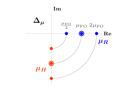
In the limit where the resummation is turned off, this reproduces the perturbative uncertainty in the fixed-order predictions. For the resummed predictions, the magnitude of the hard scale by construction follows the $\mu_{\mathrm{FO}}$ variation, $|\mu_{H}|=\mu_{\mathrm{FO}}$, as illustrated in fig. 1 on the left, such that the fixed-order variations do not change the resummed logarithms $\ln(\mu_{H}/\mu_{\mathrm{FO}})$.

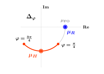
For the resummation uncertainty, we vary the phase $\varphi$ in the interval $[\pi/4,3\pi/4]$ around the central value of $\varphi=\pi/2$, while keeping $\mu_{\mathrm{FO}}$ at its central value, as illustrated in fig. 1 on the right. This probes the intrinsic size of the higher-order timelike logarithms. The phase variation by $\pm\pi/4$ is chosen to be roughly equivalent to the usual factor of 2 for conventional logarithms since $\pi/4\simeq\ln 2$. The uncertainty $\Delta_{\varphi}$ is then obtained as the maximum observed deviation from the central value (usually happening at one of the endpoints), such that

$$\Delta_{\varphi}=\max_{\varphi\in[\pi/4,\,3\pi/4]}\bigl{\lvert}\sigma_{\rm vary}(\varphi)-\sigma_{\rm central}\bigr{\rvert}\,.$$ (18)

This additional resummation uncertainty was not considered in earlier treatments, but has already been included in the resummed 0/1/2-jet-bin results reported in ref. deFlorian:2016spz .

The total perturbative uncertainty is obtained by adding the two independent sources,

$$\Delta_{\mu}\oplus\Delta_{\varphi}=\sqrt{\Delta_{\mu}^{2}+\Delta_{\varphi}^{2}}\,.$$ (19)

For $b\bar{b}\to H$ we follow ref. Bonvini:2016fgf and consider the low-scale matching at $\mu_{b}$ onto the $b$-quark PDFs as a third independent source of uncertainty $\Delta_{b}$, which is estimated by varying $\mu_{b}$ by a factor of two.

Figure 1: Illustration of the scale variations used to estimate the perturbative uncertainties. Left: The overall variations of $\mu_{\mathrm{FO}}$, which determines $\Delta_{\mu}$ (in conjunction with the variation of $\kappa_{F}$, which is not shown). Right: The phase variation for $\mu_{H}$ for fixed $\mu_{\mathrm{FO}}$, which determines the resummation uncertainty $\Delta_{\varphi}$.

3 Gluon fusion

Gluon-fusion processes are well-known to contain large perturbative corrections, which are partially due to the timelike logarithms in the gluon form factor, as first demonstrated in ref. Ahrens:2008qu . We first consider the total production cross section up to N³LO+$\text{N\textsuperscript{3}LL}^{\prime}_{\varphi}$ for a generic scalar final state $gg\to X$ in sec. 3.1 and for the SM Higgs boson in the rEFT $m_{t}\to\infty$ limit in sec. 3.2. In sec. 3.3 we discuss how to incorporate quark-mass and electroweak effects into the resummed results. In sec. 3.4 we then present our results for the Higgs rapidity spectrum and the cross section with a rapidity cut to NNLO+$\text{NNLL}^{\prime}_{\varphi}$.

3.1 Color-singlet production

We first consider the total production cross section from gluon fusion for a generic color-singlet scalar $X$ with mass $m_{X}$. Its coupling to gluons at the scale $\mu\sim m_{X}$ can be expressed in terms of an effective Lagrangian as

$$\mathcal{L}_{\text{eff}}(m_{X})\supset-\frac{C_{X}}{\Lambda}\,\alpha_{s}\,G_{\mu\nu}^{a}G^{a,\mu\nu}X\,,$$ (20)

where $\Lambda$ is a suitable high mass scale and $C_{X}$ is the Wilson coefficient from integrating out heavy particles that mediate the effective $ggX$ interaction. This effective operator arises for SM Higgs production in the $m_{t}\to\infty$ limit, which we discuss in more detail in sec. 3.2. Here, we use it as a simple case to study the effects of the resummation and its dependence on the mass over a wide range $m_{X}\in[100,1000]\,\mathrm{GeV}$. For this purpose, the precise values of the effective coupling $C_{X}(\mu=m_{X})/\Lambda$ need not be specified, as it drops out for the $K$-factor $\sigma/\sigma^{(0)}$ on which the resummation acts.

We obtain the total $gg\rightarrow X$ cross section to N³LO from SusHi 1.6.0 Harlander:2002wh ; Harlander:2005rq ; Harlander:2012pb ; Harlander:2016hcx ; Chetyrkin:2000yt ; Anastasiou:2014lda ; Anastasiou:2015yha ; Anastasiou:2016cez . Our central scale choices are $\mu_{\mathrm{FO}}=m_{X}$ and $\kappa_{F}=1$, such that $\mu_{R}=\mu_{F}=m_{X}$. Away from $\mu=m_{X}$, the perturbative running of $C_{X}(\mu)$ induces logarithms of $m_{X}/\mu$ at NNLO and N³LO. Their resummation is irrelevant and can be neglected, and they are instead included in the fixed-order cross section Harlander:2016hcx .

The gluon form factor is known up to three loops Harlander:2000mg ; Gehrmann:2005pd ; Moch:2005tm ; Baikov:2009bg ; Lee:2010cga ; Gehrmann:2010ue , and the Wilson coefficient $C_{gg}$ is explicitly extracted from it in ref. Gehrmann:2010ue (see also refs. Idilbi:2005ni ; Idilbi:2006dg ),

$$H_{gg}(m_{X}^{2},\mu)=\bigl{|}C_{gg}(m_{X}^{2},\mu)\bigr{|}^{2}=\biggl{|}1+\sum_{n=1}^{\infty}\biggl{[}\frac{\alpha_{s}(\mu)}{4\pi}\biggr{]}^{n}C_{gg}^{(n)}\biggl{(}\ln\frac{-m_{X}^{2}-\mathrm{i}0}{\mu^{2}}\biggr{)}\biggr{|}^{2}\,,$$ (21)

where now $Q^{2}=m_{X}^{2}$. The RGE of $C_{gg}$ reads

$$\mu\frac{\mathrm{d}}{\mathrm{d}\mu}C_{gg}(m_{X}^{2},\mu) =\gamma_{gg}(m_{X}^{2},\mu)\,C_{gg}(m_{X}^{2},\mu)\,,$$ (22)

$$\gamma_{gg}(m_{X}^{2},\mu) =\Gamma^{g}_{\mathrm{cusp}}[\alpha_{s}(\mu)]\ln\frac{-m_{X}^{2}-\mathrm{i}0}{\mu^{2}}+2\gamma_{C}^{g}[\alpha_{s}(\mu)]-\gamma_{t}[\alpha_{s}(\mu)]-\frac{\beta[\alpha_{s}(\mu)]}{\alpha_{s}(\mu)}\,,$$

where $\Gamma^{g}_{\mathrm{cusp}}(\alpha_{s})$ is the gluon cusp anomalous dimension and the last three terms are the total noncusp contribution. All the relevant ingredients are collected in appendix A.

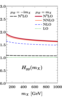
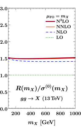
The separation of the perturbative series for the $K$ factor at fixed order into those of $H$ and $R$ is shown in fig. 2 as a function of $m_{X}$. Half of the large NLO $K$ factor comes from $H$ and half from $R$, while beyond NLO the corrections in $H$ are larger than for $R$. Hence, the large corrections to the $K$-factor present at each order are driven to a large extent (but also not entirely) by the corrections from $H$. In particular, the remainder $R$ by itself has a much better behaved perturbative series than $K$, and there are clearly no cancellations between $H$ and $R$. (Otherwise, as already explained in sec. 2.1, $R$ would need to have negative corrections that are larger in size than those in $K$.) This pattern holds independently of $m_{X}$. The visible increase in the corrections toward smaller $m_{X}$ is due to the running of $\alpha_{s}(m_{X})$.

The large perturbative corrections in $H_{gg}$ at the real scale $\mu_{H}=m_{X}$ are absent at the imaginary scale $\mu_{H}=-\mathrm{i}m_{X}$, as shown by the long-dashed curve in the middle panel of fig. 2. To illustrate this more explicitly, the numerical values for an example mass of $m_{X}=750\,\mathrm{GeV}$ are,

$$H_{gg}(m_{X}^{2},\mu_{H}=m_{X}) =1+0.49279+0.13855+0.02288\,,$$

$$H_{gg}(m_{X}^{2},\mu_{H}=-\mathrm{i}m_{X}) =1+0.06820-0.00102-0.00251\,,$$ (23)

where each term is the contribution from a subsequent order in $\alpha_{s}$ up to N³LO. Clearly, the large corrections to the gluon form factor at real scales are almost entirely due to the timelike Sudakov logarithms that are present for $\mu_{H}=m_{X}$ and are eliminated by taking $\mu_{H}=-\mathrm{i}m_{X}$. Since the corrections in $H_{gg}$ at $\mu_{H}=-\mathrm{i}m_{X}$ are very small, the perturbative convergence of the resummed cross section will be essentially determined by that of the remainder $R$.

Figure 2: Illustration of the fixed-order perturbative series for $gg\rightarrow X$ at $\mu_{\mathrm{FO}}=m_{X}$ for the inclusive $K$-factor (left), the hard function $H_{gg}$ at $\mu_{H}=m_{X}$ (center), and the normalized remainder $R/\sigma^{(0)}$ (right). The middle panel also shows the N³LO hard function $H_{gg}$ at $\mu_{H}=-\mathrm{i}m_{X}$ (black long dashed), for which it contains no timelike logarithms.

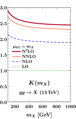
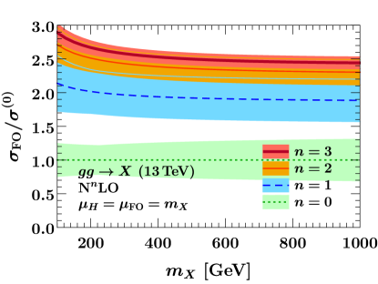
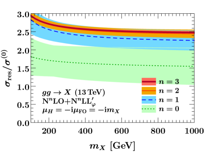
In fig. 3, we compare the fixed-order and resummed cross sections as a function of $m_{X}$, with the bands showing the total perturbative uncertainties evaluated as discussed in sec. 2.2. (Note that in case of $gg\rightarrow X$ and $gg\rightarrow H$, the fixed-order uncertainties come from the variation of $\mu_{R}$ for fixed $\mu_{F}$.) All results are normalized to the LO prediction $\sigma^{(0)}$ at fixed $\mu_{\mathrm{FO}}=m_{X}$. As expected, the absence of large corrections in the resummed hard function directly translates into a much faster convergence of the resummed cross section. Furthermore, the uncertainties in the resummed predictions at lower orders cover the higher-order bands much better than at fixed order, while at the same time being substantially reduced at higher orders. Hence, even at NNLO and N³LO, where the fixed-order results start to show convergence, the resummation noticeably improves the predictions. Due to their better convergence, the resummed predictions provide substantially improved uncertainty estimates both in terms of their reliability and their size. In particular, we can be reasonably confident that the result at the next higher order will lie within the small N³LO+$\text{N\textsuperscript{3}LL}^{\prime}_{\varphi}$ uncertainty band.

Figure 3: The total cross section for $gg\rightarrow X$ at $E_{\mathrm{cm}}=13\,\mathrm{TeV}$ at fixed order (left) and including the resummation of timelike logarithms (right). All results are normalized to the central LO prediction at $\mu_{\mathrm{FO}}=m_{X}$.

3.2 Inclusive Higgs production in the rEFT scheme

We now turn to the case of Higgs production through gluon fusion as an important application of the singlet production discussed above. For Higgs masses below the top threshold, $m_{H}<2m_{t}$, the gluon-fusion cross section can be well approximated by an effective theory where the top quark is integrated out Wilczek:1977zn ; Shifman:1978zn ; Inami:1982xt ; Spiridonov:1988md , giving rise to an effective Lagrangian analogous to eq. (20),

$$\mathcal{L}(m_{H})\supset-\frac{C_{t}}{12\pi v}\,\alpha_{s}\,G_{\mu\nu}^{a}G^{a,\mu\nu}H\,.$$ (24)

In this case, the Wilson coefficient $C_{t}$ itself receives sizable QCD corrections, which have been calculated to N⁴LO in refs. Chetyrkin:1997un ; Schroder:2005hy ; Chetyrkin:2005ia . The effective operator in eq. (24) is the same as in eq. (20), giving rise to the same gluon form factor and hard function $H_{gg}$ in eq. (21).

Rescaling the cross section $\sigma^{\mathrm{EFT}}$ obtained from eq. (24) by the LO $m_{t}$ dependence Georgi:1977gs

$$F_{0}(\rho)=\frac{3}{2\rho}-\frac{3}{2\rho}\biggl{|}1-\frac{1}{\rho}\biggr{|}\arcsin^{2}(\sqrt{\rho})\,,\qquad\rho=\frac{m_{H}^{2}}{4m_{t}^{2}}<1\,,$$ (25)

one obtains the inclusive cross section in the “rescaled EFT” scheme (rEFT),

$$\sigma^{\mathrm{rEFT}}=|F_{0}(\rho)|^{2}\,\sigma^{\mathrm{EFT}}\,.$$ (26)

This rescaling is known to well reproduce the $m_{t}$-exact result at NLO, and hence it is believed to be a useful approximation also at higher orders Graudenz:1992pv ; Dawson:1993qf ; Spira:1995rr ; Harlander:2009bw ; Pak:2009bx ; Harlander:2009mq ; Pak:2009dg ; Harlander:2009my . The inclusion of further quark mass and electroweak effects will be discussed in sec. 3.3.

We use SusHi 1.6.0 Harlander:2002wh ; Harlander:2005rq ; Harlander:2012pb ; Harlander:2016hcx ; Chetyrkin:2000yt to compute the total cross section in the rEFT scheme to NNLO. For the N³LO contribution we use the results of ref. Anastasiou:2016cez as implemented in ggHiggs 3.5 Bonvini:2016frm . We use $m_{t}^{\mathrm{OS}}=172.5\,\mathrm{GeV}$ and $m_{H}=125\,\mathrm{GeV}$. To study the perturbative series and the resummation effects we choose the canonical values $\mu_{\mathrm{FO}}=m_{H}$ and $\kappa_{F}=1$ (so $\mu_{R}=\mu_{F}=m_{H}$) as central values. With these settings, the N³LO cross section has the perturbative series

$$\sigma_{\mathrm{FO}}^{\mathrm{rEFT}} =(1+1.291+0.783+0.296)\times 13.80\,\mathrm{pb}\,,$$

$$H_{gg}(m_{H}^{2},\mu_{H}=m_{H}) =\,\,1+0.619+0.219+0.045\,,$$

$$R(\mu_{\mathrm{FO}}=m_{H}) =(1+0.672+0.148+0.012)\times 13.80\,\mathrm{pb}\,,$$ (27)

where again each term gives the contribution from a subsequent order in $\alpha_{s}$. The remainder $R$ now includes the corrections to $|C_{t}|^{2}$. As before, its perturbative series is much better behaved than that of the cross section, whose large perturbative corrections are thus driven by the large corrections from timelike logarithms in $H_{gg}$.

To illustrate the improved convergence of the resummed form factor, we consider the hard function $H_{gg}(m_{H},\mu_{H})$ at various scales $\mu_{H}$,

$$H_{gg}(m_{H}^{2},\mu_{H}=m_{H}) =1+0.61925+0.21878+0.04539\,,$$

$$H_{gg}(m_{H}^{2},\mu_{H}=-\mathrm{i}m_{H}) =1+0.08408-0.00145-0.00441\,,$$

$$H_{gg}(m_{H}^{2},\mu_{H}=m_{H}/2) =1+0.57325+0.12361-0.00839\,,$$

$$H_{gg}(m_{H}^{2},\mu_{H}=-\mathrm{i}m_{H}/2) =1-0.01553-0.01544-0.00247\,,$$

$$H_{gg}(m_{H}^{2},\mu_{H}=m_{H}/5) =1+0.08090-0.16424-0.00552\,.$$ (28)

For both imaginary-valued scales $\mu_{H}=-\mathrm{i}m_{H}$ and $\mu_{H}=-\mathrm{i}m_{H}/2$, the corrections are drastically reduced compare to the real scale choice. For comparison, choosing a real value $\mu_{H}=m_{H}/5$ that yields the same reduced NLO correction as $\mu_{H}=-\mathrm{i}m_{H}$ still leads to much larger NNLO corrections.

Figure 4: The $gg\rightarrow H$ cross section at $E_{\mathrm{cm}}=13\,\mathrm{TeV}$ and $m_{H}=125\,\mathrm{GeV}$ in the rEFT scheme. Left: The cross section as a function of the resummation phase $\varphi$ of the hard scale $\mu_{H}=\mu_{\mathrm{FO}}\exp(-\mathrm{i}\varphi)$, with the uncertainty bands corresponding to $\Delta_{\mu}$ only. Right: Comparison of the fixed-order results for $\mu_{\mathrm{FO}}=m_{H}$ and $\mu_{\mathrm{FO}}=m_{H}/2$, and the resummed results with $\mu_{\mathrm{FO}}=\mathrm{i}\mu_{H}=m_{H}$. All results are given as the percent difference from the N³LO+$\text{N\textsuperscript{3}LL}^{\prime}_{\varphi}$ central value. The uncertainty bars show $\Delta_{\mu}$ for the fixed-order results and $\Delta_{\mu}\oplus\Delta_{\varphi}$ for the resummed results (with the inner bars visible at the lower orders showing $\Delta_{\varphi}$ only). The fixed LO results are out of range.

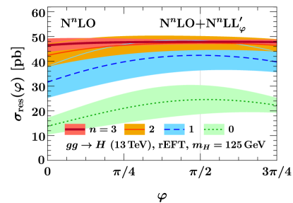
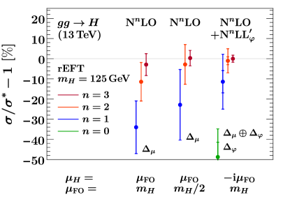
To examine the dependence on the resummation phase $\varphi$ of the hard scale, $\mu_{H}=\mu_{\mathrm{FO}}\exp(-\mathrm{i}\varphi)$, we show in the left panel of fig. 4 the resummed cross section as a function of $\varphi$. Here, the uncertainty bands only show the fixed-order uncertainty $\Delta_{\mu}$. At $\varphi=0$, $\sigma_{\mathrm{res}}(\varphi)$ is just the fixed-order cross section. As $\varphi\rightarrow\pi/2$, the timelike resummation is turned on, visibly improving the convergence of the cross section and providing better coverage of the uncertainty bands. The $\varphi$ dependence becomes stationary at $\varphi=\pi/2$, where the timelike Sudakov logarithms exactly vanish. Beyond $\varphi=\pi/2$, powers of $\varphi-\pi/2$ start to enter again.

In the right panel of fig. 4, we compare the fixed-order results at the conventional scales of $\mu_{\mathrm{FO}}=m_{H}$ and $\mu_{\mathrm{FO}}=m_{H}/2$ with the resummed results. The results are shown as relative corrections to our best prediction at N³LO+$\text{N\textsuperscript{3}LL}^{\prime}_{\varphi}$. For the resummed results, the inner uncertainty bars indicate $\Delta_{\varphi}$ alone, while the outer ones show $\Delta_{\mu}\oplus\Delta_{\varphi}$. While $\Delta_{\varphi}$ contributes to obtaining a more realistic uncertainty estimate at LO+$\text{LL}^{\prime}_{\varphi}$ (compared to LO), its impact is strongly reduced at higher orders. The overall picture and conclusions from the generic color-singlet case are unaffected by the presence of the Wilson coefficient $|C_{t}|^{2}$ in the cross section. The resummation yields again a clear improvement in convergence and uncertainties, also compared to the fixed-order results at $\mu_{\mathrm{FO}}=m_{H}/2$, which are already better behaved than those at $\mu_{\mathrm{FO}}=m_{H}$. In particular, the NLO+$\text{NLL}^{\prime}_{\varphi}$ result already fully covers the highest-order result, which is not the case at fixed NLO, and the precision of the NNLO+$\text{NNLL}^{\prime}_{\varphi}$ result is roughly comparable to the fixed N³LO results. This gives us good confidence in the small remaining uncertainty at N³LO+$\text{N\textsuperscript{3}LL}^{\prime}_{\varphi}$, which is reduced by a factor of two compared to N³LO. The explicit numerical results at the highest order are

$$\sigma_{\mathrm{FO}}^{\mathrm{rEFT}} =(46.51\pm 2.60_{\mu})\,\mathrm{pb}~{} (5.59\%)\,,\quad (\text{\text{N\textsuperscript{3}LO}},\,\mu_{\mathrm{FO}}=m_{H})\,,$$

$$\sigma_{\mathrm{FO}}^{\mathrm{rEFT}} =(48.06\pm 1.83_{\mu})\,\mathrm{pb}~{} (3.82\%)\,,\quad (\text{\text{N\textsuperscript{3}LO}},\,\mu_{\mathrm{FO}}=m_{H}/2)\,,$$

$$\sigma_{\mathrm{res}}^{\mathrm{rEFT}} =(47.90\pm 0.82_{\mu}\pm 0.18_{\varphi})\,\mathrm{pb}~{} (1.75\%)\,,\quad (\text{$\text{N\textsuperscript{3}LO}$+$\text{N\textsuperscript{3}LL}^{\prime}_{\varphi}$},\,\mu_{\mathrm{FO}}=m_{H})\,.$$ (29)

Note that for the N³LO results in ref. Anastasiou:2016cez the perturbative uncertainties are estimated by varying $\mu_{\mathrm{FO}}$ but keeping $\kappa_{F}=1$ fixed. Doing so reduces $\Delta_{\mu}$ to $2.21\,\mathrm{pb}$ $(4.76\%)$ at central $\mu_{\mathrm{FO}}=m_{H}$ and $1.54\,\mathrm{pb}$ $(3.21\%)$ at central $\mu_{\mathrm{FO}}=m_{H}/2$. Similarly dropping the $\kappa_{F}$ variation in the resummed results gives $\Delta_{\mu}=0.67\,\mathrm{pb}$, which combined with $\Delta_{\varphi}$ then yields a total perturbative uncertainty of $1.44\%$. Note also that using the threshold-expanded running in $\mu_{R}$ and $\mu_{F}$ as implemented in SusHi 1.6.0, the N³LO result at $\mu_{\mathrm{FO}}=m_{H}/2$ increases to $(48.17\pm 1.99_{\mu})\,\mathrm{pb}~{}(4.14\%)$, with a corresponding increase in $\Delta_{\mu}$ since the result at $\mu_{\mathrm{FO}}=m_{H}$ is unaffected.

3.3 Incorporating quark mass and electroweak effects beyond rEFT

While the previous section focused on the QCD corrections to Higgs production in the $m_{t}\to\infty$ limit, further corrections arise from finite quark-mass effects as well as electroweak contributions. Here we discuss how to consistently combine them with the resummation of timelike logarithms.

The full dependence of the cross section on the heavy quark masses $m_{t}$, $m_{b}$, $m_{c}$ is fully known at NLO Graudenz:1992pv ; Dawson:1993qf ; Spira:1995rr ; Harlander:2005rq ; Anastasiou:2006hc ; Aglietti:2006tp ; Anastasiou:2009kn . We define $\delta\sigma^{q}_{\text{(N)LO}}$ as the correction of the exact result relative to the rEFT result,

$$\sigma_{\text{NLO}}^{t,b,c} =\sigma^{\mathrm{rEFT}}_{\text{NLO}}+\delta\sigma_{\text{LO}}^{b,c}+\delta\sigma^{t,b,c}_{\text{NLO}}\,.$$ (30)

On top of the exact NLO corrections, top-quark mass effects are also known in an asymptotic expansion in $1/m_{t}$ at NNLO Harlander:2009bw ; Pak:2009bx ; Harlander:2009mq ; Pak:2009dg ; Harlander:2009my .

In the following we consider the top-mass effects in more detail. As discussed in refs. Harlander:2009my ; Harlander:2009mq ; Pak:2009dg ; Harlander:2016hcx , the asymptotic $1/m_{t}$ corrections at NNLO cannot be expected to reliably improve over the $m_{t}\to\infty$ limit. Rather, they can serve to estimate the uncertainty due to the still unknown full NNLO $m_{t}$ corrections. For this reason we will only take into account the NLO corrections $\delta\sigma^{t}_{\text{NLO}}$. (The inclusion of the NNLO $m_{t}$ corrections would be completely analogous.) This is also consistent with our analysis of the rapidity spectrum in sec. 3.4, for which the $m_{t}$-corrections are only known at NLO. For illustration, the numerical results for $\delta\sigma^{t}_{\text{NLO}}$ are

$$\delta\sigma^{t}_{\text{NLO}}=-0.210\,\mathrm{pb}\,,\qquad (\mu_{\mathrm{FO}}=m_{H})\,,$$ (31)

$$\delta\sigma^{t}_{\text{NLO}}=-0.315\,\mathrm{pb}\,, (\mu_{\mathrm{FO}}=m_{H}/2)\,.$$

The finite $m_{t}$ contributions correspond to a correction to the $m_{t}\to\infty$ limit in eq. (24), from which the gluon form factor arises, and so a priori they do not involve the same local gluon form factor. Therefore, one option to include them in the resummed results is to simply add them to the rEFT results in eq. (3.2), which yields

$$\sigma_{\mathrm{FO}}^{\mathrm{rEFT}}+\delta\sigma^{t}_{\text{NLO}}=(46.30\pm 2.55_{\mu})\,\mathrm{pb}~{} (5.50\%)\quad (\text{\text{N\textsuperscript{3}LO}},\,\mu_{\mathrm{FO}}=m_{H})\,,$$

$$\sigma_{\mathrm{FO}}^{\mathrm{rEFT}}+\delta\sigma^{t}_{\text{NLO}}=(47.74\pm 1.75_{\mu})\,\mathrm{pb}~{} (3.66\%)\quad (\text{\text{N\textsuperscript{3}LO}},\,\mu_{\mathrm{FO}}=m_{H}/2)\,,$$ (32)

$$\sigma_{\mathrm{res}}^{\mathrm{rEFT}}+\delta\sigma^{t}_{\text{NLO}}=(47.69\pm 0.78_{\mu}\pm 0.18_{\varphi})\,\mathrm{pb}~{} (1.68\%)\,,\quad (\text{$\text{N\textsuperscript{3}LO}$+$\text{N\textsuperscript{3}LL}^{\prime}_{\varphi}$},\,\mu_{\mathrm{FO}}=m_{H})\,.$$

The complete results including those at lower orders are collected in table 1.

Alternatively, following ref. Berger:2010xi we can perform a one-step matching of the full Standard Model including the top quark onto SCET, simultaneously integrating out both the top quark and hard virtual corrections. The resulting hard function $H_{gg}^{t}=|C_{gg}^{t}|^{2}$ corresponds to the full SM $gg\to H$ form factor and includes all virtual finite-$m_{t}$ effects. It takes the form Berger:2010xi

$$H_{gg}^{t}(m_{t},m_{H}^{2},\mu)=|F_{0}(\rho)|^{2}|\alpha_{s}(\mu)|^{2}\,\Bigl{\{} \bigl{|}C_{t}(m_{t},\mu)\,C_{gg}(m_{H}^{2},\mu)\bigr{|}^{2}$$

$$+2\operatorname{Re}\Bigl{[}\frac{\alpha_{s}(\mu)}{4\pi}(F_{1}(\rho)-F_{1}(0))\Bigr{]}+\mathcal{O}(\rho\,\alpha_{s}^{2})\Bigr{\}}\,,$$ (33)

where as before $\rho\equiv m_{H}^{2}/(4m_{t}^{2})$. Compared to $H_{gg}=|C_{gg}|^{2}$, the LO $m_{t}$ dependence $F_{0}(\rho)$ and the contributions from $C_{t}$ are now moved from the remainder into the hard function. The $F_{1}(\rho)$ contains the full virtual $m_{t}$ dependence at NLO and the $\mathcal{O}(\rho\,\alpha_{s}^{2})$ terms denote the neglected NNLO virtual $m_{t}$ corrections. Although $H_{gg}^{t}$ is no longer normalized to unity at leading order, we can continue to use eq. (12) to obtain the resummed cross section. Compared to eq. (11), the result now contains an overall factor $|\alpha_{s}(\mu_{H})/\alpha_{s}(\mu_{\mathrm{FO}})|^{2}$ from the ratio of hard functions, which replaces the $\alpha_{s}^{2}(\mu_{\mathrm{FO}})$ inside the LO cross section by $|\alpha_{s}(\mu_{H})|^{2}$.

The RGE for $C_{gg}^{t}$ is given by

$$\mu\frac{\mathrm{d}}{\mathrm{d}\mu}C_{gg}^{t}(m_{t},m_{H}^{2},\mu) =\gamma_{gg}^{t}(m_{H}^{2},\mu)\,C_{gg}^{t}(m_{t},m_{H}^{2},\mu)\,,$$

$$\gamma_{gg}^{t}(m_{H}^{2},\mu) =\Gamma^{g}_{\mathrm{cusp}}[\alpha_{s}(\mu)]\ln\frac{-m_{H}^{2}-\mathrm{i}0}{\mu^{2}}+2\gamma_{C}^{g}[\alpha_{s}(\mu)]\,.$$ (34)

The noncusp terms in $\gamma_{gg}^{t}$ differ from those in $\gamma_{gg}$ in eq. (22) due to the additional $\mu$ dependence of $\alpha_{s}(\mu)C_{t}(\mu)$, which is now included in the hard Wilson coefficient. The overall $|\alpha_{s}(\mu)|^{2}|C_{t}(m_{t},\mu)|^{2}$ in eq. (3.3) is now evaluated at $\mu_{H}=-\mathrm{i}\mu_{\mathrm{FO}}$ and then evolved back to $\mu_{\mathrm{FO}}$. For the overall $\alpha_{s}(\mu)$ this is largely irrelevant since it is ultimately evolved starting from $\alpha_{s}(m_{Z})$. For $C_{t}(\mu)$, which is treated in fixed order, this induces different subleading timelike logarithms starting at NNLO compared to $H_{gg}$. This is reflected in the noncusp terms differing by $\gamma_{t}$, whose numerical effect however is not significant. Also, the perturbative convergence of $|C_{t}(\mu)|^{2}$ at $\mu=m_{H}$ and $\mu=-\mathrm{i}m_{H}$ (and at its natural scale $\mu=m_{t}$) is practically the same.

The perturbative convergence of $H_{gg}^{t}$ shows the same improvement as seen for $H_{gg}$ when evaluated at $\mu_{H}=-\mathrm{i}m_{H}$ rather than $\mu_{H}=m_{H}$,

$$H_{gg}^{t}(m_{H},\mu_{H}=m_{H}) =|\alpha_{s}(m_{H})|^{2}\,|F_{0}|^{2} \times\,\bigl{(}1+0.82152+0.36170+0.10268\bigr{)}\,,$$

$$H_{gg}^{t}(m_{H},\mu_{H}=-\mathrm{i}m_{H}) =|\alpha_{s}(-\mathrm{i}m_{H})|^{2}\,|F_{0}|^{2} \times\,\bigl{(}1+0.27631+0.04244-0.00257\bigr{)}\,.$$ (35)

The main difference compared to $H_{gg}$ are the additional constant terms from $C_{t}$ that are now included in $H_{gg}^{t}$. The finite-$m_{t}$ corrections have a very small effect on the NLO contribution, contributing a $+0.005$ to the above $0.82152$ and $0.27631$.

For reference, we first consider the rEFT limit and drop the finite-$m_{t}$ terms in $H_{gg}^{t}$ as well as $\delta\sigma_{\text{NLO}}^{t}$. The rEFT result based on $H_{gg}^{t}$ at N³LO+$\text{N\textsuperscript{3}LL}^{\prime}_{\varphi}$ then reads

$$\sigma_{\mathrm{res},\,H^{t}}^{\mathrm{rEFT}}=(47.98\pm 0.85_{\mu}\pm 0.24_{\varphi})\,\mathrm{pb}~{}(1.85\%)\,.$$ (36)

This is equivalent to the results at $\mu_{H}=-\mathrm{i}m_{H}$ reported in ref. deFlorian:2016spz . Including the full NLO $m_{t}$ dependence, we obtain

$$\left(\sigma^{\mathrm{rEFT}}+\delta\sigma^{t}_{\text{NLO}}\right)_{\mathrm{res},\,H^{t}}=(47.84\pm 0.81_{\mu}\pm 0.25_{\varphi})\,\mathrm{pb}~{}(1.77\%)\,.$$ (37)

The full set of results including the lower orders are shown in the last column of table 1.

$\sigma\,[\!\,\mathrm{pb}]$ for $gg\to H$, $E_{\mathrm{cm}}=13\,\mathrm{TeV}$, $m_{H}=125\,\mathrm{GeV}$
	$\sigma^{\mathrm{rEFT}}_{\mathrm{FO}}\!+\delta\sigma^{t}_{\text{NLO}}$		$\sigma^{\mathrm{rEFT}}_{\mathrm{res}}\!+\delta\sigma^{t}_{\text{NLO}}$	$(\sigma^{\mathrm{rEFT}}+\delta\sigma^{t}_{\text{NLO}})_{\mathrm{res}}$
$n$	$\text{N\textsuperscript{$n$}LO},\,\mu_{\mathrm{FO}}=m_{H}$	$\text{N\textsuperscript{$n$}LO},\,\mu_{\mathrm{FO}}=\frac{m_{H}}{2}$	N$n$LO+$\text{N\textsuperscript{$n$}LL}^{\prime}_{\varphi}\,\,(H_{gg})$	N$n$LO+$\text{N\textsuperscript{$n$}LL}^{\prime}_{\varphi}\,\,(H^{t}_{gg})$
$0$	$13.8\!\pm\!3.2_{\mu}\,(23\%)$	$16.0\!\pm\!4.3_{\mu}\,(27\%)$	$24.5\!\pm\!5.7_{\mu}\!\pm\!3.5_{\varphi}\,(27\%)$	$23.3\!\pm\!5.1_{\mu}\!\pm\!3.4_{\varphi}\,(26\%)$
$1$	$31.4\!\pm\!6.2_{\mu}\,(20\%)$	$36.6\!\pm\!8.2_{\mu}\,(23\%)$	$42.2\!\pm\!5.9_{\mu}\!\pm\!2.7_{\varphi}\,(15\%)$	$41.8\!\pm\!5.7_{\mu}\!\pm\!2.8_{\varphi}\,(15\%)$
$2$	$42.2\!\pm\!4.5_{\mu}\,(11\%)$	$46.2\!\pm\!4.6_{\mu}\,(10\%)$	$47.2\!\pm\!2.6_{\mu}\!\pm\!1.0_{\varphi}\,(6.0\%)$	$47.3\!\pm\!2.7_{\mu}\!\pm\!1.0_{\varphi}\,(6.1\%)$
$3$	$46.3\!\pm\!2.5_{\mu}\,(5.5\%)$	$47.7\!\pm\!1.7_{\mu}\,(3.7\%)$	$47.7\!\pm\!0.8_{\mu}\!\pm\!0.18_{\varphi}\,(1.7\%)$	$47.8\!\pm\!0.8_{\mu}\!\pm\!0.25_{\varphi}\,(1.8\%)$

Table 1: Total $gg\rightarrow H$ cross section at $E_{\mathrm{cm}}=13\,\mathrm{TeV}$ and $m_{H}=125\,\mathrm{GeV}$. All results include the exact $m_{t}$ dependence $\delta\sigma^{t}$ at NLO. The percent uncertainties for the resummed results correspond to the total uncertainty $\Delta_{\mu}\oplus\Delta_{\varphi}$.

Comparing the last two columns of table 1, the resummed results using the two different ways to include the top-quark contributions are perfectly compatible with each other. The fixed-order uncertainty is essentially unaffected, because it is insensitive to the precise split of the constant terms into $H$ and $R$ due to the reexpansion of their fixed-order contributions [see eq. (11)]. The resummation uncertainty $\Delta_{\varphi}$ increases somewhat in the one-step matching, which reflects the fact that the $C_{t}$ contributions introduce an additional residual $\mu$ dependence and that they are evaluated at $\mu=-\mathrm{i}m_{H}$ rather than their natural scale $\mu=m_{t}$. Overall, the numerical differences are however completely insignificant, which shows that the results are insensitive to the precise treatment of the top contributions. This also provides nontrivial verification that the scheme dependence in how the nonlogarithmic constant terms are split between $H$ and $R$ at each order is much smaller than the perturbative uncertainties and hence irrelevant.

A complete numerical inclusion of all known corrections beyond the rEFT limit is beyond the scope of this paper. The inclusion of $b$-quark and electroweak effects can proceed completely analogously to the treatment of the top contributions. Any multiplicative contributions can be trivially included, while additive corrections such as the NLO $m_{b}$-dependent terms can be treated analogously to the finite-$m_{t}$ corrections. For example, the dominant known electroweak corrections can be included by replacing Anastasiou:2008tj

$$C_{t}\to C_{t}+\delta_{\mathrm{EW}}(1+C_{1w}\alpha_{s}+\cdots)\,,$$ (38)

where $\delta_{\text{EW}}$ is the pure NLO electroweak correction to the LO cross section Aglietti:2004nj ; Actis:2008ug and $C_{1w}$ contains the mixed $\mathcal{O}(\alpha\alpha_{s})$ correction calculated in ref. Anastasiou:2008tj by integrating out $W$- and $Z$-bosons as an estimate of the full $\mathcal{O}(\alpha\alpha_{s})$ corrections. These additional contributions will not affect the benefit of the resummation, in the same way the inclusion of the top corrections for $gg\to H$ did not affect the conclusions compared to the generic scalar $gg\to X$ case.

3.4 Higgs rapidity spectrum

As discussed in sec. 2.1, the resummed form factor can be incorporated in the same way as for the total production cross section into generic cross sections that are differential in or contain cuts on the Born kinematics. Here we consider the primary example of the rapidity spectrum as well as the cross section with a rapidity cut. For simplicity we do not consider additional fiducial cuts on the Higgs decay products here, but stress again that these are straightforward to include.

Figure 5: The perturbative remainder $R(Y)/\sigma^{(0)}(Y)$ as a function of the Higgs rapidity $Y$ normalized to the LO spectrum $\sigma^{(0)}(Y)\equiv\mathrm{d}\sigma^{(0)}/\mathrm{d}Y$ in the rEFT limit for $\mu_{\mathrm{FO}}=m_{H}$ (left) and $\mu_{\mathrm{FO}}=m_{H}/2$ (right).

Figure 6: The rapidity distribution for $gg\rightarrow H$ at $E_{\mathrm{cm}}=13\,\mathrm{TeV}$ and $m_{H}=125\,\mathrm{GeV}$ in the rEFT limit. The fixed-order results are shown in the top row at $\mu_{\mathrm{FO}}=m_{H}$ (left) and $\mu_{\mathrm{FO}}=m_{H}/2$ (right). The resummed result is shown on the bottom. The uncertainty bands indicate $\Delta_{\mu}$ and $\Delta_{\mu}\oplus\Delta_{\varphi}$, respectively.

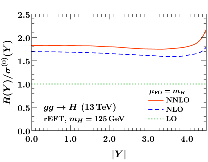
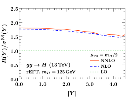
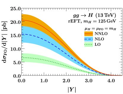
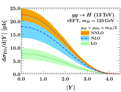
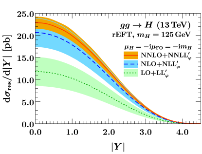
The rapidity spectrum for gluon-fusion Higgs production is known to NNLO Anastasiou:2004xq ; Anastasiou:2005qj ; Anastasiou:2007mz ; Catani:2007vq ; Grazzini:2008tf , while the N³LO corrections are available in the threshold limit Ravindran:2006bu ; Ahmed:2014uya . The resummation in the small-$x$ limit is also known Caola:2010kv . We obtain the fixed-order bin-integrated rapidity distribution for $gg\to H$ to NNLO with HNNLO 2.0 Catani:2007vq ; Grazzini:2008tf . We use a binsize of $\Delta Y=0.25$ and for clarity in all plots interpolate the binned results.

We first consider the rEFT limit and exclude additional quark mass effects. In fig. 5, we display the perturbative remainder $R(Y)$ as a function of $Y$. Although it has some intrinsic nontrivial rapidity dependence, the overall behavior is as for the total cross section, namely it exhibits a noticeably better convergence than the full fixed-order spectrum. Hence, we expect a similar improvement from applying the resummation to the rapidity spectrum as for the total cross section.

The upper panels of fig. 6 show the fixed-order results at $\mu_{\mathrm{FO}}=m_{H}$ and $\mu_{\mathrm{FO}}=m_{H}/2$, with the bands showing $\Delta_{\mu}$. The overall $K$ factor at NLO and NNLO is roughly constant in the central rapidity range and similar to that of the total cross section. This is consistent with the fact that a large part of the $K$ factor stems from the timelike logarithms in the gluon form factor, which is independent of the rapidity.

The resummed result including fixed-order and resummation uncertainties, $\Delta_{\mu}\oplus\Delta_{\varphi}$, is shown in the bottom panel of fig. 6. Clearly, resumming the timelike logarithms improves the perturbative convergence across the spectrum as it did for the total cross section. The NNLO+$\text{NNLL}^{\prime}_{\varphi}$ result has perturbative uncertainties that are almost a factor of two smaller than at NNLO. At the same time, the NNLO+$\text{NNLL}^{\prime}_{\varphi}$ result is well covered by the lower-order NLO+$\text{NLL}^{\prime}_{\varphi}$ uncertainty band, which is not the case at fixed order. Judging from the results for the total cross section, for which the full N³LO is known, we expect the precision of the NNLO+$\text{NNLL}^{\prime}_{\varphi}$ to be roughly comparable to what can be expected for the full N³LO result, and we can be confident that the corresponding N³LO+$\text{N\textsuperscript{3}LL}^{\prime}_{\varphi}$ result will have further reduced uncertainties and will be well contained within the current NNLO+$\text{NNLL}^{\prime}_{\varphi}$ uncertainties.

Next, we consider the cross section with a rapidity cut,

$$\sigma(Y_{\mathrm{cut}})=\int_{0}^{Y_{\mathrm{cut}}}\!\mathrm{d}|Y|\,\frac{\mathrm{d}\sigma}{\mathrm{d}|Y|}\,.$$ (39)

We now also include the exact $m_{t}$-dependence at NLO using HNNLO 2.0 Grazzini:2013mca , from which we extract the rapidity-dependent analogue of $\delta\sigma_{\text{NLO}}^{t}$ in eq. (30). The latter is included in the resummed results as discussed in the previous subsection: It is either added to the resummed result based on $H_{gg}$ giving $\mathrm{d}(\sigma_{\mathrm{res}}+\delta\sigma^{t})/\mathrm{d}Y$. Alternatively, we can apply the resummation to the full $m_{t}$-exact spectrum $\mathrm{d}(\sigma^{\mathrm{rEFT}}+\delta\sigma^{t})_{\mathrm{res}}/\mathrm{d}Y$ using $H_{gg}^{t}$. The obtained differential rapidity spectra look extremely similar to those in fig. 6, since the finite-$m_{t}$ correction yields a small negative shift $-0.2\,\mathrm{pb}<\mathrm{d}(\delta\sigma^{t})/\mathrm{d}Y<0$ throughout.

$\sigma(Y_{\mathrm{cut}}=2.5)\,[\!\,\mathrm{pb}]$ for $gg\to H$, $E_{\mathrm{cm}}=13\,\mathrm{TeV}$, $m_{H}=125\,\mathrm{GeV}$
	$\sigma^{\mathrm{rEFT}}_{\mathrm{FO}}\!+\delta\sigma^{t}_{\text{NLO}}$		$\sigma^{\mathrm{rEFT}}_{\mathrm{res}}\!+\delta\sigma^{t}_{\text{NLO}}$	$(\sigma^{\mathrm{rEFT}}+\delta\sigma^{t}_{\text{NLO}})_{\mathrm{res}}$
$n$	$\text{N\textsuperscript{$n$}LO},\,\mu_{\mathrm{FO}}=m_{H}$	$\text{N\textsuperscript{$n$}LO},\,\mu_{\mathrm{FO}}=\frac{m_{H}}{2}$	N$n$LO+$\text{N\textsuperscript{$n$}LL}^{\prime}_{\varphi}\,\,(H_{gg})$	N$n$LO+$\text{N\textsuperscript{$n$}LL}^{\prime}_{\varphi}\,\,(H^{t}_{gg})$
$0$	$12.5\!\pm\!2.9_{\mu}\,(23\%)$	$14.5\!\pm\!3.9_{\mu}\,(27\%)$	$22.2\!\pm\!5.2_{\mu}\!\pm\!3.2_{\varphi}\,(27\%)$	$21.1\!\pm\!4.6_{\mu}\!\pm\!3.1_{\varphi}\,(26\%)$
$1$	$28.5\!\pm\!5.6_{\mu}\,(20\%)$	$33.3\!\pm\!7.5_{\mu}\,(23\%)$	$38.4\!\pm\!5.4_{\mu}\!\pm\!2.4_{\varphi}\,(15\%)$	$38.0\!\pm\!5.2_{\mu}\!\pm\!2.6_{\varphi}\,(15\%)$
$2$	$38.3\!\pm\!4.0_{\mu}\,(11\%)$	$41.9\!\pm\!4.2_{\mu}\,(10\%)$	$42.8\!\pm\!2.3_{\mu}\!\pm\!0.9_{\varphi}\,(5.8\%)$	$42.9\!\pm\!2.4_{\mu}\!\pm\!0.9_{\varphi}\,(6.0\%)$
$3$	$\approx 42.0$	$\approx 43.2$	$\approx 43.2$	$\approx 43.3$

Table 2: Cross section for $gg\rightarrow H$ with a rapidity cut of $Y_{\mathrm{cut}}=2.5$. All results include the exact $m_{t}$ dependence $\delta\sigma^{t}(Y_{\mathrm{cut}})$ at NLO. The percent uncertainties for the resummed results correspond to the total uncertainty $\Delta_{\mu}\oplus\Delta_{\varphi}$. The approximate $n=3$ results are constructed as explained in the text and are given for illustration only.

In table 2, we provide benchmark results for $Y_{\mathrm{cut}}=2.5$ at fixed order and including resummation. As expected, the resummed results show the same improved convergence and perturbative uncertainties as the rapidity spectrum and the total cross section.

Since the full N³LO rapidity spectrum is not yet known, one might think about approximating it by rescaling the NNLO spectrum to the inclusive N³LO cross section, e.g., by taking $\sigma_{\text{N\textsuperscript{3}LO}}(Y_{\mathrm{cut}})\approx(\sigma_{\text{N\textsuperscript{3}LO}}/\sigma_{\text{NNLO}})\times\sigma_{\text{NNLO}}(Y_{\mathrm{cut}})$. Although this likely improves the central value by moving it closer to the correct result, it is unclear what uncertainties one should assign. In fact, the resummed NNLO+$\text{NNLL}^{\prime}_{\varphi}$ result for the rapidity spectrum provides a clean way to essentially achieve this goal, because it includes the dominant part of the inclusive N³LO $K$ factor, and it does so with the correct rapidity dependence and reliable uncertainties, which are already substantially reduced compared to NNLO.

To illustrate this, first note that the entire rapidity dependence is contained in the remainder $R$. Looking at fig. 5, one might assume that the N³LO contribution is roughly flat in rapidity such that taking

$$R^{(3)}(Y)\approx\frac{R^{(3)}}{\sigma^{(0)}}\,\sigma^{(0)}(Y)\,,\qquad R^{(3)}(Y_{\mathrm{cut}})\approx\frac{R^{(3)}}{\sigma^{(0)}}\,\sigma^{(0)}(Y_{\mathrm{cut}})\,,$$ (40)

provides a reasonable approximation, where $R^{(3)}/\sigma^{(0)}$ is the N³LO correction for the total cross section. Using eq. (40) as input and combining it with the known $H^{(3)}$ and lower-order results we obtain the approximate numbers at N³LO and N³LO+$\text{N\textsuperscript{3}LL}^{\prime}_{\varphi}$ shown in the last line of table 2. As expected, the NNLO+$\text{NNLL}^{\prime}_{\varphi}$ results indeed capture most of the expected shift from the NNLO result. Using the same procedure to evaluate the scale variations, we can project that the relative uncertainties will be similar to the inclusive cross section, namely around 4% at N³LO and around 2% at N³LO+$\text{N\textsuperscript{3}LL}^{\prime}_{\varphi}$. However, we caution again that it is debatable whether it is justified to assign these without knowing the exact result.

4 Quark annihilation

We now turn to $q\bar{q}$ annihilation processes, for which the perturbative corrections are typically much smaller than for gluon fusion. For these, timelike Sudakov logarithms still arise in the corresponding quark form factor at timelike momentum transfer and can be resummed to all orders. We apply the resummation to Higgs production through bottom quark annihilation in sec. 4.1 and to the Drell-Yan process in sec. 4.2.

4.1 Higgs production through bottom-quark annihilation

The cross section for Higgs production through bottom-quark annihilation, $b\bar{b}\to H$, is much smaller than for $gg\to H$, but is important phenomenologically as it provides direct access to the bottom-quark Yukawa coupling and can be enhanced in theories beyond the Standard Model.

The hard function for $b\bar{b}\to H$ corresponds to the quark scalar form factor and is obtained from the SCET matching coefficient $C_{q\bar{q}}^{S}(Q^{2},\mu)$ for the scalar current with two massless quarks, see eq. (2.1). The scalar form factor naturally arises in the five-flavor scheme calculation in which the $b$ quark is treated as a massless quark at the hard matching scale, except for its Yukawa coupling $y(\mu)$ to the Higgs, which always has its physical value corresponding to $\overline{m}_{b}(\mu)$. We exclude the Yukawa coupling from the hard matching coefficient, just as we excluded the overall $|\alpha_{s}C_{X}|^{2}$ for gluon fusion.

To the best of our knowledge, $C_{q\bar{q}}^{S}$ is not yet directly available in the literature. We extract it in appendix A.3.4 to N³LO from the three-loop massless quark scalar form factor calculated in ref. Gehrmann:2014vha (see also refs. Harlander:2003ai ; Ravindran:2006cg ; Anastasiou:2011qx for the NNLO form factor, and ref. Bernreuther:2005gw for the NNLO form factor including the full mass dependence). The RGE of $C_{q\bar{q}}^{S}$ is given by

$$\mu\frac{\mathrm{d}}{\mathrm{d}\mu}C_{q\bar{q}}^{S}(m_{H}^{2},\mu) =\gamma_{q\bar{q}}^{S}(m_{H}^{2},\mu)\,C_{q\bar{q}}^{S}(m_{H}^{2},\mu)\,,$$

$$\gamma_{q\bar{q}}^{S}(m_{H}^{2},\mu) =\Gamma^{q}_{\mathrm{cusp}}[\alpha_{s}(\mu)]\ln\frac{-m_{H}^{2}-\mathrm{i}0}{\mu^{2}}+2\gamma_{C}^{q}[\alpha_{s}(\mu)]-\gamma_{m}[\alpha_{s}(\mu)]\,.$$ (41)

where $\Gamma^{q}_{\mathrm{cusp}}$ is the quark cusp anomalous dimension, and the last two terms are the total noncusp contribution, where $2\gamma_{C}^{q}$ is the usual hard quark noncusp anomalous dimension (also appearing for the vector current) and $\gamma_{m}$ is the mass anomalous dimension of the Yukawa coupling.

We obtain the $b\bar{b}\to H$ total cross section to NNLO in the five-flavor scheme Barnett:1987jw ; Dicus:1988cx from SusHi 1.6.0 Chetyrkin:2000yt ; Harlander:2002wh ; Harlander:2003ai ; Harlander:2012pb ; Harlander:2016hcx . The Yukawa coupling is evaluated at $\mu_{\mathrm{FO}}$ and obtained by evolving from $\overline{m}_{b}(\overline{m}_{b})=4.18\,\mathrm{GeV}$ using three-loop running. We use the reevolved five-flavor PDF4LHC PDF sets from refs. Bonvini:2015pxa ; Bonvini:2016fgf , which use a $b$-quark pole mass for the $b$ PDF that is consistent with our choice of $\overline{m}_{b}(\overline{m}_{b})$ (namely the one-loop pole mass $m_{b}=4.58\,\mathrm{GeV}$). These PDF sets also distinguish the $b$-quark matching scale $\mu_{b}$ from the physical mass parameter $m_{b}$, allowing to estimate the perturbative uncertainty $\Delta_{b}$ associated with the low-scale matching onto the $b$-quark PDFs by varying $\mu_{b}$ (see ref. Bonvini:2016fgf for details). For the central value we use $\mu_{b}=m_{b}$.

In contrast to the gluon-initiated case, here the $\mu_{F}$ dependence of the cross section plays the dominant role, while the $\mu_{R}$ dependence is much less important. For our central scales we use $\mu_{\mathrm{FO}}=m_{H}$ and $\kappa_{F}=1/4$ corresponding to $(\mu_{R},\mu_{F})=(m_{H},m_{H}/4)$, as typically adopted in the five-flavor scheme calculation. This low central value for $\mu_{F}$ is motivated by the observation that it roughly minimizes the collinear logarithms in the partonic cross section and leads to more stable predictions, see e.g. refs. Plehn:2002vy ; Harlander:2003ai ; Maltoni:2003pn ; Maltoni:2005wd ; Maltoni:2012pa ; Bonvini:2015pxa ; Harlander:2015xur . This is also seen in the left panel of fig. 7, which shows the fixed-order results as a function of the central value used for $\kappa_{F}$ in the range $\kappa_{F}=\mu_{F}/m_{H}\in[1/8,1]$ (always using $\mu_{\mathrm{FO}}=\mu_{R}=m_{H}$ for the central value). The bands show the fixed-order uncertainty $\Delta_{\mu}$, which is obtained from the $\mu_{\mathrm{FO}}$ and $\kappa_{F}$ variations as discussed in sec. 2.2.

Figure 7: The total $b\bar{b}\to H$ cross section at $\mu_{\mathrm{FO}}=\mu_{R}=m_{H}$ as a function of the central choice for $\kappa_{F}=\mu_{F}/m_{H}$. The fixed-order results are shown on the left and the resummed results on the right. The uncertainty bands show $\Delta_{\mu}$ (fixed order) and $\Delta_{\mu}\oplus\Delta_{\varphi}$ (resummed).

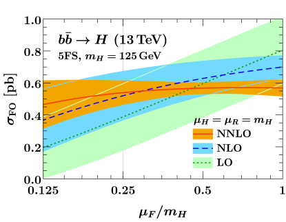
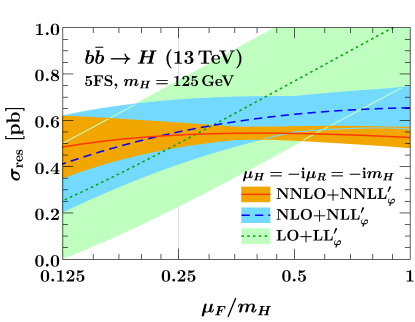
The perturbative series of the fixed-order cross section and its separation into $H_{q\bar{q}}^{S}$ and $R$ are given by

$$\sigma_{\mathrm{FO}}(\mu_{R}=m_{H},\mu_{F}=m_{H}/4) =(1+0.342+0.050)\times 0.387\,\mathrm{pb}\,,$$

$$H_{q\bar{q}}^{S}(m_{H}^{2},\mu_{H}=m_{H}) =\,\,1+0.227+0.054\,,$$

$$R(\mu_{R}=m_{H},\mu_{F}=m_{H}/4) =(1+0.115-0.031)\times 0.387\,\mathrm{pb}\,.$$ (42)

Although the perturbative corrections to the cross section are more moderate than for $gg\to H$, they are still clearly driven by the hard function, while the corrections to the remainder at $\mu_{F}=m_{H}/4$ are relatively small. The hard function itself shows a markedly improved convergence when evaluated at $\mu_{H}=-\mathrm{i}m_{H}$. Up to N³LO, we have

$$H_{q\bar{q}}^{S}(m_{H}^{2},\mu_{H}=m_{H}) =1+0.22742+0.05447+0.00507\,,$$

$$H_{q\bar{q}}^{S}(m_{H}^{2},\mu_{H}=-\mathrm{i}m_{H}) =1-0.00807+0.01202+0.00237\,,$$ (43)

showing that the corrections at real scales $\mu_{H}=m_{H}$ are mostly due to the timelike logarithms, which are eliminated at $\mu_{H}=-\mathrm{i}m_{H}$.

The resummed results are shown in the right panel of fig. 7, again as a function of the central choice for $\kappa_{F}$. From the above observations, we expect the resummed results to have an improved convergence at $\mu_{F}=m_{H}/4$. This is clearly seen, as the resummed predictions at the different orders roughly intersect at $\mu_{F}=m_{H}/4$, with the corrections beyond LO+$\text{LL}^{\prime}_{\varphi}$ amounting to less than $10\%$. The explicit numerical results at each order including a breakdown of the perturbative uncertainties are collected in table 3.

Note that the remainder $R$ carries the full $\mu_{F}$ dependence of the cross section. Evaluating it at $\kappa_{F}=1$, corresponding to $\mu_{F}=m_{H}$, its corrections are substantially larger than at $\mu_{F}=m_{H}/4$,

$$R(\mu_{R}=\mu_{F}=m_{H})=\sigma^{(0)}(\mu_{R}=\mu_{F}=m_{H})\times(1-0.359-0.136)\,.$$ (44)

We also checked that in the considered range of $\mu_{F}$ the perturbative coefficients of the remainder are indeed minimized around $\mu_{F}=m_{H}/4$. This explains why the resummed results in fig. 7 do not improve the fixed-order results above $\kappa_{F}=1/4$, since there the cross section becomes dominated by large negative corrections to the remainder and is also affected by accidental numerical cancellations between $H$ and $R$. Hence, the central choice $\kappa_{F}=1/4$ is also quite optimal from this point of view, as it leads to a clear “division of labor” between the remainder and the hard function in capturing the perturbative corrections to $b\bar{b}\rightarrow H$: By evaluating the former at an appropriate $\mu_{F}$ the collinear logarithms arising from initial-state $g\to b\bar{b}$ splittings are resummed into the $b$-quark PDFs, while the latter captures the hard virtual contributions to the $b\bar{b}H$ vertex, the bulk of which are enhanced at timelike kinematics and are resummed by setting $\mu_{H}=-\mathrm{i}m_{H}$.

The resummation also reduces the fixed-order uncertainty $\Delta_{\mu}$ by reducing the $\mu_{\mathrm{FO}}$ dependence and by eliminating large cross terms, which can also reduce the impact of the large $\mu_{F}$ dependence from lower-order contributions. This is seen in the slightly reduced $\mu_{F}$ dependence in fig. 7 at NLO+$\text{NLL}^{\prime}_{\varphi}$ and NNLO+$\text{NNLL}^{\prime}_{\varphi}$ compared to their fixed-order counterparts. However, the reduction of $\Delta_{\mu}$ is not nearly as dramatic as for $gg\to H$, because the $\mu_{F}$ dependence plays a much bigger role here. (In principle, the $\mu_{F}$ dependence and resulting uncertainties can be reduced further by reorganizing the perturbative series as discussed in ref. Bonvini:2015pxa , which is however beyond our scope here.) In table 3 we also include the $\Delta_{b}$ uncertainty from the low-scale $b$-quark PDF. (The parametric uncertainty in $m_{b}$ is much smaller than $\Delta_{b}$ and not considered.) The resummation uncertainty $\Delta_{\varphi}$ is completely negligible compared to $\Delta_{\mu}$, thanks to the very stable resummed hard function.

$\sigma\,[\!\,\mathrm{pb}]$ for $b\bar{b}\to H$, $E_{\mathrm{cm}}=13\,\mathrm{TeV}$, $m_{H}=125\,\mathrm{GeV}$
$n$	$\sigma_{\mathrm{FO}}$ at N$n$LO	$\sigma_{\mathrm{res}}$ at N$n$LO+$\text{N\textsuperscript{$n$}LL}^{\prime}_{\varphi}$
$0$	$0.387\!\pm\!0.208_{\mu}\!\pm\!0.020_{b}\,(54\%)$	$0.500\!\pm\!0.269_{\mu}\!\pm\!0.026_{b}\!\pm\!0.033_{\varphi}\,(54\%)$
$1$	$0.520\!\pm\!0.153_{\mu}\!\pm\!0.027_{b}\,(30\%)$	$0.550\!\pm\!0.138_{\mu}\!\pm\!0.028_{b}\!\pm\!0.006_{\varphi}\,(26\%)$
$2$	$0.539\!\pm\!0.074_{\mu}\!\pm\!0.028_{b}\,(15\%)$	$0.537\!\pm\!0.052_{\mu}\!\pm\!0.028_{b}\!\pm\!0.002_{\varphi}\,(11\%)$

Table 3: Total $b\bar{b}\rightarrow H$ cross section at $m_{H}=125\,\mathrm{GeV}$ at the LHC with $E_{\mathrm{cm}}=13\,\mathrm{TeV}$. The central scales are $\mu_{\mathrm{FO}}=m_{H}$, $\kappa_{F}=1/4$, $\mu_{b}=m_{b}$. The percent uncertainties correspond to the quadratic sum of all uncertainties.

Overall, we find that the NNLO and NNLO+$\text{NNLL}^{\prime}_{\varphi}$ results are very similar, which is reassuring, and that the resummation of timelike logarithms provides a useful tool to accelerate the convergence of the $b\bar{b}\rightarrow H$ cross section and to reduce its perturbative uncertainties.

4.2 Drell-Yan rapidity spectrum

As final example we consider the rapidity spectrum of the Drell-Yan process, $pp\rightarrow Z/\gamma^{\ast}\rightarrow\ell^{+}\ell^{-}$, which is known to NNLO Anastasiou:2003yy ; Anastasiou:2003ds ; Melnikov:2006di ; Melnikov:2006kv ; Catani:2009sm , and at N³LO in the threshold limit Ravindran:2006bu ; Ravindran:2007sv ; Ahmed:2014uya . (For the inclusion of threshold resummation effects see e.g. refs. Sterman:1986aj ; Catani:1989ne ; Forte:2002ni ; Idilbi:2005ky ; Mukherjee:2006uu ; Bolzoni:2006ky ; Becher:2007ty .) The necessary quark vector form factor is known to three loops Kramer:1986sg ; Matsuura:1987wt ; Matsuura:1988sm ; Gehrmann:2005pd ; Moch:2005tm ; Moch:2005id ; Baikov:2009bg ; Lee:2010cga ; Gehrmann:2010ue . The corresponding hard matching coefficient $C_{q\bar{q}}^{V}$ for the quark vector current to N³LO was obtained in refs. Abbate:2010xh ; Gehrmann:2010ue . We also need the matching coefficient $C_{q\bar{q}}^{A}$ for the axial-vector current, which is equal to the vector coefficient up to singlet corrections that start entering at $\mathcal{O}(\alpha_{s}^{2})$ Stewart:2009yx . At NNLO the axial-vector coefficient receives a nonvanishing singlet contribution from the axial-vector anomaly due to the large bottom-top mass splitting, but these contributions have been found to be small at cross section level Dicus:1985wx ; Hamberg:1990np . Since they are also not implemented in the program Vrap 0.9 Anastasiou:2003ds , which we use for our fixed-order predictions, we set $C_{q\bar{q}}^{A}=C_{q\bar{q}}^{V}$, dropping any singlet terms, and take $H_{q\bar{q}}\equiv\lvert C_{q\bar{q}}^{V}\rvert^{2}$ for our analysis. The RGE in either case is identical, since the axially anomalous terms are nonlogarithmic, and reads

$$\mu\frac{\mathrm{d}}{\mathrm{d}\mu}C_{q\bar{q}}^{V,A}(Q^{2},\mu) =\gamma_{q\bar{q}}^{V,A}(Q,\mu)\,C_{q\bar{q}}^{V,A}(Q^{2},\mu)\,,$$

$$\gamma_{q\bar{q}}^{V,A}(Q^{2},\mu) =\Gamma^{q}_{\mathrm{cusp}}\bigl{[}\alpha_{s}(\mu)\bigr{]}\ln\frac{-Q^{2}-\mathrm{i}0}{\mu^{2}}+2\gamma_{C}^{q}\bigl{[}\alpha_{s}(\mu)\bigr{]}\,.$$ (45)

We consider the double differential cross section $\mathrm{d}^{2}\sigma/\mathrm{d}Y\,\mathrm{d}Q$, where $Y$ and $Q$ are the rapidity and invariant mass of the produced lepton pair, and for simplicity focus on the $Z$ pole, $Q=m_{Z}$. Note that perturbative corrections to the quark current can only have a weak logarithmic dependence on $Q$, so our observations also hold away from the $Z$ pole. We obtain the rapidity distribution from Vrap 0.9 Anastasiou:2003ds , taking into account $V=Z,\gamma^{\ast}$ and their interference terms.

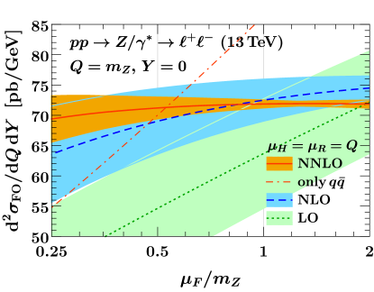
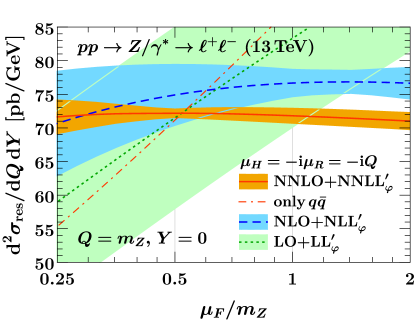
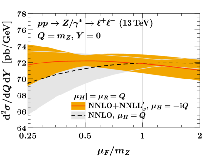
As for bottom-quark fusion, we can expect that for Drell-Yan the choice of $\mu_{F}$ will be important to improve the predictions by minimizing the perturbative corrections to the remainder. We first consider the rapidity spectrum at fixed $Y=0$. (Alternatively, one could integrate over rapidity, which yields similar conclusions.) Figure 8 shows the dependence on the factorization scale $\mu_{F}$ at fixed order (top left panel) and including the resummation of timelike logarithms in the quark form factor (top right panel), always using $\mu_{\mathrm{FO}}=\mu_{R}=m_{Z}$. In the bottom panel of fig. 8 we directly compare the NNLO (gray) and NNLO+$\text{NNLL}^{\prime}_{\varphi}$ (orange) results. The fixed-order results show the best convergence around $\mu_{F}=m_{Z}$, which is the typical choice adopted for Drell-Yan. In contrast, the resummed results clearly favor lower values of $\mu_{F}$. We therefore take $\mu_{F}=m_{Z}/2$ as our central choice, as in this region the lower-order uncertainties provide the best coverage of the higher-order results, while at the same time the $\mu_{F}$ dependence at the highest order is the most stable. (In principle, one might even consider going as low as $\mu_{F}\approx m_{Z}/4$ close to where the NLO+$\text{NLL}^{\prime}_{\varphi}$ and NNLO+$\text{NNLL}^{\prime}_{\varphi}$ central values coincide. However, the $\mu_{F}$ dependence is much larger there, and we also prefer to stay within a factor of two of the canonical value $\mu_{F}=m_{Z}$.) The dot-dashed line in fig. 8 shows the results at the highest order only including the $q\bar{q}$-initiated contributions. At $\mu_{F}=m_{Z}/2$, the cross section is dominated by the $q\bar{q}$ contribution, while at $\mu_{F}=m_{Z}$ the total NNLO corrections are small only due to substantial cancellations between the $q\bar{q}$ and remaining channels. This supports our central choice of $\mu_{F}=m_{Z}/2$ in the resummed results as the quark form factor is associated primarily with the $q\bar{q}$ channel. The explicit results at $Y=0$ are given in table 4, including a breakdown of the uncertainties.

Figure 8: Double-differential cross section $\mathrm{d}^{2}\sigma/\mathrm{d}Y\,\mathrm{d}Q$ for $pp\to Z/\gamma^{\ast}\to\ell^{+}\ell^{-}$ at $Q=m_{Z}$ and $Y=0$ and for $\mu_{\mathrm{FO}}=\mu_{R}=m_{Z}$ as a function of the central choice for $\kappa_{F}=\mu_{F}/m_{Z}$. The fixed-order results are shown on the left and the resummed results on the right. For illustration, the dot-dashed line shows the contribution from the $q\bar{q}$ channel at the highest order. In the bottom panel, the highest-order results at NNLO and NNLO+$\text{NNLL}^{\prime}_{\varphi}$ are directly compared with a further zoomed-in $y$-axis. The uncertainty bands show $\Delta_{\mu}$ (fixed order) and $\Delta_{\mu}\oplus\Delta_{\varphi}$ (resummed).

$\mathrm{d}^{2}\sigma/\mathrm{d}Y\,\mathrm{d}Q\,[\!\,\mathrm{pb}/\!\,\mathrm{GeV}]$ for $pp\to Z/\gamma^{\ast}\to\ell^{+}\ell^{-}$, $E_{\mathrm{cm}}=13\,\mathrm{TeV}$, $Q=m_{Z}$, $Y=0$
	$\mathrm{d}\sigma_{\mathrm{FO}}$ at N$n$LO		$\mathrm{d}\sigma_{\mathrm{res}}$ at N$n$LO+$\text{N\textsuperscript{$n$}LL}^{\prime}_{\varphi}$
$n$	$\mu_{F}=m_{Z}$	$\mu_{F}=m_{Z}/2$	$\mu_{F}=m_{Z}/2$
$0$	$63.7\!\pm\!9.1_{\mu}\,(14\%)$	$54.6\!\pm\!9.6_{\mu}\,(17\%)$	$71.5\!\pm\!12.6_{\mu}\!\pm\!5.0_{\varphi}\,(19\%)$
$1$	$72.5\!\pm\!3.5_{\mu}\,(4.8\%)$	$69.0\!\pm\!5.4_{\mu}\,(7.9\%)$	$74.9\!\pm\!4.2_{\mu}\!\pm\!1.6_{\varphi}\,(6.1\%)$
$2$	$71.9\!\pm\!0.7_{\mu}\,(0.9\%)$	$71.2\!\pm\!1.8_{\mu}\,(2.5\%)$	$72.2\!\pm\!0.6_{\mu}\!\pm\!0.2_{\varphi}\,(0.9\%)$

Table 4: Cross section for $pp\to Z/\gamma^{\ast}\to\ell^{+}\ell^{-}$ at $Q=m_{Z}$ and $Y=0$ at the LHC with $E_{\mathrm{cm}}=13\,\mathrm{TeV}$. The central scale is always $\mu_{\mathrm{FO}}=\mu_{R}=m_{Z}$. The percent uncertainties for the resummed results correspond to the total uncertainty $\Delta_{\mu}\oplus\Delta_{\varphi}$.

The perturbative series of the fixed-order cross section at $Q=m_{Z}$ and $Y=0$ and its decomposition into hard function $H_{q\bar{q}}$ and remainder $R$ at $\mu_{F}=m_{Z}$ and $\mu_{F}=m_{Z}/2$ is given by

$$\mathrm{d}^{2}\sigma_{\mathrm{FO}}(\mu_{R}=m_{Z},\mu_{F}=m_{Z}) =(1+0.138-0.010)\times 63.7\,\mathrm{pb}/\!\,\mathrm{GeV}\,,$$

$$H_{q\bar{q}}(m_{Z}^{2},\mu_{H}=m_{Z}) =\,\,1+0.088+0.0317\,,$$

$$R(\mu_{R}=m_{Z},\mu_{F}=m_{Z}) =(1+0.050-0.046)\times 63.7\,\mathrm{pb}/\!\,\mathrm{GeV}\,,$$

$$\mathrm{d}^{2}\sigma_{\mathrm{FO}}(\mu_{R}=m_{Z},\mu_{F}=m_{Z}/2) =(1+0.263+0.040)\times 54.6\,\mathrm{pb}/\!\,\mathrm{GeV}\,,$$

$$H_{q\bar{q}}(m_{Z}^{2},\mu_{H}=m_{Z}) =\,\,1+0.088+0.0317\,,$$

$$R(\mu_{R}=m_{Z},\mu_{F}=m_{Z}/2) =(1+0.175-0.007)\times 54.6\,\mathrm{pb}/\!\,\mathrm{GeV}\,.$$ (46)

The corrections to the fixed-order cross section are smaller at $\mu_{F}=m_{Z}$. However, its small NNLO contribution stems from a numerical cancellation between $H_{q\bar{q}}$ and $R$, and as discussed in sec. 2, there is a priori no reason to expect that this continues to happen at higher orders. Also, the NLO and NNLO contributions for $R$ are of the same size, indicating that the NLO contribution is artificially small or the NNLO contribution unusually large or a mixture of both. For $\mu_{F}=m_{Z}/2$, the NNLO contribution to $R$ is very small and the NNLO contribution to the cross section primarily comes from $H_{q\bar{q}}$. It will be interesting to see how this pattern continues at N³LO.

The hard function itself shows again a notably improved convergence at $\mu_{H}=-\mathrm{i}m_{Z}$ compared to $\mu_{H}=m_{Z}$,

$$H_{q\bar{q}}^{V}(m_{Z},\mu_{H}=m_{Z}) =1+0.08801+0.03169+0.00745\,,$$

$$H_{q\bar{q}}^{V}(m_{Z},\mu_{H}=-\mathrm{i}m_{Z}) =1-0.15048-0.00126-0.00101\,.$$ (47)

As for $b\bar{b}H$, the improvement is not as dramatic as for gluon fusion due to the reduced color factor for quarks vs. gluons. Nevertheless, by eliminating the timelike logarithms in $H_{q\bar{q}}$, the higher-order contributions are substantially reduced, except that the NLO contribution actually gets larger (in contrast to $b\bar{b}H$). The reason for this is an accidental numerical cancellation in the one-loop matching coefficient

$$C_{q\bar{q}}^{V}(Q,\mu)=1+\frac{\alpha_{s}(\mu)}{4\pi}C_{F}\left[-\ln^{2}\left(\frac{-Q^{2}-\mathrm{i}0}{\mu^{2}}\right)+3\ln\left(\frac{-Q^{2}-\mathrm{i}0}{\mu^{2}}\right)-8+\frac{\pi^{2}}{6}\right]+{\mathcal{O}}\Bigl{(}\alpha_{s}^{2}(\mu)\Bigr{)}\,,$$ (48)

where the rather large nonlogarithmic constant term of $-8+\pi^{2}/6$ partially cancels the $-\ln^{2}(-1)=\pi^{2}$ when $H_{q\bar{q}}$ is evaluated at $\mu_{H}=m_{Z}$. As discussed in sec. 2, the separation of the nonlogarithmic constant terms between $H$ and $R$ amounts to a scheme choice and only their sum is ultimately relevant. Hence, this large NLO constant term is a scheme-dependent artifact and in fact cancels most of the equally large NLO contribution in $R(\mu_{F}=m_{Z}/2)$. This also means that the $+0.263$ NLO contribution in the cross section at $\mu_{F}=m_{Z}/2$ in eq. (4.2) does in fact primarily come from the NLO timelike logarithm in $H_{q\bar{q}}$, which gives a contribution of $+0.247$ to it, even though this is not immediately obvious from eq. (4.2). This explains the much improved convergence of the resummed results at $\mu_{F}=m_{Z}/2$ compared to the fixed-order results at the same scale.

It was already noted in ref. Magnea:1990zb that the constant terms in $C_{q\bar{q}}^{V}$ are scheme dependent and hence not physical, unlike the ratio of form factors. Since the constant terms in $H$ and $R$ are evaluated at different scales, there is a residual scheme dependence, which is analogous to a scale choice in that it affects the numerical results but is formally of higher order [see eq. (13)]. To check this, we can consider an alternative renormalization scheme for the Wilson coefficient $\tilde{C}_{q\bar{q}}^{V}$, for which all constant terms exactly vanish. That is, the corresponding hard function solely consists of timelike logarithms, $\tilde{H}_{q\bar{q}}^{V}(m_{Z}^{2},\mu_{H}=m_{Z})=1+0.247+0.073+0.013$, while $\tilde{H}_{q\bar{q}}^{V}(m_{Z}^{2},\mu_{H}=-\mathrm{i}m_{Z})=1+0+0+0$. Hence, the constant terms are moved entirely into the remainder. In this scheme, the resummed result at NNLO+$\text{NNLL}^{\prime}_{\varphi}$ is $\mathrm{d}^{2}{\tilde{\sigma}}_{\mathrm{res}}(Y=0,Q=m_{Z},\mu_{R}=m_{Z},\mu_{F}=m_{Z}/2)=(71.4\!\pm\!0.7_{\mu}\!\pm\!0.2_{\varphi})\,\mathrm{pb}/\!\,\mathrm{GeV}\,(1.0\%)$. Compared to the last line of table 4, the difference of $\pm 0.8\,\mathrm{pb}$ is of the same size as the uncertainties and thus of the typical size we expect for an $\mathcal{O}(\alpha_{s}^{3})$ effect.

Figure 9: The perturbative remainder $R(Y)$ for $pp\to Z/\gamma^{\ast}\to\ell^{+}\ell^{-}$, normalized to $\sigma^{(0)}(Y)\equiv\mathrm{d}^{2}\sigma^{(0)}/\mathrm{d}Q\,\mathrm{d}Y$ at $Q=m_{Z}$ for $\mu_{F}=m_{Z}$ (left) and $\mu_{F}=m_{Z}/2$ (right). The dot-dashed line shows the result including only the $q\bar{q}$ channel.

Figure 10: Rapidity spectrum for $pp\to Z/\gamma^{\ast}\to\ell^{+}\ell^{-}$ at $Q=m_{Z}$. The fixed-order results are shown for $Y<0$ and the resummed results for $Y>0$. For the central scale we use $\mu_{\mathrm{FO}}=m_{Z}$ in both cases, while $\kappa_{F}=1$ (fixed order) and $\kappa_{F}=1/2$ (resummed). The uncertainty bands indicate $\Delta_{\mu}$ (fixed order) and $\Delta_{\mu}\oplus\Delta_{\varphi}$ (resummed).

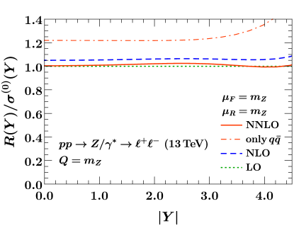
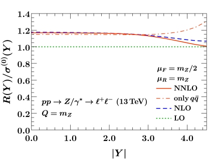
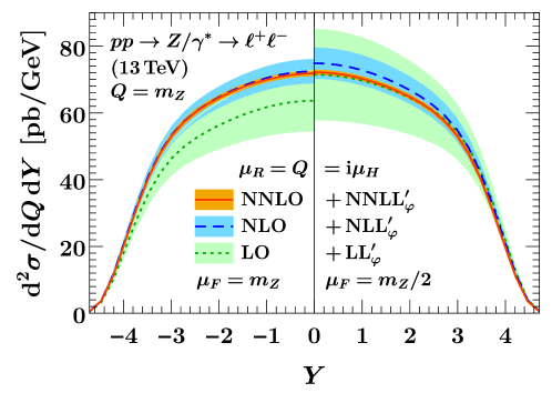
We now discuss the effect of the resummation on the rapidity spectrum. In fig. 9, we show the remainder $R(Y)$ normalized to the Born cross section as a function of $Y$ for $\mu_{F}=m_{Z}$ (left) and $\mu_{F}=m_{Z}/2$ (right). The behavior discussed for $Y=0$ above is similar throughout most of the spectrum. For $\mu_{F}=m_{Z}$, the NNLO corrections are comparably large and of the same size and opposite sign as the NLO contributions, while the NNLO corrections are almost negligible at $\mu_{F}=m_{Z}/2$ over most of the rapidity range. We see again that at $\mu_{F}=m_{Z}$ the NNLO corrections involve substantial cancellations between the $q\bar{q}$ and non-$q\bar{q}$ channels, which individually are very large. In contrast, at $\mu_{F}=m_{Z}/2$ also the individual corrections to the remainder are very small, again supporting this central choice when including the resummation. (A large part of the rapidity-independent constant shift at NLO will again be canceled by the constant term in $H_{q\bar{q}}$.) In fig. 10, we compare the rapidity spectrum at $Q=m_{Z}$, where the fixed-order calculation at its optimal $\mu_{F}=m_{Z}$ is shown for $Y<0$ and the resummed result at $\mu_{F}=m_{Z}/2$ for $Y>0$.

Overall, we find that the NNLO and NNLO+$\text{NNLL}^{\prime}_{\varphi}$ predictions provide very similar results. On the one hand, this is reassuring, as it shows that the good convergence of the fixed-order series is not spoiled by the resummation. On the other hand, given the extreme reduction of the perturbative uncertainties in the fixed-order results at the conventional choice of $\mu_{F}=m_{Z}$ by a factor of five when going from NLO to NNLO and the substantially larger uncertainties at $\mu_{F}=m_{Z}/2$, one might perhaps be worried that the fixed-order uncertainties are somewhat underestimated, in part due to the accidentally small NNLO contribution. In this respect, the resummed results provide a useful confirmation and increased confidence in the very small perturbative uncertainties in the Drell-Yan predictions.

5 Conclusion

We have investigated in detail the resummation of timelike logarithms $\ln^{2}(-1)=-\pi^{2}$ that arise to all orders in perturbation theory and are an important source of perturbative corrections in $s$-channel color-singlet production processes, which involve a timelike hard momentum transfer. These logarithms can be resummed to all orders using the RG evolution of the corresponding quark or gluon form factors from spacelike to timelike scales.

We have shown how to incorporate the resummed form factor in a completely straightforward manner into predictions for generic inclusive cross sections with arbitrary dependence or cuts on the Born kinematics. We have verified that this does not spoil the perturbative series in all considered cases. We have also discussed the assessment of the uncertainties intrinsic to the resummation.

We first revisited the resummation for the total gluon-fusion cross section, for which it has been discussed before, considering both the production of a generic scalar as well as the SM Higgs boson in the $m_{t}\to\infty$ limit up to N³LO+$\text{N\textsuperscript{3}LL}^{\prime}_{\varphi}$. For the latter we have also shown how to incorporate quark-mass and electroweak effects. We confirm that the resummation significantly improves the perturbative series, and find that it reduces the perturbative uncertainties at the highest orders by about a factor of two.

For the Higgs rapidity spectrum as well as the cross section with a cut on the Higgs rapidity we obtain results at NNLO+$\text{NNLL}^{\prime}_{\varphi}$, which provide the currently most precise predictions with central values close to what might be expected at N³LO, and perturbative uncertainties of $\sim 6\%$, which are almost a factor of two smaller than at NNLO. Once N³LO results for the rapidity dependence become available, we project that the corresponding resummation at N³LO+$\text{N\textsuperscript{3}LL}^{\prime}_{\varphi}$ will provide a similar improvement.

We also studied the resummation of timelike logarithms for quark-induced processes, namely Higgs production through bottom-quark annihilation and the Drell-Yan rapidity spectrum. For the former, the resummation provides a small improvement in the perturbative convergence and resulting uncertainties. For Drell-Yan production, the resummation provides no clear improvement but also no worsening of the predictions, due to the already fast convergence of the fixed-order perturbative series. In this case it provides a useful confirmation of the very small residual perturbative uncertainties.

We conclude that utilizing the resummed timelike quark and gluon form factors is viable and beneficial for obtaining precise and reliable predictions for $s$-channel color-singlet production processes.

Appendix A Perturbative ingredients

A.1 Master formula for hard Wilson coefficients to three loops

The hard matching coefficients $C$ satisfy an RGE of the form

$$\mu\frac{\mathrm{d}}{\mathrm{d}\mu}C(q^{2},\mu)=\Bigl{\{}\Gamma_{\mathrm{cusp}}[\alpha_{s}(\mu)]\ln\frac{-q^{2}-\mathrm{i}0}{\mu^{2}}+\gamma[\alpha_{s}(\mu)]\Bigr{\}}C(q^{2},\mu)\,,$$ (49)

which allows us to completely predict the logarithmic structure in terms of the cusp and noncusp anomalous dimension coefficients. We write the perturbative expansion of the hard coefficient as

$$C(q^{2},\mu)=\sum_{n=0}^{\infty}C^{(n)}(L)\biggl{[}\frac{\alpha_{s}(\mu)}{4\pi}\biggr{]}^{n}\,,\qquad L=\ln\frac{-q^{2}-\mathrm{i}0}{\mu^{2}}\,,\qquad C_{n}=C^{(n)}(0)\,.$$ (50)

Normalizing $C$ such that the tree-level result is $C_{0}=1$, the perturbative solution of eq. (49) to N³LO is given by

$$C^{(0)} =1\,,$$

$$C^{(1)}(L) =-\frac{L^{2}}{4}\Gamma_{0}-\frac{L}{2}\gamma_{0}+C_{1}\,,$$

$$C^{(2)}(L) =\frac{L^{4}}{32}\Gamma_{0}^{2}+\frac{L^{3}}{24}\Gamma_{0}(2\beta_{0}+3\gamma_{0})+\frac{L^{2}}{8}(2\beta_{0}\gamma_{0}+\gamma_{0}^{2}-2C_{1}\Gamma_{0}-2\Gamma_{1})$$

$$\quad-\frac{L}{2}(2C_{1}\beta_{0}+C_{1}\gamma_{0}+\gamma_{1})+C_{2}\,,$$

$$C^{(3)}(L) =-\frac{L^{6}}{384}\Gamma_{0}^{3}-\frac{L^{5}}{192}\Gamma_{0}^{2}(4\beta_{0}+3\gamma_{0})+\frac{L^{4}}{96}\Gamma_{0}\bigl{(}-4\beta_{0}^{2}-10\beta_{0}\gamma_{0}-3\gamma_{0}^{2}+3C_{1}\Gamma_{0}+6\Gamma_{1}\bigr{)}$$

$$\quad+\frac{L^{3}}{48}\Bigl{[}-8\beta_{0}^{2}\gamma_{0}-6\beta_{0}\gamma_{0}^{2}-\gamma_{0}^{3}+\Gamma_{0}(16C_{1}\beta_{0}+6C_{1}\gamma_{0}+6\gamma_{1}+4\beta_{1})+\Gamma_{1}(8\beta_{0}+6\gamma_{0})\Bigr{]}$$

$$\quad+\frac{L^{2}}{8}\Bigl{[}C_{1}(8\beta_{0}^{2}+6\beta_{0}\gamma_{0}+\gamma_{0}^{2}-2\Gamma_{1})+2\beta_{1}\gamma_{0}+4\beta_{0}\gamma_{1}+2\gamma_{0}\gamma_{1}-2C_{2}\Gamma_{0}-2\Gamma_{2}\Bigr{]}$$

$$\quad-\frac{L}{2}\bigl{(}4C_{2}\beta_{0}+2C_{1}\beta_{1}+C_{2}\gamma_{0}+C_{1}\gamma_{1}+\gamma_{2}\bigr{)}+C_{3}\,.$$ (51)

Here, $\beta_{n}$ are the beta-function coefficients, $\Gamma_{n}\equiv\Gamma_{n}^{i}$ the appropriate quark or gluon cusp anomalous dimensions coefficients, and $\gamma_{n}$ are the coefficients of the total noncusp anomalous dimension $\gamma$ in eq. (49) as appropriate for the hard coefficient of interest. All required anomalous dimension coefficients are given below in appendix A.2. The results for the nonlogarithmic constant terms $C_{n}$ for the different Wilson coefficients are given below in appendix A.3

The full expression for the hard function is obtained by squaring $C$, accounting for cross terms. In the case of $H_{gg}^{t}$ defined in eq. (3.3) the product of $C_{t}\,C_{gg}$ is reexpanded.

A.2 Anomalous dimensions

We expand the $\beta$ function of QCD as

$$\mu\frac{\mathrm{d}\alpha_{s}(\mu)}{\mathrm{d}\mu}=\beta[\alpha_{s}(\mu)]\,,\qquad\beta(\alpha_{s})=-2\alpha_{s}\sum_{n=0}^{\infty}\beta_{n}\left(\frac{\alpha_{s}}{4\pi}\right)^{n+1}\,.$$ (52)

The coefficients up to four loops in the $\overline{\text{MS}}$ scheme are Tarasov:1980au ; Larin:1993tp ; vanRitbergen:1997va ; Czakon:2004bu

$$\beta_{0} =\frac{11}{3}\,C_{A}-\frac{4}{3}\,T_{F}\,n_{f}\,,$$

$$\beta_{1} =\frac{34}{3}\,C_{A}^{2}-\Bigl{(}\frac{20}{3}\,C_{A}\,+4C_{F}\Bigr{)}\,T_{F}\,n_{f}\,,$$ (53)

$$\beta_{2} =\frac{2857}{54}\,C_{A}^{3}+\Bigl{(}C_{F}^{2}-\frac{205}{18}\,C_{F}C_{A}-\frac{1415}{54}\,C_{A}^{2}\Bigr{)}\,2T_{F}\,n_{f}+\Bigl{(}\frac{11}{9}\,C_{F}+\frac{79}{54}\,C_{A}\Bigr{)}\,4T_{F}^{2}\,n_{f}^{2}\,,$$

$$\beta_{3} =\Bigl{(}\frac{149753}{6}+3564\zeta_{3}\Bigr{)}-\Bigl{(}\frac{1078361}{162}+\frac{6508}{27}\zeta_{3}\Bigr{)}n_{f}+\Bigl{(}\frac{50065}{162}+\frac{6472}{81}\zeta_{3}\Bigr{)}n_{f}^{2}+\frac{1093}{729}n_{f}^{3}\,,$$

where for $\beta_{3}$ we specified to $\mathrm{SU}(3)$ for brevity. Throughout our analysis, we consider $n_{f}=5$ active flavors.

The cusp and noncusp anomalous dimensions are expanded as

$$\Gamma^{i}_{\mathrm{cusp}}(\alpha_{s})=\sum_{n=0}^{\infty}\Gamma^{i}_{n}\Bigl{(}\frac{\alpha_{s}}{4\pi}\Bigr{)}^{n+1}\,,\qquad\gamma(\alpha_{s})=\sum_{n=0}^{\infty}\gamma_{n}\Bigl{(}\frac{\alpha_{s}}{4\pi}\Bigr{)}^{n+1}\,.$$ (54)

The coefficients of the $\overline{\mathrm{MS}}$ cusp anomalous dimension to three loops are Korchemsky:1987wg ; Moch:2004pa ; Vogt:2004mw

$$\Gamma^{q}_{n} =C_{F}\Gamma_{n}\,,\qquad\Gamma^{g}_{n}=C_{A}\Gamma_{n}\,,\qquad\text{(for $n=0,1,2$)}\,,$$

$$\Gamma_{0} =4\,,$$

$$\Gamma_{1} =4\Bigl{[}C_{A}\Bigl{(}\frac{67}{9}-\frac{\pi^{2}}{3}\Bigr{)}-\frac{20}{9}\,T_{F}\,n_{f}\Bigr{]}=\frac{4}{3}\bigl{[}(4-\pi^{2})C_{A}+5\beta_{0}\bigr{]}\,,$$

$$\Gamma_{2} =4\Bigl{[}C_{A}^{2}\Bigl{(}\frac{245}{6}-\frac{134\pi^{2}}{27}+\frac{11\pi^{4}}{45}+\frac{22\zeta_{3}}{3}\Bigr{)}+C_{A}\,T_{F}\,n_{f}\Bigl{(}-\frac{418}{27}+\frac{40\pi^{2}}{27}-\frac{56\zeta_{3}}{3}\Bigr{)}$$

$$\qquad+C_{F}\,T_{F}\,n_{f}\Bigl{(}-\frac{55}{3}+16\zeta_{3}\Bigr{)}-\frac{16}{27}\,T_{F}^{2}\,n_{f}^{2}\Bigr{]}\,.$$ (55)

The resummation at N³LL formally also requires the yet unknown four-loop coefficient $\Gamma_{3}^{i}$, which we estimate as usual by the Padé approximation

$$\Gamma^{i}_{3,\,\text{Pad{\'{e}}}}=\frac{(\Gamma^{i}_{2})^{2}}{\Gamma_{1}^{i}}\,,$$ (56)

and explicitly verify that a variation $\pm 200\%$ only affects the hard evolution kernel $U_{H}$ (and thus the resummed cross section) at the sub-permille level. We therefore neglect this source of theory uncertainty.

The gluon noncusp anomalous dimension $\gamma_{C}^{g}$ enters the RGE for the gluon-to-scalar matching coefficients $C_{gg}$ and $C_{gg}^{\prime}$ in eqs. (22) and (3.3). The coefficients in $\overline{\text{MS}}$ up to three loops are Moch:2005tm ; Idilbi:2005ni ; Idilbi:2006dg

$$\gamma_{C\,0}^{g} =-\beta_{0}\,,$$

$$\gamma_{C\,1}^{g} =C_{A}\biggl{[}C_{A}\Bigl{(}-\frac{59}{9}+2\zeta_{3}\Bigr{)}+\beta_{0}\Bigl{(}-\frac{19}{9}+\frac{\pi^{2}}{6}\Bigr{)}\biggr{]}-\beta_{1}\,,$$

$$\gamma_{C\,2}^{g} =\frac{C_{A}}{2}\biggl{[}C_{A}^{2}\Bigl{(}-\frac{60875}{162}+\frac{634\pi^{2}}{81}+\frac{8\pi^{4}}{5}+\frac{1972\zeta_{3}}{9}-\frac{40\pi^{2}\zeta_{3}}{9}-32\zeta_{5}\Bigr{)}$$

$$\qquad\quad+C_{A}\beta_{0}\Bigl{(}\frac{7649}{54}+\frac{134\pi^{2}}{81}-\frac{61\pi^{4}}{45}-\frac{500\zeta_{3}}{9}\Bigr{)}+\beta_{0}^{2}\Bigl{(}\frac{466}{81}+\frac{5\pi^{2}}{9}-\frac{28\zeta_{3}}{3}\Bigr{)}$$

$$\qquad\quad+\beta_{1}\Bigl{(}-\frac{1819}{54}+\frac{\pi^{2}}{3}+\frac{4\pi^{4}}{45}+\frac{152\zeta_{3}}{9}\Bigr{)}\biggr{]}-\beta_{2}\,.$$ (57)

The evolution of $C_{gg}^{t}$ in the one-step matching also requires the anomalous dimension $\gamma_{t}$ of the Wilson coefficient $C_{t}$ arising from integrating out the top quark. It is given by

$$\gamma_{t}(\alpha_{s})=\alpha_{s}^{2}\frac{\mathrm{d}}{\mathrm{d}\alpha_{s}}\frac{\beta(\alpha_{s})}{\alpha_{s}^{2}}\,,\qquad\gamma_{t\,n}=-2n\cdot\beta_{n}\,.$$ (58)

The quark noncusp anomalous dimension $\gamma_{C}^{q}$ enters the RG eqs. (4.1) and (45) for both quark-induced processes we consider. The coefficients in $\overline{\text{MS}}$ up to three loops are Moch:2005id ; Moch:2005tm ; Idilbi:2006dg ; Becher:2006mr

$$\gamma^{q}_{C\,0} =-3C_{F}\,,$$

$$\gamma^{q}_{C\,1} =-C_{F}\biggl{[}C_{A}\Bigl{(}\frac{41}{9}-26\zeta_{3}\Bigr{)}+C_{F}\Bigl{(}\frac{3}{2}-2\pi^{2}+24\zeta_{3}\Bigr{)}+\beta_{0}\Bigl{(}\frac{65}{18}+\frac{\pi^{2}}{2}\Bigr{)}\biggr{]}\,,$$

$$\gamma^{q}_{C\,2} =-C_{F}\biggl{[}C_{A}^{2}\Bigl{(}\frac{66167}{324}-\frac{686\pi^{2}}{81}-\frac{302\pi^{4}}{135}-\frac{782\zeta_{3}}{9}+\frac{44\pi^{2}\zeta_{3}}{9}+136\zeta_{5}\Bigr{)}$$

$$\qquad\qquad+C_{F}C_{A}\Bigl{(}\frac{151}{4}-\frac{205\pi^{2}}{9}-\frac{247\pi^{4}}{135}+\frac{844\zeta_{3}}{3}+\frac{8\pi^{2}\zeta_{3}}{3}+120\zeta_{5}\Bigr{)}$$

$$\qquad\qquad+C_{F}^{2}\Bigl{(}\frac{29}{2}+3\pi^{2}+\frac{8\pi^{4}}{5}+68\zeta_{3}-\frac{16\pi^{2}\zeta_{3}}{3}-240\zeta_{5}\Bigr{)}$$

$$\qquad\qquad+C_{A}\beta_{0}\Bigl{(}-\frac{10781}{108}+\frac{446\pi^{2}}{81}+\frac{449\pi^{4}}{270}-\frac{1166\zeta_{3}}{9}\Bigr{)}$$

$$\qquad\qquad+\beta_{1}\Bigl{(}\frac{2953}{108}-\frac{13\pi^{2}}{18}-\frac{7\pi^{4}}{27}+\frac{128\zeta_{3}}{9}\Bigr{)}+\beta_{0}^{2}\Bigl{(}-\frac{2417}{324}+\frac{5\pi^{2}}{6}+\frac{2\zeta_{3}}{3}\Bigr{)}\biggr{]}\,.$$ (59)

The evolution of $C_{q\bar{q}}^{S}$ also requires the anomalous dimension of the quark Yukawa coupling, which is equivalent to the quark mass anomalous dimension $\gamma_{m}$,

$$\mu\frac{\mathrm{d}}{\mathrm{d}\mu}y(\mu)=\gamma_{m}[\alpha_{s}(\mu)]\,y(\mu)\,.$$ (60)

It is known to five loops Tarrach:1980up ; Tarasov:1982gk ; Larin:1993tq ; Vermaseren:1997fq ; Chetyrkin:1997dh ; Baikov:2014qja ; Luthe:2016xec . For our main analysis at NNLL we only require the two-loop result, while the three-loop coefficient $\gamma_{m\,2}$ serves to verify our N³LO result for $C_{q\bar{q}}^{S}$. The results are

$$\gamma_{m\,0} =-6C_{F}\,,$$

$$\gamma_{m\,1} =-2C_{F}\Bigl{(}\frac{3}{2}\,C_{F}+\frac{97}{6}\,C_{A}-\frac{10}{3}\,T_{F}\,n_{f}\Bigr{)}\,,$$

$$\gamma_{m\,2} =-2C_{F}\biggl{[}\frac{11413}{108}\,C_{A}^{2}-\frac{129}{4}\,C_{F}C_{A}+\frac{129}{2}\,C_{F}^{2}+C_{A}\,T_{F}\,n_{f}\,\Bigl{(}-\frac{556}{27}-48\zeta_{3}\Bigr{)}$$

$$\qquad\qquad+C_{F}\,T_{F}\,n_{f}\,(-46+48\zeta_{3})-\frac{140}{27}T_{F}^{2}\,n_{f}^{2}\biggr{]}\,.$$ (61)

A.3 Constant terms to three loops

In the following, we provide the process-specific nonlogarithmic constant terms $C_{n}$ for the various hard matching coefficients. For $C_{gg}$, $C_{t}$, and $C_{q\bar{q}}^{V}$, we can collect the results from the literature. The result for $C_{q\bar{q}}^{S}$ we have extracted from the three-loop scalar quark form factor. By convention, we normalize all coefficients to unity at LO,

$$C_{gg\,0}=C_{t\,0}=C_{q\bar{q}\,0}^{V}=C_{gg\,0}^{S}=1\,.$$ (62)

Note that for all coefficients quoted here, we closely follow the notation from the original publications. For this reason, we set $T_{F}=1/2$ in the following results.

A.3.1 Gluon matching coefficient

The finite terms of $C_{gg}$ can be read off from the full result given in ref. Gehrmann:2010ue ,

$$C_{gg\,1} =C_{A}\,\zeta_{2}\,,$$

$$C_{gg\,2} =C_{A}^{2}\Bigl{(}\frac{5105}{162}-\frac{143}{9}\zeta_{3}+\frac{67}{6}\zeta_{2}+\frac{1}{2}\zeta_{2}^{2}\Bigr{)}+C_{A}\,n_{f}\Bigl{(}-\frac{916}{81}-\frac{46}{9}\zeta_{3}-\frac{5}{3}\zeta_{2}\Bigr{)}$$

$$\quad+C_{F}\,n_{f}\Bigl{(}-\frac{67}{6}+8\zeta_{3}\Bigr{)}\,,$$

$$C_{gg\,3} =C_{A}^{3}\Bigl{(}+\frac{29639273}{26244}-\frac{1939}{270}\zeta_{2}^{2}+\frac{2222}{9}\zeta_{5}+\frac{105617}{729}\zeta_{2}-\frac{24389}{1890}\zeta_{2}^{3}-\frac{152716}{243}\zeta_{3}$$

$$\qquad\quad-\frac{605}{9}\zeta_{2}\zeta_{3}-\frac{104}{9}\zeta_{3}^{2}\Bigr{)}$$

$$\quad+C_{A}^{2}\,n_{f}\Bigl{(}-\frac{3765007}{6561}+\frac{428}{9}\zeta_{5}-\frac{460}{81}\zeta_{3}-\frac{14189}{729}\zeta_{2}-\frac{82}{9}\zeta_{2}\zeta_{3}+\frac{73}{45}\zeta_{2}^{2}\Bigr{)}$$

$$\quad+C_{A}C_{F}\,n_{f}\Bigl{(}-\frac{341219}{972}+\frac{608}{9}\zeta_{5}+\frac{14564}{81}\zeta_{3}-\frac{68}{9}\zeta_{2}+\frac{64}{3}\zeta_{2}\zeta_{3}-\frac{64}{45}\zeta_{2}^{2}\Bigr{)}$$

$$\quad+C_{F}^{2}\,n_{f}\,\Bigl{(}\frac{304}{9}-160\zeta_{5}+\frac{296}{3}\zeta_{3}\Bigr{)}$$

$$\quad+C_{A}\,n_{f}^{2}\Bigl{(}\frac{611401}{13122}+\frac{4576}{243}\zeta_{3}+\frac{4}{9}\zeta_{2}+\frac{4}{27}\zeta_{2}^{2}\Bigr{)}$$

$$\quad+C_{F}\,n_{f}^{2}\Bigl{(}\frac{4481}{81}-\frac{112}{3}\zeta_{3}-\frac{20}{9}\zeta_{2}-\frac{16}{45}\zeta_{2}^{2}\Bigr{)}\,.$$ (63)

A.3.2 $C_{t}$ coefficient for Higgs production in the EFT limit

The general expression for $C_{t}(m_{t},\mu)$ up to $\mathcal{O}(\alpha_{s}^{3})$ is given by

$$C_{t}(m_{t},\mu) =1+C_{t\,1}\frac{\alpha_{s}(\mu)}{4\pi}+\biggl{[}(\beta_{1}-\beta_{0}C_{t\,1})\ln\frac{m_{t}^{2}}{\mu^{2}}+C_{t\,2}\biggr{]}\frac{\alpha_{s}^{2}(\mu)}{(4\pi)^{2}}$$

$$\quad+\biggl{[}-\beta_{0}(\beta_{1}-\beta_{0}C_{t\,1})\ln^{2}\frac{m_{t}^{2}}{\mu^{2}}+2(\beta_{2}-\beta_{0}C_{t\,2})\ln\frac{m_{t}^{2}}{\mu^{2}}+C_{t\,3}\biggr{]}\frac{\alpha_{s}^{3}(\mu)}{(4\pi)^{3}}\,.$$ (64)

The constant terms are given by

$$C_{t\,1} =5C_{A}-3C_{F}\,,$$

$$C_{t\,2} =\frac{91}{6}C_{A}^{2}-\frac{100}{3}C_{A}C_{F}+\frac{27}{2}C_{F}^{2}+C_{A}\Bigl{(}\frac{47}{12}\beta_{0}-\frac{5}{6}T_{F}\Bigr{)}-C_{F}T_{F}\Bigl{(}\frac{4}{3}+5n_{f}\Bigr{)}\,,$$

$$C_{t\,3} =-\frac{2761331}{648}+\frac{897943}{144}\zeta_{3}+n_{f}\Bigl{(}\frac{58723}{324}-\frac{110779}{216}\zeta_{3}\Bigr{)}-n_{f}^{2}\,\frac{6865}{486}\,,$$ (65)

where $C_{t\,3}$ is taken from ref. Anastasiou:2016cez , where all color factors are already evaluated for $N_{c}=3$.

The dependence of $H_{gg}^{t}$ on $\rho=m_{H}^{2}/(4m_{t}^{2})$ at NLO is given by Berger:2010xi

$$F_{1}(\rho) =C_{A}\Bigl{(}5-\frac{38}{45}\,\rho-\frac{1289}{4725}\,\rho^{2}-\frac{155}{1134}\,\rho^{3}-\frac{5385047}{65488500}\,\rho^{4}\Bigr{)}$$

$$\quad+C_{F}\Bigl{(}-3+\frac{307}{90}\,\rho+\frac{25813}{18900}\,\rho^{2}+\frac{3055907}{3969000}\,\rho^{3}+\frac{659504801}{1309770000}\,\rho^{4}\Bigr{)}+\mathcal{O}(\rho^{5})\,,$$ (66)

where $F_{1}(0)=C_{t\,1}$. The exact $\rho$ dependence of $F_{1}(\rho)$ in terms of harmonic polylogarithms is known Harlander:2005rq ; Anastasiou:2006hc ; Aglietti:2006tp . We use the results expanded in $\rho$, which are completely sufficient for practical purposes because the corrections are small and the expansion in $\rho\simeq 0.13$ converges very quickly.

A.3.3 Quark vector-current matching coefficient

The finite terms of $C_{q\bar{q}}^{V}$ to three loops can be read off from ref. Gehrmann:2010ue ,

$$C^{V}_{q\bar{q}\,1} =C_{F}(-8+\zeta_{2})\,,$$

$$C^{V}_{q\bar{q}\,2} =C_{F}\biggl{[}C_{A}\Bigl{(}-\frac{51157}{648}+\frac{313}{9}\zeta_{3}-\frac{337}{18}\zeta_{2}+\frac{44}{5}\zeta_{2}^{2}\Bigr{)}+C_{F}\Bigl{(}\frac{255}{8}-30\zeta_{3}+21\zeta_{2}-\frac{83}{10}\zeta_{2}^{2}\Bigr{)}$$

$$\qquad\quad+n_{f}\Bigl{(}\frac{4085}{324}+\frac{2}{9}\zeta_{3}+\frac{23}{9}\zeta_{2}\Bigr{)}\biggr{]}\,,$$

$$C^{V}_{q\bar{q}\,3} =C_{F}\biggl{[}C_{A}^{2}\Bigl{(}-\frac{51082685}{52488}-\frac{434}{9}\zeta_{5}+\frac{505087}{486}\zeta_{3}-\frac{1136}{9}\zeta_{3}^{2}-\frac{412315}{729}\zeta_{2}+\frac{416}{3}\zeta_{2}\zeta_{3}$$

$$\qquad\qquad\quad+\frac{22157}{270}\zeta_{2}^{2}-\frac{6152}{189}\zeta_{2}^{3}\Bigr{)}$$

$$\qquad\quad+C_{A}C_{F}\Bigl{(}\frac{415025}{648}-\frac{2756}{9}\zeta_{5}-\frac{18770}{27}\zeta_{3}+\frac{296}{3}\zeta_{3}^{2}+\frac{538835}{648}\zeta_{2}-\frac{3751}{9}\zeta_{2}\zeta_{3}$$

$$\qquad\qquad\quad-\frac{4943}{270}\zeta_{2}^{2}-\frac{12676}{315}\zeta_{2}^{3}\Bigr{)}$$

$$\qquad\quad+C_{F}^{2}\Bigl{(}-\frac{2539}{12}-\frac{413}{5}\zeta_{2}^{2}+664\zeta_{5}-\frac{6451}{24}\zeta_{2}+\frac{37729}{630}\zeta_{2}^{3}-470\zeta_{3}+250\zeta_{2}\zeta_{3}+16\zeta_{3}^{2}\Bigr{)}$$

$$\qquad\quad+C_{A}\,n_{f}\Bigl{(}\frac{1700171}{6561}-\frac{4}{3}\zeta_{5}-\frac{4288}{27}\zeta_{3}+\frac{115555}{729}\zeta_{2}+\frac{4}{3}\zeta_{2}\zeta_{3}+\frac{2}{27}\zeta_{2}^{2}\Bigr{)}$$

$$\qquad\quad+C_{F}\,n_{f}\Bigl{(}\frac{41077}{972}-\frac{416}{9}\zeta_{5}+\frac{13184}{81}\zeta_{3}-\frac{31729}{324}\zeta_{2}-\frac{38}{9}\zeta_{2}\zeta_{3}-\frac{331}{27}\zeta_{2}^{2}\Bigr{)}$$

$$\qquad\quad+n_{f}^{2}\,\Bigl{(}-\frac{190931}{13122}-\frac{416}{243}\zeta_{3}-\frac{824}{81}\zeta_{2}-\frac{188}{135}\zeta_{2}^{2}\Bigr{)}$$

$$\qquad\quad+N_{F,V}\biggl{(}\frac{N_{c}^{2}-4}{N_{c}}\biggr{)}\Bigl{(}4-\frac{80}{3}\zeta_{5}+\frac{14}{3}\zeta_{3}+10\zeta_{2}-\frac{2}{5}\zeta_{2}^{2}\Bigr{)}\biggr{]}\,.$$ (67)

The last term is the three-loop contribution from diagrams where the initial-state quarks do not couple directly to the vector boson. Here, $N_{c}=3$ is the number of colors and we refer to ref. Gehrmann:2010ue for details of $N_{F,V}$. Since the full Drell-Yan fixed-order cross section is only available to NNLO, the three-loop coefficient never enters our resummed predictions. For the illustrative values of $H_{q\bar{q}}^{V}$ given in eq. (4.2) we set $N_{F,V}=0$ for the sake of comparison.

The explicit three-loop results for $C_{q\bar{q}}^{V}$ were also extracted in ref. Abbate:2010xh from the three-loop form factor in ref. Lee:2010cga . We verified that the above results agree with the numerical results for the vector hard function $H_{q\bar{q}}^{V}$ given in ref. Abbate:2010xh after setting $N_{F,V}=0$.

A.3.4 Quark scalar-current matching coefficient

As far as we are aware, a result for $C_{q\bar{q}}^{S}$ has not been given explicitly in the literature so far. The quark scalar form factor $F$ in QCD has been computed to $\mathcal{O}(\alpha_{s}^{3})$ in ref. Gehrmann:2014vha , from which we can extract $C_{q\bar{q}}^{S}$. A slight difficulty arises as $F$ is only given at timelike kinematics and fixed $\mu=Q$ in ref. Gehrmann:2014vha . To obtain the full dependence on $L=2\ln(-\mathrm{i}Q/\mu)$, we start from the bare form factor $\mathcal{F}$ given in ref. Gehrmann:2014vha and perform its UV-renormalization at an arbitrary $\overline{\text{MS}}$ renormalization point $\mu$. We explicitly checked that the ratio of the timelike to spacelike form factor is IR-finite as required. We then proceed by subtracting the IR poles in $F$ in $\overline{\text{MS}}$ by a multiplicative renormalization factor,

$$C_{q\bar{q}}^{S}(\mu)=\frac{1}{y(\mu)}\lim_{\epsilon\rightarrow 0}Z^{-1}(\epsilon,\mu)\,F(\epsilon,\mu)\,.$$ (68)

In SCET with pure dimensional regularization, the $1/\epsilon$ IR poles in $F(\epsilon,\mu)$ are the UV poles of the bare Wilson coefficient, so eq. (68) is equivalent to the $\overline{\text{MS}}$ renormalization of $C_{q\bar{q}}^{S}$.

Here we have made explicit that the renormalized quark Yukawa coupling $y(\mu)$ is excluded from $C_{q\bar{q}}^{S}$. We have also verified that the obtained renormalization factor $Z$ reproduces the correct anomalous dimension for $C_{q\bar{q}}^{S}$, i.e. that it satisfies

$$-\frac{\mathrm{d}\ln Z(\mu)}{\mathrm{d}\ln\mu}=\Gamma^{q}_{\mathrm{cusp}}[\alpha_{s}(\mu)]\,L+2\gamma_{C}^{q}[\alpha_{s}(\mu)]$$ (69)

order-by-order in $\alpha_{s}$, which provides a strong check on the pole structure of $F$. Equivalently, we also checked that the full result for $C_{q\bar{q}}^{S}(\mu)$ obtained from eq. (68) agrees with eq. (A.1) (with $\Gamma_{\mathrm{cusp}}\equiv\Gamma^{q}_{\mathrm{cusp}}$ and $\gamma=2\gamma_{C}^{q}-\gamma_{m}$). For the nonlogarithmic constant terms of $C_{q\bar{q}}^{S}$ we obtain

$$C^{S}_{q\bar{q}\,1} =C_{F}(-2+\zeta_{2})\,,$$

$$C^{S}_{q\bar{q}\,2} =C_{F}\biggl{[}C_{F}\Bigl{(}6+14\zeta_{2}-\frac{83}{10}\zeta_{2}^{2}-30\zeta_{3}\Bigr{)}+C_{A}\Bigl{(}-\frac{467}{81}-\frac{103}{18}\zeta_{2}+\frac{44}{5}\zeta_{2}^{2}+\frac{151}{9}\zeta_{3}\Bigr{)}$$

$$\qquad\quad+n_{f}\Bigl{(}\frac{200}{81}+\frac{5}{9}\zeta_{2}+\frac{2}{9}\zeta_{3}\Bigr{)}\biggr{]}\,,$$

$$C^{S}_{q\bar{q}\,3} =C_{F}\biggl{[}C_{A}^{2}\Bigl{(}-\frac{6152}{189}\zeta_{2}^{3}+\frac{10093}{135}\zeta_{2}^{2}+\frac{326}{3}\zeta_{2}\zeta_{3}-\frac{264515}{1458}\zeta_{2}-\frac{1136}{9}\zeta_{3}^{2}+\frac{107648}{243}\zeta_{3}$$

$$\qquad\qquad\quad+\frac{106}{9}\zeta_{5}+\frac{5964431}{26244}\Bigr{)}$$

$$\qquad\quad+C_{F}C_{A}\Bigl{(}-\frac{12676}{315}\zeta_{2}^{3}-\frac{893}{270}\zeta_{2}^{2}-\frac{3049}{9}\zeta_{2}\zeta_{3}+\frac{31819}{81}\zeta_{2}+\frac{296}{3}\zeta_{3}^{2}-\frac{4820}{27}\zeta_{3}$$

$$\qquad\qquad\quad-\frac{1676}{9}\zeta_{5}-\frac{9335}{81}\Bigr{)}$$

$$\qquad\quad+C_{F}^{2}\Bigl{(}\frac{37729}{630}\zeta_{2}^{3}-77\zeta_{2}^{2}+178\zeta_{2}\zeta_{3}-\frac{353}{3}\zeta_{2}+16\zeta_{3}^{2}-654\zeta_{3}+424\zeta_{5}+\frac{575}{3}\Bigr{)}$$

$$\qquad\quad+C_{A}\,n_{f}\Bigl{(}-\frac{476}{135}\zeta_{2}^{2}+\frac{4}{3}\zeta_{2}\zeta_{3}+\frac{33259\zeta_{2}}{729}-\frac{2860}{27}\zeta_{3}-\frac{4}{3}\zeta_{5}-\frac{521975}{13122}\Bigr{)}$$

$$\qquad\quad+C_{F}\,n_{f}\Bigl{(}-\frac{61}{27}\zeta_{2}^{2}-\frac{38}{9}\zeta_{2}\zeta_{3}-\frac{6131}{162}\zeta_{2}+\frac{11996}{81}\zeta_{3}-\frac{416}{9}\zeta_{5}+\frac{35875}{972}\Bigr{)}$$

$$\qquad\quad+n_{f}^{2}\Bigl{(}-\frac{188}{135}\zeta_{2}^{2}-\frac{212}{81}\zeta_{2}-\frac{200}{243}\zeta_{3}+\frac{2072}{6561}\Bigr{)}\biggr{]}\,.$$ (70)

A.4 Renormalization group evolution

For reference we collect the explicit expressions needed for the RG evolution of the hard functions. The evolution factor $U_{H}$ is defined by eq. (5). It is given explicitly by

$$U_{H}(Q,\mu_{0},\mu)=\biggl{\lvert}\,\exp\biggl{[}2\eta^{i}_{\Gamma}(\mu_{0},\mu)\ln\Bigl{(}\frac{-\mathrm{i}Q}{\mu_{0}}\Bigr{)}-2K^{i}_{\Gamma}(\mu_{0},\mu)+K_{\gamma}(\mu_{0},\mu)\biggr{]}\biggr{\rvert}^{2}\,,$$ (71)

where

$$K^{i}_{\Gamma}(\mu_{0},\mu) =\int_{\alpha_{s}(\mu_{0})}^{\alpha_{s}(\mu)}\!\frac{\mathrm{d}\alpha_{s}}{\beta(\alpha_{s})}\,\Gamma^{i}_{\mathrm{cusp}}(\alpha_{s})\int_{\alpha_{s}(\mu_{0})}^{\alpha_{s}}\frac{\mathrm{d}\alpha_{s}^{\prime}}{\beta(\alpha_{s}^{\prime})}\,,\quad\eta^{i}_{\Gamma}(\mu_{0},\mu)=\int_{\alpha_{s}(\mu_{0})}^{\alpha_{s}(\mu)}\!\frac{\mathrm{d}\alpha_{s}}{\beta(\alpha_{s})}\,\Gamma^{i}_{\mathrm{cusp}}(\alpha_{s})\,,$$

$$K_{\gamma}(\mu_{0},\mu) =\int_{\alpha_{s}(\mu_{0})}^{\alpha_{s}(\mu)}\!\frac{\mathrm{d}\alpha_{s}}{\beta(\alpha_{s})}\,\gamma(\alpha_{s})\,.$$ (72)

Here $\Gamma_{\mathrm{cusp}}(\alpha_{s})$ is the relevant quark or gluon cusp anomalous dimension and $\gamma(\alpha_{s})$ the appropriate noncusp anomalous dimension of the relevant hard matching coefficient.

Their explicit expressions at NNLL are

$$K_{\Gamma}(\mu_{0},\mu) =-\frac{\Gamma_{0}}{4\beta_{0}^{2}}\,\biggl{\{}\frac{4\pi}{\alpha_{s}(\mu_{0})}\,\Bigl{(}1-\frac{1}{r}-\ln r\Bigr{)}+\biggl{(}\frac{\Gamma_{1}}{\Gamma_{0}}-\frac{\beta_{1}}{\beta_{0}}\biggr{)}(1-r+\ln r)+\frac{\beta_{1}}{2\beta_{0}}\ln^{2}r$$

$$\hskip 43.05542pt+\frac{\alpha_{s}(\mu_{0})}{4\pi}\,\biggl{[}\biggl{(}\frac{\beta_{1}^{2}}{\beta_{0}^{2}}-\frac{\beta_{2}}{\beta_{0}}\biggr{)}\Bigl{(}\frac{1-r^{2}}{2}+\ln r\Bigr{)}+\biggl{(}\frac{\beta_{1}\Gamma_{1}}{\beta_{0}\Gamma_{0}}-\frac{\beta_{1}^{2}}{\beta_{0}^{2}}\biggr{)}(1-r+r\ln r)$$

$$\hskip 43.05542pt-\biggl{(}\frac{\Gamma_{2}}{\Gamma_{0}}-\frac{\beta_{1}\Gamma_{1}}{\beta_{0}\Gamma_{0}}\biggr{)}\frac{(1-r)^{2}}{2}\biggr{]}\biggr{\}}\,,$$

$$\eta_{\Gamma}(\mu_{0},\mu) =-\frac{\Gamma_{0}}{2\beta_{0}}\,\biggl{[}\ln r+\frac{\alpha_{s}(\mu_{0})}{4\pi}\,\biggl{(}\frac{\Gamma_{1}}{\Gamma_{0}}-\frac{\beta_{1}}{\beta_{0}}\biggr{)}(r-1)$$

$$\hskip 43.05542pt+\frac{\alpha_{s}^{2}(\mu_{0})}{16\pi^{2}}\biggl{(}\frac{\Gamma_{2}}{\Gamma_{0}}-\frac{\beta_{1}\Gamma_{1}}{\beta_{0}\Gamma_{0}}+\frac{\beta_{1}^{2}}{\beta_{0}^{2}}-\frac{\beta_{2}}{\beta_{0}}\biggr{)}\frac{r^{2}-1}{2}\biggr{]}\,,$$

$$K_{\gamma}(\mu_{0},\mu) =-\frac{\gamma_{0}}{2\beta_{0}}\,\biggl{[}\ln r+\frac{\alpha_{s}(\mu_{0})}{4\pi}\,\biggl{(}\frac{\gamma_{1}}{\gamma_{0}}-\frac{\beta_{1}}{\beta_{0}}\biggr{)}(r-1)\biggr{]}\,,$$ (73)

where $r=\alpha_{s}(\mu)/\alpha_{s}(\mu_{0})$ and the running coupling is given by the three-loop expression

$$\frac{1}{\alpha_{s}(\mu)}=\frac{X}{\alpha_{s}(\mu_{0})}+\frac{\beta_{1}}{4\pi\beta_{0}}\ln X+\frac{\alpha_{s}(\mu_{0})}{16\pi^{2}}\biggr{[}\frac{\beta_{2}}{\beta_{0}}\Bigl{(}1-\frac{1}{X}\Bigr{)}+\frac{\beta_{1}^{2}}{\beta_{0}^{2}}\Bigl{(}\frac{\ln X}{X}+\frac{1}{X}-1\Bigr{)}\biggl{]}\,,$$ (74)

with $X\equiv 1+\alpha_{s}(\mu_{0})\beta_{0}\ln(\mu/\mu_{0})/(2\pi)$. For the resummation at lower logarithmic accuracies, the expressions in eq. (A.4) are truncated accordingly. The relevant expressions at N³LL, used for the inclusive $gg\to H$ cross sections, can be found in ref. Abbate:2010xh .

Appendix B Fixed-order estimates from resummed timelike logarithms

It is instructive to compare explicitly the fixed-order contributions induced purely by the timelike logarithms in the form factor with the full fixed-order result to assess whether they are indeed a dominant part of the perturbative corrections. However, we also stress that this is not a good way for judging the usefulness of the resummation as a whole, since it does not capture the full resummed result and in particular does not take into account the improvements in perturbative convergence and uncertainties.

In ref. Anastasiou:2016cez , such an analysis was carried out for $gg\to H$ for the coefficient $C_{\delta}$ of the $\delta(1-z)$ term in the partonic cross section. This coefficient is fully determined by the partonic threshold limit $z=m_{H}^{2}/\hat{s}\to 1$, where $\hat{s}$ is the partonic center-of-mass energy, and factorizes as in eq. (6) into the product of the gluon form factor and purely soft contributions. Ref. Anastasiou:2016cez found that $C_{\delta}$ is poorly predicted from the timelike logarithms alone. However, this can be very misleading since the $\delta(1-z)$ coefficient is strongly scheme dependent and not a physical quantity. Rather, this type of analysis should be carried out at the level of the cross section, which is a scheme-independent physical observable. To illustrate this, we repeat the analysis of ref. Anastasiou:2016cez and compare it to a different convention for the soft function, as well as considering the hadronic $K$ factor.

Following ref. Anastasiou:2016cez , we choose $\mu_{\mathrm{FO}}=m_{H}$ and work in the pure EFT limit of sec. 3.1 with $C_{X}(\mu_{\mathrm{FO}})=1$. (The result for Higgs production is easily restored by reexpanding against $|C_{t}|^{2}$.) The relevant hard function is hence $H_{gg}$ in eq. (21). Given the exact hard function to $\mathcal{O}(\alpha_{s}^{n})$, which is fully included in the NⁿLL^′ resummed result, the $\mathcal{O}(\alpha_{s}^{n+1})$ contribution predicted by and included in the resummation is given by

$$H^{(n+1)}_{\text{appr}} =2\Bigl{(}\frac{\alpha_{s}}{4\pi}\Bigr{)}^{n+1}\operatorname{Re}\Bigl{[}C^{(n+1)}(L=-\mathrm{i}\pi)\Bigr{]}_{C_{n+1}=0}+\text{cross terms}$$

$$=H^{(n+1)}-2\Bigl{(}\frac{\alpha_{s}}{4\pi}\Bigr{)}^{n+1}C_{n+1}\,,$$ (75)

where all logarithmic terms in the $\mathcal{O}(\alpha_{s}^{n+1})$ Wilson coefficient $C^{(n+1)}$ are predicted by the RGE [see eq. (A.1)], and the only missing ingredient compared to the full result for $H^{(n+1)}$ is the nonlogarithmic $\mathcal{O}(\alpha_{s}^{n+1})$ term $C_{n+1}$. Denoting the soft function contribution to the $\delta(1-z)$ coefficient by $S_{\delta}=1+S_{\delta}^{(1)}+\dotsb$, the corresponding approximate result for $C_{\delta}$ at $\mathcal{O}(\alpha_{s}^{n+1})$ is

$$C^{(n+1)}_{\delta\,\text{appr}} =H^{(n+1)}_{\text{appr}}+H^{(n)}\,S_{\delta}^{(1)}+\cdots+H^{(1)}\,S_{\delta}^{(n)}\,.$$ (76)

The result for $S_{\delta}$ to $\mathcal{O}(\alpha_{s}^{3})$ can be obtained from ref. Li:2014afw , which writes the soft function in terms of the standard (plus) distributions

$$\delta(1-z)\,,\qquad\biggl{[}\frac{\ln^{n}(1-z)}{1-z}\biggr{]}_{+}\quad(n\geq 0)\,.$$ (77)

Applying eq. (76) at each successive order, we find

$$\text{$\text{LO}$+$\text{LL}^{\prime}_{\varphi}$:}\qquad C_{\delta} =1 +14.80\Bigl{(}\frac{\alpha_{s}}{\pi}\Bigr{)} +\dotsb\,,$$

$$\text{$\text{NLO}$+$\text{NLL}^{\prime}_{\varphi}$:}\qquad C_{\delta} =1 +9.87\Bigl{(}\frac{\alpha_{s}}{\pi}\Bigr{)} +45.35\Bigl{(}\frac{\alpha_{s}}{\pi}\Bigr{)}^{2} +\dotsb\,,$$

$$\text{$\text{NNLO}$+$\text{NNLL}^{\prime}_{\varphi}$:}\qquad C_{\delta} =1 +9.87\Bigl{(}\frac{\alpha_{s}}{\pi}\Bigr{)} +13.61\Bigl{(}\frac{\alpha_{s}}{\pi}\Bigr{)}^{2} -644.26\Bigl{(}\frac{\alpha_{s}}{\pi}\Bigr{)}^{3}+\dotsb\,,$$

$$\text{\text{N\textsuperscript{3}LO}:}\qquad C_{\delta} =1 +9.87\Bigl{(}\frac{\alpha_{s}}{\pi}\Bigr{)} +13.61\Bigl{(}\frac{\alpha_{s}}{\pi}\Bigr{)}^{2} +1124.31\Bigl{(}\frac{\alpha_{s}}{\pi}\Bigr{)}^{3}\,.$$ (78)

The last coefficients in the first three lines are those predicted by the resummation beyond the included fixed-order accuracy. In the last line the N³LO result is given for comparison. (These numbers agree with those given in ref. Anastasiou:2016cez except for $C^{(3)}_{\delta\,\text{appr}}$, where they find $-554.79$ rather than our $-644.26$. We were unable to resolve this numerical difference, but it is immaterial for the present discussion.)

From eq. (B) it looks like the resummation does a poor job at approximating the higher fixed-order result, which would be in stark contrast to what we have seen in sec. 3. The resolution lies in the cross terms with the soft function in eq. (76). The $S_{\delta}^{(n)}$ coefficients depend on the (in principle arbitrary) boundary condition chosen for the plus distributions. In other words, the distinction between the soft-function cross terms included in eq. (B) and those between $H^{(n)}$ and the remaining soft-function terms is arbitrary. To illustrate this, we can instead write the soft function in terms of the different set of plus distributions

$$\delta(1-z)\,,\qquad\biggl{[}\frac{1}{1-z}\ln^{n}\frac{(1-z)^{2}}{z}\biggr{]}_{+}\quad(n\geq 0)\,,$$ (79)

used e.g. in refs. Ahrens:2008nc ; Bonvini:2014tea , for which we get a different $\tilde{S}_{\delta}$ coefficient and a corresponding different $\tilde{C}_{\delta}$ coefficient of $\delta(1-z)$,

$$\text{$\text{LO}$+$\text{LL}^{\prime}_{\varphi}$:}\qquad\tilde{C}_{\delta} =1 +14.80\Bigl{(}\frac{\alpha_{s}}{\pi}\Bigr{)} +\dotsb\,,$$

$$\text{$\text{NLO}$+$\text{NLL}^{\prime}_{\varphi}$:}\qquad\tilde{C}_{\delta} =1 +19.74\Bigl{(}\frac{\alpha_{s}}{\pi}\Bigr{)} +215.82\Bigl{(}\frac{\alpha_{s}}{\pi}\Bigr{)}^{2} +\dotsb\,,$$

$$\text{$\text{NNLO}$+$\text{NNLL}^{\prime}_{\varphi}$:}\qquad\tilde{C}_{\delta} =1 +19.74\Bigl{(}\frac{\alpha_{s}}{\pi}\Bigr{)} +210.07\Bigl{(}\frac{\alpha_{s}}{\pi}\Bigr{)}^{2} +1484.58\Bigl{(}\frac{\alpha_{s}}{\pi}\Bigr{)}^{3}+\dotsb\,,$$

$$\text{\text{N\textsuperscript{3}LO}:}\qquad\tilde{C}_{\delta} =1 +19.74\Bigl{(}\frac{\alpha_{s}}{\pi}\Bigr{)} +210.07\Bigl{(}\frac{\alpha_{s}}{\pi}\Bigr{)}^{2} +1372.11\Bigl{(}\frac{\alpha_{s}}{\pi}\Bigr{)}^{3}\,.$$ (80)

In this convention, the resummation approximates the higher fixed-order terms of $\tilde{C}_{\delta}$ very well. The strong scheme dependence of the $\delta(1-z)$ coefficient is obvious from the completely different coefficients in the exact results for $C_{\delta}$ and $\tilde{C}_{\delta}$ in eqs. (B) and (B).

Instead, it is much more meaningful to consider physical quantities such as the inclusive hadronic cross section. The approximate result analogous to eq. (76) for the total $K$ factor is given by

$$K^{(n+1)}_{\text{appr}}=H^{(n+1)}_{\text{appr}}+H^{(n)}R^{(1)}+\cdots+H^{(1)}R^{(n)}\,,$$ (81)

where the $S_{\delta}$ coefficient is now replaced by the full perturbative remainder $R$ defined in eq. (7). The scheme dependence in this case is how the nonlogarithmic constant terms are split between $H$ and $R$, which as discussed in sec. 2.1 cancels in their product and by construction does not enter $H^{(n+1)}_{\text{appr}}$. The analogous fixed-order expansions of the resummed results for the $K$ factor are given by

$$\text{$\text{LO}$+$\text{LL}^{\prime}_{\varphi}$:}\qquad K_{gg\rightarrow X} =1 +14.80\Bigl{(}\frac{\alpha_{s}}{\pi}\Bigr{)} +\dotsb\,,$$

$$\text{$\text{NLO}$+$\text{NLL}^{\prime}_{\varphi}$:}\qquad K_{gg\rightarrow X} =1 +30.52\Bigl{(}\frac{\alpha_{s}}{\pi}\Bigr{)} +402.00\Bigl{(}\frac{\alpha_{s}}{\pi}\Bigr{)}^{2} +\dotsb\,,$$

$$\text{$\text{NNLO}$+$\text{NNLL}^{\prime}_{\varphi}$:}\qquad K_{gg\rightarrow X} =1 +30.52\Bigl{(}\frac{\alpha_{s}}{\pi}\Bigr{)} +425.27\Bigl{(}\frac{\alpha_{s}}{\pi}\Bigr{)}^{2} +3820.46\Bigl{(}\frac{\alpha_{s}}{\pi}\Bigr{)}^{3}+\dotsb\,,$$

$$\text{\text{N\textsuperscript{3}LO}:}\qquad K_{gg\rightarrow X} =1 +30.52\Bigl{(}\frac{\alpha_{s}}{\pi}\Bigr{)} +425.27\Bigl{(}\frac{\alpha_{s}}{\pi}\Bigr{)}^{2} +3576.94\Bigl{(}\frac{\alpha_{s}}{\pi}\Bigr{)}^{3}\,.$$ (82)

Evidently, the resummed results approximate the higher fixed-order terms in the $K$ factor very well, except at NLO, where $H^{(1)}$ and $R^{(1)}$ each contribute about half of the full $K$ factor. This is precisely equivalent to our discussion in sec. 3.1 that the large corrections to the $K$ factor are primarily driven by the timelike logarithms in $H$, while the nonlogarithmic constant terms, $R^{(n)}$ and $H^{(n)}(\mu_{H}=-\mathrm{i}m_{X})$, are much smaller.

References

- (1) ATLAS collaboration, G. Aad et al., Observation of a new particle in the search for the Standard Model Higgs boson with the ATLAS detector at the LHC, Phys. Lett. B716 (2012) 1–29, [arXiv:1207.7214].
- (2) CMS collaboration, S. Chatrchyan et al., Observation of a new boson at a mass of 125 GeV with the CMS experiment at the LHC, Phys. Lett. B716 (2012) 30–61, [arXiv:1207.7235].
- (3) S. Dawson, Radiative corrections to Higgs boson production, Nucl. Phys. B359 (1991) 283–300.
- (4) A. Djouadi, M. Spira and P. M. Zerwas, Production of Higgs bosons in proton colliders: QCD corrections, Phys. Lett. B264 (1991) 440–446.
- (5) M. Spira, A. Djouadi, D. Graudenz and P. M. Zerwas, Higgs boson production at the LHC, Nucl. Phys. B453 (1995) 17–82, [hep-ph/9504378].
- (6) R. V. Harlander and W. B. Kilgore, Next-to-next-to-leading order Higgs production at hadron colliders, Phys. Rev. Lett. 88 (2002) 201801, [hep-ph/0201206].
- (7) C. Anastasiou and K. Melnikov, Higgs boson production at hadron colliders in NNLO QCD, Nucl. Phys. B646 (2002) 220–256, [hep-ph/0207004].
- (8) V. Ravindran, J. Smith and W. L. van Neerven, NNLO corrections to the total cross-section for Higgs boson production in hadron hadron collisions, Nucl. Phys. B665 (2003) 325–366, [hep-ph/0302135].
- (9) C. Anastasiou, C. Duhr, F. Dulat, F. Herzog and B. Mistlberger, Higgs Boson Gluon-Fusion Production in QCD at Three Loops, Phys. Rev. Lett. 114 (2015) 212001, [arXiv:1503.06056].
- (10) C. Anastasiou, C. Duhr, F. Dulat, E. Furlan, T. Gehrmann, F. Herzog et al., High precision determination of the gluon fusion Higgs boson cross-section at the LHC, JHEP 05 (2016) 058, [arXiv:1602.00695].
- (11) V. Ahrens, T. Becher, M. Neubert and L. L. Yang, Renormalization-Group Improved Prediction for Higgs Production at Hadron Colliders, Eur. Phys. J. C62 (2009) 333–353, [arXiv:0809.4283].
- (12) M. Bonvini and S. Marzani, Resummed Higgs cross section at N3LL, JHEP 09 (2014) 007, [arXiv:1405.3654].
- (13) Y. Li, A. von Manteuffel, R. M. Schabinger and H. X. Zhu, Soft-virtual corrections to Higgs production at N3LO, Phys. Rev. D91 (2015) 036008, [arXiv:1412.2771].
- (14) M. Bonvini and L. Rottoli, Three loop soft function for N3LL′ gluon fusion Higgs production in soft-collinear effective theory, Phys. Rev. D91 (2015) 051301, [arXiv:1412.3791].
- (15) T. Schmidt and M. Spira, Higgs Boson Production via Gluon Fusion: Soft-Gluon Resummation including Mass Effects, Phys. Rev. D93 (2016) 014022, [arXiv:1509.00195].
- (16) M. Bonvini, S. Marzani, C. Muselli and L. Rottoli, On the Higgs cross section at N3LO+N3LL and its uncertainty, JHEP 08 (2016) 105, [arXiv:1603.08000].
- (17) C. Anastasiou, K. Melnikov and F. Petriello, Higgs boson production at hadron colliders: Differential cross sections through next-to-next-to-leading order, Phys. Rev. Lett. 93 (2004) 262002, [hep-ph/0409088].
- (18) C. Anastasiou, K. Melnikov and F. Petriello, Fully differential Higgs boson production and the di-photon signal through next-to-next-to-leading order, Nucl. Phys. B724 (2005) 197–246, [hep-ph/0501130].
- (19) C. Anastasiou, G. Dissertori and F. Stöckli, NNLO QCD predictions for the signal at the LHC, JHEP 09 (2007) 018, [arXiv:0707.2373].
- (20) S. Catani and M. Grazzini, An NNLO subtraction formalism in hadron collisions and its application to Higgs boson production at the LHC, Phys. Rev. Lett. 98 (2007) 222002, [hep-ph/0703012].
- (21) M. Grazzini, NNLO predictions for the Higgs boson signal in the and decay channels, JHEP 02 (2008) 043, [arXiv:0801.3232].
- (22) G. Altarelli, R. K. Ellis and G. Martinelli, Large Perturbative Corrections to the Drell-Yan Process in QCD, Nucl. Phys. B157 (1979) 461–497.
- (23) G. Parisi, Summing Large Perturbative Corrections in QCD, Phys. Lett. B90 (1980) 295–296.
- (24) G. F. Sterman, Summation of Large Corrections to Short Distance Hadronic Cross-Sections, Nucl. Phys. B281 (1987) 310–364.
- (25) L. Magnea and G. F. Sterman, Analytic continuation of the Sudakov form-factor in QCD, Phys. Rev. D42 (1990) 4222–4227.
- (26) T. O. Eynck, E. Laenen and L. Magnea, Exponentiation of the Drell-Yan cross-section near partonic threshold in the DIS and MS-bar schemes, JHEP 06 (2003) 057, [hep-ph/0305179].
- (27) A. P. Bakulev, A. V. Radyushkin and N. G. Stefanis, Form factors and QCD in spacelike and timelike region, Phys. Rev. D62 (2000) 113001, [hep-ph/0005085].
- (28) V. Ahrens, T. Becher, M. Neubert and L. L. Yang, Origin of the Large Perturbative Corrections to Higgs Production at Hadron Colliders, Phys. Rev. D79 (2009) 033013, [arXiv:0808.3008].
- (29) I. W. Stewart, F. J. Tackmann and W. J. Waalewijn, The Beam Thrust Cross Section for Drell-Yan at NNLL Order, Phys. Rev. Lett. 106 (2011) 032001, [arXiv:1005.4060].
- (30) C. F. Berger, C. Marcantonini, I. W. Stewart, F. J. Tackmann and W. J. Waalewijn, Higgs Production with a Central Jet Veto at NNLLNNLO, JHEP 04 (2011) 092, [arXiv:1012.4480].
- (31) T. Becher, M. Neubert and D. Wilhelm, Higgs-Boson Production at Small Transverse Momentum, JHEP 05 (2013) 110, [arXiv:1212.2621].
- (32) T. Becher, M. Neubert and L. Rothen, Factorization and +NNLO predictions for the Higgs cross section with a jet veto, JHEP 10 (2013) 125, [arXiv:1307.0025].
- (33) I. W. Stewart, F. J. Tackmann, J. R. Walsh and S. Zuberi, Jet resummation in Higgs production at NNLLNNLO, Phys. Rev. D89 (2014) 054001, [arXiv:1307.1808].
- (34) P. Jaiswal and T. Okui, Explanation of the excess at the LHC by jet-veto resummation, Phys. Rev. D90 (2014) 073009, [arXiv:1407.4537].
- (35) S. Gangal, M. Stahlhofen and F. J. Tackmann, Rapidity-Dependent Jet Vetoes, Phys. Rev. D91 (2015) 054023, [arXiv:1412.4792].
- (36) D. Neill, I. Z. Rothstein and V. Vaidya, The Higgs Transverse Momentum Distribution at NNLL and its Theoretical Errors, JHEP 12 (2015) 097, [arXiv:1503.00005].
- (37) M. A. Ebert, S. Liebler, I. Moult, I. W. Stewart, F. J. Tackmann, K. Tackmann et al., Exploiting jet binning to identify the initial state of high-mass resonances, Phys. Rev. D94 (2016) 051901, [arXiv:1605.06114].
- (38) C. W. Bauer, S. Fleming and M. E. Luke, Summing Sudakov logarithms in in effective field theory, Phys. Rev. D63 (2000) 014006, [hep-ph/0005275].
- (39) C. W. Bauer, S. Fleming, D. Pirjol and I. W. Stewart, An Effective field theory for collinear and soft gluons: Heavy to light decays, Phys. Rev. D63 (2001) 114020, [hep-ph/0011336].
- (40) C. W. Bauer and I. W. Stewart, Invariant operators in collinear effective theory, Phys. Lett. B516 (2001) 134–142, [hep-ph/0107001].
- (41) C. W. Bauer, D. Pirjol and I. W. Stewart, Soft collinear factorization in effective field theory, Phys. Rev. D65 (2002) 054022, [hep-ph/0109045].
- (42) C. W. Bauer, S. Fleming, D. Pirjol, I. Z. Rothstein and I. W. Stewart, Hard scattering factorization from effective field theory, Phys. Rev. D66 (2002) 014017, [hep-ph/0202088].
- (43) A. V. Manohar, Deep inelastic scattering as using soft collinear effective theory, Phys. Rev. D68 (2003) 114019, [hep-ph/0309176].
- (44) C. W. Bauer, C. Lee, A. V. Manohar and M. B. Wise, Enhanced nonperturbative effects in Z decays to hadrons, Phys. Rev. D70 (2004) 034014, [hep-ph/0309278].
- (45) I. W. Stewart, F. J. Tackmann and W. J. Waalewijn, Factorization at the LHC: From PDFs to Initial State Jets, Phys. Rev. D81 (2010) 094035, [arXiv:0910.0467].
- (46) M. R. Pennington and G. G. Ross, Perturbative QCD for Timelike Processes: What Is the Best Expansion Parameter?, Phys. Lett. B102 (1981) 167–171.
- (47) A. V. Radyushkin, Optimized -Parametrization for the QCD Running Coupling Constant in Spacelike and Timelike Regions, JINR Rapid Commun. 78 (1996) 96–99, [hep-ph/9907228].
- (48) N. V. Krasnikov and A. A. Pivovarov, The influence of the analytical continuation effects on the value of the QCD scale parameter extracted from the data on charmonium and Upsilon hadron decays, Phys. Lett. B116 (1982) 168–170.
- (49) A. P. Bakulev, S. V. Mikhailov and N. G. Stefanis, Higher-order QCD perturbation theory in different schemes: From FOPT to CIPT to FAPT, JHEP 06 (2010) 085, [arXiv:1004.4125].
- (50) A. A. Pivovarov, Renormalization group analysis of the -lepton decay within QCD, Z. Phys. C53 (1992) 461–464, [hep-ph/0302003]. [Yad. Fiz.54,1114(1991)].
- (51) F. Le Diberder and A. Pich, The perturbative QCD prediction to revisited, Phys. Lett. B286 (1992) 147–152.
- (52) M. Neubert, QCD analysis of hadronic tau decays revisited, Nucl. Phys. B463 (1996) 511–546, [hep-ph/9509432].
- (53) D. J. Broadhurst, A. L. Kataev and C. J. Maxwell, Renormalons and multiloop estimates in scalar correlators: Higgs decay and quark mass sum rules, Nucl. Phys. B592 (2001) 247–293, [hep-ph/0007152].
- (54) N. G. Stefanis, Taming Landau singularities in QCD perturbation theory: The Analytic approach, Phys. Part. Nucl. 44 (2013) 494–509, [arXiv:0902.4805]. [Phys. Part. Nucl.44,494(2013)].
- (55) J. Butterworth et al., PDF4LHC recommendations for LHC Run II, J. Phys. G43 (2016) 023001, [arXiv:1510.03865].
- (56) S. Dulat, T.-J. Hou, J. Gao, M. Guzzi, J. Huston, P. Nadolsky et al., New parton distribution functions from a global analysis of quantum chromodynamics, Phys. Rev. D93 (2016) 033006, [arXiv:1506.07443].
- (57) L. A. Harland-Lang, A. D. Martin, P. Motylinski and R. S. Thorne, Parton distributions in the LHC era: MMHT 2014 PDFs, Eur. Phys. J. C75 (2015) 204, [arXiv:1412.3989].
- (58) NNPDF collaboration, R. D. Ball et al., Parton distributions for the LHC Run II, JHEP 04 (2015) 040, [arXiv:1410.8849].
- (59) J. Gao and P. Nadolsky, A meta-analysis of parton distribution functions, JHEP 07 (2014) 035, [arXiv:1401.0013].
- (60) S. Carrazza, S. Forte, Z. Kassabov, J. I. Latorre and J. Rojo, An Unbiased Hessian Representation for Monte Carlo PDFs, Eur. Phys. J. C75 (2015) 369, [arXiv:1505.06736].
- (61) M. Bonvini, A. S. Papanastasiou and F. J. Tackmann, Resummation and matching of b-quark mass effects in production, JHEP 11 (2015) 196, [arXiv:1508.03288].
- (62) M. Bonvini, A. S. Papanastasiou and F. J. Tackmann, Matched predictions for the cross section at the 13 TeV LHC, JHEP 10 (2016) 053, [arXiv:1605.01733].
- (63) LHC Higgs Cross Section Working Group collaboration, D. de Florian et al., Handbook of LHC Higgs Cross Sections: 4. Deciphering the Nature of the Higgs Sector, arXiv:1610.07922.
- (64) R. Harlander and P. Kant, Higgs production and decay: Analytic results at next-to-leading order QCD, JHEP 12 (2005) 015, [hep-ph/0509189].
- (65) R. V. Harlander, S. Liebler and H. Mantler, SusHi: A program for the calculation of Higgs production in gluon fusion and bottom-quark annihilation in the Standard Model and the MSSM, Comput. Phys. Commun. 184 (2013) 1605–1617, [arXiv:1212.3249].
- (66) R. V. Harlander, S. Liebler and H. Mantler, SusHi Bento: Beyond NNLO and the heavy-top limit, Comput. Phys. Commun. 212 (2017) 239–257, [arXiv:1605.03190].
- (67) K. G. Chetyrkin, J. H. Kuhn and M. Steinhauser, RunDec: A Mathematica package for running and decoupling of the strong coupling and quark masses, Comput. Phys. Commun. 133 (2000) 43–65, [hep-ph/0004189].
- (68) C. Anastasiou, C. Duhr, F. Dulat, E. Furlan, T. Gehrmann, F. Herzog et al., Higgs boson gluon-fusion production beyond threshold in N3LO QCD, JHEP 03 (2015) 091, [arXiv:1411.3584].
- (69) C. Anastasiou, C. Duhr, F. Dulat, E. Furlan, F. Herzog and B. Mistlberger, Soft expansion of double-real-virtual corrections to Higgs production at N3LO, JHEP 08 (2015) 051, [arXiv:1505.04110].
- (70) R. V. Harlander, Virtual corrections to to two loops in the heavy top limit, Phys. Lett. B492 (2000) 74–80, [hep-ph/0007289].
- (71) T. Gehrmann, T. Huber and D. Maitre, Two-loop quark and gluon form-factors in dimensional regularisation, Phys. Lett. B622 (2005) 295–302, [hep-ph/0507061].
- (72) S. Moch, J. A. M. Vermaseren and A. Vogt, Three-loop results for quark and gluon form-factors, Phys. Lett. B625 (2005) 245–252, [hep-ph/0508055].
- (73) P. A. Baikov, K. G. Chetyrkin, A. V. Smirnov, V. A. Smirnov and M. Steinhauser, Quark and gluon form factors to three loops, Phys. Rev. Lett. 102 (2009) 212002, [arXiv:0902.3519].
- (74) R. N. Lee, A. V. Smirnov and V. A. Smirnov, Analytic Results for Massless Three-Loop Form Factors, JHEP 04 (2010) 020, [arXiv:1001.2887].
- (75) T. Gehrmann, E. W. N. Glover, T. Huber, N. Ikizlerli and C. Studerus, Calculation of the quark and gluon form factors to three loops in QCD, JHEP 06 (2010) 094, [arXiv:1004.3653].
- (76) A. Idilbi, X.-d. Ji, J.-P. Ma and F. Yuan, Threshold resummation for Higgs production in effective field theory, Phys. Rev. D73 (2006) 077501, [hep-ph/0509294].
- (77) A. Idilbi, X.-d. Ji and F. Yuan, Resummation of threshold logarithms in effective field theory for DIS, Drell-Yan and Higgs production, Nucl. Phys. B753 (2006) 42–68, [hep-ph/0605068].
- (78) F. Wilczek, Decays of Heavy Vector Mesons Into Higgs Particles, Phys. Rev. Lett. 39 (1977) 1304.
- (79) M. A. Shifman, A. I. Vainshtein and V. I. Zakharov, Remarks on Higgs Boson Interactions with Nucleons, Phys. Lett. B78 (1978) 443–446.
- (80) T. Inami, T. Kubota and Y. Okada, Effective Gauge Theory and the Effect of Heavy Quarks in Higgs Boson Decays, Z. Phys. C18 (1983) 69.
- (81) V. P. Spiridonov and K. G. Chetyrkin, Nonleading mass corrections and renormalization of the operators and , Sov. J. Nucl. Phys. 47 (1988) 522–527. [Yad. Fiz.47,818(1988)].
- (82) K. G. Chetyrkin, B. A. Kniehl and M. Steinhauser, Decoupling relations to and their connection to low-energy theorems, Nucl. Phys. B510 (1998) 61–87, [hep-ph/9708255].
- (83) Y. Schroder and M. Steinhauser, Four-loop decoupling relations for the strong coupling, JHEP 01 (2006) 051, [hep-ph/0512058].
- (84) K. G. Chetyrkin, J. H. Kuhn and C. Sturm, QCD decoupling at four loops, Nucl. Phys. B744 (2006) 121–135, [hep-ph/0512060].
- (85) H. M. Georgi, S. L. Glashow, M. E. Machacek and D. V. Nanopoulos, Higgs Bosons from Two Gluon Annihilation in Proton Proton Collisions, Phys. Rev. Lett. 40 (1978) 692.
- (86) D. Graudenz, M. Spira and P. M. Zerwas, QCD corrections to Higgs boson production at proton proton colliders, Phys. Rev. Lett. 70 (1993) 1372–1375.
- (87) S. Dawson and R. Kauffman, QCD corrections to Higgs boson production: nonleading terms in the heavy quark limit, Phys. Rev. D49 (1994) 2298–2309, [hep-ph/9310281].
- (88) R. V. Harlander and K. J. Ozeren, Top mass effects in Higgs production at next-to-next-to-leading order QCD: Virtual corrections, Phys. Lett. B679 (2009) 467–472, [arXiv:0907.2997].
- (89) A. Pak, M. Rogal and M. Steinhauser, Virtual three-loop corrections to Higgs boson production in gluon fusion for finite top quark mass, Phys. Lett. B679 (2009) 473–477, [arXiv:0907.2998].
- (90) R. V. Harlander and K. J. Ozeren, Finite top mass effects for hadronic Higgs production at next-to-next-to-leading order, JHEP 11 (2009) 088, [arXiv:0909.3420].
- (91) A. Pak, M. Rogal and M. Steinhauser, Finite top quark mass effects in NNLO Higgs boson production at LHC, JHEP 02 (2010) 025, [arXiv:0911.4662].
- (92) R. V. Harlander, H. Mantler, S. Marzani and K. J. Ozeren, Higgs production in gluon fusion at next-to-next-to-leading order QCD for finite top mass, Eur. Phys. J. C66 (2010) 359–372, [arXiv:0912.2104].
- (93) C. Anastasiou, S. Beerli, S. Bucherer, A. Daleo and Z. Kunszt, Two-loop amplitudes and master integrals for the production of a Higgs boson via a massive quark and a scalar-quark loop, JHEP 01 (2007) 082, [hep-ph/0611236].
- (94) U. Aglietti, R. Bonciani, G. Degrassi and A. Vicini, Analytic Results for Virtual QCD Corrections to Higgs Production and Decay, JHEP 01 (2007) 021, [hep-ph/0611266].
- (95) C. Anastasiou, S. Bucherer and Z. Kunszt, HPro: A NLO Monte-Carlo for Higgs production via gluon fusion with finite heavy quark masses, JHEP 10 (2009) 068, [arXiv:0907.2362].
- (96) C. Anastasiou, R. Boughezal and F. Petriello, Mixed QCD-electroweak corrections to Higgs boson production in gluon fusion, JHEP 04 (2009) 003, [arXiv:0811.3458].
- (97) U. Aglietti, R. Bonciani, G. Degrassi and A. Vicini, Two loop light fermion contribution to Higgs production and decays, Phys. Lett. B595 (2004) 432–441, [hep-ph/0404071].
- (98) S. Actis, G. Passarino, C. Sturm and S. Uccirati, NLO Electroweak Corrections to Higgs Boson Production at Hadron Colliders, Phys. Lett. B670 (2008) 12–17, [arXiv:0809.1301].
- (99) V. Ravindran, J. Smith and W. L. van Neerven, QCD threshold corrections to di-lepton and Higgs rapidity distributions beyond LO, Nucl. Phys. B767 (2007) 100–129, [hep-ph/0608308].
- (100) T. Ahmed, M. K. Mandal, N. Rana and V. Ravindran, Rapidity Distributions in Drell-Yan and Higgs Productions at Threshold to Third Order in QCD, Phys. Rev. Lett. 113 (2014) 212003, [arXiv:1404.6504].
- (101) F. Caola, S. Forte and S. Marzani, Small x resummation of rapidity distributions: The Case of Higgs production, Nucl. Phys. B846 (2011) 167–211, [arXiv:1010.2743].
- (102) M. Grazzini and H. Sargsyan, Heavy-quark mass effects in Higgs boson production at the LHC, JHEP 09 (2013) 129, [arXiv:1306.4581].
- (103) T. Gehrmann and D. Kara, The form factor to three loops in QCD, JHEP 09 (2014) 174, [arXiv:1407.8114].
- (104) R. V. Harlander and W. B. Kilgore, Higgs boson production in bottom quark fusion at next-to-next-to leading order, Phys. Rev. D68 (2003) 013001, [hep-ph/0304035].
- (105) V. Ravindran, Higher-order threshold effects to inclusive processes in QCD, Nucl. Phys. B752 (2006) 173–196, [hep-ph/0603041].
- (106) C. Anastasiou, F. Herzog and A. Lazopoulos, The fully differential decay rate of a Higgs boson to bottom-quarks at NNLO in QCD, JHEP 03 (2012) 035, [arXiv:1110.2368].
- (107) W. Bernreuther, R. Bonciani, T. Gehrmann, R. Heinesch, P. Mastrolia and E. Remiddi, Decays of scalar and pseudoscalar Higgs bosons into fermions: Two-loop QCD corrections to the Higgs-quark-antiquark amplitude, Phys. Rev. D72 (2005) 096002, [hep-ph/0508254].
- (108) R. M. Barnett, H. E. Haber and D. E. Soper, Ultraheavy Particle Production from Heavy Partons at Hadron Colliders, Nucl. Phys. B306 (1988) 697–745.
- (109) D. A. Dicus and S. Willenbrock, Higgs Boson Production from Heavy Quark Fusion, Phys. Rev. D39 (1989) 751.
- (110) T. Plehn, Charged Higgs boson production in bottom gluon fusion, Phys. Rev. D67 (2003) 014018, [hep-ph/0206121].
- (111) F. Maltoni, Z. Sullivan and S. Willenbrock, Higgs-boson production via bottom-quark fusion, Phys. Rev. D67 (2003) 093005, [hep-ph/0301033].
- (112) F. Maltoni, T. McElmurry and S. Willenbrock, Inclusive production of a Higgs or boson in association with heavy quarks, Phys. Rev. D72 (2005) 074024, [hep-ph/0505014].
- (113) F. Maltoni, G. Ridolfi and M. Ubiali, b-initiated processes at the LHC: a reappraisal, JHEP 07 (2012) 022, [arXiv:1203.6393]. [Erratum: JHEP04,095(2013)].
- (114) R. V. Harlander, Higgs production in heavy quark annihilation through next-to-next-to-leading order QCD, Eur. Phys. J. C76 (2016) 252, [arXiv:1512.04901].
- (115) C. Anastasiou, L. J. Dixon, K. Melnikov and F. Petriello, Dilepton rapidity distribution in the Drell-Yan process at NNLO in QCD, Phys. Rev. Lett. 91 (2003) 182002, [hep-ph/0306192].
- (116) C. Anastasiou, L. J. Dixon, K. Melnikov and F. Petriello, High precision QCD at hadron colliders: Electroweak gauge boson rapidity distributions at NNLO, Phys. Rev. D69 (2004) 094008, [hep-ph/0312266].
- (117) K. Melnikov and F. Petriello, The boson production cross section at the LHC through , Phys. Rev. Lett. 96 (2006) 231803, [hep-ph/0603182].
- (118) K. Melnikov and F. Petriello, Electroweak gauge boson production at hadron colliders through , Phys. Rev. D74 (2006) 114017, [hep-ph/0609070].
- (119) S. Catani, L. Cieri, G. Ferrera, D. de Florian and M. Grazzini, Vector boson production at hadron colliders: a fully exclusive QCD calculation at NNLO, Phys. Rev. Lett. 103 (2009) 082001, [arXiv:0903.2120].
- (120) V. Ravindran and J. Smith, Threshold corrections to rapidity distributions of and bosons beyond LO at hadron colliders, Phys. Rev. D76 (2007) 114004, [arXiv:0708.1689].
- (121) S. Catani and L. Trentadue, Resummation of the QCD Perturbative Series for Hard Processes, Nucl. Phys. B327 (1989) 323–352.
- (122) S. Forte and G. Ridolfi, Renormalization group approach to soft gluon resummation, Nucl. Phys. B650 (2003) 229–270, [hep-ph/0209154].
- (123) A. Idilbi and X.-d. Ji, Threshold resummation for Drell-Yan process in soft-collinear effective theory, Phys. Rev. D72 (2005) 054016, [hep-ph/0501006].
- (124) A. Mukherjee and W. Vogelsang, Threshold resummation for W-boson production at RHIC, Phys. Rev. D73 (2006) 074005, [hep-ph/0601162].
- (125) P. Bolzoni, Threshold resummation of Drell-Yan rapidity distributions, Phys. Lett. B643 (2006) 325–330, [hep-ph/0609073].
- (126) T. Becher, M. Neubert and G. Xu, Dynamical Threshold Enhancement and Resummation in Drell-Yan Production, JHEP 07 (2008) 030, [arXiv:0710.0680].
- (127) G. Kramer and B. Lampe, Two Jet Cross-Section in Annihilation, Z. Phys. C34 (1987) 497. [Erratum: Z. Phys.C42,504(1989)].
- (128) T. Matsuura and W. L. van Neerven, Second Order Logarithmic Corrections to the Drell-Yan Cross-section, Z. Phys. C38 (1988) 623.
- (129) T. Matsuura, S. C. van der Marck and W. L. van Neerven, The Calculation of the Second Order Soft and Virtual Contributions to the Drell-Yan Cross-Section, Nucl. Phys. B319 (1989) 570–622.
- (130) S. Moch, J. A. M. Vermaseren and A. Vogt, The Quark form-factor at higher orders, JHEP 08 (2005) 049, [hep-ph/0507039].
- (131) R. Abbate, M. Fickinger, A. H. Hoang, V. Mateu and I. W. Stewart, Thrust at N3LL with Power Corrections and a Precision Global Fit for , Phys. Rev. D83 (2011) 074021, [arXiv:1006.3080].
- (132) D. A. Dicus and S. S. D. Willenbrock, Radiative Corrections to the Ratio of and Boson Production, Phys. Rev. D34 (1986) 148.
- (133) R. Hamberg, W. L. van Neerven and T. Matsuura, A complete calculation of the order correction to the Drell-Yan factor, Nucl. Phys. B359 (1991) 343–405. [Erratum: Nucl. Phys.B644,403(2002)].
- (134) O. V. Tarasov, A. A. Vladimirov and A. Yu. Zharkov, The Gell-Mann-Low Function of QCD in the Three Loop Approximation, Phys. Lett. B93 (1980) 429–432.
- (135) S. A. Larin and J. A. M. Vermaseren, The Three loop QCD Beta function and anomalous dimensions, Phys. Lett. B303 (1993) 334–336, [hep-ph/9302208].
- (136) T. van Ritbergen, J. A. M. Vermaseren and S. A. Larin, The Four loop beta function in quantum chromodynamics, Phys. Lett. B400 (1997) 379–384, [hep-ph/9701390].
- (137) M. Czakon, The Four-loop QCD beta-function and anomalous dimensions, Nucl. Phys. B710 (2005) 485–498, [hep-ph/0411261].
- (138) G. P. Korchemsky and A. V. Radyushkin, Renormalization of the Wilson Loops Beyond the Leading Order, Nucl. Phys. B283 (1987) 342–364.
- (139) S. Moch, J. A. M. Vermaseren and A. Vogt, The Three loop splitting functions in QCD: The Nonsinglet case, Nucl. Phys. B688 (2004) 101–134, [hep-ph/0403192].
- (140) A. Vogt, S. Moch and J. A. M. Vermaseren, The Three-loop splitting functions in QCD: The Singlet case, Nucl. Phys. B691 (2004) 129–181, [hep-ph/0404111].
- (141) T. Becher, M. Neubert and B. D. Pecjak, Factorization and Momentum-Space Resummation in Deep-Inelastic Scattering, JHEP 01 (2007) 076, [hep-ph/0607228].
- (142) R. Tarrach, The Pole Mass in Perturbative QCD, Nucl. Phys. B183 (1981) 384–396.
- (143) O. V. Tarasov, Anomalous Dimensions Of Quark Masses In Three Loop Approximation, .
- (144) S. A. Larin, The Renormalization of the axial anomaly in dimensional regularization, Phys. Lett. B303 (1993) 113–118, [hep-ph/9302240].
- (145) J. A. M. Vermaseren, S. A. Larin and T. van Ritbergen, The four loop quark mass anomalous dimension and the invariant quark mass, Phys. Lett. B405 (1997) 327–333, [hep-ph/9703284].
- (146) K. G. Chetyrkin, Quark mass anomalous dimension to , Phys. Lett. B404 (1997) 161–165, [hep-ph/9703278].
- (147) P. A. Baikov, K. G. Chetyrkin and J. H. Kühn, Quark Mass and Field Anomalous Dimensions to , JHEP 10 (2014) 076, [arXiv:1402.6611].
- (148) T. Luthe, A. Maier, P. Marquard and Y. Schröder, Five-loop quark mass and field anomalous dimensions for a general gauge group, JHEP 01 (2017) 081, [arXiv:1612.05512].