Evaluation of Automated Vehicles Encountering Pedestrians at Unsignalized Crossings

Abstract

Interactions between vehicles and pedestrians have always been a major problem in traffic safety. Experienced human drivers are able to analyze the environment and choose driving strategies that will help them avoid crashes. What is not yet clear, however, is how automated vehicles will interact with pedestrians. This paper proposes a new method for evaluating the safety and feasibility of the driving strategy of automated vehicles when encountering unsignalized crossings. MobilEye^® sensors installed on buses in Ann Arbor, Michigan, collected data on 2,973 valid crossing events. A stochastic interaction model was then created using a multivariate Gaussian mixture model. This model allowed us to simulate the movements of pedestrians reacting to an oncoming vehicle when approaching unsignalized crossings, and to evaluate the passing strategies of automated vehicles. A simulation was then conducted to demonstrate the evaluation procedure.

I Introduction

Traffic safety has become an issue of growing concern in the U.S. According to the NHTSA, the country lost 35,092 people in crashes on U.S. roadways during 2015, up 7.2% from 32,744 in 2014, the largest increase in nearly 50 years [1]. One approach to decreasing traffic deaths is to use automated vehicles, which do not suffer from challenges such as fatigue, distraction and drunk driving that humans might face. Researches have been conducted on the interaction between vehicles and vehicles [2, 3, 4]. What is not yet known, however, is exactly how automated vehicles will interact with pedestrians. Ways to test automated vehicles must be found before the vehicles can be put into use. The most critical places with a high concentration of interactions are intersections, particularly unsignalized crossings, where the right of way is not clear. As it is difficult for automated vehicles to decide the appropriate strategy for passing through an unsignalized intersection with pedestrians crossing the street, this scenario is a good one to consider.

The first stage of the evaluation requires an analysis of pedestrian behaviors. Early studies on pedestrian movement focused on pedestrians that did not interact with vehicles. Three typical kinds of pedestrian models were developed: discrete cellular automata models [5], continuous force-based models [6], and macroscopic pedestrian stream models [7].

Additional attributes of pedestrian behavior were studied when vehicles were introduced into the picture. For example, the walking speed of pedestrians might vary depending on several factors, one of which being where pedestrians crossed the street. Thus, Bennett et al. [8] found that the average speed of those crossing at mid-block was slower than those crossing at a signalized intersection. Additional factors significantly contributing to pedestrian walking speed (i.e., age, gender, group size and street width) were found by Tarawneh [9] in Jordan. Pedestrians 21-30 years of age were found to be the fastest; those over 65, the slowest. The author also found that pedestrians tended to walk faster after longer wait times. Whether pedestrians were in a group or alone also had an impact. Yagil [10] found, for instance, that pedestrians were more likely to wait at an intersection if a group of pedestrians were already waiting there.

One approach to analyzing pedestrian behaviors is to apply the concept of gap acceptance. When arriving at an unsignalized intersection, pedestrians must decide whether the gap in the traffic stream large enough for them to cross the street safely. To describe the gap acceptance behavior of pedestrians, probit and binary models were developed by Sun et al. [11]. Regression analysis found the important factors for pedestrian gap acceptance to be gap size, number of pedestrians waiting, and pedestrian age. Schroeder [12] improved gap acceptance models for unsignalized crossings by incorporating vehicle dynamics, pedestrian characteristics and concurrent events at the crosswalk. This model is difficult to use for the evaluation of automated vehicles, however, because information about the pedestrians (e.g., age and gender) cannot as yet be detected by the vehicles approaching the intersection.

The driving strategy of human drivers when encountering unsignalized crossings was studied. To describe driver yielding and pedestrian gap acceptance behaviors, empirical logit models were developed by Schroeder et al. [13]. The author also proposed a driver dynamic model when faced with one crossing pedestrian. This model is introduced and used as the driving strategy of automated vehicles in the simulation section of this paper. A key component of the driving strategy is the braking behavior of drivers when a pedestrian comes out from the sidewalk to the road. For example, Suzuki et al. [14] concluded that the timing of the braking operation is approximately the same in terms of TTC (Time to Collision), though the velocity of the subject vehicles and passing pedestrians are different.

Before automated vehicles are put into use, they must be evaluated for their potential interaction with pedestrians. The driving strategy of automated vehicles should be neither too aggressive (endangering traffic safety) nor too conservative (leading to a waste of time and traffic congestion). Current experimental approaches are limited, however. The European New Car Assessment Programme (Euro NCAP) established a test procedure for AEB VRU systems, the automatic emergency braking systems that specifically look for and react to pedestrians [15]. The purpose of that test differs from the one in this paper, however. Our goal is to simulate the movement of multiple pedestrians and test the automated vehicles’ passing strategy, while the procedure proposed by Euro NCAP was designed to test the effectiveness of the braking system with the sudden appearance of only one pedestrian. More importantly, if an automated vehicle’s driving strategy is too conservative, it may still pass the NCAP test, but leads to traffic congestion and road rage in reality.

The procedures used in this paper are shown in Fig. 1. A stochastic interaction model was first developed based on naturalistic traffic data. Then a method for evaluating the automated vehicles was proposed. Finally, the test procedure was demonstrated in simulation.

Figure 1: Procedures for designing the evaluation method

The main contributions of this paper are:

• Naturalistic data of 2,973 passing events encountering pedestrians at unsignalized crossings were recorded by in-car sensors. To the best of our knowledge, this is the largest data set describing vehicle-pedestrian interactions that has ever been collected.

• A stochastic interaction model was created by fitting a bounded multivariate Gaussian mixture model to traffic data.

• A new method for evaluating automated vehicles at unsignalized crossings was proposed.

II Data Collection

The first step in being able to simulate the movements of pedestrians and vehicles was to collect naturalistic data. In this study, data on 2,973 passing events encountering pedestrians at unsignalized crossings were collected by in-car sensors. The devices used to collect pedestrian behavior were MobilEye^® installed on university buses in Ann Arbor, Michigan. The university’s 12 bus routes carry approximately 7.2 million passengers per year. Three of the university buses participating in the SPMD (Safety Pilot Model Deployment) program [16] were equipped with MobilEye^® which can distinguish pedestrians and provide their relative positions to the instrumented vehicle. In addition, u-Box GPS/IMU unit installed on the university buses can provide the geographical location. Vehicle velocity and yaw rate were recorded from CAN bus. The routes of the instrumented buses and pedestrians detected by MobilEye^® are shown in Fig. 2.

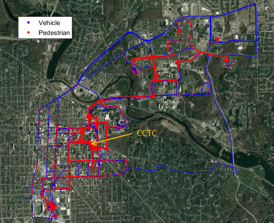
Figure 2: Routes of the instrumented buses and detected pedestrians in Ann Arbor, Michigan. The Central Campus Transit Center (CCTC) has a high pedestrian density. The figure is created based on Google Maps.

The unsignalized crossing chosen for collecting data is in Ann Arbor, Michigan, near the University of Michigan’s Central Campus Transit Center (CCTC), where the pedestrian density is high (Fig. 2). The geographic location is $42.278415^{\circ}$, $-83.735580^{\circ}$. A picture of this crossing path is shown in Fig. 3, where 2,973 valid passing events were collected.

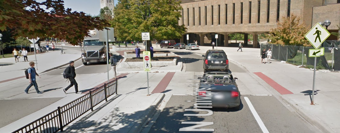
Figure 3: Crossing path environment (based on Google Maps)

The GPS system recorded the latitude and longitude of the instrument vehicles, while the MobilEye^® recorded the relative positions of pedestrians. Using the data collected, each passing event was drawn in a Cartesian Coordinate system, so that the trajectories of the vehicles and pedestrians could be observed. One example is shown in Fig. 4. The color bar indicates the time of the samples.

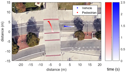
Figure 4: Sample of passing events (based on Google Maps)

III Interaction Model

A multivariate Gaussian mixture model is created based on naturalistic data to simulate the movement of vehicles and pedestrians when encountering unsignalized crossings. This stochastic model demonstrates how vehicles and pedestrians will interact with each other. This section shows the procedures used to develop this model and how to use it for the simulation.

III-A Variables

Appropriate variables must first be selected to develop a multivariate Gaussian mixture model. We simplified the passing scenario by assuming that the trajectories of the vehicle and the pedestrian are two perpendicular straight lines. Then, longitudinal distance ($R$) and lateral distance ($L$) are used to describe the relative position of a pedestrian (Fig. 5).

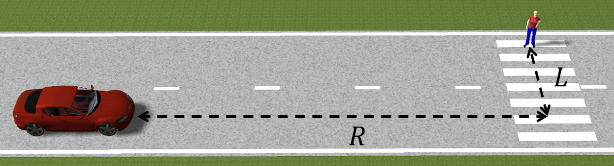
Figure 5: Definition of $R$ (longitudinal distance) and $L$ (lateral distance)

Four variables are required to define the state of the passing scenario: the reciprocal of the longitudinal distance ($R^{-1}$), vehicle speed ($v$), pedestrian walking speed ($v_{p}$) and the reciprocal of the Time Advantage ($T_{Adv}^{-1}$). Time Advantage is an indicator used to describe situations where two road users pass a common spatial zone, but at different times, thus avoiding a collision [17]. The definition of Time Advantage is the time between the first road user leaving the common spatial zone and the second arriving. The mathematical definition is:

$$T_{Adv}=|TTC-L/v_{p}|.$$ (1)

The reciprocals are used for statistical convenience. Among the four variables, $R^{-1}$ and $v$ can be obtained by the instrumented vehicle directly, $T_{Adv}^{-1}$ can be calculated by (1), and $v_{p}$ can be calculated by the lateral distance ($L$) data.

III-B Algorithms

The probability density function ($p.d.f.$) of a Gaussian mixture model is

$$f(y;\Theta)=\sum_{k=1}^{K}\pi_{k}f_{k}(y;\theta_{k}),$$ (2)

where $\pi_{k}$ are weights of components, $f_{k}$ are density functions of each component, $\theta_{k}$ are parameters to decide each component. The distribution of each component is a multivariate Gaussian distribution with mean $\mu_{k}$ and covariance $\Sigma_{k}$.

Algorithms are required to fit Gaussian mixture models to the traffic data. Here, since all the variables (i.e., $R^{-1}$, $v$, $v_{p}$, $T_{Adv}^{-1}$) are positive and have boundaries, a truncated Gaussian mixture model will better fit the data. Lee et al. [18] developed for fitting multivariate Gaussian mixture models to data that is truncated. By applying these algorithms to the data, parameters $\pi_{k}$, $\mu_{k}$ and $\Sigma_{k}$ of the multivariate Gaussian mixture model can be calculated.

The number of components ($K$) of the multivariate Gaussian mixture model will influence how well the data fit, with a higher $K$ helping to improve the precision of the modeling. However, it might also lead to greater computing time, as well as statistical errors such as singular covariance matrices which endanger the stability of the model. Thus, an appropriate $K$ must be selected for the Gaussian mixture model. The Bayesian information criterion (BIC) provides a means for model selection. It can help estimate the quality of the statistical models, with a model with a lower BIC preferred. In the interaction model, this criterion was used to determine the appropriate value of $K$, the BIC of the Gaussian mixture models with different $K$ can be seen in Fig. 6. The BIC continues to decrease with an increase in number of components, with little change in rate (less than 10%) when the number of components is larger than 10. Considering the computing time and the complexity of the models, $K$ = 10 was selected when generating the multivariate Gaussian mixture model.

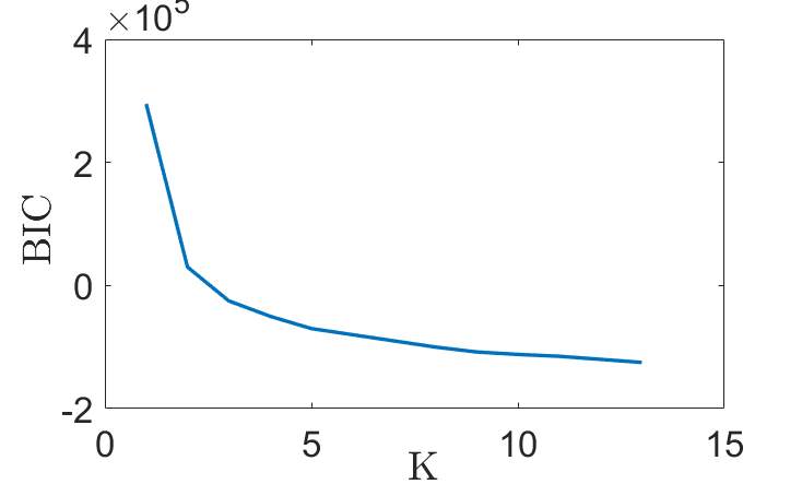
(a) Change of BIC

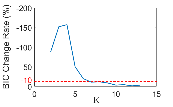
(b) Change Rate of BIC

Figure 6: Bayesian Information Criterion test of the interaction models with different number of components ($K$). The BIC continues to decrease with an increase in number of components, with little change in rate (less than 10%) when the number of components is larger than 10.

An interaction model was then created by fitting a 10-component truncated multivariate Gaussian mixture model to the collected naturalistic data using the algorithms above.

III-C Model Display and Utilization

Since there were four variables (i.e., {$R^{-1}$, $v$, $v_{p}$, $T_{Adv}^{-1}$}) in the Gaussian mixture model, the distribution of the interaction model was a 4-D function, which cannot be shown effectively on a flat piece of paper. We projected the function to three 2-D functions to illustrate the probability distribution, and then compared them with the raw data collected. The results are shown in Fig. 7.

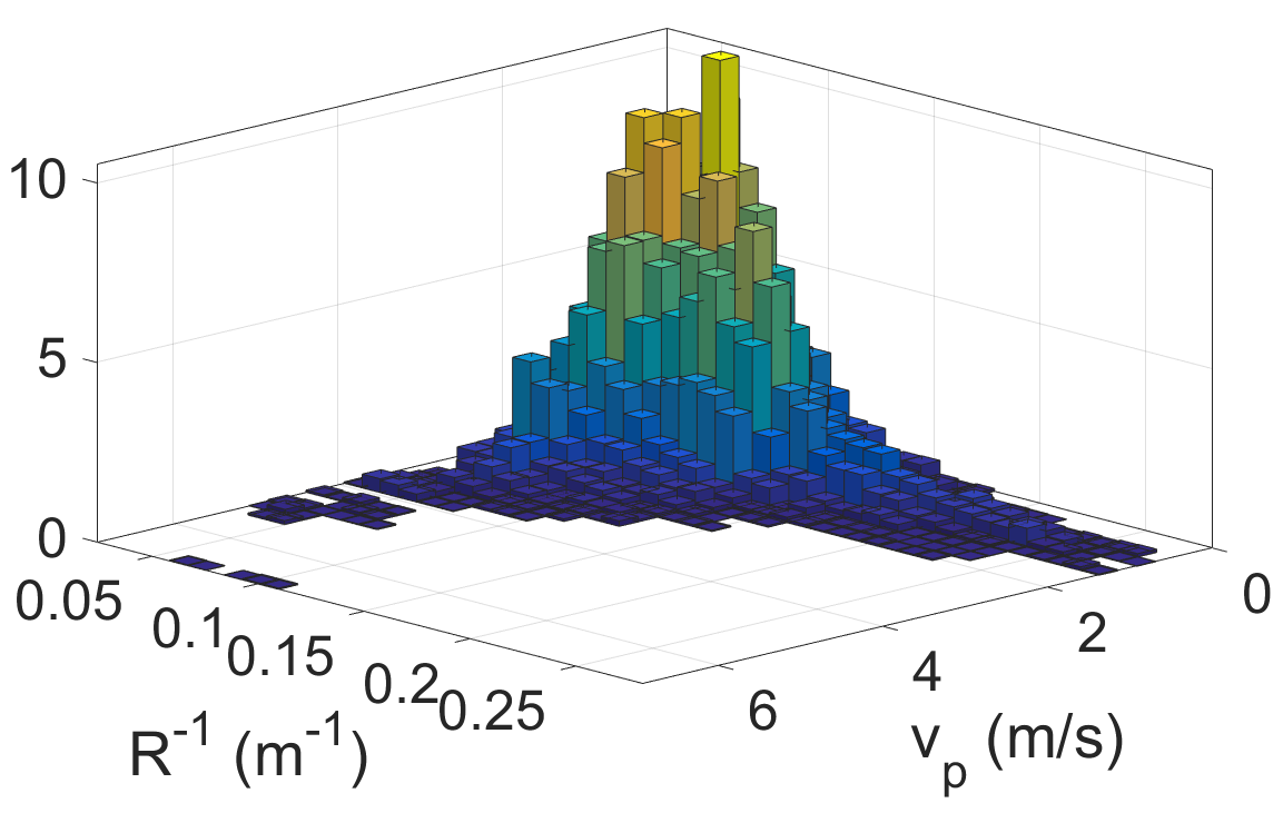
(a) Raw data

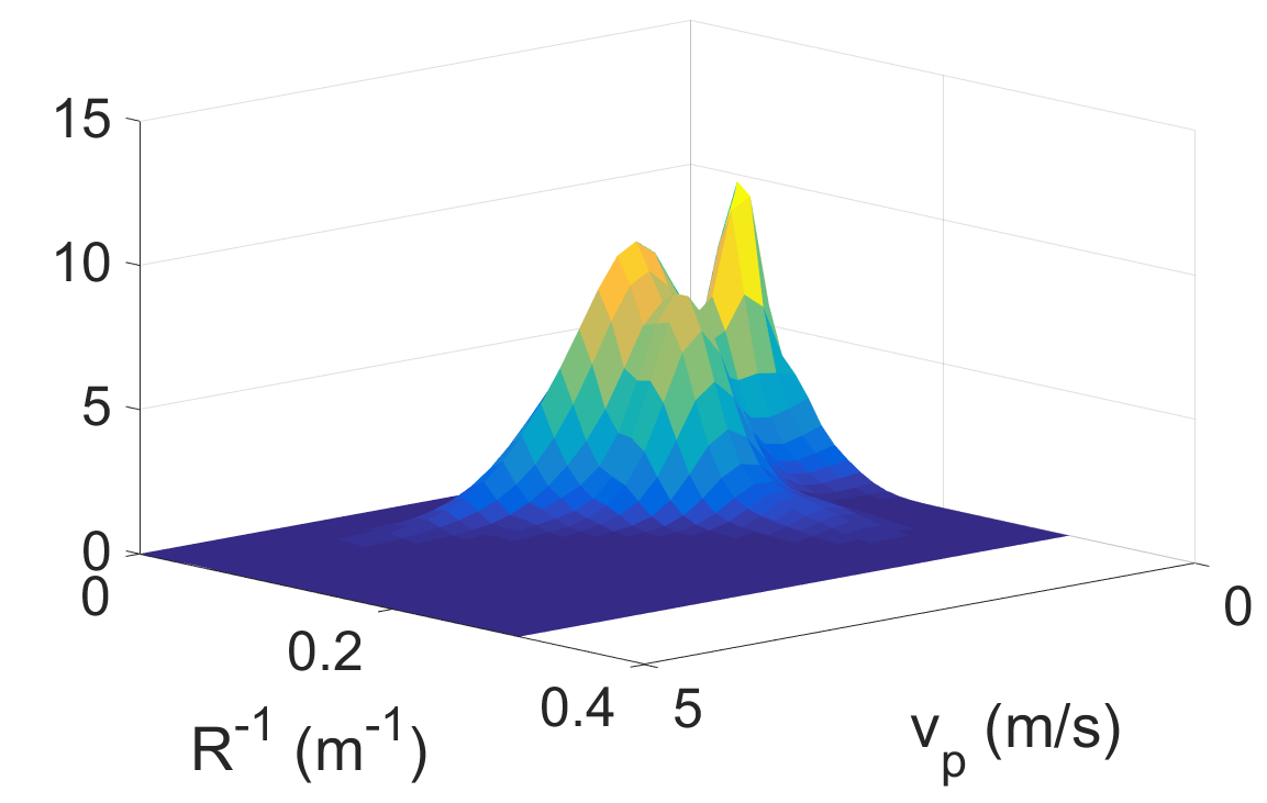
(b) Model distribution

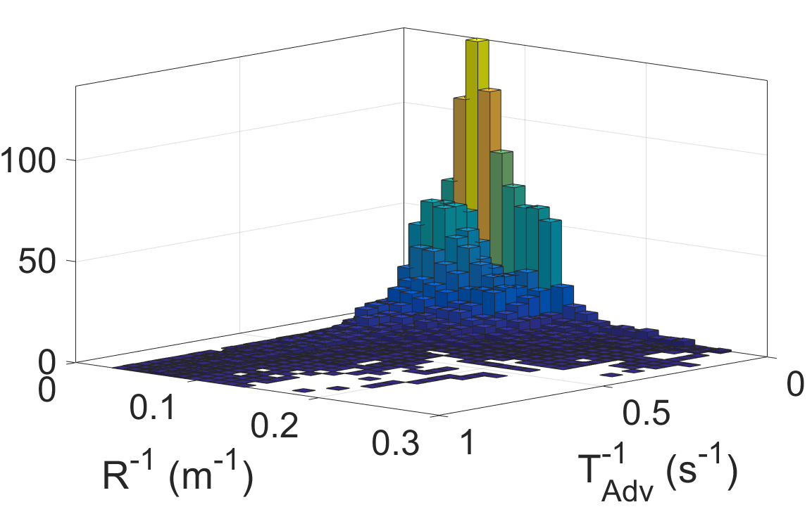
(c) Raw data

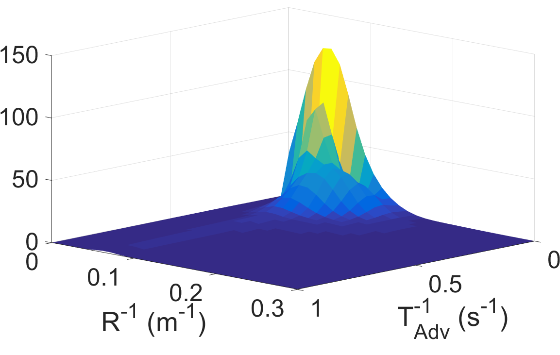
(d) Model distribution

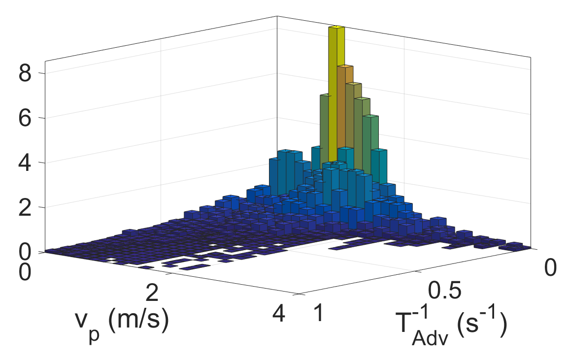
(e) Raw data

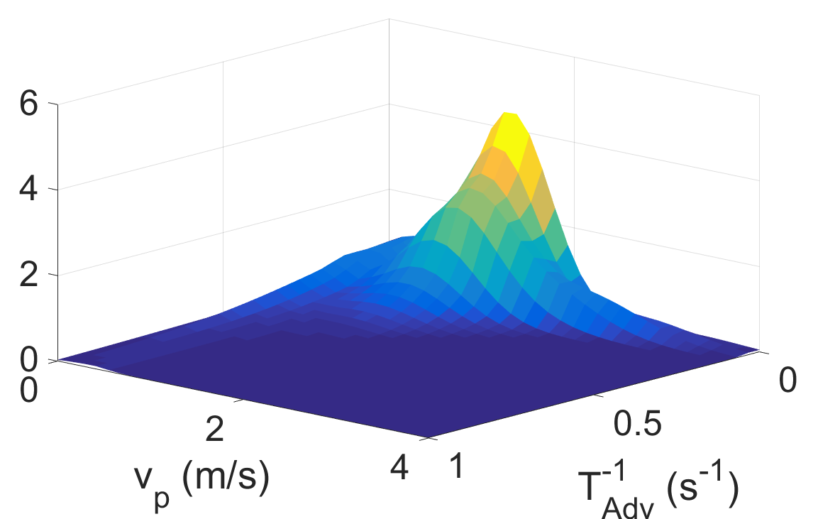
(f) Model distribution

Figure 7: Comparison of raw data and Gaussian mixture model

The stochastic interaction model developed here can help to simulate the walking speed of pedestrians. When encountering an unsignalized crossing, the pedestrian will decide the appropriate walking speed to cross the street, depending on the speed and position of the oncoming vehicle; that is, the distribution of pedestrian walking speed ($v_{p}$) is a conditional distribution of the multivariate Gaussian mixture model. By calculating this conditional distribution, the walking speed of pedestrians ($v_{p}$) can be simulated.

For a Gaussian distribution, if $y=(y^{T}_{m},y^{T}_{o})^{T}$ is with mean $\mu$ and covariance $\Sigma$, then the conditional distribution of $y_{m}|y_{o}$ is also normally distributed with mean and covariance:

$$\mu_{m|o}=\mu_{m}+\Sigma_{m,o}\Sigma_{o,o}^{-1}(y_{o}-\mu_{o}),$$ (3)

$$\Sigma_{m|o}=\Sigma_{m,m}-\Sigma_{m,o}\Sigma_{o,o}^{-1}\Sigma_{o,m}.$$ (4)

To calculate the conditional distribution of a mixture Gaussian model, first calculate the conditional distribution of each component, then normalize all components and set new weights.

If we set $y_{m}=v_{p}$ and $y_{o}=\{R^{-1},v,T_{Adv}^{-1}\}$, then the distribution function of $v_{p}$ under given conditions can be calculated. Examples of distribution functions under different conditions are shown in Fig. 8. We can generate a random $v_{p}$ from this distribution and take it as the walking speed of a pedestrian under the given conditions for the simulation and evaluation.

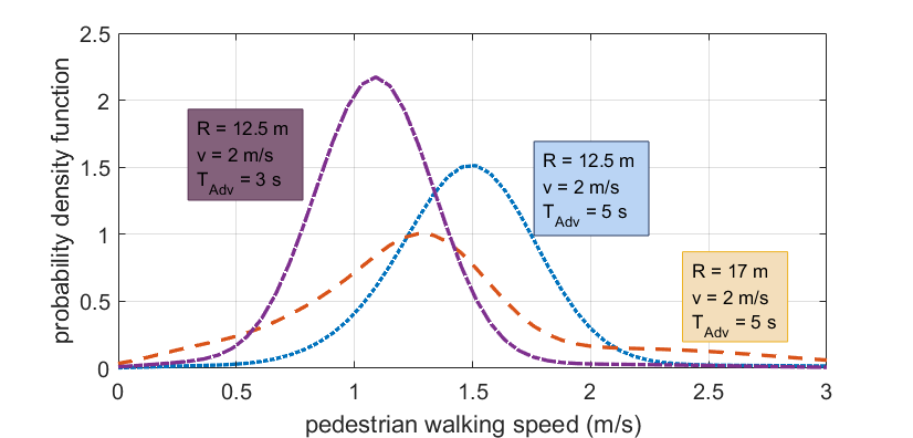
Figure 8: Probability density functions of pedestrian walking speed under different conditions

The movement of vehicles can also be simulated using the same method by calculating the conditional distribution. To do that, we set $y_{m}=v$ and $y_{o}=\{R^{-1},v_{p},T_{Adv}^{-1}\}$, and then the distribution function of $v$ can be calculated. Examples of distribution functions under different conditions are shown in Fig. 9. It is clear that, in this model, the vehicle is likely to have a lower speed when the distance is shorter, which makes sense considering traffic safety. The speed with the highest probability might be a good choice for setting the desired speed of the vehicle under given conditions when designing driving strategy.

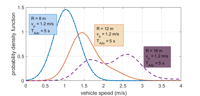
Figure 9: Probability density functions of vehicle speed under different conditions

IV Simulation

A simulation is used to show how to evaluate the driving strategy of automated vehicles. The automated vehicle is evaluated against the human drivers for better performance when encountering unsignalized crossings in the simulation. We expect that the driving strategy of automated vehicles be neither too aggressive (endangering traffic safety) nor too conservative (leading to traffic congestion). With an increase in aggressiveness of the automated vehicle, less time is then needed to pass through the intersection, resulting in a possible rise in the crash rate. As shown in Fig. 10, the aggressiveness needs to be within the allowed interval when the automated vehicle has a passing time less of than $\mu_{0}$ and a denied crash rate less than $\kappa_{0}$.

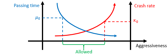
Figure 10: Influence of the vehicle’s aggressiveness

IV-A Procedures for the Evaluation Experiment

PreScan^® is used for the simulation. The experiment takes place at an unsignalized crossing (Fig. 11). At first, the vehicle comes from a long distance at a constant speed $v_{0}$. When it is close, at a certain distance $R_{0}$, pedestrians will start to be generated to go across the street, and the vehicle will interact with pedestrians and try to pass through the intersection without any crashes. Each experiment is done twice. The first time, the automated vehicle is tested to interact with the pedestrians; the second time, the human driver passing strategy is applied to interact with the same pedestrian which is recorded as a reference for the evaluation. In this study, the simulation is run 50 times. The passing strategies of pedestrians, automated vehicles and human drivers simulated in this section are described below separately. The results are analyzed at the end of this section.

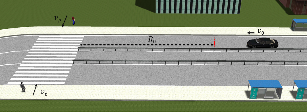
Figure 11: Environment of the simulation. When the vehicle is at a certain distance ($R=R_{0}$), pedestrians will start to arrive at the unsignalized crossing.

IV-B Pedestrian Crossing Strategy

Pedestrians are made to cross the street from both sides. When the vehicle is at a certain distance ($R=R_{0}$), pedestrians will start to arrive at the unsignalized crossing. Each pedestrian has an arriving time when they will be put on the side of the street and start to cross. The arriving time of the pedestrians obeys the Poisson process:

$$P\{N(t)=n\}=\frac{(\lambda t)^{n}}{n!}e^{(-\lambda t)}.$$ (5)

Parameter $\lambda$ can be set to different values depending on the density of pedestrian flow, which varies greatly depending on time and location. For reference, pedestrian flow in the campus area during peak hours is around 250 peds/hr [13]. Based on this distribution, an arriving time example was generated and is shown in Fig. 12. Five pedestrians are scheduled to arrive at this crossing within 60 seconds.

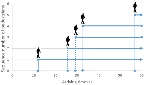
Figure 12: Arriving times of pedestrians within 60 seconds

Though the pedestrians’ arriving times are random, their walking speeds are usually not. Each pedestrian has a constant walking speed that is calculated by the interaction model depending on the distance and speed of the oncoming vehicle when the pedestrian arrives, which is similar to real world process, in which most pedestrians will look at the oncoming vehicle and decide what to do before moving.

IV-C Automated Vehicle’s Passing Strategy

The driving strategy evaluated in the simulation is the Soft-Yield model proposed by Schroeder et al. [13] which provides vehicle trajectories when facing one pedestrian.

The model was developed based on GPS data from the instrumented vehicle study. The generalized vehicle distance-speed and time-speed models are shown in Fig. 13. When approaching the unsignalized crossing, the vehicle has a constant deceleration for time length $T_{1}$ and then starts to coast to the crosswalk.

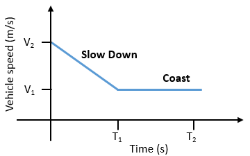
Figure 13: Driving strategy of the automated vehicle when encountering an unsignalized crossing (developed by Schroeder et al. [13])

Based on a regression analysis, vehicle acceleration $a$ is set to

$$a=p_{1}+p_{2}v+p_{3}R,$$ (6)

where $p_{1}=0.0169$, $p_{2}=-0.13986$, $p_{3}=0.010115$. $v$ and $R$ are the vehicle’s information when the vehicle perceives the pedestrian and makes its decision.

Deceleration time $T_{1}$ is calculated as follows:

$$t_{L}=\frac{L_{0}}{v_{p}},$$ (7)

$$T_{1}=t_{L}-\sqrt{t_{L}^{2}-\frac{2(R-v*t_{L})}{a}},$$ (8)

where $L_{0}$ is the length of the crossing path, and $t_{L}$ is the time needed for the pedestrian to complete the crossing.

IV-D Human Driver’s Passing Strategy

A human driver’s passing strategy was developed by studying the interaction model based on the naturalistic traffic data. When encountering an unsignalized crossing, the strategy of the simulated human driver is set to adjust the vehicle’s speed if a pedestrian is detected. The desired speed $v_{d}$ for adjusting is calculated based on the position and velocity of the pedestrian in the current state. Thus, the desired acceleration of the vehicle is

$$a_{d}=\frac{v_{d}-v}{\Delta t},$$ (9)

where $\Delta t$ is the time interval between two updates of the desired speed. In this study, we set $\Delta t$ = 1 s.

Each vehicle, of course, has a maximum limit of acceleration $a_{m}$. Thus, if $a_{d}>a_{m}$, the acceleration of the vehicle $a$ will be set to $a=a_{m}$. Otherwise, the acceleration will be set to just $a=a_{d}$.

When no pedestrian is present within the radar’s detection range, or the pedestrians have left the crossing, the vehicle will accelerate to $v_{0}$ at a constant speed of $a_{0}$ = 1 m/s.

IV-E Simulation Results

All the above procedures are simulated using PreScan^®. The parameters set for the simulation is shown in Table I. One pedestrian is generated in each experiment.

TABLE I: Parameters in the simulation

symbol	unit	value
$R_{0}$	m	30
$L_{0}$	m	9
$v_{0}$	m/s	5

Each experiment is done twice. The first time, the automated vehicle’s strategy is tested to interact with the pedestrians generated based on the Poisson process; the second time, the human driver’s strategy is tested to interact with the same pedestrian. The time used and the safety of the pedestrian is recorded. We evaluate the aggressiveness of the automated vehicle by analyzing its results compared to those of the human driver strategy.

Assume $t_{a}^{i}$ and $t_{h}^{i}$ are the time used by the automated vehicle and the human driver for passing through the unsignalized crossing in experiment $i$, respectively. Then, $\tau_{i}=t_{a}^{i}/t_{h}^{i}$ indicates the efficiency of the automated vehicle compared to the human driver. After $N$ = 50 experiments, the mean value and distribution of $\{\tau_{i}\}$ is shown in Fig. 14. As $n$ increases, the mean value of $\{\tau_{i}\}$ approaches a limit value, which means that the time used by the automated vehicle to pass through the intersection is stable.

Figure 14: Mean value and distribution of $\{\tau_{i}\}$ (the ratio of time used in experiments $i$). As the number of simulated experiment increases, the mean value of $\{\tau_{i}\}$ approaches a limit value.

$\mu$ (The mean value of $\{\tau_{i}\}$), $c_{v}$ (the coefficient of variation of $\{\tau_{i}\}$) and $\kappa$ (the crash rate) are parameters to indicate the passing strategy’s efficiency, stability and safety, respectively. They are calculated to evaluate the automated vehicle based on the experimental results:

$$\mu=\frac{\sum\tau_{i}}{N}=0.7044,$$ (10)

$$c_{v}=\frac{\sigma}{\mu}=\frac{\sqrt[]{\frac{1}{N}\sum_{i=1}^{N}(\tau_{i}-\mu)^{2}}}{\mu}=4.54\%，$$ (11)

$$\kappa=\frac{n_{crash}}{N}=0.$$ (12)

It turns out that the passing strategy of the automated vehicle is more efficient than that of a human driver, taking only about 70% of the time a human driver uses to pass the unsignalized crossing. It is also quite stable since $c_{v}$ is under 5%. More importantly, no crash occurred during the simulation, meaning the strategy is also safe under ideal conditions.

V Conclusion and Discussion

In this paper, we proposes a method to evaluate the passing strategy of automated vehicles at unsignalized crossings. A stochastic interaction model is developed to predict pedestrian movement. A simulation is conducted to demonstrate the evaluation procedure. The automated vehicle is evaluated against the human drivers for better performance in terms of the time used and the crash rate. One Soft-Yield driver model is evaluated as an example. The simulation results indicate that this driving strategy is more efficient than that of a human driver that is modeled by naturalistic data collected in Ann Arbor.

The pedestrians in our evaluation experiments comes from both sides of the crossing. Their arriving times obey the Poisson process; the density of pedestrian flow can be adjusted by setting different values of parameters. The pedestrians in the simulation will have a look at the oncoming vehicle and then decide on their walking speed before moving, similar to the process in the real world. However, a more detailed pedestrian model remains to be developed, and more behaviors and features can be taken into account in future work.

Disclaimers

This work was funded in part by the University of Michigan Mobility Transformation Center Denso Tailor project. The findings and conclusions in the report are those of the authors and do not necessarily represent the views of the MTC or Denso.

References

- [1] N. Highway Traffic Safety Administration and U. Department of Transportation, “Research Note 2015 Motor Vehicle Crashes Overview,” no. August, 2016.
- [2] D. Zhao, H. Lam, H. Peng, S. Bao, D. J. Leblanc, and C. S. Pan, “Accelerated Evaluation of Automated Vehicles Safety in Lane Change Scenarios based on Importance Sampling Techniques,” IEEE Transactions on Intelligent Transportation Systems, 2016.
- [3] D. Zhao, X. Huang, H. Peng, H. Lam, and D. J. LeBlanc, “Accelerated Evaluation of Automated Vehicles in Car-Following Maneuvers,” submitted to IEEE Transactions on Intelligent Transportation Systems, 7 2017. [Online]. Available: http://arxiv.org/abs/1607.02687
- [4] Z. Huang, D. Zhao, H. Lam, and D. J. LeBlanc, “Accelerated Evaluation of Automated Vehicles Using Piecewise Mixture Models,” submitted to IEEE Transactions on Intelligent Transportation Systems, 7 2017. [Online]. Available: http://arxiv.org/abs/1701.08915
- [5] C. Burstedde, K. Klauck, A. Schadschneider, and J. Zittartz, “Simulation of pedestrian dynamics using a two-dimensional cellular automaton,” Physica A Statistical Mechanics and its Applications, vol. 295, no. 3-4, pp. 507–525, 2001.
- [6] M. Chraibi, A. Seyfried, A. Schadschneider, and W. MacKens, “Quantitative description of pedestrian dynamics with a force-based model,” Proceedings-2009 IEEEWICACM International Conference on Web Intelligence and Intelligent Agent Technology-Workshops, WI-IAT Workshops 2009, vol. 3, pp. 583–586, 2009.
- [7] T. Xiong, P. Zhang, S. C. Wong, C.-W. Shu, and M.-P. Zhang, “A Macroscopic Approach to the Lane Formation Phenomenon in Pedestrian Counterflow,” Chinese Physics Letters, vol. 28, p. 108901, 2011.
- [8] S. Bennett, A. Felton, and R. Akccelik, “Pedestrian movement characteristics at signalised intersections,” 23rd Conference of Australian Institutes of Transport Research, no. December, pp. 10–12, 2001.
- [9] M. S. Tarawneh, “Evaluation of pedestrian speed in Jordan with investigation of some contributing factors,” Journal of Safety Research, vol. 32, no. 2, pp. 229–236, 2001.
- [10] D. Yagil, “Beliefs, motives and situational factors related to pedestrians? self-reported behavior at signal-controlled crossings,” Transportation Research Part F Traffic Psychology and Behaviour, vol. 3, pp. 1–13, 2000.
- [11] B. Dazhi Sun, S. VSK Ukkusuri, R. F. Benekohal, S. Travis Waller, D. Sun, R. F. Benekohal, and S. T. Waller, “Modeling of Motorist-Pedestrian Interaction at Uncontrolled Mid-block Crosswalks,” no. November, 2002.
- [12] B. B. J. Schroeder, “A Behavior-Based Methodology for Evaluating Pedestrian-Vehicle Interaction at Crosswalks,” Analysis, p. 332, 2008.
- [13] B. Schroeder, N. Rouphail, K. Salamati, E. Hunter, B. Phillips, L. Elefteriadou, T. Chase, Y. Zheng, V. Sisiopiku P, and S. Mamidipalli, “Empirically-Based Performance Assessment and Simulation of Pedestrian Behavior at Unsignalized Crossings,” no. September, 2014.
- [14] Keisuke Suzuki, Takuya Kakihara, and Yasutoshi Horii, “Investigation of Braking Timing of Drivers for Design of Pedestrian Collision Avoidance System,” Journal of Mechanics Engineering and Automation, vol. 6, no. 3, pp. 118–127, 2016.
- [15] Euro-NCAP, “Euro NCAP Test Protocol - AEB VRU systems,” no. 1.0.1, 2015. [Online]. Available: httpwww.euroncap.comenfor-engineersprotocolssafety-assist
- [16] D. Bezzina and J. Sayer, “Safety pilot model deployment: Test conductor team report,” Report No. DOT HS, vol. 812, p. 171, 2014.
- [17] A. Laureshyn, s. Svensson, and C. Hyd’en, “Evaluation of traffic safety, based on micro-level behavioural data Theoretical framework and first implementation,” Accident Analysis and Prevention, vol. 42, no. 6, pp. 1637–1646, 2010.
- [18] G. Lee and C. Scott, “EM algorithms for multivariate Gaussian mixture models with truncated and censored data,” Computational Statistics and Data Analysis, vol. 56, no. 9, pp. 2816–2829, 2012.