Convergence of Stochastic Approximation Monte Carlo and
modified Wang-Landau algorithms: Tests for the Ising model

Abstract

We investigate the behavior of the deviation of the estimator for the density of states (DOS) with respect to the exact solution in the course of Wang-Landau and Stochastic Approximation Monte Carlo (SAMC) simulations of the two-dimensional Ising model. We find that the deviation saturates in the Wang-Landau case. This can be cured by adjusting the refinement scheme. To this end, the $1/t$-modification of the Wang-Landau algorithm has been suggested. A similar choice of refinement scheme is employed in the SAMC algorithm. The convergence behavior of all three algorithms is examined. It turns out that the convergence of the SAMC algorithm is very sensitive to the onset of the refinement. Finally, the internal energy and specific heat of the Ising model are calculated from the SAMC DOS and compared to exact values.

1 Introduction

The Wang-Landau algorithm [1, 2] has proven to be a very efficient tool for determining the density of states (DOS) of statistical systems near phase transitions where traditional local importance sampling algorithms like the Metropolis algorithm are likely to run into critical slowing down or become trapped in local free-energy minima [3]. It has, however, been pointed out that the error of the estimator for the DOS obtained by the Wang-Landau algorithm cannot be made arbitrarily small just by using longer simulations [4], the (systematic) error saturates at some (small) value. To overcome this, it has been suggested to change the behavior of the refinement parameter in the $1/t$ modification ($1/t$-WL) of the Wang-Landau algorithm in order to circumvent the error saturation [5, 6, 7].

Another approach is the Stochastic Approximation Monte Carlo (SAMC) algorithm first introduced in Ref. [8] and refined in Ref. [9], which works similar to the modified Wang-Landau algorithm regarding the choice of refinement scheme. While the algorithm proposed by Belardinelli and Pereyra has been tested for the Ising model [5, 6], for the calculation of multidimensional integrals [10] and was applied to lattice polymer models [11], the SAMC algorithm has only been tested for an artificial, non-physical model with a very small number of states [9] compared to models currently studied in statistical physics and for an off-lattice polymer model [12].

The standard test case, the Ising model, however, is still missing. After summarizing a few basic properties of this paradigm model needed for our purposes in the next section, we discuss briefly the behavior of the Wang-Landau and $1/t$-WL algorithms in Sections 3 and 4, confirming the results of Belardinelli and Pereyra. In Section 5 we describe the SAMC algorithm and in Section 6 we present our results on the accuracy of the SAMC algorithm applied to the two-dimensional Ising model for long simulation times. Finally, Section 7 contains our conclusions.

2 The Ising model

First introduced in 1D by Ernst Ising in 1925 in his doctoral thesis [13], the generalisation of the Ising model to higher dimensions, especially 2D and 3D, has become the “drosophila of computational physics”. Despite its conceptual simplicity it shows nontrivial behavior already in the 2D case like a temperature-driven continuous phase transition at finite temperature. The model consists of a lattice of spins $s_{i}$ which can take the values $s_{i}=\pm 1$. The Ising Hamiltonian reads

$$H=-J\sum\limits_{\langle i,j\rangle}s_{i}s_{j}-h\sum\limits_{i}s_{i}\;,$$ (1)

where $\langle i,j\rangle$ denotes a sum only over nearest-neighbour spins, the coupling constant $J$ sets the energy scale and $h$ is an external magnetic field. The partition function of the 2D Ising model with periodic boundary conditions was found by Lars Onsager in the infinite-volume limit for the case $h=0$ in 1944 [14] and extended to finite square lattices by Kaufman in 1949 [15]. An easy way to compute the DOS for finite lattices was only found much later by Beale [16] using the fact that it is possible to rewrite the partition function $Z$ in the following way:

$$Z=\sum_{\mu}e^{-\beta H}=\sum_{E}g(E)e^{-\beta E}\;,$$ (2)

where $\beta=1/k_{\mathrm{B}}T$ and $g(E)$ denotes the number of microstates with energy $E$. The first sum is over all possible microstates $\mu$ while the second is carried out over all energies available to the system. The quantity $g(E)$ is identical to the density of states. The results of Beale will be used in the following to compare the performances of the SAMC and Wang-Landau algorithms.

3 Error saturation in the Wang-Landau algorithm

Figure 1: (left) The behavior of the average deviation from the exact solution $\langle\epsilon(t)\rangle_{E}$ for the $8\times 8$ Ising model for the Wang-Landau and $1/t$-WL algorithm over attempted spin flips (MC time) $t$ for different flatness parameters $m$. The data was obtained by averaging over 40 independent runs of the algorithm to reduce statistical noise. (right) The behavior of the average deviation from the exact solution $\langle\epsilon(t)\rangle_{E}$ and the logarithm $F$ of the refinement parameter over MC time $t$ for one single simulation with flatness parameter $m=0.8$ with extended $y$-range to show the behavior of $F$.

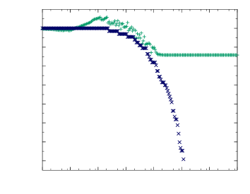
The Wang-Landau algorithm attempts to sample the density of states $g(E)$ by ensuring that during the simulation each energy is visited equally often. This is equivalent to sampling with probability proportional to $g^{-1}(E)$ . Because the DOS is a-priori unknown, this is done by starting with a very rough estimator $\widehat{g}(E)$ for $g(E)$, usually $\widehat{g}(E)=1$ for all values of $E$. One also needs to keep track of the histogram $H(E)$, which stores the number of times the states with energy $E$ are visited during the simulation. The density of states $\widehat{g}(E)$ is then refined using a parameter $f$, usually set to $f=e=2.71828...$ initially. The refining process works as follows:

1. Pick a starting state $\mu$ and calculate its energy $E_{\mu}$. Set $H(E)=0$ and $\widehat{g}(E)=1$ for all energies

2. Propose a randomly chosen update to get a new state $\nu$ with energy $E_{\nu}$

3. Calculate $\widehat{g}(E_{\mu})/\widehat{g}(E_{\nu})$

   1. if $\widehat{g}(E_{\mu})/\widehat{g}(E_{\nu})\geq 1$ accept the update and set
      $\widehat{g}(E_{\nu})\rightarrow\widehat{g}(E_{\nu})\cdot f$ and
      $H(E_{\nu})\rightarrow H(E_{\nu})+1$

   2. if $\widehat{g}(E_{\mu})/\widehat{g}(E_{\nu})<1$ accept the update with probability $\widehat{g}(E_{\mu})/\widehat{g}(E_{\nu})$

      1. If accepted, set
         $\widehat{g}(E_{\nu})\rightarrow\widehat{g}(E_{\nu})\cdot f$ and
         $H(E_{\nu})\rightarrow H(E_{\nu})+1$

      2. If rejected, set
         $\widehat{g}(E_{\mu})\rightarrow\widehat{g}(E_{\mu})\cdot f$ and
         $H(E_{\mu})\rightarrow H(E_{\mu})+1$

4. After a suitable number (e.g. 1000) of repetitions of steps (2-3), check the histogram for flatness.

   1. If the histogram is not flat, go back to step 2

   2. If the histogram is flat, reset $H(E)$ to $0$ for all values of $E$, adjust $f\rightarrow f^{\frac{1}{2}}$, then go to step 5

5. Check whether $f$ is smaller than some predefined final value $f_{\text{final}}$.

   1. If $f$ is not smaller than $f_{\text{final}}$, go back to step 2

   2. If $f$ is smaller than $f_{\text{final}}$, the calculation is finished and $\widehat{g}(E)$ obtained during the simulation is an estimator for the real density of states

We use a slight variation of the algorithm: Since our goal is to reproduce the error saturation, we do not terminate the algorithm at a certain value $f_{\text{final}}$, but run it as long until we observe the saturation of the error. It is convenient to work with the logarithms of the values $S:=\ln\widehat{g}$ and $F:=\ln f$ in order to fit the large numbers into double precision variables and to replace the multiplication $\widehat{g}\cdot f$ by an addition $S+F$. Physically, $S(E)$ is the (configurational) microcanonical entropy (in units where $k_{\mathrm{B}}=1$) [17]. One sees that for long simulation times, the flatness criterion is satisfied in every iteration of the algorithm, provided that the time between subsequent flatness checks is long enough. Thus the refinement parameter $F$ is made smaller in every iteration, which means that it decreases geometrically. This has been shown to prevent the convergence of the error to zero [5]. A somewhat subtle point in the Wang-Landau algorithm is the notion of flatness. Here we use the criterion that the histogram is flat, if for all energies $E$, $H(E)$ falls into the interval $\left[m\overline{H},(2-m)\overline{H}\right]$, where $\overline{H}$ denotes the average value of the histogram and $m$ is the so called flatness parameter, usually chosen between $0.7$ and $1$. The flatness parameter, however, cannot overcome the fundamental saturation problem of the Wang-Landau algorithm, the saturation just sets in at a lower deviation value for higher $m$ [5]. On the left of Fig. 1 the behavior of the average deviation from the exact solution,

$$\langle\epsilon(t)\rangle_{E}=\frac{1}{N_{E}-1}\sum_{E}\left|\frac{S(E,t)-S_{\text{Beale}}(E)}{S_{\text{Beale}}(E)}\right|\;,$$ (3)

during Wang-Landau simulations of the $8\times 8$ Ising model is shown. Here, we have introduced the Monte Carlo (MC) time $t$ in units of updates in the sense of step 2 of the Wang-Landau algorithm, $N_{E}$ denotes the number of different energy values and $S_{\text{Beale}}$ is the exact value of $S$ from the Beale solution [16]. In case of the Ising model, the update is the spin flip of a uniformly randomly chosen spin. The estimator $S(E,t)$ is normalized with respect to the exact DOS of the ground states. It is visible that the deviation saturates, even for the strictest choice of flatness parameter, reproducing the results of Belardinelli and Pereyra [5]. On the right of Fig. 1 the behavior of the logarithm $F$ of the refinement parameter $f$ during the saturation phase is depicted. From the beginning of the saturation phase, it decreases too fast to correct the estimator for the DOS significantly.

4 The 1/t-modification of the Wang-Landau algorithm

The error saturation can be corrected by appropriately adapting the refinement parameter in order to prevent its fast decrease. This was suggested by Belardinelli and Pereyra in Ref. [6]. Their algorithm avoids the notion of flatness of the histogram and, in the first phase, only checks whether all energies have been visited and refined at least once by the current $F_{t}$. If $F_{t}\leq N_{E}/t$, where $N_{E}$ denotes the number of energies available to the system, the algorithm enters its second phase, the histogram is no longer checked and $F_{t}$ is updated each simulation step $t$ according to $F_{t}=N_{E}/t$. For long times, $F_{t}$ now converges much slower towards zero than in the original Wang-Landau case. This can avoid the saturation of the deviation as is shown in Fig. 1. The deviation for the $1/t$-algorithm does not saturate in the simulation time of $10^{9}$ attempted spin flips for the $8\times 8$ Ising model. Another limitation of the Wang-Landau algorithm, which is the fact that the energy range of the model needs to be known beforehand is still present in this algorithm: One needs to know all admissible energies of a system in order to discern between histogram bins that have not been visited by the algorithm yet, but are available to the system in principle, and histogram bins that can never be visited because the system can not access those energies. This is not a big problem in the Ising model, because the energy range is known here, but can be a problem for systems with unknown ground states like spin glasses or lattice polymers. An extension to the algorithm which can overcome this problem has been proposed in Refs. [18, 11].

Figure 2: (left) The behavior of the average deviation from the exact solution $\langle\epsilon(t)\rangle_{E}$ over MC time $t$ for the SAMC simulation of the $8\times 8$ Ising model (pluses) and of the square root $F^{1/2}$ of the refinement parameter $F$ (crosses). $t_{0}$ was chosen as $t_{0}=10^{5}$ here. The straight line is the graph of $t^{-1/2}$. This line is roughly parallel to the graph of the deviation. (right) The behavior of the average deviation from the exact solution for different choices of $t_{0}$. All data is averaged over 40 independent simulation runs in order to reduce statistical errors.

5 The SAMC algorithm

The SAMC algorithm [8, 9] is an algorithm which is based on stochastic approximation algorithms [19] and is similar to the Wang-Landau algorithm as it tries to obtain an estimator for the DOS by using a refinement parameter. The obtained estimator for the DOS is proven to converge to the real DOS almost surely if the sequence of refinement parameters $F_{t}$ satisfies

$$\sum_{t=1}^{\infty}F_{t}=\infty\quad\text{ and}\quad\sum_{t=1}^{\infty}F_{t}^{\zeta}<\infty\;.$$ (4)

for some $\zeta\in(1,2)$ along with necessary conditions on the proposal distribution [8, 9]. The Wang-Landau algorithm violates this criterion, as the sequence $F_{t}^{\text{WL}}$ is proportional to ${2^{-t}}$ for large $t$ and $\sum_{t=1}^{\infty}{2^{-t}}<\infty$ for Wang-Landau. The SAMC algorithm uses the sequence

$$F_{t}^{\text{SAMC}}=\frac{t_{0}}{\max(t_{0},t)}$$ (5)

instead, where $t_{0}>1$ is an arbitrary value which can be chosen according to the problem. This sequence fulfils both criteria because it behaves like $1/t$ for long simulation times and the harmonic series $\sum_{t=1}^{\infty}1/t$ diverges, while the series $\sum_{t=1}^{\infty}1/t^{\zeta}$ converges for $\zeta>1$. This is very similar to the $1/t$-WL case, where $F$ exhibits the same long-time behavior. Following Liang, Liu, and Carroll [9], one special case of their algorithm that aims for a flat histogram works as follows:

1. Pick a starting state $\mu$ and calculate its energy $E_{\mu}$. Set $S(E)=0$ for all energies

2. Randomly propose an update to get a new state $\nu$ with energy $E_{\nu}$

3. Calculate $e^{[S(E_{\mu})-S(E_{\nu})]}$

   1. if $e^{[S(E_{\mu})-S(E_{\nu})]}\geq 1$ accept the update and set $S(E_{\nu})\rightarrow S(E_{\nu})+F_{t}$

   2. if $e^{[S(E_{\mu})-S(E_{\nu})]}<1$ accept the update with a probability $e^{[S(E_{\mu})-S(E_{\nu})]}$

      1. If accepted, set $S(E_{\nu})\rightarrow S(E_{\nu})+F_{t}$

      2. If rejected, set $S(E_{\mu})\rightarrow S(E_{\mu})+F_{t}$

4. Go back to step 2, repeat the algorithm until $F_{t}$ is smaller than some predefined value.

One sees that the behavior of $F_{t}^{\text{SAMC}}$ is, in contrast to the Wang-Landau algorithm, fully deterministic, so the runtime of the algorithm can be predicted. Furthermore the SAMC algorithm avoids the checks for histogram flatness one has to do while using Wang-Landau by simply starting the decreasing behavior of $F_{t}$ at some defined time. The general algorithm provides the possibility to divide the energy space into subregions in order to perform a biased sampling [8, 9], which is not considered here, as the energy landscape of the Ising model is uncomplicated enough. Nevertheless, it has been noted before that sampling with other weight distributions than the inverse DOS can improve the quality of estimators obtained by Monte Carlo simulations [20]. An example of the impact of biased SAMC sampling is described in Ref. [12]. It should also be noted that none of the algorithms presented here can be viewed as a special case of Metropolis sampling with sampling distribution $g^{-1}(E)$ since the weights are perpetually modified. Therefore detailed balance is violated and the sampling process is non-Markovian.

6 Simulating the Ising model with SAMC

Figure 3: Green pluses: The behavior of the average deviation from the exact solution $\langle\epsilon(t)\rangle_{E}$ over MC time $t$ for the SAMC simulation of the $8\times 8$ Ising model. $t_{0}$ was chosen as $t_{0}=100$ here. Blue crosses: The behavior of $\Delta H/\overline{H}$ over MC time $t$. The data was obtained by averaging over 40 independent runs of the algorithm to reduce statistical noise.

Figure 4: (left) The behavior of the average deviation from the exact solution $\langle\epsilon(t)\rangle_{E}$ over MC time $t$ for SAMC for different $t_{0}$ and $1/t$-WL simulations of the $16\times 16$ Ising model. (right) The flatness of the histogram over MC time $t$ for different choices of $t_{0}$. The data was obtained by averaging over 40 independent runs of the algorithm to reduce statistical noise.

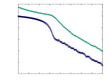
In this section we show the results of simulations of the Ising model for various lattice sizes using SAMC. The Hamiltonian for the Ising model without an external magnetic field is the special case $h=0$ of the Hamiltonian defined in Eq. (1). The deviation for the DOS with respect to the Beale solution is calculated according to Eq. (3) where $\widehat{g}(E)$ is normalized with respect to the exact DOS of the ground states. All simulations were started at one of the ground states of the Ising model, we chose all spins equal to $+1$. All data was obtained by averaging over 40 runs of the respective algorithms with independent seeds of the random number generator. Due to the symmetry of the density of states of the Ising model only the ferromagnetic states with energies from $E=E_{0}=-2L^{2}$ up to $E=0$ were considered.

6.1 The $8\times 8$ Ising model

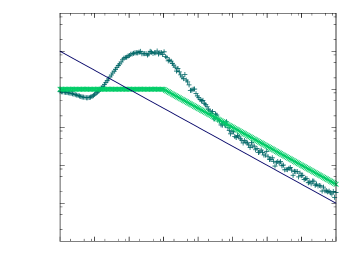
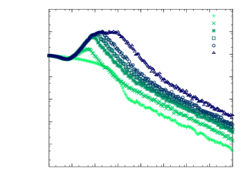
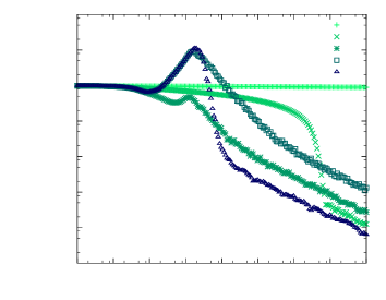
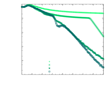
In Fig. 2 on the left side the behavior of the deviation from the exact solution and the refinement parameter during the run of the simulation for the $8\times 8$ Ising model with $t_{0}=10^{5}$ is shown. It is visible that, in the beginning, the deviation increases, which is due to the rough refinement with $F_{t}=1$. From the onset of the $F_{t}\propto 1/t$ behavior at $t=t_{0}=10^{5}$ however, the deviation steadily decreases until the end of the simulation which was even longer than the Wang-Landau simulations in Section 3. For later times, the deviation is proportional to $F^{1/2}\propto t^{-1/2}$, as indicated by the parallel lines in the double-logarithmic plot. This is similar to the findings of Belardinelli and Pereyra on their $1/t$-WL algorithm [6]. The attained deviation after $10^{9}$ updates is comparable to our least accurate estimator from the Wang-Landau simulation with $m=0.8$. This can be improved by choosing a more appropriate $t_{0}$. One sees that in the time between $10^{4}$ and $10^{5}$ updates the deviation stays at a constant, large value. In this phase the rough refinement with $F_{t}=1$ explores the energy landscape and reaches all available energies to ensure that the refinement can take place properly in the next stage. This does not necessarily generalize to more complicated models like lattice polymers, where some “hidden” (low) energies can only be visited when the estimator of the DOS is already sufficiently accurate [21]. In Fig. 2 on the right side, the behavior of the deviation for SAMC simulation of the $8\times 8$ Ising model is shown for various values of $t_{0}$ ranging from $t_{0}=100$ to $t_{0}=10^{5}$. For the large values of $t_{0}$, the plateau phase is visible. For $t_{0}=100$, however, we see a decline in the deviation from the beginning, making it the most efficient choice for achieving small errors at the end of the simulation. This seems to be due to the very small phase space of the $8\times 8$ Ising model. To investigate this, we need to take a look at how flat the histogram gets during the simulation. If the histogram never really gets flat, this is an indicator that the simulation is not able to sample the complete energy space, because some states are never visited. To this end, we take a look at the parameter $\Delta H/\overline{H}$, where $\Delta H$ is the difference between the largest and the smallest value of $H(E)$ and $\overline{H}$ is the average of $H(E)$ over all energies. This parameter can be used as an indicator for the flatness of the histogram because it measures the ratio of the largest deviations to the average. For a perfectly flat histogram, it is zero, while it is of the order of one if some energy values are never visited. In Fig. 3, this parameter is depicted along with the deviation for the run with $t_{0}=100$. For the $8\times 8$ Ising model, the histogram becomes flat even for $t_{0}=100$, and $\Delta H/\overline{H}$ goes as $t^{-1/2}$.

6.2 The $16\times 16$ Ising model

Figure 5: Green pluses: The histogram after $10^{10}$ SAMC updates for the $t_{0}=100$ case. Blue crosses: The histogram after $10^{10}$ SAMC updates for the $t_{0}=1000$ case. Both histograms are normalised to the maximum value of the $t_{0}=1000$ histogram. The histogram in the $t_{0}=100$ case is clearly not flat, the low-energy regions are undersampled.

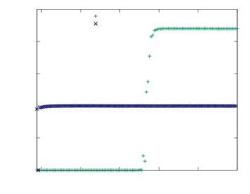
The impact of the small size of the energy space of the $8\times 8$ Ising model becomes already clear by considering the $16\times 16$ Ising model. In Fig. 4, the behavior of the deviation from the exact solution of the DOS obtained by the SAMC algorithm for the $16\times 16$ Ising model is depicted for different $t_{0}$ on the left. The flatness of the histogram for those values of $t_{0}$ is shown on the right. For $t_{0}=100$, the algorithm fails to generate a flat histogram in the simulation time of $10^{10}$ update attempts. The final histogram of that simulation is shown in Fig. 5. The states below $E\approx-200$ are almost never visited.

Figure 6: The behavior of the average deviation from the exact solution $\langle\epsilon(t)\rangle_{E}$ over MC time $t$ for SAMC for different $t_{0}$ and $1/t$-WL simulations of the $32\times 32$ (left) and $64\times 64$ (right) Ising model. The $1/t$-WL simulations converge faster than all SAMC simulations in both cases.

Figure 7: The behavior of the deviation $\langle\epsilon\rangle$ of the simulated DOSes from SAMC and $1/t$-WL simulations for various (larger) lattice sizes. $t_{0}$ was chosen as $t_{0}=100L^{2}$ for all SAMC simulations in order to check the rule of thumb given by Liang et al. [9]. The time axis is given in sweeps ($1\text{ sweep}\equiv L^{2}$ updates) here to allow a comparison between the different lattice sizes.

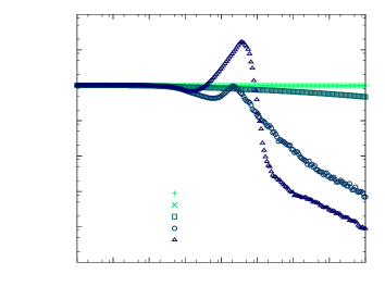
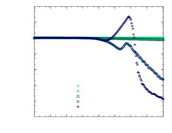
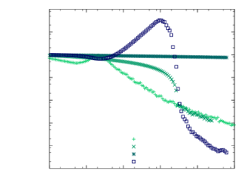
This is also reflected in the DOS failing to converge, the deviation stays roughly at one for the whole simulation time. For $t_{0}=1000$ the behavior looks similar to that for $t_{0}=100$ in the $8\times 8$ Ising case, first converging slowly, then, after a steep decline of the deviation, transitioning into the $\langle\epsilon\rangle\propto t^{-1/2}$ behavior. For higher $t_{0}$, the histogram steadily flattens, then converges in the $\langle\epsilon\rangle\propto t^{-1/2}$ manner. This shows that the choice of an appropriate $t_{0}$ is crucial. In their original work [9], Liang et al. state that a rule of thumb for choosing an appropriate $t_{0}$ is between $2N_{E}$ and $100N_{E}$, where $N_{E}$ is the number of energy subregions. In our case, this is equal to the number of histogram bins. For the $16\times 16$ Ising model, we have $N_{E}=128$. Our finding that $t_{0}=100$ is too small, whereas $t_{0}=1000$ suffices, is in good agreement with this rule. The problem of choosing $t_{0}$ appropriately is avoided in the $1/t$-WL algorithm. This algorithm determines the starting point of the $1/t$-behavior by checking the sequence $F_{t}$ itself by comparing it to the desired $F_{t}\propto 1/t$ sequence. This procedure is more self-contained than the procedure used by SAMC, but has to rely on stochastic quantities (here the number of visits in each histogram bin) and an a-priori knowledge of the number of accessible energies which may be a problem for more complicated models [18, 11, 21]. This makes it hard to predict the runtime of the algorithm. The convergence of the $1/t$-algorithm in this example seems to be very good, even exceeding our best choice of $t_{0}$ for SAMC. This is visible in the left of Fig. 4.

6.3 Larger lattice sizes

For larger lattice sizes the necessity of choosing an appropriate value for $t_{0}$ becomes even more apparent. This is visible in Fig. 6, where the deviation from the exact solution during SAMC and $1/t$-WL simulations of the $32\times 32$ and $64\times 64$ Ising model is depicted. As expected, the time needed to explore the energy landscape increases with the lattice size (which is, of course, equivalent to increasing phase space size). If $t_{0}$ is chosen too small in the SAMC simulations, the algorithm fails to converge in our simulation time of $10^{10}$ updates. The $1/t$-WL algorithm, on the other hand, adapts to this increase by its flatness criterion which forces the algorithm to take all energies into account. This is visible in the figure by a rapid decrease of $\langle\epsilon\rangle$ when the $F\rightarrow F/2$ stage of the algorithm starts. Finally, the $F_{t}\propto 1/t$ behavior sets in and the deviation $\langle\epsilon\rangle$ decreases like $t^{-1/2}$. While the $1/t$-WL algorithm manages to find the right time for the onset of the $1/t$-stage by itself in case of the Ising model, for SAMC it is up to the user to decide which $t_{0}$ is sufficiently large to ensure convergence. Our simulations for the quite uncomplicated Ising model already give a hint that this might be an intricate task for more difficult models. In Fig. 7, we show that the rule of thumb mentioned in Section 6.2 is no longer applicable for the $128\times 128$ Ising model: All SAMC simulations shown in this figure were carried out using $t_{0}=100L^{2}$, which is even larger than the value of $100N_{E}$ given by the rule of thumb. While still converging for the $32\times 32$ and $64\times 64$ models, the algorithm fails to reduce $\langle\epsilon\rangle$ within $10^{7}$ sweeps for the $128\times 128$ model. Additionally, we show the performance of the $1/t$-WL algorithm for the $128\times 128$ Ising model, which again outperforms the SAMC variants in terms of faster convergence.

6.4 Thermodynamic quantities of the Ising model obtained by SAMC

Figure 8: The internal energy $u$ per spin (left) and the specific heat $c$ per spin (right) for the $16\times 16$ Ising model depending on inverse temperature $\beta$ compared to data obtained from the exact Beale solution. The two curves coincide. The insets show the relative deviations $\epsilon$ of the internal energy and specific heat from the exact solution.

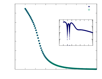
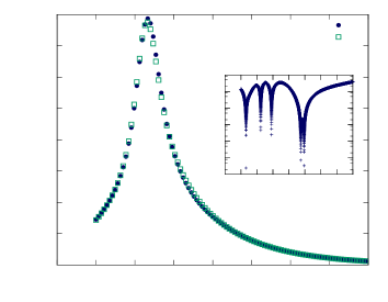
The estimators for the DOS obtained in the SAMC simulation were used to obtain an estimate of the internal energy $u$ and the specific heat $c$ per lattice site of the $16\times 16$ Ising model. The estimators for $u$ and $c$ were obtained by using the fact that for arbitrary inverse temperatures $\beta$ we can calculate $\widehat{u}(\beta)=\widehat{U}(\beta)/V$ and $\widehat{c}(\beta)=\widehat{C}(\beta)/V$ from the DOS by

$$\widehat{U}(\beta) =\widehat{\langle E\rangle}=\frac{\sum_{E}E\;\widehat{g}(E)e^{-\beta E}}{\sum_{E}\widehat{g}(E)e^{-\beta E}}=\frac{\sum_{E}Ee^{S(E)-\beta E}}{\sum_{E}e^{S(E)-\beta E}}\;,$$ (6)

$$\widehat{C}(\beta) =\beta^{2}(\widehat{\langle E^{2}\rangle}-\widehat{\langle E\rangle}^{2})=\beta^{2}\left(\frac{\sum_{E}E^{2}e^{S(E)-\beta E}}{\sum_{E}e^{S(E)-\beta E}}-\widehat{\langle E\rangle}^{2}\right)\;.$$

In Fig. 8 the curves obtained by this method are shown compared to the exact curves from plugging Beale’s solution into Eq. (6). The simulation parameters were $t_{0}=1000$ and the total MC time was $10^{10}$. By the naked eye, for the internal energy no differences can be spotted. In the insets we show the relative deviations of the two curves which is very small for the internal energy and small for the specific heat.

These results show that, if a run of SAMC has converged, its results can be used for accurate calculations of thermodynamic properties of physical models. Nevertheless, this procedure is not advisable for more complex systems, because it does not allow a straightforward calculation of the errors of the obtained physical quantities, since the error of the DOS is generally not known. Therefore a multicanonical [22, 23, 24] production run using the inverse of the obtained estimator of the DOS as weights is highly recommended. Moreover, a subsequent production run can single out runs of the SAMC algorithm which have not converged. The data from Section 6 shows that this can be a serious issue even for the Ising model, depending on the choice of $t_{0}$.

7 Conclusion

The error saturation in the Wang-Landau algorithm found in Refs. [5] and [6] was reproduced. A possible cure for this is to use an alternative behavior of the refinement parameter as is done in the $1/t$-WL and SAMC algorithms. The $1/t$-method inherits the problem from the Wang-Landau algorithm of needing to know the range of admissible energies for the considered model. In SAMC, this needs not to be known beforehand, since histogram checking is not necessary in principle. The SAMC algorithm, on the other hand, sometimes failed to converge in our examined runtimes. This is caused by the simulation failing to explore the low-energy states. Therefore no flat histogram can be produced. Since both variants of the Wang-Landau algorithm regularly check the histogram for adequate flatness, it is ensured that all energies are visited at least once. While the SAMC algorithm should converge to the desired distribution if all conditions are met, it is necessary to check if the histogram measured during the simulation was really flat at the end. This dampens the advantage of a predictable runtime, since it is possible that a complete run of the algorithm turns out to be unusable due to an inappropriate choice of $t_{0}$. Monitoring the flatness of the histogram during the run is no help, because this would introduce a stochastic quantity into the algorithm, making the runtime unpredictable and require the same a-priori knowledge of the admissible energy range as the Wang-Landau algorithm and its modifications. The rule of thumb for the choice of $t_{0}$ given by Liang et al. [9] is violated even by the $128\times 128$ Ising model, showing that finding an appropriate $t_{0}$ can be a quite cumbersome task. The $1/t$-WL algorithm suffers from a similar restriction in this regard: While we could not find anything comparable in the Ising model, other studies suggest that the overall convergence behavior can also be sensitive to the details of the $1/t$-refining scheme for more complicated models [7, 11]. Regarding the common features of the SAMC and $1/t$-WL algorithms, it seems reasonable to assume that the proof of convergence for SAMC also extends to the $1/t$-WL algorithm as well, since their long-time behavior is the same. Therefore the choice of algorithm to apply to a certain problem is a practical one. With the modifications proposed in Refs. [18, 11], allowing it to adapt to a-priori unknown energy ranges, and in Refs. [7, 11], allowing it to find the right time for the onset of the $1/t$-refinement, the $1/t$-WL algorithm might be able to overcome its drawback for complicated systems with unknown ground states. SAMC still has the advantage of allowing to generate weights not only according to the density of states, but also according to other distributions [8, 9], which can improve estimators [20] and might prove useful for complex systems like spin glasses or polymers, because sampling with distributions other than the inverse density of states can speed up round trip times significantly [25].

References

- Wang and Landau [2001a] F. Wang, D. P. Landau, Phys. Rev. Lett. 86 (2001a) 2050.
- Wang and Landau [2001b] F. Wang, D. P. Landau, Phys. Rev. E 64 (2001b) 056101.
- Janke and Paul [2016] W. Janke, W. Paul, Soft Matter 12 (2016) 642.
- Yan and de Pablo [2003] Q. Yan, J. J. de Pablo, Phys. Rev. Lett. 90 (2003) 035701.
- Belardinelli and Pereyra [2007a] R. E. Belardinelli, V. D. Pereyra, J. Chem. Phys. 127 (2007a) 184105.
- Belardinelli and Pereyra [2007b] R. E. Belardinelli, V. D. Pereyra, Phys. Rev. E 75 (2007b) 046701.
- Zhou and Su [2008] C. Zhou, J. Su, Phys. Rev. E 78 (2008) 046705.
- Liang [2006] F. Liang, J. Stat. Phys. 122 (2006) 511.
- Liang et al. [2007] F. Liang, C. Liu, R. J. Carroll, J. Amer. Statist. Assoc. 102 (2007) 305.
- Belardinelli et al. [2008] R. Belardinelli, S. Manzi, V. Pereyra, Phys. Rev. E 78 (2008) 067701.
- Swetnam and Allen [2011] A. D. Swetnam, M. P. Allen, J. Comput. Chem. 32 (2011) 816.
- Werlich et al. [2015] B. Werlich, T. Shakirov, M. P. Taylor, W. Paul, Comput. Phys. Commun. 186 (2015) 65.
- Ising [1925] E. Ising, Z. Phys. 31 (1925) 253.
- Onsager [1944] L. Onsager, Phys. Rev. 65 (1944) 117.
- Kaufman [1949] B. Kaufman, Phys. Rev. 76 (1949) 1232.
- Beale [1996] P. D. Beale, Phys. Rev. Lett. 76 (1996) 78.
- Schierz et al. [2016] P. Schierz, J. Zierenberg, W. Janke, Phys. Rev. E 94 (2016) 021301(R).
- Wüst and Landau [2009] T. Wüst, D. P. Landau, Phys. Rev. Lett. 102 (2009) 178101.
- Andrieu et al. [2005] C. Andrieu, É. Moulines, P. Priouret, SIAM J. Control Optim. 44 (2005) 283.
- Hesselbo and Stinchcombe [1995] B. Hesselbo, R. B. Stinchcombe, Phys. Rev. Lett. 74 (1995) 2151.
- Wüst and Landau [2012] T. Wüst, D. P. Landau, J. Chem. Phys 137 (2012) 064903.
- Berg and Neuhaus [1991] B. A. Berg, T. Neuhaus, Phys. Lett. B 267 (1991) 249.
- Berg and Neuhaus [1992] B. A. Berg, T. Neuhaus, Phys. Rev. Lett. 68 (1992) 9.
- Janke [1992] W. Janke, Int. J. Mod. Phys. C 3 (1992) 1137.
- Trebst et al. [2004] S. Trebst, D. A. Huse, M. Troyer, Phys. Rev. E 70 (2004) 046701.