Dimension reduction via $\Gamma$-convergence
for soft active materials

Abstract.

We present a rigorous derivation of dimensionally reduced theories for thin sheets of nematic elastomers, in the finite bending regime. Focusing on the case of twist nematic texture, we obtain 2D and 1D models for wide and narrow ribbons exhibiting spontaneous flexure and torsion. We also discuss some variants to the case of twist nematic texture, which lead to 2D models with different target curvature tensors. In particular, we analyse cases where the nematic texture leads to zero or positive Gaussian target curvature, and the case of bilayers.

1. Introduction

We discuss in this paper some recent (and some new) results motivated by shape programming problems for thin structures, made of soft active materials. In particular, we focus our attention on nematic elastomers [1, 2, 5, 14, 15, 28]. These are polymeric materials that, thanks to the coupling between elasticity and orientational nematic order, undergo spontaneous deformations as a consequence of a temperature-driven phase transformation.

When a nematic texture (i.e. a spatially-dependent orientation of the nematic director) is present, non-uniform spontaneous strains lead to stress build-up and non-trivial configurational changes. Here, we explore in particular the consequences of through-the-thickness changes of orientation in thin sheets. Plates with spontaneous and controllable curvature emerge in this way. When the plate is in the form of a narrow ribbon, rods with spontaneous flexure and torsion are generated. Similar issues have been the object of recent intense investigation, see e.g. [3, 6, 22, 23, 27] and also [7, 9, 10, 12, 13, 19, 25]. The point of view we adopt here is that of a systematic derivation of dimensionally-reduced models by means of $\Gamma$-convergence. Far from being just a technical exercise, this technique allows one to derive, rather than postulate, the functional form and the material parameters (elastic constants, spontaneous curvature, etc.) for dimensionally reduced models of these structures.

Building upon our recent work [3, 6], which has been in turn inspired by [17, 18, 24], we discuss in this paper the derivation of models capable of describing non-trivial shapes that can be spontaneously exhibited by thin sheets of nematic elastomers. In particular, we focus on the twist director geometry, and we present a derivation of reduced models for wide and narrow ribbons (namely, rods whose cross-section is a thin rectangle) by following a sequential dimension reduction technique, namely, a 3D$\rightarrow$2D$\rightarrow$1D procedure, see Section 2. Plates made of twist nematic elastomers spontaneously deform into cylindrical ribbons. This geometry emerges as a “compromise” between the energetic drive towards a non-zero target curvature (with negative Gaussian curvature) and an isometry constraint on the mid-surface (which rules out surfaces with non-zero Gaussian curvature). Narrow ribbons obtained from rectangular plates of vanishing small width behave as rods with spontaneous flexure and torsion.

Moreover, we also consider in Section 3 some alternative scenarios to the case of twist nematic texture, in which the target curvature tensor of the 2D reduced model has either zero or positive Gaussian curvature. Nematic textures realising these possibilities are the splay-bend one and uniform director alignment perpendicular to the mid-plane, respectively. Alternatively, the three alternative scenarios (positive, negative, or zero Gaussian curvature of the target curvature tensor in the 2D plate theory) can be realised in bilayers, by tuning the spontaneous strains in the two halves of the bilayer. In all these cases, configurations with non-zero Gaussian curvature are again frustrated by the isometry constraint. Hence, the configurations that are spontaneously exhibited are always ribbons wrapped around cylinders. Much of the material relating to nematic elastomer sheets draws on our analyses contained in [3, 6], but it is presented here from the unifying perspective of a sequential dimensional reduction, first from three to two dimensions, and then from two to one dimension. The analysis of thin bilayer sheets is new. We refer the reader to [20] for a discussion of bilayer beams.

2. Wide and narrow ribbons of nematic elastomers

In this section, we consider a thin sheet of nematic elastomer with twist distribution of the director along the thickness. Starting from a $3D$ model, described in Subsection 2.1, we present in Subsection 2.2 the rigorous derivation of a corresponding $2D$ plate model. In Subsection 2.3 we then derive, again via $\Gamma$-convergence arguments, a $1D$ rod model from the $2D$ model.

Before proceeding, let us establish some general notation which will be used throughout. For the standard basis of $\mathbb{R}^{3}$ and $\mathbb{R}^{2}$, we use the notation $\{\mathsf{e}_{1},\mathsf{e}_{2},\mathsf{e}_{3}\}$ and $\{\mathsf{f}_{1},\mathsf{f}_{2}\}$, respectively. ${\rm SO}(3)$ and ${\rm Sym}(3)$ are the sets of $3{\times 3}$ rotations and symmetric matrixes, respectively, and ${\rm I}\in{\rm SO}(3)$ is the identity matrix. We use the symbol ${\rm tr}^{2}A$ for the square of the trace of a matrix $A$, and denote by $\mathbb{S}^{2}$ the unit sphere of $\mathbb{R}^{3}$. Finally, the symbol $C$ will be used to denote a positive constant depending on given data, and possibly varying from line to line.

2.1. The three-dimensional model

We consider a thin sheet of nematic elastomer occupying the reference configuration

$$\Omega_{h}^{\varepsilon}\,:=\,\Omega_{h}^{\varepsilon}(\theta)\,:=\,\bigg{\{}z_{1}\mathsf{e}_{1}^{\theta}+z_{2}\mathsf{e}_{2}^{\theta}+z_{3}\mathsf{e}_{3}\,:\,z_{1}\in\big{(}-\ell/2,\ell/2\big{)},\ z_{2}\in\big{(}-\varepsilon/2,\varepsilon/2\big{)},\ z_{3}\in\big{(}-h/2,h/2\big{)}\bigg{\}},$$

where

$$\mathsf{e}_{1}^{\theta}\,:=\,\left(\begin{array}[]{c}\cos\theta\\ \sin\theta\\ 0\end{array}\right)\qquad\quad\mbox{and}\qquad\quad\mathsf{e}_{2}^{\theta}\,:=\,\left(\begin{array}[]{c}-\sin\theta\\ \cos\theta\\ 0\end{array}\right),$$

and $\varepsilon>0$ and $h>0$ are small dimensionless parameters such that

$$\ell\gg\varepsilon\gg h.$$

The directions $\mathsf{e}_{1}$ and $\mathsf{e}_{2}$ play a special role, which is related to the orientation of the nematic director on the top and bottom faces of the thin sheet, see (2.3) below and Figure 1. For future reference, we also set $\Omega_{h}^{\varepsilon}:=\omega^{\varepsilon}\times(-h/2,h/2)$, with

$$\omega^{\varepsilon}\,=\,\omega^{\varepsilon}(\theta)\,:=\,\bigg{\{}z_{1}\mathsf{f}_{1}^{\theta}+z_{2}\mathsf{f}_{2}^{\theta}\,:\,z_{1}\in\big{(}-\ell/2,\ell/2\big{)},\ z_{2}\in\big{(}-\varepsilon/2,\varepsilon/2\big{)}\bigg{\}},$$ (2.1)

and

$$\mathsf{f}_{i}^{\theta}\,:=\,R_{\theta}\mathsf{f}_{i},\quad\ i=1,2,\qquad\quad R_{\theta}\,:=\,\left(\begin{array}[]{cc}\cos\theta&-\sin\theta\\ \sin\theta&\cos\theta\\ \end{array}\right),\qquad\quad 0\leq\theta<\pi.$$ (2.2)

Our nematic elastomer thin sheet will be modelled by a stored energy density which is heterogeneous along the thickness. More precisely, in the model we are going to consider, the nematic director varies along the thickness. This will induce a $z_{3}$-dependence of the spontaneous strain distributions and, in turn, $z_{3}$-dependent stored energy densities. The system under analysis is a twist nematic elastomer thin sheet. The distribution of the nematic director in the twist geometry is defined as

$$\hat{n}_{h}(z_{3})\,:=\,\left(\begin{array}[]{c}\cos\big{(}\frac{\pi}{4}+\frac{\pi}{2}\frac{z_{3}}{h}\big{)}\\ \sin\big{(}\frac{\pi}{4}+\frac{\pi}{2}\frac{z_{3}}{h}\big{)}\\ 0\end{array}\right),\qquad\qquad z_{3}\in\Big{[}-\frac{h}{2},\frac{h}{2}\,\Big{]},$$ (2.3)

see Figure 1. Note that this distribution is constant on each horizontal plane and in particular $n_{h}$ is (constantly) equal to $\mathsf{e}_{1}$ and to to $\mathsf{e}_{2}$ on the bottom and on the top face of the sheet, respectively. Also, recall that such distribution is the ($\varepsilon$-independent) solution to the minimum problem

$$\min_{\begin{array}[]{r}n(-h/2)=\mathsf{e}_{1}\\ n(h/2)=\mathsf{e}_{2}\end{array}}\int\limits_{\Omega_{h}^{\varepsilon}}|\nabla n|^{2}{\rm d}z.$$

This is the orientation arising in the fabrication procedure of the material, in which the director is oriented in the liquid phase, and then “frozen” by the crosslinking process transforming the liquid into an elastomer.

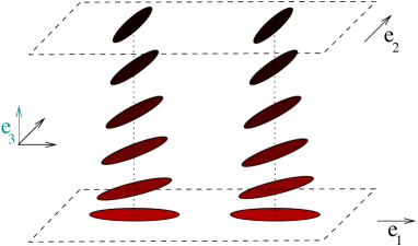
Figure 1. Sketch of the twist director field.

Now, if $n\in\mathbb{R}^{3}$ is a unit vector representing the local order of the nematic director, the (local) response of the nematic elastomer is encoded by the positive definite symmetric matrix

$$L(n)=a^{\frac{2}{3}}n\otimes n+a^{-\frac{1}{3}}({\rm I}-n\otimes n),$$ (2.4)

where $a>1$ is a material parameter. More precisely, under the effect of lowering the temperature below a threshold (isotropic-to-nematic transition temperature), in a region where the nematic director is $n$, the material spontaneously deforms via a deformation $y$ such that $\nabla y^{T}\nabla y~{}=~{}L(n)$. As a consequence, the through-the-thickness variation of the nematic director translates into the spontaneous strain field

$$\widehat{C}_{h}(z_{3})\,:=\,L(\hat{n}_{h}(z_{3}))\,=\,a_{h}^{2/3}\hat{n}_{h}(z_{3})\otimes\hat{n}_{h}(z_{3})+a_{h}^{-1/3}\big{(}{\rm I}-\hat{n}_{h}(z_{3})\otimes\hat{n}_{h}(z_{3})\big{)}.$$ (2.5)

Notice that, in this expression, we allow the material parameter $a$ to be $h$-dependent. More precisely, from now on we will assume that

$$a_{h}=1+\frac{\alpha_{0}}{h_{0}}h,$$ (2.6)

where $\alpha_{0}$ is a positive dimensionless parameter, while $h_{0}$ and $h$ have the physical dimension of length. This assumption is easily understandable if one thinks that, arguing as in the proof of the Gauss Lemma (see, e.g., [21, Chapter 5]), a given metric $g$ of $\mathbb{R}^{3}$ can always be expressed around a smooth hypersurface $\Sigma$ as

$$g\,=\,dr\otimes dr+g_{ij}d\theta^{i}\otimes d\theta^{j},$$

using coordinates $\{r,\theta^{1},\theta^{2}\}$, where $r$ is the signed $g$-distance from $\Sigma$. In the coordinates $\{\theta^{1},\theta^{2}\}$, one can then express the second fundamental form ${\rm A}$ on $\Sigma$ as

$${\rm A}_{ij}\,d\theta^{i}\otimes d\theta^{j}\,=\,\frac{1}{2}\frac{\partial g_{ij}}{\partial r}\,d\theta^{i}\otimes d\theta^{j}.$$

In other words, via the standard identification of metric and strain, curvature is related to the ratio between the magnitude of the strain difference along the thickness and the thickness itself. Hence, the linear scaling in $h$ in (2.6) is needed in order to obtain a finite curvature in the limit $h\to 0$.

To model our system in the framework of finite elasticity, we consider the energy density $\widehat{W}_{h}$ defined on points of $(-h/2,h/2){\times}\mathbb{R}^{3{\times}3}$ as

$$\widehat{W}_{h}(z_{3},F):=\left\{\begin{array}[]{ll}\displaystyle\frac{\mu}{2}\Big{[}(F^{T}F)\cdot\widehat{C}_{h}^{-1}(z_{3})-3-2\log(\det F)\Big{]}+W_{vol}(\det F)&\quad\mbox{if }\det F>0,\\ +\infty&\quad\mbox{if }\det F\leq 0,\end{array}\right.$$ (2.7)

which also accounts for compressibility effects. Here, $\mu>0$ is a material constant (shear modulus) and the function $W_{vol}:(0,\infty)\to[0,\infty)$ is ${\rm C}^{2}$ around $1$ and fulfills the conditions:

$$W_{vol}(t)=0\iff t=1,\qquad W_{vol}(t)\longrightarrow\infty\ \,{\rm as}\ \,t\to 0^{+},\qquad W_{vol}^{\prime\prime}(1)>0.$$

A typical example of $W_{vol}$ is $t\mapsto c\,(t^{2}-1-2\log t)$, where $t$ is nondimensional and $c$, a positive constant, is energy per unit volume, so that $W_{vol}^{\prime\prime}(1)$ has the same dimension of $\mu$. Expression (2.7) is a natural generalization, see [4], of the classical trace formula for nematic elastomers derived by Bladon, Terentjev and Warner [10], in the spirit of Flory’s work on polymer elasticity [16]. The presence of the purely volumetric term $W_{vol}(\det F)$ guarantees that the Taylor expansion at order two of the density results in isotropic elasticity with two independent elastic constants (shear modulus and bulk modulus).

Observe that, for every $F$ with $\det F>0$,

$$\widehat{W}_{h}(z_{3},F)\,=\,W_{0}\big{(}F\widehat{U}_{h}(z_{3})^{-1}\big{)},\qquad\widehat{U}_{h}(z_{3})\,:=\,\widehat{C}_{h}(z_{3})^{\frac{1}{2}},$$ (2.8)

where

$$W_{0}(F)\,:=\,\frac{\mu}{2}\Big{[}|F|^{2}-3-2\log(\det F\,)\Big{]}+W_{vol}(\det F\,).$$ (2.9)

Also, note that

$$W_{0}(F)\,\geq\,\frac{\mu}{2}\Big{[}|F|^{2}-3-2\log(\det F\,)\Big{]}\,\geq\,\frac{3}{2}\mu\big{[}(\det F)^{\frac{2}{3}}-1-\log(\det F)^{\frac{2}{3}}\big{]}\,\geq\,0,$$

where in the second inequality we have used that $|F|^{2}\geq 3(\det F)^{\frac{2}{3}}$, due to the inequality between arithmetic and geometric mean, and the third inequality comes from direct computations. Also, the second and the third inequalities become equalities iff $F^{T}F=\alpha{\rm I}$, for some $\alpha\geq 0$, and iff $\det F=1$, respectively. All in all, we have that $W_{0}$ is a nonnegative function minimised precisely at ${\rm SO}(3)$. In turn, from (2.8), we have that $\widehat{W}_{h}(z_{3},\cdot)$ is a nonnegative function minimised precisely at ${\rm SO}(3)\widehat{C}(z_{3})^{\frac{1}{2}}$. Let us also point out that from the expression of the second differential ${\rm D}^{2}W_{0}({\rm I})$ of $W_{0}$ at ${\rm I}$ applied twice to some $M\in\mathbb{R}^{3\times 3}$, namely

$$Q_{3}(M)\,:=\,{\rm D}^{2}W_{0}({\rm I})[M,M]\,=\,2\mu\,|{\rm sym}\,M|^{2}+W_{vol}^{\prime\prime}(1)\,{\rm tr}^{2}M,$$ (2.10)

and from the fact that $W_{0}(F)\geq C|F|^{2}$ for $|F|\gg 0$, one can easily deduce that

$$W_{0}(F)\,\geq\,C{\rm dist}^{2}(F,{\rm SO}(3)),\qquad\quad\mbox{for all}\ F\in\mathbb{R}^{3}.$$ (2.11)

This is one of the sufficient conditions which allow us to apply the results of [24], in the next subsection. Note that the quadratic growth of $W_{0}$ from ${\rm SO}(3)$ implies that

$$\widehat{W}_{h}(z_{3},F)\,\geq\,C{\rm dist}^{2}\big{(}F\widehat{U}_{h}(z_{3})^{-1},{\rm SO}(3)\big{)}\,\geq\,C\lambda_{min}^{2}(z_{3}){\rm dist}^{2}\big{(}F,{\rm SO}(3)\widehat{U}_{h}(z_{3})\big{)},\qquad\quad\mbox{for all}\ F\in\mathbb{R}^{3},$$

where $\lambda_{min}(z_{3})>0$ is the minimum eigenvalue of $\widehat{U}_{h}(z_{3})$. Also, observe from (2.10) that while $\mu$ is the elastic shear modulus, $W_{vol}^{\prime\prime}(1)+2\mu/3$ has the physical meaning of bulk modulus.

We denote by $\widehat{\mathscr{F}}_{h}^{\varepsilon}$ the free-energy functional corresponding to the energy density $\widehat{W}_{h}$, i.e.

$$\widehat{\mathscr{F}}_{h}^{\varepsilon}(v)\,:=\,\int\limits_{\Omega_{h}^{\varepsilon}}\widehat{W}_{h}(z_{3},\nabla v(z))\,{\rm d}z,$$ (2.12)

where $v:\Omega_{h}^{\varepsilon}\to\mathbb{R}^{3}$ is a deformation and $z=(z^{\prime},z_{3})$ is a point of $\Omega_{h}^{\varepsilon}$, whose components are given w.r.t.  the canonical basis $\{\mathsf{e}_{1},\mathsf{e}_{2},\mathsf{e}_{3}\}$.

2.2. The plate model

In order to derive rigorously, in the limit as $h\downarrow 0$, a 2D model from the 3D setting, we first make a standard change of variables which allows us to rewrite the energies in a fixed, $h$-independent rescaled reference configuration. We denote by $x=(x_{1},x_{2},x_{3})=(x^{\prime},x_{3})$ an arbitrary point in the rescaled reference configuration $\Omega^{\varepsilon}:=\omega^{\varepsilon}\times(-1/2,1/2)$. For every $h>0$ small, we define the rescaled energy density $W_{h}:(-1/2,1/2)\times\mathbb{R}^{3\times 3}\longrightarrow[0,+\infty]$ as

$$W_{h}(x_{3},F)\,:=\,\widehat{W}_{h}(hx_{3},F).$$ (2.13)

Note that $W_{h}$ fulfills

$$W_{h}(x_{3},F)=0\qquad\quad\mbox{iff}\qquad\quad F\in{\rm SO}(3)\overline{U}_{h}(x_{3}),\qquad\qquad\overline{U}_{h}(x_{3}):=\widehat{U}_{h}(hx_{3}).$$

We also set $\overline{C}_{h}(x_{3}):=\overline{U}_{h}^{2}(x_{3})$. Finally, defining

$$\nabla_{h}y:=\left(\begin{array}[]{ccccc}\!\!\partial_{x_{1}}y\!\!&\!\!\bigg{|}\!\!&\!\!\partial_{x_{2}}y\!\!&\!\!\bigg{|}\!\!&\!\!\displaystyle\frac{\partial_{x_{3}}y}{h}\!\!\end{array}\right)=:\left(\begin{array}[]{ccccc}\!\!\nabla^{\prime}y\!\!&\!\!\bigg{|}\!\!&\!\!\displaystyle\frac{\partial_{x_{3}}y}{h}\!\!\end{array}\right),\qquad\qquad\mbox{for every}\quad y:\Omega^{\varepsilon}\longrightarrow\mathbb{R}^{3},$$ (2.14)

the correspondence between the original quantities and the rescaled ones is through the formulas

$$\widehat{\mathscr{F}}_{h}^{\varepsilon}(v)\,=\,h\,\mathscr{F}_{h}^{\varepsilon}(y),\qquad\qquad v(z):=y(z^{\prime},z_{3}/h)\quad\mbox{for a.e.}\ z\in\Omega_{h}^{\varepsilon}.$$ (2.15)

Here, the rescaled free-energy functional $\mathscr{F}_{h}^{\varepsilon}$ is defined, on a deformation $y:\Omega^{\varepsilon}\to\mathbb{R}$, as

$$\mathscr{F}_{h}^{\varepsilon}(y)\,:=\,\int\limits_{\Omega^{\varepsilon}}W_{h}(x_{3},\nabla_{h}y(x))\,{\rm d}x.$$

To deal with the (rescaled) spontaneous strains $\overline{C}_{h}(x_{3})$, we first note that the rescaled director field has the following expression:

$$n(x_{3}):=\hat{n}_{h}(hx_{3})=\left(\begin{array}[]{c}\cos\big{(}\frac{\pi}{4}+\frac{\pi}{2}x_{3}\big{)}\\ \sin\big{(}\frac{\pi}{4}+\frac{\pi}{2}x_{3}\big{)}\\ 0\end{array}\right)\!,$$ (2.16)

which is independent of $h$. In turn, we obtain for $\overline{C}_{h}(x_{3})$ the equivalent expression

$$\overline{C}_{h}(x_{3}) =a_{h}^{2/3}n(x_{3})\otimes n(x_{3})+a_{h}^{-1/3}\big{(}{\rm I}-n(x_{3})\otimes n(x_{3})\big{)}$$

$$=\big{(}a_{h}^{2/3}-a_{h}^{-1/3}\big{)}\left(\frac{\rm I}{a_{h}-1}+n(x_{3})\otimes n(x_{3})\right)$$

$$={\rm I}-2\,h\,B(x_{3})+R^{h}(x_{3}),\qquad\quad B(x_{3})\,:=\,\frac{1}{2}\frac{\alpha_{0}}{h_{0}}\left(\frac{\rm I}{3}-n(x_{3})\otimes n(x_{3})\right),$$ (2.17)

where $\|R^{h}\|_{\infty}=o(h)$ and $\|\cdot\|_{\infty}$ is the norm in the space ${\rm L}^{\infty}\big{(}(-1/2,1/2),\mathbb{R}^{3\times 3}\big{)}$. Note that in the third equality we have plugged in expression (2.6) for $a_{h}$ and used the expansion

$$a_{h}^{2/3}-a_{h}^{-1/3}=\frac{\alpha_{0}}{h_{0}}h-\frac{1}{3}\left(\frac{\alpha_{0}}{h_{0}}\right)^{2}h^{2}+o(h^{2}).$$

Moreover, plugging into (2.2) the expression for $n$ given by (2.16), we have that

$$B(x_{3})\,=\,\frac{1}{2}\frac{\alpha_{0}}{h_{0}}\left(\begin{array}[]{ccc}\frac{1}{3}-\cos^{2}\big{(}\frac{\pi}{4}+\frac{\pi}{2}x_{3}\big{)}&\frac{1}{2}\sin\big{(}\frac{\pi}{2}+\pi x_{3}\big{)}&0\\ \frac{1}{2}\sin\big{(}\frac{\pi}{2}+\pi x_{3}\big{)}&\frac{1}{3}-\sin^{2}\big{(}\frac{\pi}{4}+\frac{\pi}{2}x_{3}\big{)}&0\\ 0&0&\frac{1}{3}\\ \end{array}\right).$$ (2.18)

The description of the 3D system provided by (2.8), (2.13), and (2.2) allows us to directly use the results of [24] for the derivation of a corresponding limiting model, in the regime of finite bending energies. More precisely, in [3] we can state a compactness result for sequences $\{y_{h}\}$ such that $\mathscr{F}_{h}^{\varepsilon}(y_{h})\leq Ch^{2}$, and a $\Gamma$-convergence result for $\mathscr{F}_{h}^{\varepsilon}/h^{2}$, in the limit $h\downarrow 0$. In particular, we can compute the limiting 2D model. In order to do it, we first compute, for every $G\in\mathbb{R}^{2\times 2}$, the relaxed energy density

$$Q_{2}(G)\,:=\,\min_{\stackrel{{\scriptstyle b\in\mathbb{R}^{2}}}{{a\in\mathbb{R}}}}Q_{3}\left(\left[\begin{tabular}[]{c|c}$G$&$b$\\ \hline\cr$0$&$a$\end{tabular}\right]\right)\,=\,2\mu\Big{(}\,|{\rm sym}\,G|^{2}+\gamma\,{\rm tr}^{2}G\Big{)},$$ (2.19)

where $Q_{3}$ is defined in (2.10) and

$$\gamma:=\frac{W_{vol}^{\prime\prime}(1)}{2\mu+W_{vol}^{\prime\prime}(1)}.$$ (2.20)

The adjective “relaxed” used for the two-dimensional energy density $Q_{2}$ is due to the fact that it arises from an optimisation procedure. Then, we compute the doubly relaxed energy density

$$\overline{Q}_{2}(G) \,:=\,\min_{D\in\mathbb{R}^{2\times 2}}\int\limits_{-1/2}^{1/2}Q_{2}\big{(}D+t\,G+\check{B}(t)\big{)}{\rm d}t$$ (2.21)

$$\,=\,\alpha_{T}\,Q_{2}(G-\bar{A}_{T})+\beta_{T},$$

where the $2{\times}2$ symmetric matrix $\check{B}$ is obtained from $B$ (cf. (2.2) and (2.18)) by omitting the last row and the last column, namely

$$\check{B}\,:=\,\sum_{ij=1}^{2}B_{ij}\,\mathsf{f}_{i}\otimes\mathsf{f}_{j}.$$ (2.22)

Moreover, the constants $\alpha_{T}$ (a geometric parameter, reminiscent of the “moment of inertia” of a cross section of unit width), $\bar{A}_{T}$ (the target curvature tensor), and $\beta_{T}$ (a positive constant, reminder of the presence of residual stresses, cf. Remark 2.2) are given by the formulas:

$$\alpha_{T}\,=\,\frac{1}{12},\quad\qquad\bar{A}_{T}\,=\,\frac{6}{\pi^{2}}\frac{\alpha_{0}}{h_{0}}\,{\rm diag(-1,1)},\quad\qquad\beta_{T}\,=\,\mu\,\Big{(}\frac{\pi^{4}-4\pi^{2}-48}{4\pi^{4}}\Big{)}\frac{\alpha_{0}^{2}}{h_{0}^{2}}.$$ (2.23)

The 2D free-energy limit functional turns out to have the following expression:

$$\mathscr{F}_{lim}^{\varepsilon}(y)\,:=\,\frac{1}{2}\int\limits_{\omega^{\varepsilon}}\left[\alpha_{T}\,Q_{2}(A_{y}(x^{\prime})-\bar{A}_{T})+\beta_{T}\right]{\rm d}x^{\prime},$$ (2.24)

if $y\in{\rm W}^{2,2}_{\rm iso}(\omega^{\varepsilon},\mathbb{R}^{3})$, while $\mathscr{F}_{lim}^{\varepsilon}(y)=+\infty$ elsewhere in ${\rm W}^{1,2}(\Omega^{\varepsilon},\mathbb{R}^{3})$. Here, the symbol $A_{y}(x^{\prime})$ stands for the second fundamental form associated with $y(\omega_{\varepsilon})$ and defined at points $x^{\prime}\in\omega_{\varepsilon}$, namely $A_{y}(x^{\prime}):=(\nabla^{\prime}y(x^{\prime}))^{T}\nabla^{\prime}\nu(x^{\prime})$, with $\nu:=\partial_{1}y\wedge\partial_{2}y$. Moreover, the class ${\rm W}^{2,2}_{\rm iso}(\omega^{\varepsilon},\mathbb{R}^{3})$ is that of the isometric immersions of $\omega^{\varepsilon}$ into the three-dimensional Euclidean space, namely

$${\rm W}^{2,2}_{\rm iso}(\omega^{\varepsilon},\mathbb{R}^{3})\,:=\,\Big{\{}y\in{\rm W}^{2,2}(\omega^{\varepsilon},\mathbb{R}^{3})\,:\,(\nabla^{\prime}y)^{T}\nabla^{\prime}y={\rm I}_{2}\ \mbox{\ }{a.e.\ in\ }\,\omega^{\varepsilon}\Big{\}},$$ (2.25)

where ${\rm I}_{2}$ is the identity matrix of $\mathbb{R}^{2\times 2}$.

The following theorem is a straightforward corollary of the aforementioned compactness and $\Gamma$-convergence results, for which we refer the reader to [3].

Theorem 2.1.

Setting

$$m_{h}:=\inf_{y\in{\rm W}^{1,2}}\mathscr{F}_{h}^{\varepsilon},$$

suppose that $\{y_{h}\}$ is a low-energy sequence, i.e. it fulfills

$$\lim_{h\to 0}\frac{\mathscr{F}_{h}^{\varepsilon}(y_{h})}{h^{2}}\,=\,\lim_{h\to 0}\frac{m_{h}}{h^{2}}.$$

Then, up to a subsequence, $y_{h}\longrightarrow y$ in ${\rm W}^{1,2}(\Omega^{\varepsilon},\mathbb{R}^{3})$, where $y\in{\rm W}^{2,2}_{\rm iso}(\omega^{\varepsilon},\mathbb{R}^{3})$ is a solution to the minimum problem

$$m_{lim}:=\min_{{\rm W}^{2,2}_{\rm iso}(\omega^{\varepsilon},\mathbb{R}^{3})}\mathscr{F}_{lim}^{\varepsilon}.$$

Moreover, $(m_{h}/h^{2})\to m_{lim}$.

Let us now fix a low-energy sequence $\{y_{h}\}$ converging to a minimiser $y\in{\rm W}^{2,2}_{\rm iso}(\omega^{\varepsilon},\mathbb{R}^{3})$ of the 2D model (2.24), and rephrase the theorem in terms of the physical quantities (2.12). Defining the deformations $v_{h}(z^{\prime},z_{3})=y_{h}(z^{\prime},z_{3}/h)$ in the physical reference configuration $\Omega_{h}$, we have $\lim_{h\to 0}\hat{\mathscr{F}}_{h}^{\varepsilon}(v_{h})/h^{3}=m_{lim}$, in view of (2.15). Equivalently, for a given small thickness $h_{0}$, the approximate identity

$$\hat{\mathscr{F}}_{T}^{h_{0}}(v_{h_{0}})\,\cong\,\frac{\mu\,h_{0}^{3}}{12}\int\limits_{\omega^{\varepsilon}}\left\{\bigg{|}{\rm A}_{y}(x^{\prime})-\frac{6}{\pi^{2}}\frac{\alpha_{0}}{h_{0}}\,{\rm diag(-1,1)}\bigg{|}^{2}+\gamma\,{\rm H}_{y}^{2}(x^{\prime})\right\}{\rm d}x^{\prime}\,+\,\mu\,h_{0}\,\alpha_{0}^{2}\Big{(}\frac{\pi^{4}-4\pi^{2}-48}{8\pi^{4}}\Big{)}|\omega^{\varepsilon}|$$

holds true, modulo terms of order higher than $3$ in $h_{0}$. Here, the symbol ${\rm H}_{y}$ denotes the mean curvature of $y(\omega^{\varepsilon})$, namely ${\rm H}_{y}={\rm tr}A_{y}$. In reading the formula, recall that the second fundamental form has physical dimension of inverse length.

Remark 2.2 (Kinematic incompatibility in 3D and geometric obstructions in 2D).

We remark that the spontaneous strain field $\Omega_{h}^{\varepsilon}\ni z\mapsto\widehat{C}(z)=\widehat{C}(z_{3})$ defined in (2.5) is not kinematically compatible, meaning that there are no smooth deformations $v:\Omega_{h}^{\varepsilon}\to\mathbb{R}^{3}$ such that, for every $z\in\Omega_{h}^{\varepsilon}$, $\det\nabla v(z)>0$ and

$$\nabla v^{T}\nabla v(z)=\widehat{C}(z_{3}).$$

To prove this fact, one can interpret $\widehat{C}$ as a given metric on $\Omega_{h}^{\varepsilon}$ and show equivalently (see [3] and [11]) that the fourth-order Riemann curvature tensor associated with the metric $\widehat{C}$ is not identically zero in $\Omega_{h}^{\varepsilon}$. This kinematic incompatibility and the related impossibility of minimising (to the value zero) the 3D energy functional (2.12), results into the presence of the positive constant $\beta_{T}$ in the 2D limiting model (2.23)–(2.24), which reveals the presence of residual stresses. Note at the same time that the quadratic term $Q_{2}(\cdot-\bar{A}_{T})$ in (2.24) per se prevents the attainment of zero as a minimum value of the energy. Indeed, there are no deformations $y$ in the class ${\rm W}^{2,2}_{\rm iso}(\omega^{\varepsilon},\mathbb{R}^{3})$ such that $y(\omega^{\varepsilon})$ has non-zero Gaussian curvature (while $\det\bar{A}_{T}<0$). More precisely, one can prove (see [3, Lemma 3.8]) that

$$\min_{{\rm W}^{2,2}_{\rm iso}(\omega^{\varepsilon},\mathbb{R}^{3})}\mathscr{F}^{lim}\,=\,\mathscr{F}^{lim}(y_{T})\,=\,\frac{3\,\mu}{\pi^{4}}\frac{\alpha_{0}^{2}}{h_{0}^{2}}\left(\frac{1+2\gamma}{1+\gamma}\right)|\omega^{\varepsilon}|+\frac{\beta_{T}}{2}|\omega^{\varepsilon}|,$$

where $y_{T}\in{\rm W}^{2,2}_{\rm iso}(\omega^{\varepsilon},\mathbb{R}^{3})$ is such that

$$\mbox{either}\qquad{\rm A}_{y_{T}}\equiv\frac{6}{\pi^{2}(1+\gamma)}\frac{\alpha_{0}}{h_{0}}{\rm diag}\left(-1,0\right)\qquad\mbox{or}\qquad{\rm A}_{y_{T}}\equiv\frac{6}{\pi^{2}(1+\gamma)}\frac{\alpha_{0}}{h_{0}}{\rm diag}\left(0,1\right).$$ (2.26)

Recall that $\omega^{\varepsilon}=\omega^{\varepsilon}(\theta)$ and therefore the minimisers $y_{T}$ are $\theta$-dependent in the sense that the long axis of the sheet ($\mathsf{f}_{1}^{\theta}$ in (2.1)) makes angles $\theta$ and $\pi/2-\theta$ with the eigenvectors $\mathsf{f}_{1}$ and $\mathsf{f}_{2}$ corresponding to the nonzero eigenvalue of the realised second fundamental forms (2.26), respectively.

2.3. The rod model

In this subsection, following [6], we derive a 1D reduced model, in the limit of vanishing width $\varepsilon\downarrow 0$, starting from the 2D setting (2.23)–(2.24). More precisely, the starting point of the following 1D derivation is the 2D bending energy obtained by multiplying expression (2.24) by the factor $\varepsilon^{-1}$, namely

$$\widehat{\mathscr{F}}^{\varepsilon}(\hat{y})\,:=\,\frac{1}{\varepsilon}\mathscr{F}_{lim}^{\varepsilon}(\hat{y}) \,=\,\frac{1}{2\,\varepsilon}\int\limits_{\omega^{\varepsilon}}\Big{\{}\alpha_{T}\,Q_{2}(A_{\hat{y}}(x^{\prime})-\bar{A}_{T})+\beta_{T}\Big{\}}{\rm d}x^{\prime}$$

$$\,=\,\frac{1}{\varepsilon}\int\limits_{\omega^{\varepsilon}}\left\{\frac{\mu}{12}\left|A_{\hat{y}}(x^{\prime})-\bar{A}_{T}\right|^{2}+\frac{\gamma\mu}{12}\,{\rm H}_{\hat{y}}^{2}(x^{\prime})+\frac{\beta_{T}}{2}\right\}{\rm d}x^{\prime},$$

where $\hat{y}$ is a deformation in the class ${\rm W}^{2,2}_{\rm iso}(\omega^{\varepsilon},\mathbb{R}^{3})$, and $\bar{A}_{T}$ and $\beta_{T}$ are given in (2.23). Now, observe that the functional $\widehat{\mathscr{F}}^{\varepsilon}$ is $\theta$-dependent, $\theta\in[0,\pi)$, since our thin and narrow nematic elastomer sheet has been “cut out” from the plane $(\mathsf{e}_{1},\mathsf{e}_{2})$ at an angle $\theta$ with the horizontal axis (see definition (2.1) of $\omega^{\varepsilon}$). To simplify the notation, but also to emphasize the $\theta$-dependence of our model, we perform a change of variable from the $\theta$-rotated strip $\omega^{\varepsilon}(\theta)$ to the horizontal strip $\omega^{\varepsilon}(0)$ and introduce, for a deformation $\hat{u}$ defined on $\omega^{\varepsilon}(0)$, the energy

$$\widehat{\mathscr{E}}^{\varepsilon}(\hat{u})\,:=\,\frac{1}{\varepsilon}\int\limits_{\omega^{\varepsilon}(0)}\left\{\frac{\mu}{12}\left|A_{\hat{y}}(x^{\prime})-\bar{A}_{T}^{\theta}\right|^{2}+\frac{\gamma\,\mu}{12}\,{\rm H}_{\hat{y}}^{2}(x^{\prime})+\frac{\beta_{T}}{2}\right\}{\rm d}x^{\prime},$$

where

$$\bar{A}^{\theta}_{T}\,:=\,R_{\theta}^{\rm T}\bar{A}_{T}R_{\theta},$$

and $R_{\theta}$ is defined as in (2.2). Note that for every $\theta\in[0,\pi)$, we have

$$\bar{A}_{T}^{\theta}\,=\,k\left(\begin{array}[]{rr}-a_{\theta}&b_{\theta}\\ b_{\theta}&a_{\theta}\end{array}\right),\qquad\ a_{\theta}:=\cos 2\theta,\ \quad b_{\theta}:=\sin 2\theta,\ \quad k:=\frac{6}{\pi^{2}}\frac{\alpha_{0}}{h_{0}}.$$ (2.27)

Some computations show that indeed $\widehat{\mathscr{E}}^{\varepsilon}(\hat{u})=\widehat{\mathscr{F}}^{\varepsilon}(\hat{y}),$ whenever $\hat{u}(x^{\prime})=\hat{y}(R_{\theta}x^{\prime})$, $x^{\prime}\in\omega^{\varepsilon}(0)$. Keeping this identification in mind, we now proceed similarly to the 3D-to-2D derivation and express the above energy over the fixed 2D domain

$$\omega\,:=\,I\times\Big{(}\!-\frac{1}{2},\frac{1}{2}\,\Big{)},\qquad\qquad I:=\Big{(}\!-\frac{\ell}{2},\frac{\ell}{2}\,\Big{)},$$

In order to do this, we operate another change variables and define for a deformation $\hat{u}:\omega^{\varepsilon}(0)\to\mathbb{R}^{3}$ its rescaled version $u:\omega\to\mathbb{R}^{3}$, given by

$$u(x_{1},x_{2})\,=\,\hat{u}(x_{1},\varepsilon\,x_{2}),\qquad\qquad(x_{1},x_{2})\in\omega$$

(note that we use the same notation $x^{\prime}=(x_{1},x_{2})$ for points belonging to the different sets $\omega^{\varepsilon}(\theta)$, $\omega^{\varepsilon}(0)$, and $\omega$, when there is no ambiguity). Moreover, introducing the scaled gradient

$$\nabla_{\varepsilon}\cdot=(\partial_{1}\cdot|\varepsilon^{-1}\partial_{2}\cdot)$$

we obtain that $\nabla_{\varepsilon}u(s,t)=\nabla\hat{u}(s,\varepsilon t)$ and $u$ belongs to the space of scaled isometries of $\omega$ defined as

$${\rm W}^{2,2}_{{\rm iso},\varepsilon}(\omega,\mathbb{R}^{3})\,:=\,\Big{\{}u\in{\rm W}^{2,2}(\omega,\mathbb{R}^{3})\,:\,|\partial_{1}u|=|\varepsilon^{-1}\partial_{2}u|=1,\,\,\partial_{1}u\cdot\partial_{2}u=0\mbox{ a.e. in }\omega\Big{\}}.$$

Similarly, we may define the scaled unit normal to $u(\omega)$ by

$$n_{u,\varepsilon}=\partial_{1}u\wedge\varepsilon^{-1}\partial_{2}u$$

and the scaled second fundamental form associated with $u(\omega)$ by

$$A_{u,\varepsilon}=\left(\begin{array}[]{rrr}n_{u,\varepsilon}\cdot\partial_{1}\partial_{1}u&&\varepsilon^{-1}n_{u,\varepsilon}\cdot\partial_{1}\partial_{2}u\\ \varepsilon^{-1}n_{u,\varepsilon}\cdot\partial_{1}\partial_{2}u&&\varepsilon^{-2}n_{,\varepsilon}\cdot\partial_{2}\partial_{2}u\end{array}\right).$$

With this definition, $A_{y,\varepsilon}(x_{1},x_{2})=A_{v}(x_{1},\varepsilon x_{2})$, and $\widehat{\mathscr{E}}^{\varepsilon}(\hat{u})=\mathscr{E}^{\varepsilon}(u)$, where

$$\mathscr{E}^{\varepsilon}(u)\,:=\,\int\limits_{\omega}\left\{\frac{\mu}{12}\left|A_{u,\varepsilon}(x^{\prime})-\bar{A}_{T}^{\theta}\right|^{2}+\frac{\gamma\mu}{12}\,{\rm tr}^{2}A_{u,\varepsilon}(x^{\prime})+\frac{\beta_{T}}{2}\right\}{\rm d}x^{\prime},\qquad\quad\mbox{for every }u\in{\rm W}^{2,2}_{{\rm iso},\varepsilon}(\omega,\mathbb{R}^{3}).$$

An adaptation of the theoretical results of [17] allows to prove in [6] a compactness result for sequences $\{u^{\varepsilon}\}$ such that $\mathscr{E}^{\varepsilon}(u^{\varepsilon})$ is uniformly bounded, and a $\Gamma$-convergence result for the functionals $\mathscr{E}^{\varepsilon}$. We gather in Theorem 2.3 below the most important consequences of these results. The limiting 1D free-energy functional $\mathscr{E}^{lim}$ turns out to have the following expression:

$$\mathscr{E}^{lim}(d_{1},d_{2},d_{3})\,:=\,\int_{I}\overline{Q}_{T}^{\,\theta}(d_{1}^{\prime}\cdot d_{3},d_{2}^{\prime}\cdot d_{3})\,{\rm d}x_{1},$$ (2.28)

on every triplet $(d_{1},d_{2},d_{3})$, representing a orthonormal frame, in the class

$$\mathcal{A}\,:=\,\Big{\{}(d_{1},d_{2},d_{3})\,:\,(d_{1}|d_{2}|d_{3})\in{\rm W}^{1,2}(I,{\rm SO}(3)),\,d_{1}^{\prime}\cdot d_{2}=0\mbox{ a.e. in }I\Big{\}}.$$

In the above expression for $\mathscr{E}^{lim}$, the energy density is defined as

$$\overline{Q}^{\,\theta}(\alpha,\beta):=\min_{\gamma\in\mathbb{R}}\left\{c|M|^{2}+2c|\det M|+L^{\theta}(M)\,:\,M=\left(\begin{array}[]{rr}\alpha&\beta\\ \beta&\gamma\end{array}\right)\right\}.$$ (2.29)

We remark, overlooking for the moment the regularity of the deformations, that while in the 2D setting the admissible deformations are mappings $u$ from the 2D domain $\omega$ to $\mathbb{R}^{3}$ such that $u(\omega)$ is a developable surface, in the 1D limiting model they are curves $v$ endowed, at each point $v(x_{1})$, with a orthonormal frame $(d_{1}(x_{1}),d_{2}(x_{1}),d_{3}(x_{1}))$, such that $v^{\prime}=d_{1}$. In particular, in the passage from 2D surfaces to “decorated” curves, the isometry constraint ($u(\omega)$ developable surface) is lost, but still recognizable in the constraint $d_{1}^{\prime}\cdot d_{2}=0$ (the narrow strip cannot bend within its plane) appearing in the definition of the admissible class $\mathcal{A}$. Recall that the physical meaning of the relevant quantities $d_{1}^{\prime}\cdot d_{2}$, $d_{1}^{\prime}\cdot d_{3}$, and $d_{2}^{\prime}\cdot d_{3}$, appearing in the definition of the limiting functional $\mathscr{E}^{lim}$, is that of flexural strain around the thickness axis (in short, flexure), of flexural strain around the width axis, and of torsional strain (in short, torsion).

Theorem 2.3.

If $(u_{\varepsilon})\subset{\rm W}^{2,2}_{{\rm iso},\varepsilon}(\omega,\mathbb{R}^{3})$ is a sequence of minimisers of $\mathscr{E}^{\varepsilon}$ then, up to a subsequence, there exist $u\in{\rm W}^{2,2}(I,\mathbb{R}^{3})$ and a minimiser $(d_{1}|d_{2}|d_{3})\in\mathcal{A}$ of $\mathscr{E}^{lim}$ with $d_{1}=y^{\prime}$ such that

$$y_{\varepsilon}\rightharpoonup y\ \mbox{ in }\ {\rm W}^{2,2}(\omega,\mathbb{R}^{3}),\qquad\nabla_{\varepsilon}y_{\varepsilon}\rightharpoonup(d_{1}|d_{2})\ \mbox{ in }\ {\rm W}^{1,2}(\omega,\mathbb{R}^{3\times 2}),$$

and

$$A_{y,\varepsilon}\rightharpoonup\left(\begin{array}[]{rr}d_{1}^{\prime}\cdot d_{3}&d_{2}^{\prime}\cdot d_{3}\\ d_{2}^{\prime}\cdot d_{3}&\gamma\end{array}\right)\ \mbox{ in }\ {\rm L}^{2}(\omega,{\rm Sym}(2)),\qquad\mbox{for some }\ \gamma\in\ {\rm L}^{2}(\omega,\mathbb{R}^{3}).$$ (2.30)

Moreover,

$$\min_{{\rm W}^{2,2}_{{\rm iso},\varepsilon}(\omega,\mathbb{R}^{3})}\mathscr{E}^{\varepsilon}\longrightarrow\min_{\mathcal{A}}\mathscr{E}^{lim}.$$

The explicit expression of $\overline{Q}_{T}^{\,\theta}$ is

$$\overline{Q}_{T}^{\,\theta}(\alpha,\beta)\,=\,\left\{\begin{array}[]{lc}\frac{\mu}{3}k\big{(}a_{\theta}\alpha-b_{\theta}\beta\big{)}+\frac{\mu}{12}k^{2}\Big{(}2-\frac{c_{1}}{c}a_{\theta}^{2}\Big{)}+\frac{\beta_{T}}{2},&\quad\mbox{in}\quad\mathcal{D}_{T}\\ \frac{\mu}{3}\big{[}(1+\gamma)\beta^{2}-kb_{\theta}\beta\big{]}+\frac{\mu}{12}k^{2}\Big{(}2-\frac{a_{\theta}^{2}}{1+\gamma}\Big{)}+\frac{\beta_{T}}{2},&\quad\mbox{in}\quad\mathcal{U}_{T}\\ \frac{\mu}{12}(1+\gamma)\frac{(\alpha^{2}+\beta^{2})^{2}}{\alpha^{2}}+\frac{\mu}{6}k\Big{(}a_{\theta}\frac{\alpha^{2}-\beta^{2}}{\alpha}-2b_{\theta}\beta\Big{)}+\frac{\mu}{6}k^{2}+\frac{\beta_{T}}{2},&\quad\mbox{in}\quad\mathcal{V}_{T},\end{array}\right.$$

where $\gamma$ is given in (2.20), $a_{\theta}$, $b_{\theta}$ and $k$ are defined as in (2.27), and

$$\mathcal{D}_{T} :=\left\{(\alpha,\beta)\in\mathbb{R}^{2}:\frac{k\,a_{\theta}}{1+\gamma}\,\alpha>\beta^{2}+\alpha^{2}\right\},$$ (2.31)

$$\mathcal{U}_{T} :=\left\{(\alpha,\beta)\in\mathbb{R}^{2}:\frac{k\,a_{\theta}}{1+\gamma}\,\alpha\leq\beta^{2}-\alpha^{2}\right\},$$ (2.32)

$$\mathcal{V}_{T} :=\mathbb{R}^{2}\setminus(\mathcal{D}_{T}\cup\mathcal{U}_{T}).$$ (2.33)

Note that $\mathcal{U}_{T}$ is the interior of a (possibly degenerate) hyperbola. As for the set $\mathcal{D}_{T}$, note that it coincides with the interior of a disk, whenever $\theta\notin\{\pi/4,3\pi/4\}$ (hence $a_{\theta}\neq 0$), while it reduces to the empty set if $\theta=\pi/4$ or $\theta=3\pi/4$. Note that $\overline{Q}_{T}^{\,\theta}$ is an affine function in $\mathcal{D}_{T}$, and it is a parabola in $\beta$ in $\mathcal{U}_{T}$. A deeper analysis of the above expression also shows that $\overline{Q}_{T}^{\,\theta}$ is a continuous function.

Finally, one can show (see [6, Lemma 3.3]) that for every $0\leq\theta<\pi$, $\overline{Q}_{T}^{\,\theta}$ attains its minimum value precisely on the following subset of $\mathbb{R}^{2}$:

$$\left[-\frac{k}{2}\left(\frac{1+\cos 2\theta}{1+\gamma}\right),\frac{k}{2}\left(\frac{1-\cos 2\theta}{1+\gamma}\right)\right]\,\times\,\left\{\frac{k}{2}\left(\frac{\sin 2\theta}{1+\gamma}\right)\right\},\qquad\qquad k:=\frac{6}{\pi^{2}}\frac{\alpha_{0}}{h_{0}}.$$ (2.34)

Moreover,

$$\min_{\mathbb{R}^{2}}\overline{Q}_{T}^{\,\theta}\,=\,\frac{\mu}{12}k^{2}\left(\frac{1+2\gamma}{1+\gamma}\right)+\frac{\beta_{T}}{2}.$$

Building on this, we can construct minimum-energy configurations for the 1D model (2.28)–(2.29), solving the system

$$(d_{1},d_{2},d_{3})\in\mathcal{A},\qquad\qquad d_{1}^{\prime}\cdot d_{3}=\bar{\alpha},\qquad\qquad d_{2}^{\prime}\cdot d_{3}=\bar{\beta},$$

where $\bar{\alpha}$ and $\bar{\beta}$ are two constant values chosen in the set (2.34). Figure 2 shows a plot of three minimal-energy configurations corresponding to the case $\theta=\pi/4$. They both exhibit nontrivial flexure and torsion.

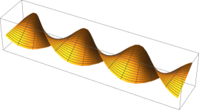
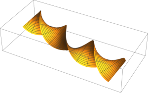
Figure 2. Minimal-energy configurations for the 1D rod model, in the case $\theta=\pi/4$. The central figure exhibits pure (constant) torsion (and zero flexure), while the other plots are characterised by (constant) $\bar{\alpha}\neq 0$ and $\bar{\beta}\neq 0$. In particular, in the rightmost picture, flexure is close to zero.

The previous analysis shows that there are many configurations realising the minimum of the 1D energy functional (2.28), at fixed $\theta$. It would be interesting to try to derive more refined and “selective” 1D models capable of breaking this degeneracy, by discriminating between the configurations shown in Fig. 2. We plan to address this issue in future work.

3. Some variants

Thin sheets of nematic elastomers with twist texture lead to a 2D model with negative target Gaussian curvature. In this section, we report on some variants of the 3D-to-2D derivation of Subsections 2.1–2.2, to explore some different scenarios. We show that nematic sheets with splay-bend texture lead to a 2D model with vanishing Gaussian target curvature (see Subsection 3.1), while nematic sheets with director uniformly aligned, and perpendicular to the mid-surface, can lead to a 2D model with positive Gaussian target curvature (see Subsection 3.2). Finally, in Subsection 3.3, we show that thin bilayer sheets provide a rich model system in which positive, zero, or negative target Gaussian curvature can be produced at will, by tuning the spontaneous strains in the two halves of the bilayer.

3.1. Splay-bend nematic elastomer sheets

In this subsection, we focus attention on a splay-bend nematic elastomer thin sheet. In this case, the distribution of the nematic director along the thickness is given by

$$\hat{n}_{h}(z_{3})\,:=\,\left(\begin{array}[]{c}\cos\big{(}\frac{\pi}{4}+\frac{\pi}{2}\frac{z_{3}}{h}\big{)}\\ 0\\ \sin\big{(}\frac{\pi}{4}+\frac{\pi}{2}\frac{z_{3}}{h}\big{)}\end{array}\right),\qquad\qquad z_{3}\in\Big{[}-\frac{h}{2},\frac{h}{2}\,\Big{]},$$

see Figure 3. Note that this distribution, which is constant on each horizontal plane, coincides with $\mathsf{e}_{1}$ on the bottom face and with $\mathsf{e}_{3}$ on the top face. Using again expression (2.7) for the energy density, the 3d-to-2d derivation is similar to that performed in Subsections 2.2–2.1. In particular, we arrive to (rescaled) spontaneous strains of the form (2.2), where now

$$B(x_{3})\,=\,\frac{1}{2}\frac{\alpha_{0}}{h_{0}}\left(\begin{array}[]{ccc}\frac{1}{3}-\cos^{2}\big{(}\frac{\pi}{4}+\frac{\pi}{2}x_{3}\big{)}&0&\frac{1}{2}\sin\big{(}\frac{\pi}{2}+\pi x_{3}\big{)}\\ 0&\frac{1}{3}&0\\ \frac{1}{2}\sin\big{(}\frac{\pi}{2}+\pi x_{3}\big{)}&0&\frac{1}{3}-\sin^{2}\big{(}\frac{\pi}{4}+\frac{\pi}{2}x_{3}\big{)}\\ \end{array}\right).$$

Recall that only the top left $2{\times}2$ part $\check{B}$ of $B$ enters into the definition of the 2D energy density $\overline{Q}_{2}$, see (2.21). Considering that the relaxed density $Q_{2}$ has the same expression as in (2.19), after some computations (see [3] for more details) we obtain, similarly to the twist case,

$$\overline{Q}_{2}(G)\,=\,\alpha_{SB}\,Q_{2}(G-\bar{A}_{SB})+\beta_{SB},\qquad\quad\mbox{for every }\ G\in\mathbb{R}^{2\times 2},$$

and in turn the limiting energy functional

$$\mathscr{F}_{lim}^{\varepsilon}(y)\,=\,\frac{1}{2}\int\limits_{\omega^{\varepsilon}}\left[\alpha_{SB}\,Q_{2}(A_{y}(x^{\prime})-\bar{A}_{SB})+\beta_{SB}\right]{\rm d}x^{\prime},\qquad\quad y\in{\rm W}^{2,2}_{\rm iso}(\omega^{\varepsilon},\mathbb{R}^{3}),$$

where

$$\alpha_{SB}\,=\,\alpha_{T}\,=\,\frac{1}{12},\quad\qquad\bar{A}_{SB}\,=\,\frac{6}{\pi^{2}}\frac{\alpha_{0}}{h_{0}}\,{\rm diag(-1,0)},\quad\qquad\beta_{SB}\,=\,\mu\,(1+\gamma)\Big{(}\frac{\pi^{4}-12}{16}\Big{)}\frac{\alpha_{0}^{2}}{h_{0}^{2}}.$$

Moreover, $\gamma$ is given in terms of the 3D parameters by (2.20). We refer the reader to [6] for the derivation of a corresponding 1D model as $\varepsilon\downarrow 0$, in the spirit of Subsection 2.3.

If $\{v_{h}\}$ a low-energy sequence of (physical) deformations, with corresponding energies $\widehat{\mathscr{F}}_{h}^{\varepsilon}(v_{h})$, we have that

$$\widehat{\mathscr{F}}_{h_{0}}^{\varepsilon}(v_{h_{0}})\,\cong\,\min_{y\in{\rm W}^{2,2}_{\rm iso}(\omega^{\varepsilon},\mathbb{R}^{3})}\frac{\mu\,h_{0}^{3}}{12}\int\limits_{\omega^{\varepsilon}}\!\!\left\{\bigg{|}{\rm A}_{y}(x^{\prime})\!-\!\frac{6}{\pi^{2}}\frac{\alpha_{0}}{h_{0}}\,{\rm diag}\big{(}-1,0\big{)}\bigg{|}^{2}\!\!+\gamma\Big{(}{\rm H}_{y}(x^{\prime})\!+\!\frac{6}{\pi^{2}}\frac{\alpha_{0}}{h_{0}}\Big{)}^{2}\!\right\}\!{\rm d}x^{\prime}\\ +\,\mu\,(1+\gamma)\,h_{0}\,\alpha_{0}^{2}\Big{(}\frac{\pi^{4}-12}{32}\Big{)}\!|\omega^{\varepsilon}|,$$

for a given small thickness $h_{0}$, where the approximate identity holds modulo terms of order higher than $3$ in $h_{0}$.

Observe that $\min\mathscr{F}_{lim}^{\varepsilon}=\beta_{SB}|\omega^{\varepsilon}|/2$, since, differently from the twist case (cf. Remark 2.2), the function $x^{\prime}\mapsto Q_{2}(A_{y}(x^{\prime})-\bar{A}_{SB})$ can be minimised to the constant value zero, by any $y\in{\rm W}^{2,2}_{\rm iso}(\omega^{\varepsilon},\mathbb{R}^{3})$ such that $A_{y}\equiv\bar{A}_{SB}$.

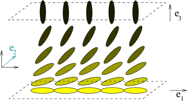
Figure 3. Sketch of the splay-bend director field.

3.2. Constant director along the thickness

In this subsection, we consider the case where the nematic director is constant along the thickness and the dependence of the spontaneous strain (2.4) on the thickness variable is encoded by the magnitude parameter $a$. More precisely, using the notation of Subsection 2.1, we suppose that the nematic director $\hat{n}(z_{3})$ is constantly equal to some $\mathsf{n}\in\mathbb{S}^{2}$, whereas the (constant) parameter $a_{h}$ in (2.5) is here replaced by the function

$$\hat{a}_{h}(z_{3})\,:=\,1+\frac{\alpha_{0}}{h_{0}}z_{3},\qquad\qquad z_{3}\in\Big{(}\!-\frac{h}{2},\frac{h}{2}\Big{)}.$$

All in all, the (physical) spontaneous strain of this system is defined as

$$\widehat{C}_{h}(z_{3})\,:=\,\hat{a}_{h}^{2/3}(z_{3})\mathsf{n}\otimes\mathsf{n}+\hat{a}_{h}^{-1/3}(z_{3})\big{(}{\rm I}-\mathsf{n}\otimes\mathsf{n}\big{)}.$$

Modelling the system using again the prototypical energy density (2.7) and following the same notation and steps of Subsections 2.1–2.2 we arrive at the rescaled energy densities $W_{h}(x_{3},\cdot)$, $x_{3}\in(-1/2,1/2)$, characterised by the (rescaled) spontaneous strains

$$\overline{C}_{h}(x_{3})\,:=\,\widehat{C}_{h}(hx_{3}) \,=\,\Big{(}1+\frac{\alpha_{0}}{h_{0}}z_{3}\Big{)}^{2/3}\!\mathsf{n}\otimes\mathsf{n}+\Big{(}1+\frac{\alpha_{0}}{h_{0}}z_{3}\Big{)}^{-1/3}\big{(}{\rm I}-\mathsf{n}\otimes\mathsf{n}\big{)}$$

$$\,=\,{\rm I}-2\,h\,B(x_{3})+R^{h}(x_{3}),\qquad\quad B(x_{3})\,:=\,\frac{x_{3}}{2}\frac{\alpha_{0}}{h_{0}}\left(\frac{\rm I}{3}-\mathsf{n}\otimes\mathsf{n}\right),$$

where $\|R^{h}\|_{\infty}=o(h)$. The corresponding 2D model that we obtain in the end associates with each $y\in{\rm W}^{2,2}_{\rm iso}(\omega^{\varepsilon},\mathbb{R}^{3})$ the energy

$$\mathscr{F}_{lim}^{\varepsilon}(y)\,=\,\frac{1}{2}\int\limits_{\omega^{\varepsilon}}\overline{Q}_{2}(A_{y}(x^{\prime})){\rm d}x^{\prime}\,=\,\frac{1}{24}\int\limits_{\omega^{\varepsilon}}Q_{2}\left(A_{y}(x^{\prime})-\check{M}\right){\rm d}x^{\prime},$$ (3.1)

where the $2{\times}2$ symmetric matrix $\check{M}$ is given by the formula

$$\check{M}\,=\,\frac{1}{2}\frac{\alpha_{0}}{h_{0}}\left[(\mathsf{n}\otimes\mathsf{n})^{\check{}}-\frac{{\rm I}_{2}}{3}\right],$$

and $(\mathsf{n}\otimes\mathsf{n})^{\check{}}$ is the $2{\times}2$ upper left part of $\mathsf{n}\otimes\mathsf{n}$. For example, in the case where $\mathsf{n}=\mathsf{e}_{3}$, we have that

$$\check{M}\,=\,\left(\begin{array}[]{ccc}m_{0}&0\\ 0&m_{0}\end{array}\right),\qquad\qquad m_{0}\,:=\,-\frac{\alpha_{0}}{6h_{0}}.$$

Notice that this corresponds to a target curvature with positive Gaussian curvature. However, observable minimal-energy configurations, will always exhibit zero Gaussian curvature, because of the isometry constraint they are subjected to. The reader is referred to [3] for more details, and for plots of minimal-energy configurations predicted by (3.1).

3.3. Bilayers

Finally, we consider the case of a bilayer governed, again, by the prototypical energy density (2.9). A similar problem has been considered in [24] and also in [8]. More precisely, we consider a model for bilayers where in the physical reference configuration $\Omega_{h}^{\varepsilon}$ the energy density $\widehat{W}_{h}=\widehat{W}_{h}(z_{3},F)$ is given by (2.8)–(2.9) and the spontaneous (right Cauchy-Green) strain is defined as

$$\widehat{C}_{h}(z_{3})\,:=\,{\rm I}\,-\,2\,h\,\widehat{B}(z_{3}),\qquad\qquad\widehat{B}(z_{3})\,:=\,\left\{\begin{array}[]{rl}M_{1}&\mbox{\ if }z_{3}\in[0,h/2)\\ M_{1}&\mbox{\ if }z_{3}\in(-h/2,0),\end{array}\right.$$

for some fixed $M_{1},M_{2}\in{\rm Sym}(3)$, whose physical dimension is that of inverse length. We again use the notation $\widehat{\mathscr{F}}_{h}^{\varepsilon}$ for the 3D (physical) free-energy functional, defined as in (2.12). Passing to the rescaled reference configuration and the corresponding rescaled energy densities $W_{h}:(-1/2,1/2)\times\mathbb{R}^{3\times 3}\longrightarrow[0,+\infty]$ defined as $W_{h}(x_{3},F):=\widehat{W}_{h}(hx_{3},F)$, we have that $W_{h}(x_{3},F)=W_{0}\big{(}F\overline{U}_{h}(x_{3})^{-1}\big{)}$, where $W_{0}$ is defined as in (2.9) and $\overline{U}_{h}(x_{3}):=\widehat{C}_{h}(hx_{3})^{1/2}$, so that

$$\overline{U}_{h}(x_{3})^{-1}\,=\,{\rm I}+h\,B(x_{3})+o(h),\qquad\mbox{with}\quad B(x_{3})\,:=\,\widehat{B}(h\,x_{3})\,=\,\left\{\begin{array}[]{rl}M_{1}&\mbox{\ if }x_{3}\in[0,1/2)\\ M_{2}&\mbox{\ if }x_{3}\in(-1/2,0).\end{array}\right.$$

The expression above shows that the spontaneous strains are compatible with the format used in [24], so that we can proceed as in Section 2 for the derivation of a limiting 2D plate model. The model is nonlinear, in the sense that it covers the regime of arbitrarily large bending deformations. The associated strains are however always small, in view of the thinness of the sheet and the fact that, in the thin limit, the mid-plane deforms isometrically. In particular, the spontaneous strains are small. Since $\overline{U}_{h}=I-hB+o(h)$, we have that the spontaneous linear (or infinitesimal) strains in the bilayer are described by

$$\widehat{E}_{h}(z_{3})\,=\,-\,h\,\widehat{B}(z_{3})\,=\,\left\{\begin{array}[]{rl}E_{1}:=\,-\,hM_{1}&\mbox{\ if }z_{3}\in[0,h/2)\\ E_{2}:=\,-\,hM_{2}&\mbox{\ if }z_{3}\in(-h/2,0),\end{array}\right.$$ (3.2)

where $E_{1}$ and $E_{2}$ are the spontaneous linear strains in the top and bottom half of the bilayer, respectively.

Proceeding as in Subsection 2.2, to which we refer for the notation, we can use again the results of [24] to deduce from the functional $h^{-2}\int_{\Omega^{\varepsilon}}W_{h}(x_{3},\nabla_{h}(y)){\rm d}x_{3}$, via compactness and $\Gamma$-convergence arguments, the 2D limit functional

$$\mathscr{F}_{lim}^{\varepsilon}(y)\,:=\,\frac{1}{2}\int\limits_{\omega^{\varepsilon}}\overline{Q}_{2}\big{(}A_{y}(x^{\prime})\big{)}{\rm d}x^{\prime},\qquad y\in{\rm W}^{2,2}_{\rm iso}(\omega^{\varepsilon},\mathbb{R}^{3}),$$ (3.3)

where

$$\overline{Q}_{2}\,:=\,\min_{D\in\mathbb{R}^{2\times 2}}\int\limits_{-1/2}^{1/2}Q_{2}\big{(}D+t\,G+\check{B}(t)\big{)}{\rm d}t,$$

and with $Q_{2}$ and $\check{B}$ defined as in (2.19)–(2.20) and (2.22), respectively. Observe that, denoting by $L$ the bilinear form associated with $Q_{2}$, namely,

$$L(G,H)\,:=\,2\mu\big{(}{\rm sym}\,G\cdot{\rm sym}\,H+\gamma\,{\rm tr}G\,{\rm tr}H\big{)},\qquad\quad G,H\in\mathbb{R}^{2\times 2},$$

we have that

$$\overline{Q}_{2}(G) \,=\,\min_{D\in\mathbb{R}^{2\times 2}}\int\limits_{-1/2}^{1/2}\Big{[}Q_{2}(D)+Q_{2}\big{(}t\,G+\check{B}(t)\big{)}+2L\big{(}D,t\,G+\check{B}(t)\big{)}\Big{]}{\rm d}t,$$

$$\,=\,\int\limits_{-1/2}^{1/2}Q_{2}\big{(}t\,G+\check{B}(t)\big{)}\,{\rm d}t+\min_{D\in\mathbb{R}^{2\times 2}}\left[Q_{2}(D)+2L\left(D,\int_{-\frac{1}{2}}^{\frac{1}{2}}\big{(}t\,G+\check{B}(t)\big{)}{\rm d}t\right)\right].$$ (3.4)

Now, simple computations give that

$$\int\limits_{-1/2}^{1/2}Q_{2}\big{(}t\,G+\check{B}(t)\big{)}\,{\rm d}t \,=\,Q_{2}(G)\int\limits_{-1/2}^{1/2}t^{2}\,{\rm d}t+\int\limits_{-1/2}^{1/2}Q_{2}\big{(}\check{B}(t)\big{)}\,{\rm d}t+2L\left(G,\int\limits_{-1/2}^{1/2}t\check{B}(t)\,{\rm d}t\right),$$

$$\,=\,\frac{1}{12}Q_{2}(G)+\frac{1}{4}L(G,\check{M}_{1}-\check{M}_{2})+\frac{1}{2}\big{[}Q_{2}(\check{M}_{1})+Q_{2}(\check{M}_{2})\big{]},$$

$$\,=\,\frac{1}{12}Q_{2}\Big{(}G+\frac{3}{2}(\check{M}_{1}-\check{M}_{2})\Big{)}+c,$$ (3.5)

where in the second equality we have used the fact that

$$\check{B}(t)\,=\,\left\{\begin{array}[]{rl}\check{M}_{1}&\mbox{\ if }t\in[0,1/2)\\ \check{M}_{2}&\mbox{\ if }t\in(-1/2,0),\end{array}\right.$$

and where we have set

$$c\,:=\,\frac{1}{16}\Big{[}5\,Q_{2}(\check{M}_{1})+5\,Q_{2}(\check{M}_{2})+6\,L(\check{M}_{1},\check{M}_{2})\Big{]}.$$

Also, note that the minimum problem in (3.4) does not depend on $G$, since $\int_{-1/2}^{1/2}t{\rm d}t=0$, so that it is equivalent to $\min_{D\in\mathbb{R}^{2\times 2}}f^{\check{B}}(D)$, where

$$f^{\check{B}}(D)\,:=\,Q_{2}(D)+2L(D,\check{N}),\qquad\qquad\check{N}\,:=\,\int\limits_{-\frac{1}{2}}^{\frac{1}{2}}\check{B}(t){\rm d}t.$$ (3.6)

It is easy to show that

$$\min_{D\in\mathbb{R}^{2\times 2}}f^{\check{B}}(D)\,=\,f^{\check{B}}(-\check{N})\,=\,-Q_{2}(\check{N})\,=\,-\frac{1}{4}Q_{2}(\check{M}_{1}+\check{M}_{1}),$$ (3.7)

where in the last equality we have used the explicit expression of $\check{B}$, and in turn that of $\check{N}$, in terms of the matrices $\check{M}_{i}$’s. Putting together (3.4), (3.5), and (3.6)–(3.7), we obtain that

$$\overline{Q}_{2}(G)\,=\,\frac{1}{12}Q_{2}\Big{(}G+\frac{3}{2}(\check{M}_{1}-\check{M}_{2})\Big{)}+c-\frac{1}{4}Q_{2}(\check{M}_{1}+\check{M}_{1})\,=\,\frac{1}{12}Q_{2}\Big{(}G+\frac{3}{2}(\check{M}_{1}-\check{M}_{2})\Big{)}-\frac{1}{16}Q_{2}(\check{M}_{1}+\check{M}_{2}).$$

All in all, turning back to the physical variables and considering a low-energy sequence of deformations $\{v_{h}\}$, we have that the limiting 2D plate theory can be summarised by the approximate identity

$$\widehat{\mathscr{F}}_{h_{0}}^{\varepsilon}(v_{h_{0}}) \,\cong\,\min_{y\in{\rm W}^{2,2}_{\rm iso}(\omega^{\varepsilon},\mathbb{R}^{3})}\frac{h_{0}^{3}}{2}\int\limits_{\omega^{\varepsilon}}\overline{Q}_{2}\big{(}{\rm A}_{y}(x^{\prime})\big{)}{\rm d}x^{\prime}$$

$$\,=\,\min_{y\in{\rm W}^{2,2}_{\rm iso}(\omega^{\varepsilon},\mathbb{R}^{3})}\frac{h_{0}^{3}}{24}\int\limits_{\omega^{\varepsilon}}Q_{2}\Big{(}{\rm A}_{y}(x^{\prime})-\frac{3}{2h_{0}}(\check{E}_{1}-\check{E}_{2})\Big{)}{\rm d}x^{\prime}-\frac{h_{0}|\omega^{\varepsilon}|}{32}Q_{2}(\check{E}_{1}+\check{E}_{2}),$$

where $Q_{2}$ is defined as in (2.19)–(2.20), and $\check{E}_{1}$ and $\check{E}_{2}$ denote the sub-matrices consisting of the first two rows and columns of the spontaneous linear strains in the top and bottom part of the bilayer, respectively, see (3.2). Depending on the values the components of $\check{E}_{1}$ and $\check{E}_{2}$, one can obtain target curvature tensors $3(\check{E}_{1}-\check{E}_{2})/2h_{0}$ with positive, zero, or negative determinant, and hence positive, zero, or negative target Gaussian curvature. In all cases, however, the isometry constraint will have the effect that energy minimising configurations will be ribbons wrapped around a cylinder.

4. Conclusions and discussion

In this paper, we have discussed a strategy to derive a model for nematic elastomer thin and narrow films, with a twist nematic texture. The strategy uses a rigorous dimension reduction argument, from 3D to 2D (plate model), and then from 2D to 1D (narrow ribbon model). This procedure leads to a degenerate model, which admits as minimisers both spiral ribbons and helicoid-like shapes. It would be interesting to derive more selective 1D models, able to discriminate between these two types of configurations, and to deliver unique minimisers in different regimes of the relevant material and geometric parameters governing the behaviour of thin and narrow strips. This will be attempted in future work. We refer the reader to [26] for further discussion of spiral ribbon vs. helicoid-like shapes in thin sheets of nematic elastomers.

In addition, we have considered variants to thin nematic sheets with twist texture, which leads to 2D models with negative Gaussian target curvature. In the context of nematic elastomers, these are the splay-bend texture and uniform alignment of the director perpendicular to the mid-plane, which lead to zero and positive Gaussian target curvature, respectively. We have also shown that thin bilayer sheets provide a rich model system in which positive, zero, or negative target Gaussian curvature can be produced at will, by tuning the spontaneous strains in the two halves of the bilayer.

Acknowledgements

We thank E. Sharon for valuable discussions. We gratefully acknowledge the support by the European Research Council through the ERC Advanced Grant 340685-MicroMotility.

The authors declare that they have no conflict of interest.

References

• [1] V. Agostiniani, T. Blass, and K. Koumatos. From nonlinear to linearized elasticity via $\Gamma$ -convergence: the case of multiwell energies satisfying weak coercivity conditions. Math. Models Methods in Appl. Sci., 25(01):1–38, 2015.
• [2] V. Agostiniani, G. Dal Maso, and A. DeSimone. Attainment results for nematic elastomers. Proc. Roy. Soc. Edinburgh Sect. A, 145:669–701, 8 2015.
• [3] V. Agostiniani and A. DeSimone. Rigorous derivation of active plate models for thin sheets of nematic elastomers. http://arxiv.org/abs/1509.07003, submitted for publication.
• [4] V. Agostiniani and A. DeSimone. $\Gamma$-convergence of energies for nematic elastomers in the small strain limit. Contin. Mech. Thermodyn., 23(3):257–274, 2011.
• [5] V. Agostiniani and A. DeSimone. Ogden-type energies for nematic elastomers. Internat. J. Non-Linear Mech., 47(2):402–412, 2012.
• [6] V. Agostiniani, A. DeSimone, and K. Koumatos. Shape programming for narrow ribbons of nematic elastomers. Journal of Elasticity, pages 1–24, 2016.
• [7] H. Aharoni, E. Sharon, and R. Kupferman. Geometry of thin nematic elastomer sheets. Phys. Rev. Lett., 113:257801, Dec 2014.
• [8] S. Bartels, A. Bonito, and R. H. Nochetto. Bilayer plates: model reduction, $\Gamma$-convergent finite element approximation and discrete gradient flow. http://arxiv.org/abs/1506.03335.
• [9] K. Bhattacharya, A. DeSimone, K. F. Hane, R. D. James, and C. J. Palmstrøm. Tents and tunnels on martensitic films. Materials Science and Engineering: A, 273–275:685–689, 1999.
• [10] P. Bladon, E. M. Terentjev, and M. Warner. Transitions and instabilities in liquid crystal elastomers. Phys. Rev. E, 47:R3838–R3840, Jun 1993.
• [11] P.G. Ciarlet. An Introduction to Differential Geometry with Applications to Elasticity. Available online. Springer, 2006.
• [12] S. Conti, A. DeSimone, and G. Dolzmann. Semisoft elasticity and director reorientation in stretched sheets of nematic elastomers. Phys. Rev. E, 66:061710, Dec 2002.
• [13] S. Conti, A. DeSimone, and G. Dolzmann. Soft elastic response of stretched sheets of nematic elastomers: a numerical study. J. Mech. Phys. Solids, 50(7):1431 – 1451, 2002.
• [14] A. DeSimone. Energetics of fine domain structures. Ferroelectrics, 222:275–284, 1999.
• [15] A. DeSimone and G. Dolzmann. Macroscopic response of nematic elastomers via relaxation of a class of $\rm SO(3)$-invariant energies. Arch. Ration. Mech. Anal., 161(3):181–204, 2002.
• [16] P.J. Flory. Principles of Polymer Chemistry. Baker lectures 1948. Cornell University Press, 1953.
• [17] L. Freddi, P. Hornung, M. G. Mora, and R. Paroni. A corrected Sadowsky functional for inextensible elastic ribbons. J. Elasticity, pages 1–12, 2015.
• [18] G. Friesecke, R. D. James, and S. Müller. A theorem on geometric rigidity and the derivation of nonlinear plate theory from three-dimensional elasticity. Comm. Pure Appl. Math., 55(11):1461–1506, 2002.
• [19] A. Lucantonio, G. Tomassetti, and A. DeSimone. Large-strain poroelastic plate theory for polymer gels with applications to swelling-induced morphing of composite plates. Composites Part B: Engineering, pages –, 2016.
• [20] P. Nardinocchi, E. Puntel. Unexpected hardening effects in bilayered gel beams. To appear on Meccanica, doi: 10.1007/s11012-017-0635-z.
• [21] P. Petersen. Riemannian geometry, volume 171 of Graduate Texts in Mathematics. Springer, New York, second edition, 2006.
• [22] Y. Sawa, K. Urayama, T. Takigawa, A. DeSimone, and L. Teresi. Thermally driven giant bending of liquid crystal elastomer films with hybrid alignment. Macromolecules, 43:4362–4369, May 2010.
• [23] Y. Sawa, F. Ye, K. Urayama, T. Takigawa, V. Gimenez-Pinto, R. L. B. Selinger, and J. V. Selinger. Shape selection of twist-nematic-elastomer ribbons. PNAS, 108(16):6364–6368, 2011.
• [24] B. Schmidt. Plate theory for stressed heterogeneous multilayers of finite bending energy. J. Math. Pures Appl., 88(1):107 – 122, 2007.
• [25] L. Teresi and V. Varano. Modeling helicoid to spiral-ribbon transitions of twist-nematic elastomers. Soft Matter, 9:3081–3088, 2013.
• [26] G. Tomassetti, V. Varano. Modeling of distortion-induced spiral to ribbon transitions. To appear on Meccanica, doi: 10.1007/s11012-017-0631-3.
• [27] K. Urayama. Switching shapes of nematic elastomers with various director configurations. Reactive and Functional Polymers, 73(7):885–890, 2013. Challenges and Emerging Technologies in the Polymer Gels.
• [28] M. Warner and E. M. Terentjev. Liquid crystal elastomers. Clarendon Press, Oxford, 2003.