The Molecular Structures of the Local Arm and Perseus Arm
in the Galactic Region of l = [139^∘.75, 149^∘.75] , b = [$-$5^∘.25, 5^∘.25]

Abstract

Using the Purple Mountain Observatory Delingha (PMODLH) 13.7 m telescope, we report a 96-square-degree ¹²CO/¹³CO/C¹⁸O mapping observation toward the Galactic region of $l=[139.75,149.75]^{\circ}$, $b=[-5.25,5.25]^{\circ}$. The molecular structures of Local Arm and Perseus Arm are presented. Combining H I data and part of the Outer Arm results, we obtain that the warp structure of both atom and molecular gas is obvious, while the flare structure only exists in atomic gas in this observing region. In addition, five filamentary giant molecular clouds on the Perseus Arm are identified. Among them, four are newly identified. Their relations with Milky Way large scale structure are discussed.

1 Introduction

The Milky Way (MW) galaxy is our home galaxy. Since we are located at the Galactic plane, which is full of gas and dust, the difficulty in studying its structure is greater than that for some external galaxies. Up to now, although many previous works have already revealed its global appearance (e.g., Bok 1959; Oort et al. 1958; Georgelin & Georgelin 1976), its detailed structure is still under debate (e.g., Russeil et al. 2007; Vallée 2008; Reid et al. 2014). For researching the Milk Way structure, the most basic requirement is the high-quality and large-scale survey data. In the past several decades, lots of molecular line surveys, especially the CO line surveys have been conducted (cf. Heyer & Dame 2015). Among them, two most remarkable CO surveys conducted by Heyer et al. (1998) and Dame et al. (2001) have provided a lot of precious data. Currently, many MW models are largely based on those two surveys (e.g., Hou & Han 2014). However, such data with relatively low resolution or low sensitivity gradually become insufficient for more detailed research. Fortunately, the on-going Milky Way Imaging Scroll Painting (MWISP) project , which is the first no-bias, high sensitive large-scale ¹²CO/¹³CO/C¹⁸O survey toward the Galactic plane, somewhat solves such problem. As one of the target regions of the survey, a Galactic region of $l=[139.75,149.75]^{\circ}$, $b=[-5.25,5.25]^{\circ}$ (hereafter the G140 Region) has been completely covered by nearly 2 yr of observation. The total observing area is 105-square-degree, and this paper takes a 96-square-degree part (cf. Figure 2 for the used part) to study the spiral arm structure. Another 9-square-degree part has been used for another study which will be published soon (Xiong et al. 2017, to be accepted).

The G140 Region is located in the second quadrant of the MW, which is a better place to study the arm structure since the kinematic distance here is the monotonic function of LSR velocity. Starting from $V_{\mathrm{LSR}}\sim 0$ km s^-1, increasingly negative velocities successively trace the Local Arm, the Perseus Arm, the Outer Arm and a new segment of spiral arm discovered by Sun et al. (2015) (hereafter New Arm). In most MW spiral arm models, the Perseus Arm, the Outer Arm, and the New Arm all comprise the major spiral arm of the MW (cf. Steiman-Cameron 2010; Sun et al. 2015). The Local Arm was once thought to be a spur structure, until recently, when Xu et al. (2013, 2016) provided strong observational evidences to prove that it is a larger structure, such as a branch.

Interestingly, since the G140 Region is just the intersection point of the Gould Belt and the Galactic plane (cf. Figure 2 in Grenier 2004), the Local Arm in this place is made up of two layers — the Gould Belt layer which is associated with the Lindblad Ring traced by H I gas (Lindblad 1967; Strauss et al. 1979), and the Cam OB1 layer which is associated with the Cam OB1 association (Digel et al. 1996; Straižys & Laugalys 2008). The Cam OB1 layer is a star-forming active layer that locates the famous young stellar object GL 490 and two Sharpless H II regions, as well as the Cam OB1 association. The star-forming activities in this region have been studied in detail by Straižys & Laugalys (2007) and their series of works. But the molecular cloud structure of this region was rarely studied. Except for a small part studied by Digel et al. (1996), up to now there has been no systematic CO observation completely covered this region.

In this paper, we report the ¹²CO/¹³CO/C¹⁸O mapping observation toward the G140 Region. We mainly focus on studying the molecular structure of Local Arm and Perseus Arm here. The study of star forming-activity will be presented in our next paper. Section 2 presents the CO observation condition and archival data of atomic hydrogen. Section 3 presents the physical parameters of Local Arm and Perseus Arm derived by CO data. Combing H I data and part of Outer Arm results (Du et al., 2016), Section 4 discusses the arm structures in the G140 Region. Section 5 presents five filamentary giant molecular clouds identified in the Perseus Arm and discusses their relations to the MW large-scale structure. Finally, Section 6 presents the summary.

2 Observation

2.1 CO Observation

The ¹²CO ($1-0$), ¹³CO ($1-0$) and C¹⁸O ($1-0$) lines were observed using the Purple Mountain Observatory Delingha (PMODLH) 13.7 m telescope from 2013 September to 2015 December as one of the scientific demonstration regions for the MWISP project. The three lines were observed simultaneously with the nine-beam superconducting array receiver (SSAR) working in sideband separation mode and with the fast Fourier transform spectrometer (FFTS) employed (Shan et al., 2012). The ¹²CO line is at the upper sideband (USB), and the ¹³CO and C¹⁸O lines are at the lower sideband (LSB). Both of the bandwidths are 1000 MHz with 16,384 channels. With on-the-fly (OTF) observing mode, an area of $l=[139.75,149.75]^{\circ}$, $b=[-5.25,5.25]^{\circ}$ (105-square-degree in total) was covered, and a 96-square-degree part is used in this work. All the data were sampled every $30^{\prime\prime}$. For the ¹²CO observations (@ USB), the main beam width was about $49^{\prime\prime}$, the main-beam efficiency ($\eta_{\mathrm{MB,USB}}$) was about 0.46, and the typical rms noise level was about 0.5 K corresponding to a channel width of 0.16 km s^-1; For the ¹³CO and C¹⁸O observations (@ LSB), the main beam width was about $51^{\prime\prime}$, the main-beam efficiency ($\eta_{\mathrm{MB,LSB}}$) was about 0.48, and the typical rms noise level was about 0.3 K corresponding to a channel width of 0.17 km s^-1. All the data were corrected by $T_{\mathrm{MB}}=T^{*}_{\mathrm{A}}/\eta_{\mathrm{MB}}$.

2.2 Archival Data of Atomic Hydrogen

The 21 cm line data were retrieved from the Canadian Galactic Plane Survey (CGPS; Taylor et al. 2003). We downloaded data of $l=[140,150]^{\circ}$, $b=[-3,5]^{\circ}$ from the Canadian Astronomy Data Centre. The velocity coverage of the data is in the range of -153 to 40 km s^-1 with a channel separation of 0.82 km s^-1. The survey has a spatial resolution of $58^{\prime\prime}$, which is comparable to our CO observations.

3 Physical Parameters

3.1 Slicing the Region

Figure 1 presents the LSR velocity distribution of the G140 Region. The ¹²CO, ¹³CO and C¹⁸O FITS cube data of the whole region were integrated over all latitudes with 3$\sigma$ thresholds (namely, ¹²CO emission $\lesssim$ 1.5 K and ¹³CO/C¹⁸O emission $\lesssim$ 0.9 K are not integrated). Then three high signal-to-noise ratio $l-V$ maps of those molecules are obtained. Since the velocity resolutions are not the same (0.16 km s^-1@ ¹²CO and 0.17 km s^-1@ ¹³CO/C¹⁸O), the velocity dimensions of the ¹³CO and C¹⁸O $l-V$ maps have been interpolated for comparison with the ¹²CO data. Then, we define Mask 1 as the area where only ¹²CO emission exists, Mask 2 as the area where ¹²CO and ¹³CO emission both exist but C¹⁸O emission does not, and Mask 3 as the area where ¹²CO, ¹³CO and C¹⁸O emission all exists. The blue, green, and red colors in Figure 1 indicate Mask 1, Mask 2, and Mask 3, respectively. Obviously, from LSR velocity $\sim$ 10 to $-50$ km s^-1 the Gould Belt layer, Cam OB1 layer, and Perseus arm are successively located. The black lines in Figure 1 outline their boundaries. In addition, some Outer Arm and New Arm structure can also be seen in this map because of the high-quality data. In order to show those two arms more clearly, the molecular clouds and arm spiral projections (identified and fitted by Sun et al. 2015 and Du et al. 2016, see the caption of Figure 1 for more details) are plotted.

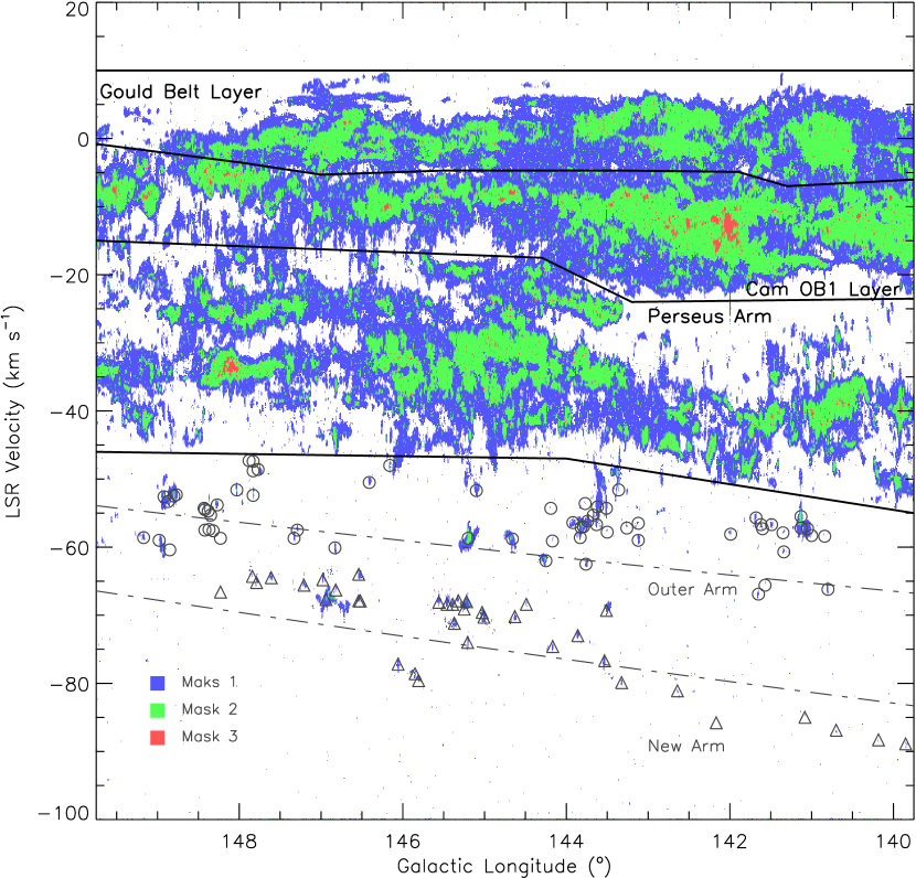
Figure 1: Longitude-velocity map of the whole area. The blue, green, and red colors indicate Mask 1, Mask 2, and Mask 3, respectively. (The meanings of the masks are presented in Section 3.1.) The Gould Belt layer, Cam OB1 layer, and Perseus Arm are divided by solid lines. The circles and triangles present the Outer Arm clouds (identified by Du et al. 2016) and the New Arm clouds (identified by Sun et al. 2015 and Du et al. 2016). The two dashed lines indicate the projections of the Outer Arm spiral (fitted by Du et al. 2016) and the New Arm spiral (fitted by Sun et al. 2015), respectively.

According to the $l-V$ map, the FITS cube of the three molecules is integrated over the velocity ranges, which are shown as the black lines in Figure 1. Also the integrated thresholds are 3$\sigma$. Then the integrated intensity maps of the three molecules are obtained. We also define Mask 1, Mask 2, and Mask 3 of the integrated maps, and the definitions of the masks are the same as in the above presentation. Figure 2 shows the final results. It can be seen that lots of molecular gas presents filamentary structure, especially in the Perseus Arm (this will be discussed in Section 5). In addition, C¹⁸O is not rich in this region: it is rarely distributed on the Gould Belt layer, some is concentrated on the position of $(l,b)\sim(140,2)$^∘ (where locates the GL 490) on the Cam OB1 layer, and on the Perseus Arm some is distributed on the position of $(l,b)\sim(148,0)$^∘. This roughly indicates that the gas is relatively less dense in this region.

The distance of the Local Arm in this region has many photometric results. The distance of the Gould Belt layer is in the range of 160 – 300 pc (Straižys et al. 2001; Zdanavičius et al. 2005), and the Cam OB1 layer is about 1.0 kpc far away from us (Humphreys 1978; Lyder 2001; Straižys & Laugalys 2007). Although there is no photometric distance of the Perseus Arm in this region, the nearby high-mass star-forming regions W 3OH (i.e. G133.94+01.06) and S Per (i.e. G134.62-02.19) have the trigonometric parallax results, which are 1.95 kpc (Xu et al., 2006) and 2.42 kpc (Asaki et al., 2010), respectively. In addition, according to the Perseus Arm spiral fitted by Reid et al. (2014), at the positions of $(l,b)=(140,0)$^∘ and $(l,b)=(150,0)$^∘, the distances are calculated to be 2.0 and 2.2 kpc, respectively. Based on all the distance results presented above, we finally adopt 200 pc, 1.0 kpc, and 2.1 kpc as the distances of the Gould Belt layer, Cam OB1 layer, and Perseus arm, respectively.

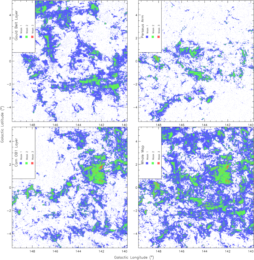
Figure 2: Mask maps of the Gould Belt layer (top left panel), the Cam OB1 layer (bottom left panel), the Perseus Arm (top right panel) and the whole area (bottom right panel). The blue, green, and red color indicate Mask 1, Mask 2, and Mask 3, respectively. (The meanings of the masks are presented in Section 3.1.) Note that the data in the upper left corner of each panel (where the insert is located) were not used in this paper, since they have been used for another study that will be published soon (Xiong et al. 2017, to be accepted).

3.2 Physics of Layers

Assuming that ¹²CO is optically thick, following Bourke et al. (1997), the excitation temperature ($T_{\mathrm{ex}}$) in each pixel of each layer can be calculated by

$$T_{\mathrm{ex}}=\frac{h\nu_{12}/k}{\ln(1+\frac{h\nu_{12}/k}{T_{\mathrm{MB,^{12}CO}}+\frac{h\nu_{12}/k}{\exp(h\nu_{12}/T_{\mathrm{bg}}-1)}})}$$ (1)

where $h$ is the Planck constant, $k$ is the Boltzmann constant, $\nu_{12}$ is the frequency of ¹²CO, $T_{\mathrm{MB,^{12}CO}}$ is the peak main-beam temperature in each pixel, and $T_{\mathrm{bg}}$ is the temperature of the cosmic microwave background. The equation can be simplified as

$$T_{\mathrm{ex}}=\frac{5.532}{\ln(1+\frac{5.532}{T_{\mathrm{MB,^{12}CO}}+0.819})}\quad\mathrm{K}$$ (2)

when all the constants are substituted.

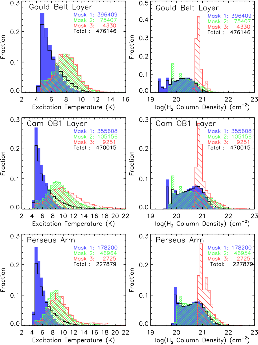
Figure 3: Distributions of $T_{\mathrm{ex}}$ and H₂ column density of each layer. The blue, green, red, and black colors in each panel indicate the distributions of Mask 1, Mask 2, Mask 3, and the three masks in total, respectively. The numbers with corresponding colors in each panel represent the pixel numbers.

The three left panels of Figure 3 show the distributions of $T_{\mathrm{ex}}$ in the three layers. It can be seen that the excitation temperatures in this region are relatively low. In the Cam OB1 layer, most of the $T_{\mathrm{ex}}$ of Mask 3 are in the range of 6 – 16 K, which are slightly higher than the other two layers ($T_{\mathrm{ex}}$ $\sim$ 6 – 12 K). The reason may be that the Cam OB1 layer has more star-forming activities. Moreover, in each layer the $T_{\mathrm{ex}}$ peak distributions of Mask 1, Mask 2, and Mask 3 are in the increasing trend. This may indicate that the region where C¹⁸O exists is relatively hotter and the region where only ¹²CO exists is relatively colder.

The H₂ column densities of the three masks are calculated by two different methods. For Mask 1, where only ¹²CO is detected, we use the X-factor to estimate the column density (hereafter the X-factor method):

$$N_{\mathrm{Mask1,H_{2}}}=X\int T_{\mathrm{MB,^{12}CO}}dV$$ (3)

where $\int T_{\mathrm{MB,^{12}CO}}dV$ is the integrated intensity of ¹²CO in each pixel, and the factor X is adopted from the results of Abdo et al. (2010), namely, $0.87\times 10^{20}$ cm^-2 (K $\cdot$ km s^-1)^-1 in the Gould Belt layer, $1.59\times 10^{20}$ cm^-2 (K $\cdot$ km s^-1)^-1 in the Cam OB1 layer, and $1.9\times 10^{20}$ cm^-2 (K $\cdot$ km s^-1)^-1 in the Perseus Arm.

For Mask 2 and Mask 3, the local thermodynamic equilibrium (LTE) condition is assumed. Then, assuming that ¹³CO and C¹⁸O are optically thin and they share the same $T_{\mathrm{ex}}$ with ¹²CO, following Bourke et al. (1997) and Pineda et al. (2010), the ¹³CO column density of Mask 2 in each pixel can be calculated by

$$N_{\mathrm{Mask2,^{13}CO}}=2.42\times 10^{14}\frac{\tau_{13}}{1-e^{-\tau_{13}}}\frac{\int T_{\mathrm{MB,^{13}CO}}dV}{1-e^{-5.29/T_{\mathrm{ex}}}}\quad\mathrm{cm^{-2}}$$ (4)

and for Mask 3 the C¹⁸O column density in each pixel can be calculated by

$$N_{\mathrm{Mask3,C^{18}O}}=2.42\times 10^{14}\frac{\tau_{18}}{1-e^{-\tau_{18}}}\frac{\int T_{\mathrm{MB,C^{18}O}}dV}{1-e^{-5.27/T_{\mathrm{ex}}}}\quad\mathrm{cm^{-2}}$$ (5)

where $\tau_{13}$ and $\tau_{18}$ respectively indicate the peak optical depth of ¹³CO and C¹⁸O, $\int T_{\mathrm{MB,^{13}CO}}dV$ and $\int T_{\mathrm{MB,C^{18}O}}dV$ respectively indicate the integrated intensities of ¹³CO and C¹⁸O in units of K $\cdot$ km s^-1, and $T_{\mathrm{ex}}$ is in units of K. And $\tau_{13}$ and $\tau_{18}$ are calculated by

$$\tau_{13}=-\ln[1-\frac{T_{\mathrm{MB,^{13}CO}}}{5.29}([e^{5.29/T_{\mathrm{ex}}}-1]^{-1}-0.16)^{-1}]$$ (6)

and

$$\tau_{18}=-\ln[1-\frac{T_{\mathrm{MB,C^{18}O}}}{5.27}([e^{5.27/T_{\mathrm{ex}}}-1]^{-1}-0.17)^{-1}]$$ (7)

Where $T_{\mathrm{MB,^{13}CO}}$ and $T_{\mathrm{MB,C^{18}O}}$ are the peak main-beam temperatures of ¹³CO and C¹⁸O, respectively. Finally, according to the abundances of ¹³CO and C¹⁸O (Ferking et al. 1982; Castets & Langer 1995), the H₂ column density of Mask 2 and Mask 3 in each pixel can be calculated by

$$N_{\mathrm{Mask2,H_{2}}}=7\times 10^{5}\times N_{\mathrm{Mask2,^{13}CO}}$$ (8)

and

$$N_{\mathrm{Mask3,H_{2}}}=7\times 10^{6}\times N_{\mathrm{Mask3,C^{18}O}}$$ (9)

Hereafter this column density estimation method is called the LTE method for short in this paper.

Table 1: Layer Parameter

Layer	Mask	Pixel	Pixel	Area	Mass
Name	Name	Number	Percentage	(pc2)	(M⊙)
Gould Belt	Mask 1	396,409	83.3%	335	1,607
	Mask 2	75,407	15.8%	64	503
	Mask 3	4,330	0.9%	4	63
	Total	476,146		400	2,200
Cam OB1	Mask 1	355,608	75.6%	7,522	77,395
	Mask 2	105,156	22.4%	2,224	42,464
	Mask 3	9,251	2.0%	196	7,394
	Total	470,015		9,900	127,300
Perseus Arm	Mask 1	178,200	78.2%	16,624	198,130
	Mask 2	46,954	20.6%	4,380	82,472
	Mask 3	2,725	1.2%	254	8,787
	Total	227,879		21,300	289,400

Figure 4 shows the H₂ column density result of the whole region. Clearly, the $N_{\mathrm{H_{2}}}$ in the main part of the gas is about $10^{21}$ to $10^{21.5}$ cm^-2. The three right panels of Figure 3 show the H₂ column density distribution of the three layers. One can see that the $N_{\mathrm{H_{2}}}$ distribution of Mask 3 is much more concentrated (around a higher value of $10^{21}$ cm^-2) than that of Mask 2 and Mask 3. This indicates that the region traced by C¹⁸O is relatively denser.

Knowing the $N_{\mathrm{H_{2}}}$ in each pixel, we can then estimate the mass of each mask:

$$M_{\mathrm{Mask}}=2\mu m_{\mathrm{H}}a^{2}d^{2}\Sigma N_{\mathrm{Mask,H_{2}}}$$ (10)

where $\mu$ (=1.36, Hildebrand 1983) is the mean atomic weight per H atom in the ISM, $m_{\mathrm{H}}$ is the H atom mass, $a$ (=30^′′) is the angular size of each pixel, $d$ is the distance of each layer (see Section 3.1), and $\Sigma N_{\mathrm{Mask,H_{2}}}$ refers to the $N_{\mathrm{H_{2}}}$ summation of all the pixels in each mask. Table 1 shows the final results of pixel number, pixel percentage (the ratio of pixel number in one mask to the total pixel number in three masks), physical area (the physical area is estimated by “one pixel physical area” $\times$ “pixel number”), and mass of each mask in each layer. It is noticeable that the pixel percentage of Mask 2 and Mask 3 the in Cam OB1 layer is higher than that of other two layers. This is perhaps because the Cam OB1 layer have more star-forming activities.

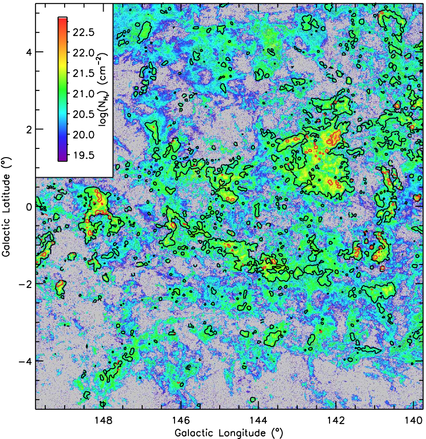
Figure 4: H₂ column density of the whole area. The black and red lines confine Mask 2 and Mask 3, respectively. The rest of the area is Mask 1.

4 Arm Structure

4.1 Gas Distribution

Most works about the gas distribution of the MW are mainly focused on the global and radial structure (e.g., Burton et al. 1975; Sodroski et al. 1987; Nakanishi & Sofue 2003 and their serial papers; Duarte-Cabral et al. 2015). The distribution along the arm spiral direction is also meaningful. For example, in the study of external galaxies by La Vigne et al. (2006), the feather structure is well associated with the gas peak surface density (see Figure 19 – 20 of their paper). Their work presented a good way of thinking about studying the substructure of our MW. Substructures such as the branch, spur, and feather will be discussed in detail in Section 5. In this section we just focus on the gas distribution along the Galactic longitude.

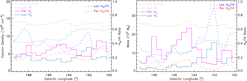
Figure 5: Column density (left panel) and mass (right panel) distributions of H₂ and H I gases along the Galactic longitude. Note that the column density and mass of H I gas are divided by 2 and 5, respectively.

Figure 5 shows the distributions of H I and H₂ gases of the Local Arm and Perseus Arm along the Galactic longitude. Since the Local Arm shares two layers, the $N_{\mathrm{H_{2}}}$ in each pixel of this arm is obtained by calculating the mean value in the same angular position of the Gould Belt layer and the Cam OB1 layer, while the H₂ mass is obtained by adding together the data of the two layers. Then, we calculate the mean value of $N_{\mathrm{H_{2}}}$ every 0.2 Galactic longitude degree of the Local Arm and the Perseus Arm, respectively. Thus the $N_{\mathrm{H_{2}}}$ distribution is obtained. And for the H₂ mass distribution, we calculate the summation of H₂ mass every 0.2 Galactic longitude degree. To obtain the parameters of H I gas, we first slice the data into three layers just as the same LSR velocity ranges of Section 3.1. Second, assuming that H I is optically thin, the surface density of each layer is calculated by $\Sigma_{\mathrm{HI}}=1.82\times 10^{18}m_{\mathrm{H}}\int T_{\mathrm{MB,HI}}d\,V$, where $\int T_{\mathrm{MB,HI}}d\,V$ is the integrated intensity of H I. And then the H I column density is obtained by the relation of $\mathrm{1\ M_{\odot}pc^{-2}=1.25\times 10^{20}\ \ cm^{-2}}$. Third, combining the distance, the mass of H I in each pixel can be easily obtained, and the calculation method is the same as the one in Section 3.2. Finally, the H I column density and mass distributions along the Galactic longitude are obtained just using the same approaches of H₂ that have been presented above, and the column density and mass ratios of H₂ and H I gas are simply calculated by division.

Table 2: Gas Mass of Spiral Arm

Spiral	H2	H I	H2 + H I	H2 / H I
Arm	(104M⊙)	(104M⊙)	(104M⊙)
Local	9	25	34	0.36
Perseus	21	247	268	0.08
Outer	15	624	639	0.02

In Figure 5 one can see that the gases in both the two arms vary smoothly, especially the H I gas. In addition, the H₂ column densities of the Local Arm and Perseus Arm are similar, and the H₂ mass of the Perseus Arm is a little higher than that of the Local Arm. However, the H I gas exhibits a largely different performance. Both the column density and mass of H I gas on the Perseus Arm are much higher than those on the Local Arm. Thus, the ratio of H₂ to H I (hereafter the H₂/H I) of the Local Arm is higher than that of the Perseus Arm. This condition is also clearly shown in Table 2, which summarizes the gas masses of the Local Arm and Perseus Arm and also lists the masses of Outer arm in G140 Region for comparison (the Outer Arm data are obtained from Du et al. 2016). Since both the Outer Arm and Perseus Arm are the major spiral arm of MW and the Outer Arm is located farther away from the Galactic center (see Section 1), it may be reasonable that H₂/H I of the former is lower than that of the latter. However, that the Local Arm — as a subarm of the MW — has the highest H₂/H I is somewhat abnormal. Maybe it indicates a tendency that the H₂ gas is more compactly located around the Galactic center than that of H I gas. However, another probable reason should NOT be ignored — that the H I gas on the Local Arm is largely underestimated. This will be presented in Section 4.2

4.2 Warp and Flare

Warp is a common phenomenon among disk galaxies (Binney, 1992). The external galaxies with optical warps have long been recognized (Sandage 1961; Arp 1966), but they were just thought to be some special cases since only a few were observed at that time. Using H I gas observation data, Sancisi (1976) found that four out of five galaxies were gaseous warped. Thereafter more gas warps were identified in a large number of external galaxies (e.g., Huchtmeier et al. 1980; García-Ruiz et al. 2002). As it deserved, from that time on warp was regarded with special attention. With no exception, our MW is also a warped galaxy. In fact, the H I gas warp was observed very early on (Burke 1957; Kerr 1957; Kerr et al. 1957; westerhout 1957). The warp of our Galaxy has a large amplitude and is also asymmetric (Levine et al., 2006). Combing recent H I observation data, Kalberla & Kerp (2009) summarized a bended Galactic plane map (Figure 3 in their paper), which showed a general distribution of Galactic warp. Besides H I gas, the MW warp has been observed and studied by many other tracers, such as dust (Freudenreich et al., 1994), CO (Wouterloot et al., 1990), stars or OB stars (Miyamoto et al. 1988; Dehnen 1998), and IRAS point sources (Djorgovski & Sosin, 1989). Besides warp, flare — as another gas behavior— is also an interesting phenomenon among galaxies, as well as our Galaxy. In addition, the MW flare has been confirmed in both gaseous and stellar tracers (e.g., Momany et al. 2006; Kalberla & Kerp 2009; Heyer & Dame 2015). Usually flare and warp are discussed together under the hypothesis that they are the response of dark matter (e.g., Binney 1978; Kalberla et al. 2007). Unlike the difficult research situation in the MW spiral structure, the study of warp and flare in the MW is relatively less troublesome since the inclination problem that always exists among external galaxies can be discarded. In this exact G140 Region, we will morphologically present the warp and flare of both H I and H₂ gases in the following paragraphs.

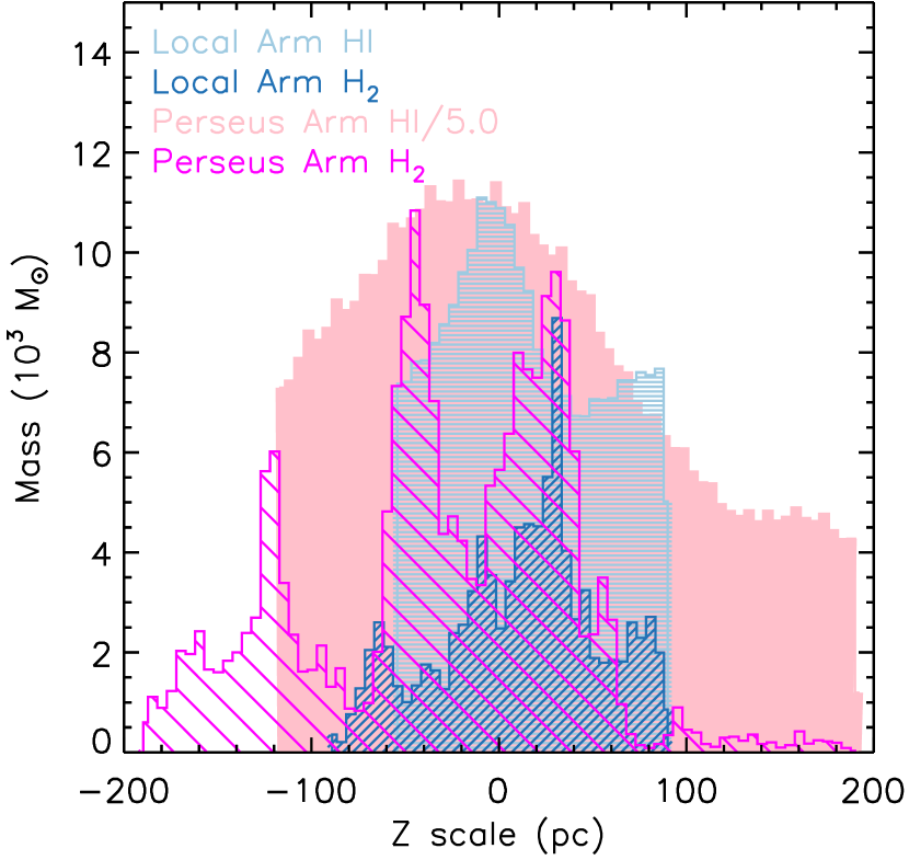
Figure 6: Gas distribution of the Local Arm and Perseus Arm along the Z scale. Note that the mass of H I gas of the Perseus Arm is divided by 5.

Figure 6 shows the mass distributions of H₂ and H I gas on the Local Arm and Perseus Arm along the Z scale. First, according to the Galactic latitude and distance, we calculate the Z scale of every pixel of each layer. Second, we calculate the total mass of every 5 pc Z scale of each layer; thus, we can get the gas distributions of 3 layers. Then, we add the distributions of the Gould Belt layer and Cam OB1 layer as the Local Arm gas distribution, and the distributions of the two spiral arms are finally obtained. Obviously, the gas distribution is incomplete, due to the limited observation scope along the Galactic latitude. Some H₂ gas on the Local Arm seems to be not completely observed — the H₂ gas mass suddenly becomes zero at a Z scale of about 90 pc (where $b\sim 5$^∘). In addition, part of the H I gas on the Perseus Arm and large amount of H I gas on Local Arm are not completely observed. The distributions suddenly stop at Z scales of about -120, -60, 90, and 200 pc, respectively. In other words, the total mass of H I gas on the two spiral arms, especially on the Local Arm, is largely underestimated (which is one of the probable reason that the H₂/HI of the Local Arm is largely higher than that of the Perseus Arm mentioned in Section 4.1).

Table 3: Thickness and Height of Arm

Spiral	Thickness		Height
Arm	H2	H I	H2	H I
	(pc)	(pc)	(pc)	(pc)
Local	117	220	18	-2
Perseus	149	291	-16	-19
Outer	60	550	170	160

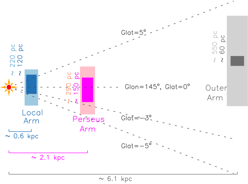
Figure 7: Sketch map of the thicknesses and heights of three spiral arms. The Galactic latitudes plotted are proportionally zoomed in. The light-blue, pink, and light-gray rectangles indicate the H I gas of the Local Arm, Perseus Arm, and Outer Arm, respectively. The dark-blue, magenta, and dark gray-rectangles indicate the H₂ gas of the three arms. The numbers with corresponding colors beside the rectangles mark the thickness values of H I and H₂ gases of the arms.

Despite the incomplete Z scale gas distribution, we can still estimate the thickness and height of each arm by fitting the distribution in a Gaussian curve. We define the FWHM as the arm thickness and the centric position at Z scale as the arm height. Table 3 lists the final results, as well as the parameters of the Outer Arm in the G140 Region for comparison (data from Du et al. 2016). A more direct perspective on the arm distributions can be seen in Figure 7. We obtain the mean distance of the Gould Belt layer and Cam OB1 layer as the distance of the Local Arm. For the Outer Arm distance, we adopt the mean distance of all the Outer Arm clouds in the G140 Region with the cloud mass as weight. One can see that the distance between the Outer Arm and Perseus Arm is much larger than that between the Perseus Arm and Local Arm, which cannot be obviously shown on the $l-V$ map. (However, the Outer Arm distance may be overestimated a little since the cloud distances adopted are kinematic distances; details are presented in Section 4.2 of Du et al. 2016.) In addition, both the Local Arm and the Perseus Arm are almost located at the Galactic plane, while the Outer Arm lies as high as $\sim 150-200$ pc above it. This suggests that the MW warp in this region may start at a place between the Perseus Arm and Outer Arm. In addition, the H I gas flare is obvious, but it does not exist in H₂ gas. The H₂ gas thickness of Perseus Arm is a little thicker than that of the Local Arm, but it becomes much thinner on the Outer Arm. Maybe one of the reasons is that on the edge of the galaxy some arms become narrow (e.g., Honig & Reid 2015). But another possible reason should not be ignored — that the Outer Arm molecular clouds have not been completely detected yet.

5 The Filamentary Giant Molecular Clouds in the Perseus Arm

Filament, as an important star-forming stage (André et al., 2014), has obtained a lot of attention in recent years. In the Gould Belt filament study of André et al. (2014), the filament length is at a scale of $\sim 1-10$ pc, while its scale width is $\sim 0.1$ pc. But in the larger-scale, there also exist some filamentary cloud structures. The first large scale filamentary infrared dark cloud (IRDC), “Nessie”, was identified by Jackson et al. (2010), which is $\sim 80$ pc long and $\sim 0.5$ pc wide. Then, Goodman et al. (2014) added that “Nessie” might probably be as long as 430 pc. In addition, they related it to the MW structure and called it the “bone” of the Galaxy. Subsequently, more filamentary clouds with such a large scale were identified, and their relations with the large-scale structure of MW were also under research (e.g., Li et al. 2013; Tackenberg et al. 2013; Battersby & Bally 2014; Su et al. 2016).

As mentioned in Section 3.1, one can clearly see that in Figure 2 the molecular gas presents filamentary structure, especially in the Perseus Arm. The molecular cloud complex of the Perseus Arm in this region was only partly studied by Digel et al. (1996) before. In this section, we have totally identified 5 filamentary giant molecular clouds (FGMCs) in the Perseus Arm, among which 4 are newly identified. Their properties, comparisons with “Nessie” and other large-scale filamentary clouds, and their relations to the MW structure will be presented in the following.

5.1 General Properties

Based on the spatial morphology and velocity continuity of ¹²CO and ¹³CO data, we totally identified 5 FGMCs in the Perseus Arm, and named them “Grand Canal”,“Jakiro”,“Drumstick”,“Pincer”, and “Dachshund”, respectively. Among them, “Grand Canal” has been partly detected by Blitz et al. (1982) and studied by Digel et al. (1996) before (more details are presented in Section 5.2.1), while the other 4 clouds are newly identified. In addition, “Pincer” is a cloud that consists of two filamentary structures (“Pincer-longer” and “Pincer-shorter”). Figure 8 presents the distribution of the FGMCs (see the caption for more details). Table 5 lists the properties of FGMCs, including the centric position, the height to the Galactic plane, the angle between the longer side of FGMC and the Galactic plane (hereafter FP angle), the mean and maximum excitation temperature, the dense gas mass function (DGMF), and the parameters traced or derived by ¹²CO, ¹³CO  and C¹⁸O, respectively. Among them, the ¹²CO and ¹³CO rows list the LSR velocity range, the length and width of the FGMC, the ratio of length to width, the physical area, the mean and maximum H₂ column density, and the mass derived by ¹²CO and ¹³CO  respectively, while the C¹⁸O rows only list the similar parameters derived by C¹⁸O except length, width, and the length-to-width ratio, since the C¹⁸O distribution in the FGMC is patchy rather than filamentary. Note that (i) the “Pincer-longer” also lacks the parameters of length, width, and length-to-width ratio traced by ¹³CO for the similar reason, and (ii) the parameters traced by C¹⁸O of “Dachshund” are not listed since nearly no C¹⁸O emission is detected.

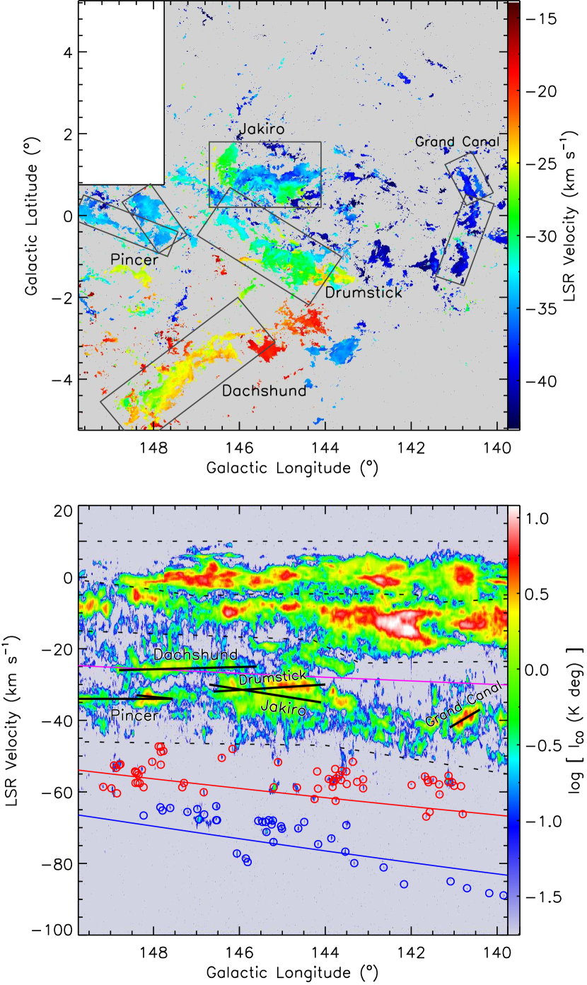
Figure 8: Distribution of the FGMCs on the Perseus Arm. The top panel shows the locations of FGMCs on the ¹²CO velocity-coded map of the Perseus Arm. The bottom panel shows the FGMCs on the longitude-velocity map. The thick black lines present the FGMCs. The black dashed lines divide the regions of the Gould Belt layer, Cam OB1 layer, and Perseus Arm. The red and blue circles indicate the Outer arm clouds (identified by Du et al. 2016) and the New Arm clouds (identified by Sun et al. 2015 and Du et al. 2016). The red and blue lines presented the projections of the Outer Arm spiral (fitted by Du et al. 2016) and the New Arm spiral (fitted by Sun et al. 2015), respectively. The magenta line indicates the projection of the Perseus Arm spiral fitted by Reid et al. (2014).

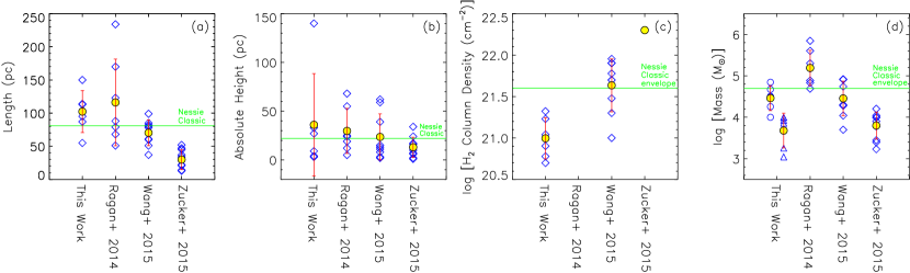
Figure 9: Comparisons of the (a) length, (b) absolute height, (c) mean H₂ column density, and (d) mass of the FGMCs with other works. The yellow filled circle indicates the mean value of each work. The standard deviation is marked by the red error bar. The green line in each panel indicates the value of “Nessie” (Jackson et al. 2010; Goodman et al. 2014), in panel (a) and (b) it indicates the value of “Nessie Classic”, and in panel (c) and (d) it indicates the value of the envelope of “Nessie Classic” traced by HNC. Note that: (1) In panel (c), the H₂ column densities of “This Work”, “Wang+ 2015”, and “Zucker+ 2015” are from ¹³CO derived result, SED fitting result, and an assumed value, respectively; (2) In panel (d), The blue circles and triangles of “This work” indicate the masses derived by ¹²CO and ¹³CO, respectively. In addition, the masses of “Ragan+ 2014”, “Wang+ 2015”, and “Zucker+ 2015” are derived by ¹³CO data, SED fitting column density, and assumed column density, respectively.

The estimation of all the physical parameters is similar to the method presented in Section 3. The only difference is that we do not define masks in this section. Namely, the area where we calculate ¹²CO-derived mass also includes the area where ¹³CO and C¹⁸O emission exists, and similarly for the area where we calculate ¹³CO-derived mass. The calculation methods for all the parameters are as follows.

First, we respectively integrate the ¹²CO, ¹³CO, and C¹⁸O FITS cube of each FGMC over the velocity range that is listed in Table 5. The integrated threshold is also $3\sigma$, and the pixels without signals in the final integrated map are set to be NULL. Then, we adopt “the total number of pixels that are not NULL” $\times$ “the angular area of each pixel” as the total angular area. According to the distance (2.1 kpc), the physical area can be easily estimated. Second, the length is adopted as the physical length of the longer side of the box that confines the FGMCs shown in the top panel of Figure 8. The width is obtained by dividing the physical area by the physical length. Then, the length-to-width ratio can be calculated accordingly. Third, the excitation temperature is calculated by the ¹²CO peak main-beam temperature, and the calculation method is the same as in Equation 2. Fourth, the H₂ column density is also estimated by two methods. For the area traced by ¹²CO, the X-factor method is adopted, and the calculation method is the same as in Equation 3; for the area traced by ¹³CO and C¹⁸O, the LTE method is adopted, and the calculation method is the same as in Equation 4 – 9. Fifth, the calculation method of mass traced by different CO molecules is the same as in Equation 10. Finally, we consider C¹⁸O tracing the dense gas and define the DGMF as the ratio of the molecular mass derived by C¹⁸O to the one derived by ¹³CO.

Generally, on morphology, these FGMCs are (i) at the scale length of $\sim 100$ pc, and (ii) at the scale width of $\sim 10$ pc and $\sim 1$ pc traced by ¹²CO and ¹³CO  respectively. On distribution, (i) except for “Dachshund”, the other FGMCs all distribute near the Galactic plane (the absolute hight $\sim 10$ pc), and (ii) the FP angle range is as large as from $\sim 0$^∘to $\sim 90$^∘; On physical property, (i) their excitation temperature is similar ($\sim 10$ K), (ii) the DGMF range is large ($\sim 0\%-9\%$), (iii) 3 FGMCs have relatively obvious velocity gradients (details in Section 5.2), (iv) the mean H₂ column densities are not high (the densities derived by ¹²CO, ¹³CO  and C¹⁸O are all $\sim 10^{21}$ cm^-2), and (v) the masses derived by ¹²CO are all at the giant molecular cloud (GMC) scale.

The properties of these FGMCs are somewhat different from those of the giant filamentary IRDC “Nessie”. Their lengths are similar to “Nessie Classic” (namely, the part identified by Jackson et al. 2010), but their widths are $\sim 10-100$ times larger than that of “Nessie”. In addition, their mean H₂ column densities are lower than that of “Nessie” for one order of magnitude. However, the properties between the FGMCs traced by ¹³CO and the envelope of “Nessie Classic” traced by HNC (Goodman et al., 2014) are not very different: their width scale is similar, and also they share the same H₂ column density scale of $10^{21}$ cm^-2.

In recent years, using the infrared and molecular line data, Ragan et al. (2014), Wang et al. (2015) and Zucker et al. (2015) have all systematically identified and studied several giant filamentary clouds. Figure 9 shows the comparisons of length, absolute height (namely, the absolute distance to the Galactic plane), H₂ column density, and mass between this work and theirs as well as “Nessie”. Detailed description about the figure is presented in the note. One can see that the lengths, masses derived by ¹²CO and the absolute heights of this work are similar to those of others, while the H₂ column densities are relatively lower than in other works.

5.2 Individuals

5.2.1 “Grand Canal”

The FGMC “Grand Canal” is named after a famous canal in China — the Beijing–Hangzhou Grand Canal, which is the longest and one of the oldest man-made rivers in the world. Unlike other large rivers in China, the Beijing–Hangzhou Grand Canal is a south–north direction river, similar to the FGMC “Crand Canal”, which is almost vertical to the Galactic plane (FP angle $\sim 81$^∘). Using a CO tracer, a point position of this FGMC was first detected by Blitz et al. (1982) with the name of BFS27. In the study of Digel et al. (1996), “Crand Canal” was completely detected and was divided into 3 parts (numbers of 50 – 52 in their catalog, and BFS27 is located at Number 52). Here using relatively highly sensitive and high-resolution data, we consider those three clouds as one filamentary structure and study it again in this section.

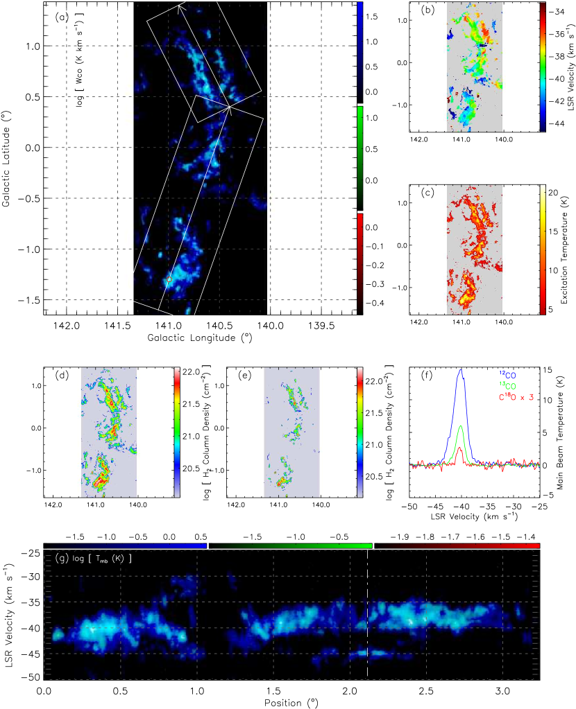
Figure 11: Properties of the FGMC “Grand Canal”. (a) is the integrated intensity map of ¹²CO (blue), ¹³CO (green) and C¹⁸O (red). Note that the value is logarithmic. The red circle indicates the location where C¹⁸O peak main-beam temperature is the highest. (b) is the ¹²CO velocity-coded map. (c) is the excitation temperature map derived by ¹²CO(̇d) and (e) are H₂ column density map derived by ¹²CO and ¹³CO, respectively. Note that the value is logarithmic. (f) is the averaged spectrum of ¹²CO (blue), ¹³CO (green) and C¹⁸O (red) of 9 pixels of the red circle in panel (a). Note that the C¹⁸O spectrum is multiplied by 3. (g) is the average velocity-position map of the white rectangles in panel (a), and the white arrows in panel (a) indicate the position direction. Note that the white pecked line in panel (g) refers to the turning point in panel (a).

Figure 11 presents the properties of this FGMC. From panel (a), one can see that the C¹⁸O distribution is clumpy. These C¹⁸O clumps are located at $(l,b)\cong(140.6,0.6)$^∘, $(140.5,-0.2)$^∘, $(140.9,-0.7)$^∘, and $(141.0,-1.3)$^∘, where the excitation temperature and H₂ column density are relatively higher, as shown in panel (c), (d) and (e). Among them, at the position of $(l,b)\cong(141.0,-1.3)$^∘(which is also the position near BFS27), the C¹⁸O main-beam temperature is the highest, and the three molecular line profiles at this position are shown in panel (f). In addition, the FGMC breaks at the position of $(l,b)\sim(140.75,-0.4)$^∘, and bends at the position of $(l,b)\sim(140.5,0.4)$^∘. North of $b\sim 0.4$^∘, the FGMC splits into two parallel parts with different velocity components, which can be seen in panels (b) and (g). Moreover, from panels (b) and (g), one can see that the FGMC presents a weak velocity gradient along the major axis. In panel (g), at the position of 0^∘ its velocity $\sim-41$ km s^-1, while at the position of 3.3^∘ the velocity becomes to $\sim-37$ km s^-1. Thus, we can roughly estimate that the velocity gradient is $\sim 0.04$ km s^-1 pc^-1.

Compared to other FGMCs, (i) its ¹²CO length-to-width ratio is the highest; (ii) its H₂ column densities derived by ¹²CO, ¹³CO, and C¹⁸O are all the highest; (iii) its excitation temperatures are the highest; and (iv) it is the only FGMC of which the C¹⁸O distribution is clumpy.

5.2.2 “Jakiro”

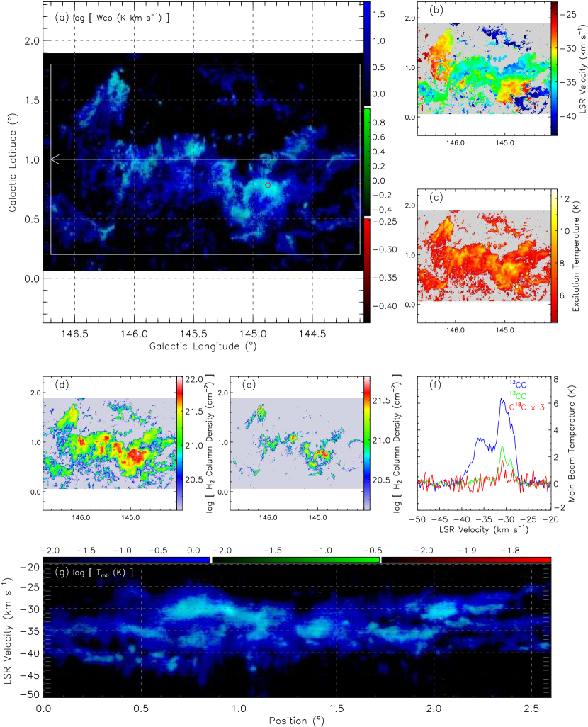
Figure 12: Properties of the FGMC “Jakiro”. The meaning of each panel is consistent with Figure 11.

The FGMC “Jackiro” is named after its complicated velocity components, just as shown in panels (b), (f), and (g) of Figure 12. Figure 10 shows its channel map. One can see that this FGMC seems to be composed of two “S” shapes that twist together, while the ¹³CO seems to be mainly distributed in one of the “S” shapes, just as shown in panel (e) of Figure 12. In addition, C¹⁸O distribution is very diffused.

Compared to other FGMCs, (i) it is the only one which is located above the Galactic plane; (ii) its ¹²CO length to width ratio is the lowest; and (iii) its physical areas and masses traced and derived by ¹²CO and ¹³CO are both the largest.

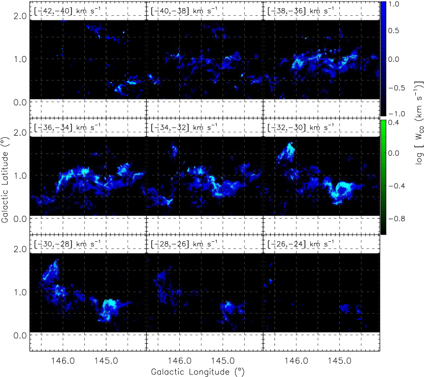
Figure 10: Channel map of ¹²CO (blue) and ¹³CO (green) of FGMC “Jakiro”. Note that the integrated intensity value is logarithmic.

5.2.3 “Drumstick”

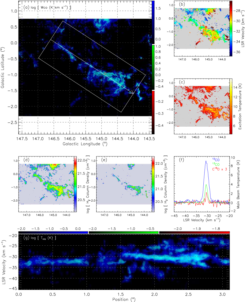
Figure 13: Properties of the FGMC “Drumstick”. The meaning of each panel is consistent with Figure 11.

The FGMC “Drumstick” is named after its shape — one narrower part at the northeast side and one wider part at the southwest side, as shown in Figure 13. These two parts break at the position of $(l,b)\sim(145.8,-0.4)$. The wider part contains more complicated velocity components. As shown in panel (g) of Figure 13, the wider part is composed of about four velocity components: the main component is at the major axis with velocity $\sim-30$ km s^-1, and the other three components distribute at both sides of the main one with velocity $\sim-35$, $-28$, and $-23$ km s^-1, respectively. In addition, this FGMC presents a weak velocity gradient along the major axis. At the position of 0^∘, its velocity $\sim-33$ km s^-1, and at the position of 3.1^∘, the velocity becomes $\sim-30$ km s^-1. Thus, the velocity gradient is $\sim 0.03$ km s^-1 pc^-1. The excitation temperature and H₂ column density of the wider part are more higher than those of the narrower part. The C¹⁸O distribution is relatively diffused in this FGMC, and almost all the C¹⁸O distributes at the wider part.

5.2.4 “Pincer”

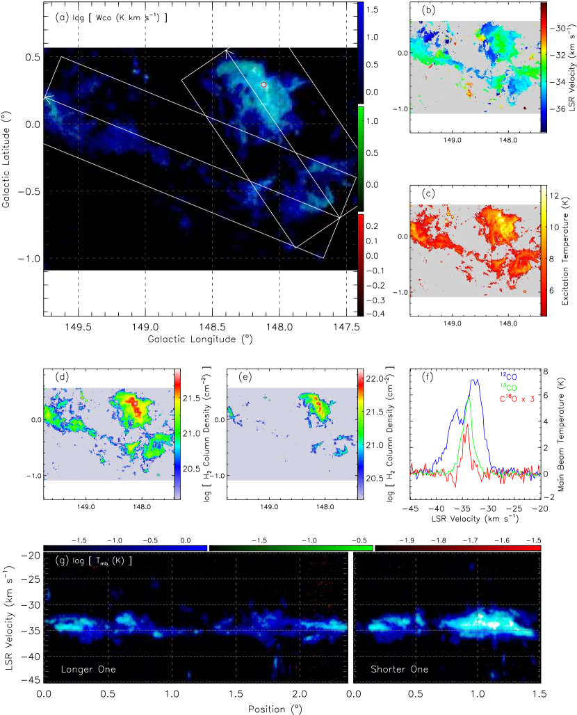
Figure 14: Properties of the FGMC “Pincer”. The meaning of each panel is consistent with Figure 11. Note that in panel (g), the left map and right map refer to the velocity-position maps of “Pincer-longer” and “Pincer-shorter”, respectively.

The FGMC “Pincer” consists of two filamentary structures — the “Pincer-longer” and the “Pincer-shorter”. Those two parts present very different properties, as shown in Figure 14. “Pincer-longer” is very diffused. The ¹³CO on it is even too diffused to form a complete filamentary structure. The C¹⁸O is also rare. The H₂ column density and excitation temperature are both very low. On the other hand, “Pincer-shorter” is more compact, and its H₂ column density and excitation temperature are both higher. The C¹⁸O is rich and largely concentrated in the vicinity of $(l,b)\sim(148.1,0.3)$^∘, where its excitation temperature is relatively higher.

Compared to other FGMCs, (i) this FGMC is the only one that consists of two filamentary components; (ii) the ¹³CO and C¹⁸O on the “Pincer-shorter” are the richest; and (iii) the DGMF of “Pincer-shorter” is the highest.

5.2.5 “Dachshund”

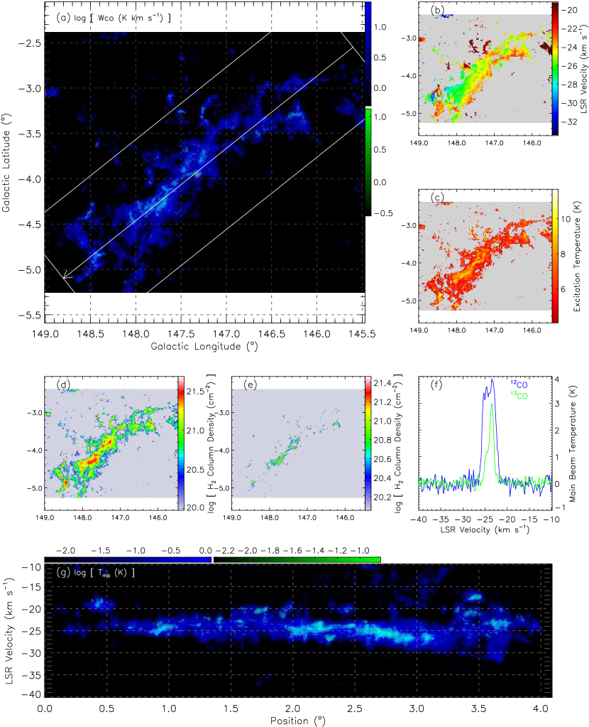
Figure 15: Properties of the FGMC “Dachshund”. The meaning of each panel is consistent with Figure 11. Note that C¹⁸O is not plotted since it is too weak to be detected. And correspondingly the red circle in panel (a) indicates the location where ¹³CO peak main-beam temperature is the highest.

The shape of FGMC “Dachshund” is interesting. It looks like a dog running from the northwest to the southeast, as shown in Figure 15. This FGMC is a very diffused cloud. The C¹⁸O is too weak to be detected. In addition, its excitation temperature is also very low. However, it is noticeable that along its minor axis it presents an obvious velocity gradient. At the “belly” of the dog, the velocity is $\sim-23$ km s^-1, and at the “back” of the dog, it becomes $\sim-27$ km s^-1. Thus, the velocity gradient is estimated to be $\sim 0.25$ km s^-1pc^-1.

Compared to other FGMCs, (i) its height is the largest, namely, it is located farthest away from the Galactic plane; (ii) it is the longest FGMC; and (iii) its DGMF is $\sim 0$ because no C¹⁸O is detected.

5.3 Relations between FGMCs and Galactic Structure

The spiral arms of many galaxies are not smooth (Weaver, 1970). On the arms there exist the so-called substructures, such as the branch, spur, and feather (e.g., Lynds 1970; Piddington 1973; Elmegreen 1980; La Vigne et al. 2006). In the study of 7 galaxies, Elmegreen (1980) has found that the width and length of the spur structure are at the order of magnitude of 100 pc and 1 kpc, respectively. In fact, the substructures of our galaxy were also observed and studied early on (e.g., Sofue 1976; Rickard & Cronyn 1979). Recently, a spur with kpc-length between the Local Arm and the Sagittarius Arm has been identified by Xu et al. (2016), which further implies the complicated situation of the MW substructures.

Apparently, those substructures are also filamentary. However, they are hugely longer and wider than the FGMCs and other giant filamentary clouds studied by Ragan et al. (2014), Wang et al. (2015) and Zucker et al. (2015). In addition, up to now the longest giant filamentary cloud in the MW is just $\sim 500$ pc long (Li et al., 2013). Such FGMCs are indeed too small compared to the substructures like the spur. On the other hand, they are about 10 times larger than the traditional Gould Belt filaments studied by André et al. (2014). Table 4 lists a comparison among several filamentary structures with different scales. There seems to exist a delicate trend in angle (FP angle or pitch angle) such that the angle range and value become small as the filamentary structure becomes large. In addition, their locations also change from subarm to major arm and then to interarm. As mentioned at the beginning of Section 5, the relations between such a giant filament and MW large scale-structure are under research. Some subtle trends have indeed been found (e.g., Ragan et al. 2014), but strong evidences still need more observational samples.

Table 4: Comparison of Filamentary Structure

Structure	Length	Angle	Location	Ref
Gould Belt filament	$1-10$ pc	-	sub-arm	1
FGMC	$\sim 100$ pc	$0-90$∘	major arm	-
Other giant filament	$\sim 100$ pc	$0-70$∘	major&inter arm	2
Feather	$\sim 1$ kpc	$\sim 50$∘	major arm	3,4
Spur	$\sim 1$ kpc	$\sim 60$∘	inter-arm	4,5
Local arm	$>5$ kpc	$\sim 11$∘	-	6,7
Major arm of MW	$>10$ kpc	$7-20$∘	-	7,8

Note. — 1: André et al. (2014);

2: Ragan et al. (2014), Wang et al. (2015),

and Zucker et al. (2015);

3: Lynds (1970);

4: La Vigne et al. (2006);

5: Elmegreen (1980);

6: Xu et al. (2013, 2016);

7: Reid et al. (2014);

8: Steiman-Cameron (2010), Sun et al. (2015),

and Du et al. (2016).

Note that the angle of “FGMC” and “Other giant filament”

refers to the angle between filamentary structure and the

Galactic plane; While the angle in other rows refers to the

pitch angle.

6 Summary

The G140 Region, namely, the Galactic region of $l=[139.75,149.75]^{\circ}$, $b=[-5.25,5.25]^{\circ}$, is one of the target survey areas of the ongoing Milky Way Imaging Scroll Painting (MWISP) project. The ¹²CO ($1-0$), ¹³CO ($1-0$) and C¹⁸O ($1-0$) lines were observed simultaneously using the Purple Mountain Observatory Delingha (PMODLH) 13.7 m telescope. With nearly 2 yr of observations, this region has been completely covered. We take a 96-square-degree part of this region to mainly study the molecular structure of the Local Arm and Perseus Arm. Combining the H I data and part of the Outer Arm results, the gas distribution, warp and flare are discussed. In addition, five filamentary giant molecular clouds (FGMCs) on the Perseus Arm are identified, and their relations to the MW large scale structure are discussed. The main results of the G140 Region are as the follows:

(1) The Local Arm consists of two layers — the Gould Belt layer and the Cam OB1 layer. Their molecular masses are $\sim 2.2\times 10^{3}$ M_⊙ and $\sim 12.7\times 10^{4}$ M_⊙, respectively. In total the Local Arm molecular mass is $\sim 12.9\times 10^{4}$ M_⊙. The Perseus Arm molecular mass is $\sim 28.9\times 10^{4}$ M_⊙.

(2) The mass ratios of H₂ to H I gas on the Local Arm, Perseus Arm, and Outer Arm are 0.36, 0.08, and 0.02, respectively. However, the ratio of Local arm may be overestimated since the H I gas on Local arm is largely underestimated.

(3) The H₂ gas thicknesses of Local arm, Perseus arm, and Outer arm are 117 pc, 149 pc, and 60 pc, respectively; the H I gas thicknesses of the three arms are 220 pc, 291 pc, and 550 pc, respectively. The H₂ gas height of the three arms are 18 pc, -16 pc, and 170 pc, respectively; the H I gas height of the three arms are -2 pc, -19 pc, and 160 pc, respectively. It can be seen that the warp structure of both atomic and molecular gas is obvious, while the flare structure only exists in atomic gas.

(4) Five FGMCs with lengths $\sim 100$ pc on the Perseus Arm are identified, among which four are newly identified. Their masses derived by ¹²CO, ¹³CO, and C¹⁸O are $\sim 10^{4}$ M_⊙, $\sim 10^{3}$ M_⊙, $\sim 10^{2}$ M_⊙, respectively; and their mean H₂ column densities derived by ¹²CO, ¹³CO and C¹⁸O are all $\sim 10^{21}$ cm^-2.

Table 5: Properties of FGMCs

Name			(1)	Grand	Jakiro	Drumstick	Pincer	Pincer	Dachshund
				Canal			-longer	-shorter
Glon		(∘)	(2)	140.6	145.4	145.3	148.7	148.0	147.2
Glat		(∘)	(3)	-0.1	0.9	-0.8	-0.3	-0.1	-3.8
FP Angle		(∘)	(4)	81	0	33	22	56	39
Height		(pc)	(5)	-4	33	-27	-9	-3	-140
$T_{\mathrm{ex}}$		(K)	(6)	9/26	7/16	8/16	6/12	7/21	6/12
DGMF		(%)	(7)	3.2	0.1	0.8	0.7	8.7	0
12CO	$V_{\mathrm{LSR}}$	(km s-1)	(8)	[-45,-33]	[-43,-23]	[-37,-26]	[-38,-29]	[-38,-29]	[-34,-19]
	Scale	(pc$\times$pc)	(9)	$113\times 9$	$95\times 31$	$114\times 19$	$87\times 10$	$55\times 15$	$150\times 16$
	Len/Wid		(10)	13	3	6	9	4	9
	Area	(pc2)	(11)	991	2918	2115	848	847	2389
	$N_{\mathrm{H_{2}}}$	($10^{21}$cm-2)	(12)	1.9/11.6	1.5/10.1	1.4/7.3	0.7/3.3	1.3/8.1	0.8/4.0
	Mass	(104M⊙)	(13)	3.1	7.0	4.7	1.0	1.8	3.2
13CO	$V_{\mathrm{LSR}}$	(km s-1)	(14)	[-45,-34]	[-41,-25]	[-36,-27]	[-37,-30]	[-37,-30]	[-30,-20]
	Scale	(pc$\times$pc)	(14)	$113\times 3$	$95\times 8$	$114\times 6$	-	$55\times 7$	$120\times 2$
	Len/Wid		(15)	37	13	20	-	8	58
	Area	(pc2)	(16)	341	722	663	142	359	248
	$N_{\mathrm{H_{2}}}$	($10^{21}$cm-2)	(17)	2.1/16.4	0.8/6.3	1.1/5.0	0.6/2.7	1.7/21.9	0.5/2.9
	Mass	(103M⊙)	(18)	11.4	9.8	11.5	1.4	10.0	2.1
C18O	$V_{\mathrm{LSR}}$	(km s-1)	(19)	[-43,-36]	[-32,-28]	[-34,-29]	[-37,-31]	[-37,-31]	-
	Area	(pc2)	(20)	4.3	0.3	2.1	0.2	12.9	-
	$N_{\mathrm{H_{2}}}$	($10^{21}$cm-2)	(21)	5.3/12.8	2.3/2.6	2.8/4.7	2.7/3.1	4.2/12.2	-
	Mass	(102M⊙)	(22)	3.6	0.1	0.9	0.1	8.7	-

Note. — Row (1): the name of FGMC. Row (2) – (3): the central position of FGMC in Galactic coordinate. Row (4): the angle between the longer side of FGMC and the Galactic plane. Row (5): the height to the Galactic plane, which is calculated by height = distance $\times$ $\sin$(latitude). Row (6): mean/max excitation temperature of FGMC. Row (7): dense gas mass function of FGMC. Row (8) – (13): parameters traced or derived by ¹²CO, respectively are LSR velocity range, length $\times$ width, ratio of length to width, area, mean/max H₂ column density, and mass. Row (14) – (18) and Row (19) – (22): parameters traced or derived by ¹³CO and C¹⁸O, respectively. And the meaning of each row is consistent with Row ¹²CO. Note that Row (14) – (15) of “Pincer-longer” and Row (19) – (22) of “Dachshund” are null because of the weak emission.

References

- Abdo et al. (2010) Abdo, A. A. et al. 2010, ApJ, 710, 133
- André et al. (2014) André, P., Di Francesco, J., Ward-Thompson, D., et al. 2014, Protostars and Planets VI, 27
- Arp (1966) Arp, H. 1966, Atlas of Peculiar Galaxies, Pasadena: California Inst. Technology
- Asaki et al. (2010) Asaki, Y., Deguchi, S., Imai, H., et al. 2010, ApJ, 721, 267
- Battersby & Bally (2014) Battersby, C., & Bally, J. 2014, The Labyrinth of Star Formation, 36, 417
- Binney (1978) Binney, J. 1978, MNRAS, 183, 779
- Binney (1992) Binney, J. 1992, ARA&A, 30, 51
- Blitz et al. (1982) Blitz, L., Fich, M., & Stark, A. A. 1982, ApJS, 49, 183
- Bok (1959) Bok, B. J., 1959, The Observatory, 79, 58
- Bourke et al. (1997) Bourke, T. L., Garay, G., Lehtinen, K. K., et al. 1997, ApJ, 476, 781
- Burke (1957) Burke, B. F. 1957, AJ, 62, 90
- Burton et al. (1975) Burton, W. B., Gordon, M. A., Bania, T. M., & Lockman, F. J. 1975, ApJ, 202, 30
- Castets & Langer (1995) Castets, A., & Langer, W. D. 1995, A&A, 294, 835
- Dame et al. (2001) Dame, T. M., Hartmann, D., & Thaddeus, P. 2001, ApJ, 547, 792
- Dame & Thaddeus (2011) Dame, T. M., & Thaddeus, P. 2011, ApJL, 734, L24
- Dehnen (1998) Dehnen, W. 1998, AJ, 115, 2384
- Digel et al. (1996) Digel, S. W., Lyder, D. A., Philbrick, A. J., Puche, D., & Thaddeus, P. 1996, ApJ, 458, 561
- Djorgovski & Sosin (1989) Djorgovski, S., & Sosin, C. 1989, ApJL, 341, L13
- Du et al. (2016) Du, X., Xu, Y., Yang, J., et al. 2016, ApJS, 224, 7
- Duarte-Cabral et al. (2015) Duarte-Cabral, A., Acreman, D. M., Dobbs, C. L., et al. 2015, MNRAS, 447, 2144
- Elmegreen (1980) Elmegreen, D. M. 1980, ApJ, 242, 528
- Ferking et al. (1982) Frerking, M. A., Langer, W. D., & Wilson, R. W. 1982, ApJ, 262, 590
- Freudenreich et al. (1994) Freudenreich, H. T., Berriman, G. B., Dwek, E., et al. 1994, ApJL, 429, L69
- García-Ruiz et al. (2002) García-Ruiz, I., Sancisi, R., & Kuijken, K. 2002, A&A, 394, 769
- Georgelin & Georgelin (1976) Georgelin, Y. M., & Georgelin, Y. P. 1976, A&A, 49, 57
- Grenier (2004) Grenier, I. A. 2004, arXiv:astro-ph/0409096
- Goodman et al. (2014) Goodman, A. A., Alves, J., Beaumont, C. N., et al. 2014, ApJ, 797, 53
- Heyer et al. (1998) Heyer, M. H., Brunt, C., Snell, R. L., et al. 1998, ApJS, 115, 241
- Heyer & Dame (2015) Heyer, M., & Dame, T. M. 2015, ARA&A, 53, 583
- Hildebrand (1983) Hildebrand, R. H. 1983, QJRAS, 24, 267
- Honig & Reid (2015) Honig, Z. N., & Reid, M. J. 2015, ApJ, 800, 53
- Hou & Han (2014) Hou, L. G., & Han, J. L. 2014, A&A, 569, A125
- Huchtmeier et al. (1980) Huchtmeier, W. K., Seiradakis, J. H., & Tammann, G. A. 1980, A&A, 89, 95
- Humphreys (1978) Humphreys, R. M. 1978, ApJS, 38, 309
- Jackson et al. (2010) Jackson, J. M., Finn, S. C., ChambersE. T., Rathborne, J. M., Simon, R., 2010, ApJ, 719, L185
- Kalberla et al. (2007) Kalberla, P. M. W., Dedes, L., Kerp, J., & Haud, U. 2007, A&A, 469, 511
- Kalberla & Kerp (2009) Kalberla, P. M. W., & Kerp, J. 2009, ARA&A, 47, 27
- Kerr (1957) Kerr, F. J. 1957, AJ, 62, 93
- Kerr et al. (1957) Kerr, F. J., Hindman, J. V., & Carpenter, M. S. 1957, Nature, 180, 677
- La Vigne et al. (2006) La Vigne, M. A., Vogel, S. N., & Ostriker, E. C. 2006, ApJ, 650, 818
- Levine et al. (2006) Levine, E. S., Blitz, L., & Heiles, C. 2006, ApJ, 643, 881
- Li et al. (2013) Li G.-X., Wyrowski F., Menten K., Belloche A., 2013, A&A, 559, A34
- Lindblad (1967) Lindblad, P. O. 1967, BAN, 19, 34
- Lyder (2001) Lyder, D. A. 2001, AJ, 122, 2634
- Lynds (1970) Lynds, B. T. 1970, in IAU Symp. 38, The Spiral Structure of Our Galaxy, ed. W. Becker & G. I. Contopouplos (Dordrecht: Reidel), 26
- Miyamoto et al. (1988) Miyamoto, M., Yoshizawa, M., & Suzuki, S. 1988, A&A, 194, 107
- Momany et al. (2006) Momany, Y., Zaggia, S., Gilmore, G., et al. 2006, A&A, 451, 515
- Nakanishi & Sofue (2003) Nakanishi, H., & Sofue, Y. 2003, PASJ, 55, 191
- Oort et al. (1958) Oort, J. H., Kerr, F. J., Westerhout, G. 1958, MNRAS, 118, 379
- Piddington (1973) Piddington, J. H. 1973, ApJ, 179, 755
- Pineda et al. (2010) Pineda, J. L., Goldsmith, P. F., Chapman, N., et al. 2010, ApJ, 721, 686
- Ragan et al. (2014) Ragan, S. E., Henning, T., Tackenberg, J., Beuther, H., Johnston, K. G., Kainulainen, J., Linz, H., 2014, A&A, 568, A73
- Reid et al. (2014) Reid, M. J. et al. 2014, ApJ, 783, 130
- Rickard & Cronyn (1979) Rickard, J. J., & Cronyn, W. M. 1979, ApJ, 228, 755
- Sancisi (1976) Sancisi, R. 1976, A&A, 53, 159
- Sandage (1961) Sandage, A. 1961, The Hubble Atlas of Galaxies, Washington: Carnegie Institution
- Shan et al. (2012) Shan, W.L., Yang, J., Shi, S. C., et al. 2012, IEEE Transactions on Terahertz Science and Technology, 2,593
- Sodroski et al. (1987) Sodroski, T. J., Dwek, E., Hauser, M. G., & Kerr, F. J. 1987, ApJ, 322, 101
- Sofue (1976) Sofue, Y. 1976, A&A, 48, 1
- Steiman-Cameron (2010) Steiman-Cameron, T. Y. 2010, Galaxies and their Masks, 45
- Straižys et al. (2001) Straižys, V., Černis, K., & Bartašiute, S. 2001, A&A, 374, 288
- Straižys & Laugalys (2007) Straižys, V., & Laugalys, V. 2007, Baltic Astronomy, 16, 167
- Straižys & Laugalys (2008) Straižys, V., & Laugalys, V. 2008, Handbook of Star Forming Regions, Volume I, 4, 294
- Strauss et al. (1979) Strauss, F. M., Vieira, E. R., & Poeppel, W. G. L. 1979, A&A, 71, 319
- Su et al. (2016) Su, Y., Sun, Y., Li, C., et al. 2016, ApJ, 828, 59
- Sun et al. (2015) Sun, Y., Xu, Y., Yang, J., et al. 2015, ApJL, 798, L27
- Russeil et al. (2007) Russeil, D., Adami, C., & Georgelin, Y. M. 2007, A&A, 470, 161
- Tackenberg et al. (2013) Tackenberg J., Beuther H., Plume R., Henning T., Stil J., Walmsley M., Schuller F., Schmiedeke A., 2013, A&A, 550, A116
- Taylor et al. (2003) Taylor, A. R., Gibson, S. J., Peracaula, M., et al. 2003, AJ, 125, 3145
- Vallée (2008) Vallée, J. P. 2008, AJ, 135, 1301
- Wang et al. (2015) Wang, K., Testi, L., Ginsburg, A., et al. 2015, MNRAS, 450, 4043
- Weaver (1970) Weaver, H. 1970, in IAU Symp. 39, Interstellar Gas Dynamics, ed. H. J. Habing (Dordrecht: Kluwer), 22
- westerhout (1957) Westerhout, G. 1957, Bull. Astron. Inst. Netherlands, 13, 201
- Wouterloot et al. (1990) Wouterloot, J. G. A., Brand, J., Burton, W. B., & Kwee, K. K. 1990, A&A, 230, 21
- Xu et al. (2013) Xu, Y., Li, J. J., Reid, M. J., et al. 2013, ApJ, 769, 15
- Xu et al. (2016) Xu, Y., Reid, M., Dame, T., et al. 2016, arXiv:1610.00242
- Xu et al. (2006) Xu, Y., Reid, M. J., Zheng, X. W., & Menten, K. M. 2006, Science, 311, 54
- Zdanavičius et al. (2005) Zdanavičius, J., Zdanavičius, K., & Straižys, V. 2005, Baltic Astronomy, 14, 31
- Zucker et al. (2015) Zucker, C., Battersby, C., & Goodman, A. 2015, ApJ, 815, 23