A parallelizable augmented Lagrangian method applied to large-scale non-convex-constrained optimization problems

Abstract

We contribute improvements to a Lagrangian dual solution approach applied to large-scale optimization problems whose objective functions are convex, continuously differentiable and possibly nonlinear, while the non-relaxed constraint set is compact but not necessarily convex. Such problems arise, for example, in the split-variable deterministic reformulation of stochastic mixed-integer optimization problems. The dual solution approach needs to address the nonconvexity of the non-relaxed constraint set while being efficiently implementable in parallel. We adapt the augmented Lagrangian method framework to address the presence of nonconvexity in the non-relaxed constraint set and the need for efficient parallelization. The development of our approach is most naturally compared with the development of proximal bundle methods and especially with their use of serious step conditions. However, deviations from these developments allow for an improvement in efficiency with which parallelization can be utilized. Pivotal in our modification to the augmented Lagrangian method is the use of an integration of approaches based on the simplicial decomposition method (SDM) and the nonlinear block Gauss-Seidel (GS) method. An adaptation of a serious step condition associated with proximal bundle methods allows for the approximation tolerance to be automatically adjusted. Under mild conditions optimal dual convergence is proven, and we report computational results on test instances from the stochastic optimization literature. We demonstrate improvement in parallel speedup over a baseline parallel approach.

1 Introduction and Background

We develop a dual solution approach to the problem of interest having the form

$$\zeta^{*}:=\min_{x,z}\left\{f(x):Qx=z,x\in X,z\in Z\right\},$$ (1)

where $f$ is convex and continuously differentiable, $Q\in\mathbb{R}^{q\times n}$ is a block-diagonal matrix determining linear constraints $Qx=z$, $X\subset\mathbb{R}^{n}$ is a closed and bounded set, and $Z\subset\mathbb{R}^{q}$ is a linear subspace. The vector $x\in X$ of decision variables is derived from the original decisions associated with a problem, while the vector $z\in Z$ of auxiliary variables are introduced to effect a decomposable structure in (1). The block diagonal components of $Q$ are denoted $Q_{i}\in\mathbb{R}^{q_{i}\times n_{i}}$, $i=1,\dots,m$. Problem (1) is general enough to subsume, for example, the split-variable deterministic reformulation of a stochastic optimization problem with potentially multiple stages, as defined, for example, in BirgeLouveaux2011 , while it can also model the case where $f$ is nonlinear (and convex) and/or $X$ is any compact (but not necessarily convex) set.

The Lagrangian dual function resulting from the relaxation of $Qx=z$ is

$$\phi(\omega):=\min_{x,z}\left\{f(x)+\omega^{\top}(Qx-z),x\in X,z\in Z\right\}.$$ (2)

Given that $X$ is compact and $f$ is continuous, in order for $-\infty<\phi(\omega)$ to hold, it is necessary and sufficient that the following dual feasibility assumption be maintained:

$$\omega\in Z^{\perp}:=\left\{\upsilon\in\mathbb{R}^{q}:\upsilon^{\top}z=0\;\text{for all}\;z\in Z\right\},$$ (3)

either by assumption or by construction. Under condition (3), the $z$ term in definition (2) vanishes, and we may compute $\phi(\omega)=\min_{x}\left\{f(x)+\omega^{\top}Qx:x\in X\right\}.$ Consequently, $\phi$ becomes separable as

$$\phi(\omega)=\sum_{i=1}^{m}\phi_{i}(\omega_{i})$$

where $\phi_{i}(\omega_{i}):=\min_{x}\left\{f_{i}(x_{i})+\omega_{i}^{\top}Q_{i}x_{i}:x_{i}\in X_{i}\right\}$ and $\omega=(\omega_{1},\dots,\omega_{m})\in\mathbb{R}^{q_{1}}\times\cdots\times\mathbb{R}^{q_{m}}$ has a block structure compatible with the block diagonal structure of $Q$. The Lagrangian dual problem is:

$$\zeta^{LD}:=\max_{\omega}\phi(\omega).$$ (4)

In this paper, we develop, analyze, and apply an iterative solution approach to solving problem (4) subject to the following challenges:

Implementability:

The set $X$ is not convex (for example, it may have mixed-integer constraints as part of its definition). Consequently the augmented Lagrangian method is not supported by the theory of proximal point methods.

Efficiency of parallelization:

The solution approach should be amenable to efficient parallel computation, in the sense of maximizing the computational work that can be parallelized, the memory usage that can be distributed, and minimizing the amount of parallel communication.

For the Lagrangian dual problem (4), we note that the objective function $\phi$ is concave, even when $f$ and $X$ are not convex. We can apply a subgradient method (see e.g. Shor1985 ; in textbooks Bertsekas1999 ; Ruszczynski2006 ) for solving (4) in an efficiently parallelizable manner. Such an approach is proposed in caroe1999dual . However, it is preferable to make use of structural features of (4) that allow for smoothing or regularization, so that better convergence properties are realized. For this reason, we consider alternative developments based on proximal point methods that are modified to address both of the above two challenges.

As a starting point, we first consider the classical augmented Lagrangian method based on proximal point methods. The augmented Lagrangian (AL) method (also known as the method of multipliers) is developed from proximal point methods, and references include Hestenes1969 ; Powell1969 ; Bertsekas1982 ; Bertsekas1999 . The AL method typically has favorable convergence properties as a dual solution approach for convex problems (linear convergence rate under certain assumptions, see Rockafellar1976MO ; Bertsekas1982 and references cited therein). However, two issues arise: 1) the set $X$ is not convex, and so current theories of convergence are not applicable; and 2) the primal subproblem associated with each iteration of the AL method is not separable due to the augmented Lagrange term, making efficient parallel implementations difficult to develop.

We introduce modifications to the AL method that address both of these issues. In order to introduce computational tractability in light of the possible nonlinearity of $f$ and the nonconvexity of $X$, the modified AL method solves an alternative dual problem that can provide a weaker dual bound than that provided by the value of (4). In the case when $f$ is linear, the alternative dual problem is equivalent to (4). This matter is explained in more detail in Section 3. The method that results from these modifications is most naturally compared with the proximal bundle method.

The proximal bundle method initially appeared in LemarechalWolfe1975 , and for a survey with history, see OliveiraSagastizabal2014 . Use of inexact oracles for computing $\phi(\omega)$ and elements of the subdifferential set $\partial\phi(\omega)$ are studied in OliveiraSagastizabal2014 ; OliveiraEtAl2014 ; HareEtAl2016 and references therein. In its dual form, the bundle method may be referred to as the stabilized column generation method BenAmor2009SCG or the proximal simplicial decomposition method Bertsekas2015 . In implementation, the developed algorithm more closely resembles the latter dual form.

For parallelization of the proximal bundle method, see FischerHelmberg2014 and LubinEtAl2013 . The approach developed in this paper is most naturally compared with LubinEtAl2013 , as both approaches address the manner in which the same continuous master problem is approximately solved. The approach of FischerHelmberg2014 uses a substantially different parallel computational paradigm based on subspace optimization. This approach, in which solution subspaces are assigned to processors based on periodically updated global state information, is not necessarily based on the problem’s decomposable structure.

The proximal bundle method approach requires modification for efficient parallelization. This matter is addressed in LubinEtAl2013 , where a solution to the continuous master problem is obtained by primal dual interior point methods that exploit the decomposable structure present in the augmented Lagrangian term. We provide and analyze an alternative approach based on the use of:

1. the simplicial decomposition method (SDM) Holloway1974 ; Hohenbalken1977 ; Bertsekas1999 ; Bertsekas2015Text , which provides an alternative framework to the proximal bundle method to address the implementability of the proximal point method while allowing for the possibility that $f$ is nonlinear; and

2. nonlinear block Gauss-Seidel (GS) method Hildreth1957 ; Warga1963 ; GS2000 ; Tseng2001 ; Bonettini2011 to approximate the solutions to the continuous master problem.

Motivated by its constituent parts, the algorithm we develop is referred to as SDM-GS-ALM.

Algorithm SDM-GS-ALM addresses the solution to an alternative dual problem which is equivalent to (4) when $f$ is linear, but in general provides a weaker dual bound otherwise. This dual problem is used to address the more general setting where $f$ is convex but possibly nonlinear.

In an iteration of SDM-GS-ALM, the analog to the continuous master problem is not solved to (near) exactness; instead, approximate solutions based on possibly just one nonlinear block GS iteration are used. Due to the underlying need for convexification of the non-relaxed constraint set, implementability requires that the nonlinear block GS method must be integrated with the SDM so that optimal convergence of the resulting iterations can be established. In this way, a serious step condition similar to that used in proximal bundle methods is eventually satisfied after a finite number of such integrated SDM-GS iterations, and analogous dual optimal convergence of our approach is recovered even with the deviations from the proximal bundle method. In summary, we algorithmically integrate the AL method, the SDM, nonlinear block GS iterations, and the proximal bundle method serious step condition. A convergence analysis is also provided for SDM-GS-ALM. Such an integration allows for a considerable improvement in parallel efficiency with respect to maximizing the computational work that can be parallelized, the memory usage that can be distributed, and minimizing the amount of parallel communication.

Other methods developed in the past that are related to aspects of our contribution include the following. In terms of approximating within the AL method, we include reference to Eckstein2003 ; EcksteinSilva2013 , where the research goal of developing implementable approximation criteria is addressed. The separable augmented Lagrangian (SALA) method Hamdi1997 , which is an application of the alternating direction method of multipliers (ADMM) GlowinskiMarrocco1975 ; GabayMercier1976 ; BoydEtAl2011 with a form of resource allocation decomposition and incorporates separability into the AL method. Other approaches to introducing separability into the AL method include ChatzipanagiotisEtAl2014 ; TappendenEtAl2015 . Jacobi iterate approaches applied within either a proximal bundle method or an AL method framework are considered in MulveyRuszczynski1992 ; Ruszczynski1995 ; the accelerated distributed augmented Lagrangian method (ADAL) developed in ChatzipanagiotisEtAl2014 is like a Jacobi-iterate analogue of ADMM with supporting convergence analysis. Other approaches to incorporating separability are found in the alternating linearization approaches KiwielEtAl1999 ; LinEtAl2014 and the predictor corrector proximal multiplier (PCPM) methods ChenTeboulle1994 ; HeEtAl2002 . All of these methods provide implementable mechanisms for approximating primal subproblem solutions and effecting parallelism in a setting where $X$ is convex. However, they are not practically implementable in our setting where $X$ is not convex and its convex hull $\operatorname{conv}(X)$ is not given beforehand in a computationally useful closed-form description.

Another recently developed algorithm, referred to as FW-PH BolandEtAl2016 , is closely related to the SDM-GS-ALM algorithm developed in this paper. In terms of functionality, both appear as modifications to ADMM with inner approximated subproblem solutions. While the algorithms differ only slightly in terms of functionality, there are substantial differences in the motivation and the convergence analysis. The convergence analysis of FW-PH interfaces with the convergence analysis for ADMM, which is most naturally developed in the context of the theory of maximal monotone operators and Douglas-Rachford splitting methods EcksteinBertsekas1992 ; EcksteinYao2015 , or as the proximal decomposition of the graph of a maximal monotone operator MaheyEtAl1995 . In contrast, the convergence analysis of SDM-GS-ALM naturally reflects its synthesis of SDM, the nonlinear block GS method, the proximal bundle method, and the AL method. The convergence analysis of SDM-GS-ALM follows under more general assumptions than that for FW-PH. In particular, the convergence analysis of SDM-GS-ALM allows for trimming of the inner approximations, and it does not require the warm-starting required by FW-PH. The most important difference in functionality is due to the influence of ideas from proximal bundle methods in SDM-GS-ALM, where updates of $\omega$ are taken conditionally at each iteration, while such updates are taken unconditionally at each iteration of FW-PH. We shall see that these conditional updates help to mitigate performance problems that arise due to the seemingly inevitable use of suboptimal algorithm parameters.

In papers such as GadeEtAl2016 ; FeizollahiEtAl2015 , ADMM is applied directly to the primal problem (1). In both works, it is acknowledged that ADMM is not theoretically supported in optimal convergence due to the lack of convexity of $X$. Nevertheless, GadeEtAl2016 reports the potential for Lagrangian dual bounds to be recovered at each iteration of ADMM even though it is applied to (1). In FeizollahiEtAl2015 , where ADMM is applied to nonconvex decentralized unit commitment problems, heuristic improvements to ADMM are introduced to address the lack of convexity due to the mixed-integer constraints. In contrast to both of these approaches, where ADMM is applied directly to the primal problem (1), the approach developed in this paper, and its related approach BolandEtAl2016 , both resemble ADMM but with application to a primal characterization of the dual problem. In these two approaches, the challenge of not having an explicit form for this primal characterization is addressed.

The remainder of the paper is organized as follows. In Section 2, a general algorithmic framework based on the AL method with approximate subproblem solutions is developed and analyzed. In Section 3, a specific implementation of the Section 2 framework is posed based on the integration of SDM and GS methods, which addresses the aforementioned issues of implementability and efficiency of parallelization. In Section 4, computational experiments and their outcomes are described and interpreted. And at last, Section 5 concludes the paper and provides avenues for future work.

2 An alternative AL approximation approach

In the following development, we address the solution of a slightly different dual problem

$$\zeta^{CLD}:=\max_{\omega\in Z^{\perp}}\phi^{C}(\omega).$$ (5)

based on the dual function $\phi^{C}\left(\omega\right):=\min_{x}\left\{f(x)+\omega^{\top}Qx:x\in\operatorname{conv}(X)\right\}$. The only difference between $\phi^{C}$ and $\phi$ is the use of constraint set $\operatorname{conv}(X)$ in the former versus the use of $X$ in the latter. We assume as before that $\omega\in Z^{\perp}$.

Remark 1

Under the assumption that $\operatorname{conv}(X)$ is not known beforehand by any characterization, direct evaluation of $\phi^{C}$ or any of its subgradients at any $\omega\in Z^{\perp}$ is not possible. This dual function is not used in the proximal bundle method and is only treated indirectly in the current development.

The dual problem (5) has the following primal characterization

$$\zeta^{CLD}=\min_{x,z}\left\{f(x):Qx=z,x\in\operatorname{conv}(X),z\in Z\right\},$$ (6)

where $\operatorname{conv}(X)$ is the convex hull of $X$. In addition to generating a sequence $\left\{\omega^{k}\right\}$ of dual solutions to (5), our algorithm will also generate a sequence of primal solutions $\left\{(x^{k},z^{k})\right\}$ to (6), and so reference to (6) will be useful. In applying the AL method to problem (6), the continuous master problem for fixed $\omega\in Z^{\perp}$ takes the form

$$\zeta_{\rho}^{AL}(\omega):=\min_{x,z}\left\{L_{\rho}(x,z,\omega),x\in\operatorname{conv}(X),z\in Z\right\}$$ (7)

where the augmented Lagrangian (AL) relaxes $Qx=z$ and is defined by

$$L_{\rho}(x,z,\omega):=f(x)+\omega^{\top}Qx+\frac{\rho}{2}\left\|Qx-z\right\|_{2}^{2}.$$ (8)

Lemma 1

For any optimal solution $\omega^{*}$ to problem (5), we have $\zeta_{\rho}^{AL}(\omega^{*})=\zeta^{CLD}$. Additionally, any optimal solution $(x^{*},z^{*})$ to problem (7) with $\omega=\omega^{*}$ is also optimal for problem (6).

Proof

We specialize developments in, e.g., Section 4 of Rockafellar1976ALMethod or Section 6.4.3 of Ruszczynski2006 . Due to the convexity of $f$, $\operatorname{conv}(X)$, and $Z$, we may compute

$$\max_{\omega\in Z^{\perp}}\phi^{C}(\omega)-\frac{1}{2\rho}\left\|\omega-\overline{\omega}\right\|_{2}^{2}$$ (9)

$$=\max_{\omega\in Z^{\perp}}\min_{x}\left\{f(x)+\omega^{\top}Qx-\frac{1}{2\rho}\left\|\omega-\overline{\omega}\right\|_{2}^{2}:x\in\operatorname{conv}(X)\right\}$$

$$=\min_{x}\left\{\begin{array}[]{l}f(x)+\overline{\omega}^{\top}Qx\\ +\max_{\omega\in Z^{\perp}}\left\{(\omega-\overline{\omega})^{\top}Qx-\frac{1}{2\rho}\left\|\omega-\overline{\omega}\right\|_{2}^{2}\right\}:x\in\operatorname{conv}(X)\end{array}\right\}$$ (12)

$$=\min_{x}\left\{f(x)+\overline{\omega}^{\top}Qx+\frac{\rho}{2}\min_{z}\left\{\left\|Qx-z\right\|_{2}^{2}:z\in Z\right\}:x\in\operatorname{conv}(X)\right\}$$

$$=\min_{x,z}\left\{L_{\rho}(x,z,\overline{\omega}),x\in\operatorname{conv}(X),z\in Z\right\}.$$ (13)

The switching of $\min$ and $\max$ is justified by the Sion min-max theorem. In substituting $\overline{\omega}=\omega^{*}$, the value of the left-hand side maximization problem (9) is clearly $\zeta^{CLD}$, while the same substitution on the right-hand side (13) yields the value $\zeta_{\rho}^{AL}(\omega^{*})$, from which we see that $\zeta^{CLD}=\zeta_{\rho}^{AL}(\omega^{*})$. To prove the last claim, we note that $L_{\rho}(x^{*},z^{*},\omega^{*})=\zeta^{CLD}$ implies that $\left\|Qx^{*}-z^{*}\right\|_{2}^{2}=0$. Otherwise, $\phi^{C}(\omega^{*})<\zeta^{CLD}$, contradicting the dual optimality of $\omega^{*}$. Thus, $(x^{*},z^{*})$ is feasible and optimal for problem (6).

It is straightforward from the definitions that $\phi^{C}(\omega)\leq\phi(\omega)$ for all dual feasible $\omega\in Z^{\perp}$. In the case when $f$ is linear, we have $\phi^{C}(\omega)=\phi(\omega)$ for all $\omega\in Z^{\perp}$ and so $\zeta^{LD}=\zeta^{CLD}$. But in the general case where $f$ is nonlinear, the dual (5) can be “weaker” than (4), where $\zeta^{CLD}<\zeta^{LD}$ can occur, which we see in the following example. Let $f:\mathbb{R}^{2}\mapsto\mathbb{R}$ be defined by $f(x)=(x_{1}-0.5)^{2}+(x_{2}-0.5)^{2}$, $X=\left\{0,1\right\}\times\left\{0,1\right\}$, and let $Qx=z$ be defined to model the constraints $x_{1}-z_{1}=0$ and $x_{2}-z_{2}=0$ where $Z=\left\{(z_{1},z_{2}):z_{1}=z_{2}\right\}\subset\mathbb{R}^{2}$. We see trivially that $\zeta^{CLD}=0$, which is verified with the saddle point $x_{1}^{*}=x_{2}^{*}=z_{1}^{*}=z_{2}^{*}=0.5$ and $\omega^{*}=(0,0)$. However, $\zeta^{LD}=0.5$, which is verified with either of the saddle points $x_{1}^{*}=x_{2}^{*}=z_{1}^{*}=z_{2}^{*}=0$ and $\omega^{*}=(0,0)$, or $x_{1}^{*}=x_{2}^{*}=z_{1}^{*}=z_{2}^{*}=1$ and $\omega^{*}=(0,0)$. Thus, $\zeta^{CLD}<\zeta^{LD}$.

In the proximal bundle method, the dual function $\phi$ is approximated by a cutting plane model function which majorizes $\phi$. In the next development, we use the following approximation $\widehat{\phi}:\mathbb{R}^{q}\times\mathbb{R}^{n}\times\mathbb{R}^{q}\mapsto\mathbb{R}$ of $\phi^{C}$ centered at $(x^{k},z^{k})$, $k\geq 0$, in place the cutting plane model:

$$\widehat{\phi}(\omega,x^{k},z^{k}):=L_{\rho}(x^{k},z^{k},\omega)+\frac{\rho}{2}\left\|Qx^{k}-z^{k}\right\|_{2}^{2}.$$

This approximation satisfies the following bounding relationship.

Lemma 2

For each $(x^{k},z^{k})$, $k\geq 0$, such that the $z$-optimality condition is satisfied:

$$z^{k}\in\operatorname*{argmin}_{z}\left\{\left\|Qx^{k}-z\right\|:z\in Z\right\},$$ (14)

we have for each $\omega\in Z^{\perp}$

$$\widehat{\phi}(\omega,x^{k},z^{k})\geq\phi^{C}\left(\omega+\rho(Qx^{k}-z^{k})\right).$$ (15)

Proof

Via convexity of the term $\left\|Qx-z\right\|_{2}^{2}$ over $(x,z)\in\operatorname{conv}(X)\times Z$, we may write the following inequalities that hold for $(x,z)\in\operatorname{conv}(X)\times Z$ and a fixed $\omega\in Z^{\perp}$:

$$L_{\rho}(x,z,\omega) \geq f(x)+\omega^{\top}Qx+\frac{\rho}{2}\left\|Qx^{k}-z^{k}\right\|_{2}^{2}$$

$$\quad\quad\quad+\rho(Qx^{k}-z^{k})^{\top}(Qx-z)-\rho(Qx^{k}-z^{k})^{\top}(Qx^{k}-z^{k})$$

$$=f(x)+\omega^{\top}Qx-\frac{\rho}{2}\left\|Qx^{k}-z^{k}\right\|_{2}^{2}+\rho(Qx^{k}-z^{k})^{\top}(Qx-z)$$

$$\Longrightarrow L_{\rho}(x,z,\omega) +\frac{\rho}{2}\left\|Qx^{k}-z^{k}\right\|_{2}^{2}\geq f(x)+\left[\omega+\rho(Qx^{k}-z^{k})\right]^{\top}Qx$$ (16)

$$\geq\min_{x}\left\{f(x)+\left(\omega+\rho(Qx^{k}-z^{k})\right)^{\top}Qx:x\in\operatorname{conv}(X)\right\}.$$ (17)

Note that the term $-\rho(Qx^{k}-z^{k})z$ vanishes due to the optimality condition associated with (14). Inequality (15) follows from the inequalities (16)–(17) once the substitution $(x,z)=(x^{k},z^{k})$ and the definition of $\widehat{\phi}(\omega,x^{k},z^{k})$ are applied to the left-hand side of (16).

The convex hull $\operatorname{conv}(X)$ is not known explicitly, and so $\phi^{C}$ cannot be evaluated directly. Consequently, we additionally make use of the following minorization $\widecheck{\phi}$ of $\phi^{C}$ that can be evaluated. For $x^{k}\in\operatorname{conv}(X)$, $k\geq 0$, define $\widecheck{\phi}(\omega,x^{k})$ as follows:

$$\widecheck{\phi}(\omega,x^{k}):=\min_{x}\left\{f(x^{k})+\nabla_{x}f(x^{k})(x-x^{k})+\omega^{\top}Qx:x\in X\right\}.$$ (18)

Observe that, due to the linearity of the objective function with respect to $x$ in (18), the use of constraint sets $X$ and $\operatorname{conv}(X)$ are interchangeable, and so in evaluating $\widecheck{\phi}$, an explicit description of $\operatorname{conv}(X)$ is not required. Furthermore, from the definition of $\phi^{C}$, the convexity of $f$ over $\mathbb{R}^{n}$, and the interchangeability of $X$ and $\operatorname{conv}(X)$ in (18), it is clear that for all $x^{k}\in\mathbb{R}^{n}$, $k\geq 0$, we have $\phi^{C}(\omega)\geq\widecheck{\phi}(\omega,x^{k})$. Furthermore, when $f$ is linear, we have $\phi^{C}(\omega)\equiv\widecheck{\phi}(\omega,x^{k})$ for all $x^{k}$, $k\geq 0$; the two functions collapse into the same function with the centering at $x^{k}$ of the latter function now irrelevant.

The first important property of $(\omega,x)\mapsto\widecheck{\phi}(\omega,x)$ is its continuity.

Lemma 3

Let $X$ be compact, and $f$ be continuously differentiable. Then $(\overline{\omega},\overline{x})\mapsto\widecheck{\phi}(\overline{\omega},\overline{x})$ is continuous over $(\overline{\omega},\overline{x})\in Z^{\perp}\times\mathbb{R}^{n}$.

Proof

From (18), compute

$$\widecheck{\phi}(\overline{\omega},\overline{x}) =f(\overline{x})-\nabla_{x}f(\overline{x})\overline{x}+\min_{x}\left\{\left[\nabla_{x}f(\overline{x})+\overline{\omega}^{\top}Q\right]x+\delta_{\operatorname{conv}(X)}(x)\right\}$$

$$=f(\overline{x})-\nabla_{x}f(\overline{x})\overline{x}-\delta_{\operatorname{conv}(X)}^{*}\left(-\left[\nabla_{x}f(\overline{x})+\overline{\omega}^{\top}Q\right]\right).$$

where $\delta_{\operatorname{conv}(X)}(x):=\left\{\begin{array}[]{ll}0&\text{if}\;x\in\operatorname{conv}(X)\\ \infty&\text{otherwise}\end{array}\right.$ is the indicator function on the set $\operatorname{conv}(X)$ and $\delta_{\operatorname{conv}(X)}^{*}$ is the conjugate function Rockafellar1970 of $\delta_{\operatorname{conv}(X)}$. As $\operatorname{conv}(X)$ is convex and compact, we see that $\delta_{\operatorname{conv}(X)}^{*}(\cdot)$ has domain $\mathbb{R}^{n}$ and is thus continuous over $\mathbb{R}^{n}$ (e.g., Lemma 2.91 of Ruszczynski2006 ), yielding the intended conclusion.

The second property of $\widecheck{\phi}$ is its limiting behavior as the solutions $(x^{k},z^{k})$ approach certain critical values.

Lemma 4

Let the sequence $\left\{(x^{k},z^{k})\right\}\subset\operatorname{conv}(X)\times Z$ satisfy the $z$-optimality condition (14) for each $k\geq 1$. If, for some fixed $\omega\in Z^{\perp}$, the sequence $\left\{(x^{k},z^{k})\right\}$ converges optimally in the sense that

$$\lim_{k\to\infty}(x^{k},z^{k})=(x^{*},z^{*})\in\operatorname*{argmin}_{x,z}\left\{L_{\rho}(x,z,\omega):x\in\operatorname{conv}(X),z\in Z\right\},$$

then

$$\lim_{k\to\infty}\widecheck{\phi}(\omega+\rho(Qx^{k}-z^{k}),x^{k})=L_{\rho}(x^{*},z^{*},\omega)+\frac{\rho}{2}\left\|Qx^{*}-z^{*}\right\|_{2}^{2}.$$ (19)

Proof

We begin by writing the necessary (and sufficient) conditions associated with the optimality $(x^{*},z^{*})\in\operatorname*{argmin}_{x,z}\left\{L_{\rho}(x,z,\omega):x\in\operatorname{conv}(X),z\in Z\right\}$:

$$\left[\begin{array}[]{c}\nabla f(x^{*})+[\omega+\rho(Qx^{*}-z^{*})]^{\top}Q\\ -\rho(Qx^{*}-z^{*})\end{array}\right]\left[\begin{array}[]{c}x-x^{*}\\ z-z^{*}\end{array}\right]\geq 0\quad\text{for all}\;x\in\operatorname{conv}(X),z\in Z.$$

Since $z^{k}\in\operatorname*{argmin}_{z}\left\{\left\|Qx^{k}-z\right\|:z\in Z\right\}$ for each $k\geq 1$, we have $Qx^{k}-z^{k}\in Z^{\perp}$, and so $Qx^{*}-z^{*}\in Z^{\perp}$ also. Thus, we can simplify the consideration of the above displayed necessary conditions to consider the $x$ block only:

$$\left[\begin{array}[]{c}\nabla f(x^{*})+[\omega+\rho(Qx^{*}-z^{*})]^{\top}Q\end{array}\right]\left[\begin{array}[]{c}x-x^{*}\end{array}\right]\geq 0\quad\text{for all}\;x\in\operatorname{conv}(X),$$

which implies

$$\min_{x}\left\{\left[\begin{array}[]{c}\nabla f(x^{*})+[\omega+\rho(Qx^{*}-z^{*})]^{\top}Q\end{array}\right]\left[\begin{array}[]{c}x-x^{*}\end{array}\right]:x\in\operatorname{conv}(X)\right\}=0.$$

In terms of $\widecheck{\phi}(\omega+\rho(Qx^{*}-z^{*}),x^{*})$, the above equality is re-written as:

$$\widecheck{\phi}(\omega+\rho(Qx^{*}-z^{*}),x^{*}) =f(x^{*})+(\omega)^{\top}Qx^{*}+\rho\left\|Qx^{*}-z^{*}\right\|_{2}^{2}$$

$$=L_{\rho}(x^{*},z^{*},\omega)+\frac{\rho}{2}\left\|Qx^{*}-z^{*}\right\|_{2}^{2},$$

where the equality $(Qx^{*}-z^{*})^{\top}z^{*}=0$ is utilized. The continuity of $(\overline{\omega},\overline{x})\mapsto\widecheck{\phi}(\overline{\omega},\overline{x})$ established in Lemma 3 gives the desired conclusion.

We use Lemmas 3 and 4 to develop a proximal bundle method-like serious step condition (SSC) that makes use of $\widehat{\phi}$ and $\widecheck{\phi}$ in place of the cutting plane model and $\phi$, respectively. Defining $\widetilde{\omega}^{k}:=\omega^{k}+\rho(Qx^{k}-z^{k})$, consider the following modified serious step condition:

$$\gamma\leq\frac{\widecheck{\phi}(\widetilde{\omega}^{k},x^{k})-\widecheck{\phi}(\omega^{k},x^{k-1})}{\widehat{\phi}(\omega^{k},x^{k},z^{k})-\widecheck{\phi}(\omega^{k},x^{k-1})}\leq 1,$$ (20)

where $\gamma\in(0,1)$ is the SSC parameter. The upper bound of (20) is satisfied automatically since $\widehat{\phi}(\omega^{k},x^{k},z^{k})\geq\phi^{C}(\widetilde{\omega}^{k})\geq\widecheck{\phi}(\widetilde{\omega}^{k},x^{k})$ holds by Lemma 2 and the definition of $\widecheck{\phi}$. However, the satisfaction of the lower bound is conditional on $\gamma$.

Remark 2

Throughout this paper, we shall always assume or construct $z^{k}$ such that the $z$-optimality condition (14) is satisfied for each $k\geq 0$. Due to the necessary conditions of optimality associated with (14) and that $Z$ is a linear subspace, we have $(Q{x}^{k}-{z}^{k})^{\top}z=0$ for all $z\in Z$. It immediately follows that if $\omega^{k}\in Z^{\perp}$, then $\widetilde{\omega}^{k}=\omega^{k}+\rho(Qx^{k}-z^{k})\in Z^{\perp}$ also. Thus, the satisfaction of the $z$-optimality condition (14) guides the generation of $\left\{\omega^{k}\right\}$ so that if $\omega^{0}\in Z^{\perp}$, then $\omega^{k}\in Z^{\perp}$ is always maintained for each $k\geq 1$.

Under certain circumstances, the denominator of the ratio displayed in (20) can be zero. The following lemma states that this never happens when $\omega^{k}$ is not dual optimal with respect to the dual problem (5).

Lemma 5

For any $\omega\in Z^{\perp}$ that is not dual optimal with respect to the dual problem (5) and $(x,z)\in\operatorname{conv}(X)\times Z$, we have

$$\widehat{\phi}(\omega,x,z)-\phi^{C}(\omega)>0.$$ (21)

Consequently, at any iteration $k$, the denominator of the ratio displayed in (20) cannot be zero when $\omega^{k}$ is not dual optimal.

Proof

By the definition of $\widehat{\phi}$ , we have

$$\widehat{\phi}(\omega,x,z)-\phi^{C}(\omega) \geq L_{\rho}(x^{*},z^{*},\omega)+\frac{\rho}{2}\left\|Qx-z\right\|_{2}^{2}-\phi^{C}(\omega),$$

where $(x^{*},z^{*})\in\operatorname*{argmin}_{x,z}\left\{L_{\rho}(x,z,\omega):x\in\operatorname{conv}(X),z\in Z\right\}$. (That is, we substitute $L_{\rho}(x,z,\omega)$ from the definition of $\widehat{\phi}$ with $L_{\rho}(x^{*},z^{*},\omega)$ to get the inequality.) Now $L_{\rho}(x^{*},z^{*},\omega)-\phi^{C}(\omega)>0$ when $\omega$ is not dual optimal. Otherwise, if $L_{\rho}(x^{*},z^{*},\omega)=\phi^{C}(\omega)$, then $Qx^{*}=z^{*}$ must hold, and $(x^{*},z^{*},\omega)$ is a Lagrangian saddle point for problem (6) with respect to the Lagrangian relaxation of the constraint $Qx=z$. This contradicts the non-dual optimality of $\omega$. Thus, the strict inequality (21) is established.

In the context of (20) at iteration $k$, noting that $\phi^{C}(\omega^{k})\geq\widecheck{\phi}(\omega^{k},x^{k-1})$, we substitute $(x,z)=(x^{k},z^{k})$ and $\omega=\omega^{k}$ in the strict inequality (21) and so the denominator in (20) is positive when $\omega^{k}$ is not dual optimal.

From Lemma 4, we have the following result regarding the satisfaction of condition (20).

Proposition 1

Let the sequence $\left\{(x^{k},z^{k})\right\}\subset\operatorname{conv}(X)\times Z$ satisfy

$$z^{k}\in\operatorname*{argmin}_{z}\left\{\left\|Qx^{k}-z\right\|:z\in Z\right\}$$

for each $k\geq 1$. Furthermore, let $\omega\in Z^{\perp}$ and $\omega\not\in\operatorname*{argmax}_{\omega}\phi(\omega)$. If the sequence $\left\{(x^{k},z^{k})\right\}$ converges optimally in the sense that

$$\lim_{k\to\infty}(x^{k},z^{k})=(x^{*},z^{*})\in\operatorname*{argmin}_{x,z}\left\{L_{\rho}(x,z,\omega):x\in\operatorname{conv}(X),z\in Z\right\},$$

then condition (20) must be satisfied after a finite number of iterations.

Proof

For all $(x^{k},z^{k})\in\operatorname{conv}(X)\times Z$ with $z^{k}\in\operatorname*{argmin}_{z}\left\{\left\|Qx^{k}-z\right\|_{2}^{2}\right\}$, we have

$$\widehat{\phi}(\omega,x^{k},z^{k}) =L_{\rho}(x^{k},z^{k},\omega)+\frac{\rho}{2}\left\|Qx^{k}-z^{k}\right\|_{2}^{2}$$

$$\geq\phi^{C}(\omega+\rho(Qx^{k}-z^{k}))\geq\widecheck{\phi}(\omega+\rho(Qx^{k}-z^{k}),x^{k}),$$

where the first inequality follows from the definition of $\widehat{\phi}$ and Lemma 2, and the second inequality follows readily from the definition of $\widecheck{\phi}$. By the assumption that $\omega$ is not dual optimal, the denominator of (20) cannot be zero by Lemma 5. It follows from the convergence in (19) implied by Lemma 4 that the ratio in (20) must approach 1, and so condition (20) must be satisfied after a finite number of iterations.

Consequently, unless the current $\omega^{k}$ is already dual optimal, there cannot be an infinite number of null-steps when using condition (20).

Algorithm 1 provides a general framework for an AL method with approximate subproblem solutions. The inputs $f$, $Q$, $X$, and $Z$ specify the data associated with problem (1); $\rho>0$ is the AL term coefficient; $\omega^{0}$ is an initial dual solution; $\gamma\in(0,1)$ is the parameter of the serious step condition (20); and $\epsilon>0$ is a tolerance for termination. Algorithm 1 will be given a specific implementation in the form of SDM-GS-ALM in Section 3. The convergence proof of Algorithm 1 is based on standard ideas in the convergence proofs of the proximal bundle method such as found in Chapter 7 of Ruszczynski2006 .

Algorithm 1 A general approximated ALM using a bundle method SSC.

1:Preconditions: $\omega^{1}\in Z^{\perp}$, $\gamma\in(0,1)$.

2:function ApproxALM($f$, $Q$, $X$, $Z$, $\rho$, $\omega^{1}$, $\gamma$, $\epsilon$, $k_{max}$)

3:     for $k=1,2,\dots,k_{max}$ do

4:         Solve approximately

5:          $(x^{k},z^{k})\in\operatorname*{argmin}_{x,z}\left\{L_{\rho}(x,z,\omega^{k}):x\in\operatorname{conv}(X),z\in Z\right\}$ such that

6:           1) $z^{k}\in\operatorname*{argmin}_{z}\left\{\left\|Qx^{k}-z\right\|_{2}^{2}:z\in Z\right\}$ and

7:           2) either

8:             $\widehat{\phi}(\omega^{k},x^{k},z^{k})-\widecheck{\phi}(\omega^{k},x^{k-1})\leq\epsilon$ or

9:             $0<\gamma\leq\frac{\widecheck{\phi}\left(\omega^{k}+\rho(Qx^{k}-z^{k}),x^{k}\right)-\widecheck{\phi}(\omega^{k},x^{k-1})}{\widehat{\phi}(\omega^{k},x^{k},z^{k})-\widecheck{\phi}(\omega^{k},x^{k-1})}$

10:         if $\widehat{\phi}(\omega^{k},x^{k},z^{k})-\widecheck{\phi}(\omega^{k},x^{k-1})\leq\epsilon$ then

11:              return $(x^{k},z^{k},\omega^{k})$

12:         else

13:              set $\omega^{k+1}\leftarrow\omega^{k}+\rho(Qx^{k}-z^{k})$

14:         end if

15:     end for

16:     return $(x^{k},z^{k},\omega^{k+1})$

17:end function

Proposition 2

Assume that problem (5) has an optimal dual solution $\omega^{*}$, and that for each $k\geq 1$, $\phi^{C}(\omega^{k})<\phi^{C}(\omega^{*})$. If the sequence $\left\{\omega^{k}\right\}$ of dual updates is generated with Algorithm 1 with $\epsilon=0$ and $k_{max}=\infty$, then $\left\{\omega^{k}\right\}$ converges, and $\lim_{k\to\infty}\widecheck{\phi}(\omega^{k},x^{k-1})=\zeta^{CLD}$ (and consequently $\lim_{k\to\infty}\phi^{C}(\omega^{k})=\zeta^{CLD}$). Furthermore,

$$\lim_{k\to\infty}\widehat{\phi}(\omega^{k},x^{k},z^{k})=\zeta^{CLD},$$

and all limit points $(\bar{x},\bar{z})$ of the sequence $\left\{(x^{k},z^{k})\right\}$ are optimal for problem (6).

Proof

Let $\omega^{*}$ be any dual optimal solution for problem (5). For each iteration $k\geq 1$, write the following two relations:

$$\left\|\omega^{k+1}-\omega^{*}\right\|_{2}^{2}= \left\|\omega^{k}-\omega^{*}+\rho(Qx^{k}-z^{k})\right\|_{2}^{2}$$

$$= \left\|\omega^{k}-\omega^{*}\right\|_{2}^{2}+2\rho(Qx^{k}-z^{k})^{\top}(\omega^{k}-\omega^{*})+\rho^{2}\left\|Qx^{k}-z^{k}\right\|_{2}^{2},$$ (22)

$$\text{and }\quad\phi^{C}(\omega^{*})\leq L_{\rho}(x^{k},z^{k},\omega^{*})=L_{\rho}(x^{k},z^{k},\omega^{k})+(\omega^{*}-\omega^{k})^{\top}(Qx^{k}-z^{k})$$

$$\Longrightarrow\; (\omega^{k}-\omega^{*})^{\top}(Qx^{k}-z^{k})\leq L_{\rho}(x^{k},z^{k},\omega^{k})-\phi^{C}(\omega^{*}).$$ (23)

Substituting the inequality (23) into equality (22), we have

$$\left\|\omega^{k+1}-\omega^{*}\right\|_{2}^{2} \leq\left\|\omega^{k}-\omega^{*}\right\|_{2}^{2}$$

$$\quad+2\rho\left[L_{\rho}(x^{k},z^{k},\omega^{k})-\phi^{C}(\omega^{*})\right]+\rho^{2}\left\|Qx^{k}-z^{k}\right\|_{2}^{2}$$ (24)

$$=\left\|\omega^{k}-\omega^{*}\right\|_{2}^{2}+2\rho\left[\widecheck{\phi}(\omega^{k},x^{k-1})-\phi^{C}(\omega^{*})\right]$$

$$\quad+2\rho\left[L_{\rho}(x^{k},z^{k},\omega^{k})+\frac{\rho}{2}\left\|Qx^{k}-z^{k}\right\|_{2}^{2}-\widecheck{\phi}(\omega^{k},x^{k-1})\right].$$ (25)

By assumption, for each $k\geq 1$, we have $\phi^{C}(\omega^{k})<\phi^{C}(\omega^{*})$, so by Lemma 5 and $\epsilon=0$, the Line 8 condition of Algorithm 1 never holds. Thus, the Line 9 condition, which is equivalent to the satisfaction of condition (20), is satisfied for each $k\geq 1$. Rewriting (20), with the substitution $\widetilde{\omega}^{k}=\omega^{k+1}$, as

$$L_{\rho}(x^{k},z^{k},\omega^{k})+\frac{\rho}{2}\left\|Qx^{k}-z^{k}\right\|_{2}^{2}-\widecheck{\phi}(\omega^{k},x^{k-1})\leq\frac{\widecheck{\phi}(\omega^{k+1},x^{k})-\widecheck{\phi}(\omega^{k},x^{k-1})}{\gamma}$$ (26)

and substituting (26) into (25), we have

$$\left\|\omega^{k+1}-\omega^{*}\right\|_{2}^{2}\leq\left\|\omega^{k}-\omega^{*}\right\|_{2}^{2} +2\rho\left[\widecheck{\phi}(\omega^{k},x^{k-1})-\phi^{C}(\omega^{*})\right]$$

$$+\frac{2\rho}{\gamma}\left[\widecheck{\phi}(\omega^{k+1},x^{k})-\widecheck{\phi}(\omega^{k},x^{k-1})\right].$$ (27)

From (27), we make the following three inferences: 1) that $\left\{\left\|\omega^{k}-\omega^{*}\right\|\right\}$ is bounded, 2) that $\sum_{k=1}^{\infty}\left[\phi^{C}(\omega^{*})-\phi^{C}(\omega^{k})\right]$ is finite, and 3) that $\left\{\omega^{k}\right\}$ converges. To establish these inferences, we sum the inequality (27) from $k=\ell,\dots,N$ for some integers $1\leq\ell\leq N$ to get

$$2\rho\sum_{k=\ell}^{N}\left[\phi^{C}(\omega^{*})-\widecheck{\phi}(\omega^{k},x^{k-1})\right]+\left\|\omega^{N+1}-\omega^{*}\right\|_{2}^{2}$$

$$\quad\quad\quad\quad\quad\quad\quad\quad\leq\left\|\omega^{\ell}-\omega^{*}\right\|_{2}^{2}+\frac{2\rho}{\gamma}\left[\widecheck{\phi}(\omega^{N+1},x^{N})-\widecheck{\phi}(\omega^{\ell},x^{\ell-1})\right]$$

$$\Longrightarrow\;\; 2\rho\sum_{k=\ell}^{N}\left[\phi^{C}(\omega^{*})-\widecheck{\phi}(\omega^{k},x^{k-1})\right]+\left\|\omega^{N+1}-\omega^{*}\right\|_{2}^{2}$$

$$\quad\quad\quad\quad\quad\quad\quad\quad\leq\left\|\omega^{\ell}-\omega^{*}\right\|_{2}^{2}+\frac{2\rho}{\gamma}\left[\phi^{C}(\omega^{*})-\widecheck{\phi}(\omega^{\ell},x^{\ell-1})\right]$$ (28)

where the last inequality is straightforward due to $\widecheck{\phi}(\omega^{N+1},x^{N})\leq\phi^{C}(\omega^{N+1})\leq\phi^{C}(\omega^{*})$ implied by the optimality of $\omega^{*}$. Noting that each summand $\phi^{C}(\omega^{*})-\widecheck{\phi}(\omega^{k},x^{k-1})$ in the summation on the left-hand side of (28) is nonnegative, we have immediately from (28) that $\sum_{k=1}^{\infty}\left[\phi^{C}(\omega^{*})-\widecheck{\phi}(\omega^{k},x^{k-1})\right]<\infty$ and $\left\{(\omega^{k}-\omega^{*})\right\}$ is bounded, establishing the first two inferences from (27). The validity of the first two inferences imply the boundedness of $\left\{\omega^{k}\right\}$ and the convergence $\lim_{k\to\infty}\widecheck{\phi}(\omega^{k},x^{k-1})=\phi^{C}(\omega^{*})$, respectively. The boundedness of $\left\{\omega^{k}\right\}$ implies the existence of limit points, while the convergence $\lim_{k\to\infty}\widecheck{\phi}(\omega^{k},x^{k-1})=\phi^{C}(\omega^{*})$ implies that all such limit points are dual optimal. It is straightforward from the bounding relationships

$$\phi^{C}(\omega^{*})>\phi^{C}(\omega^{k})\geq\widecheck{\phi}(\omega^{k},x^{k-1})$$

that $\lim_{k\to\infty}\phi^{C}(\omega^{k})=\phi^{C}(\omega^{*})$ also.

To establish the third assertion, that $\left\{\omega^{k}\right\}$ in fact converges, we drop the summation from the left-hand side of (28),

$$\left\|\omega^{N+1}-\omega^{*}\right\|_{2}^{2}\leq\left\|\omega^{\ell}-\omega^{*}\right\|_{2}^{2}+\frac{2\rho}{\gamma}\left[\phi^{C}(\omega^{*})-\widecheck{\phi}(\omega^{\ell},x^{\ell-1})\right],$$ (29)

and note that the above analysis holds independent of the choice of dual optimal $\omega^{*}$. Since it was just shown that $\left\{\omega^{k}\right\}$ has limit points, and that all such limit points are dual optimal, we now specify $\omega^{*}$ to be one of these limit points. We then choose an appropriate $\ell$ for any $\varepsilon>0$ so that the right-hand side of (29) is arbitrarily small, i.e.,

$$\left\|\omega^{N+1}-\omega^{*}\right\|_{2}^{2}\leq\varepsilon$$

for all $N\geq\ell$. Thus, $\lim_{k\to\infty}\omega^{k}=\omega^{*}$, and it is clear that the limit point $\omega^{*}$ of $\left\{\omega^{k}\right\}$ is in fact unique.

To prove the last assertion, the satisfaction of (20) is rewritten as

$${\widecheck{\phi}({\omega}^{k+1},x^{k})-\widecheck{\phi}(\omega^{k},x^{k-1})} \leq{\widehat{\phi}(\omega^{k},x^{k},z^{k})-\widecheck{\phi}(\omega^{k},x^{k-1})}$$

$$\leq\frac{1}{\gamma}\left({\widecheck{\phi}({\omega}^{k+1},x^{k})-\widecheck{\phi}(\omega^{k},x^{k-1})}\right).$$

Due to the convergence $\lim_{k\to\infty}\widecheck{\phi}(\omega^{k},x^{k-1})=\zeta^{CLD}$, we have on taking the limit as $k\to\infty$ of the last displayed inequalities that $\lim_{k\to\infty}\widehat{\phi}(\omega^{k},x^{k},z^{k})=\zeta^{CLD}.$ In taking the limit points $(\bar{x},\bar{z},\omega^{*})$ of the sequence $\left\{(x^{k},z^{k},\omega^{k})\right\}$, noting that the optimal value of problem (7) with $\omega=\omega^{*}$ is $\zeta^{CLD}$ by Lemma 1, we have

$$\zeta^{CLD}+\frac{\rho}{2}\left\|Q\bar{x}-\bar{z}\right\|_{2}^{2}\leq L_{\rho}(\bar{x},\bar{z},\omega^{*})+\frac{\rho}{2}\left\|Q\bar{x}-\bar{z}\right\|_{2}^{2}=\zeta^{CLD}.$$

From this, it follows that $\left\|Q\bar{x}-\bar{z}\right\|_{2}^{2}=0$ and $L_{\rho}(\bar{x},\bar{z},\omega^{*})=\zeta^{CLD}$, and so $(\bar{x},\bar{z})$ must be feasible and furthermore optimal for (6).

3 Main algorithm

After integrating SDM and the nonlinear block Gauss-Seidel method, a practical implementation of Algorithm 1 is provided in this section.

We consider the following general two-block problem

$$\min_{x,z}\left\{F(x,z):x\in\operatorname{conv}(X),z\in Z\right\}$$ (30)

where $F:\mathbb{R}^{n}\times\mathbb{R}^{q}\mapsto\mathbb{R}$ is a continuously differentiable function, $\operatorname{conv}(X)$ and $Z$ are closed convex sets, and $\operatorname{conv}(X)$ is also bounded. ($Z$ can be more generally a convex set in this setting, not necessarily a linear (sub)space.) Additionally, we assume for each fixed $x\in\operatorname{conv}(X)$ that $z\mapsto F(x,z)$ is inf-compact. (That is, the set $\left\{z\in Z:F(x,z)\leq\ell\right\}$ is compact for all $x\in\operatorname{conv}(X)$ and $\ell\in\mathbb{R}$.)

Problem (30) is assumed to be feasible, bounded, and to have an optimal solution $(x^{*},z^{*})$. We shall utilize the following two-block nonlinear Gauss-Seidel (GS) method with the $x$ update approximated in a manner resembling an iteration of the SDM.

Algorithm 2 An iteration of inner-approximated nonlinear Gauss-Seidel approach applied to problem (30).

1:Precondition: $\widetilde{x}\in\operatorname{conv}(X)$, $\widetilde{z}\in\operatorname*{argmin}_{z}\left\{F(\widetilde{x},z):z\in Z\right\}$, $D\subseteq\operatorname{conv}(X)$

2:function SDM-GS($F$, $X$, $Z$, $D$, $\widetilde{x}$, $\widetilde{z}$, $t_{max}$)

3:     for $t=1,\dots,t_{max}$ do

4:         $\widetilde{x}\leftarrow\operatorname*{argmin}_{x}\left\{F(x,\widetilde{z}):x\in D\right\}$

5:         $\widetilde{z}\leftarrow\operatorname*{argmin}_{z}\left\{F(\widetilde{x},z):z\in Z\right\}$

6:     end for

7:     $\widehat{x}\in\operatorname*{argmin}_{x}\left\{\nabla_{x}F(\widetilde{x},\widetilde{z})(x-\widetilde{x}):x\in X\right\}$

8:     Reconstruct ${D}$ to be any set such that

9:      $\left\{\widetilde{x}+\alpha(\widehat{x}-\widetilde{x}):\alpha\in[0,1]\right\}\subseteq{D}\subseteq\operatorname{conv}(X)$

10:     Set $\Gamma\leftarrow-\nabla_{x}F(\widetilde{x},\widetilde{z})(\widehat{x}-\widetilde{x})$

11:     return $(\widetilde{x},\widetilde{z},{D},\Gamma)$

12:end function

If the $z$ block update of Line 5 is trivialized, such as by making it not actually appear in the definition of $F$, or by making $Z$ a singleton set, then Algorithm 2 would be identical to SDM applied to problem (30) in which the $z$ block of variables correspondingly does not play any role. On the other hand, if the $x$ update (4) is replaced with an update based on an exact minimization $\widetilde{x}\leftarrow\operatorname*{argmin}_{x}\left\{F(x,\widetilde{z}):x\in\operatorname{conv}(X)\right\}$ (so that the computations of Lines 7–10 and the returning of $D$ and $\Gamma$ can be skipped), then Algorithm 2 would be equivalent to a more traditional two-block nonlinear Gauss-Seidel method. Different forms of approximation of the $x$ update, such as those resulting from gradient descent steps in $x$, are also considered in HathawayBezdek1991 ; Bonettini2011 .

Remark 3

The main approach envisioned for constructing the inner approximation $D$ on Lines 8–9 is to take $D\leftarrow\operatorname{conv}(D\cup\left\{\widetilde{x},\widehat{x}\right\})$. To implement this update of $D$, we need to save the points $\widehat{x}$ computed during previous calls to Algorithm 2.

We assume in the following proposition that Algorithm 2 is applied iteratively in the sense that at iteration $k\geq 0$, we input $(\widetilde{x},\widetilde{z})=(x^{k},z^{k})$ and return $(\widetilde{x},\widetilde{z})=(x^{k+1},z^{k+1})$. Furthermore, at the same iteration $k$ call of Algorithm 2, we set $d^{k+1}=\widehat{x}-\widetilde{x}$ where $\widehat{x}$ and $\widetilde{x}$ are set as in Line 9. This provides a reference sequence of directions $\left\{d^{k}\right\}$ necessary in the proof of the following proposition.

Proposition 3

For problem (30), let $F$ be convex and continuously differentiable, and let $\operatorname{conv}(X)$ and $Z$ be nonempty and convex, with $\operatorname{conv}(X)$ bounded and $z\mapsto F(x,z)$ inf-compact for each $x\in\operatorname{conv}(X)$. Then, for any $t_{max}\geq 1$, the sequence $\left\{(x^{k},z^{k})\right\}$ generated by iterations of Algorithm 2 has limit points $(\bar{x},\bar{z})$, each of which are optimal for problem (30).

Proof

In light of the convexity and continuous differentiablity of $F$ and the convexity of $\operatorname{conv}(X)$ and $Z$, it is sufficient to show that

$$\nabla_{x}F(\bar{x},\bar{z})(x-\bar{x}) \geq 0\quad\text{for all}\;x\in\operatorname{conv}(X)$$ (31)

$$\text{and}\quad\nabla_{z}F(\bar{x},\bar{z})(z-\bar{z}) \geq 0\quad\text{for all}\;z\in Z.$$ (32)

As $\nabla_{z}F(x^{k},z^{k})(z-z^{k})\geq 0$ for all $z\in Z$ holds for each $k\geq 1$ (this follows due to the optimality $z^{k}\in\operatorname*{argmin}_{z}\left\{F(x^{k},z):z\in Z\right\}$ that holds by construction) the satisfaction of the latter condition (32) is trivially established for any limit points $(\bar{x},\bar{z})$. It remains only to show the satisfaction of the $x$-stationarity condition (31). This may be established by using Proposition 3.2 of Bonettini2011 combined with the last sentence of Remark 3.3 from the same reference. But for the sake of explicitness, we use developments in Appendix A to show that (31) holds.

Note, for the sake of nontriviality, that $\nabla_{x}F(x^{k},z^{k})(x-x^{k})\geq 0$ for all $x\in X$ is assumed not to hold for any $k\geq 1$. Thus, for the reference sequence of directions $\left\{d^{k}\right\}$ mentioned immediately before the statement of the proposition, the Direction Assumption (DA) referred to in Appendix A holds. Also, the Gradient Related Assumption (GRA) referred to in Appendix A is satisfied for this same $\left\{d^{k}\right\}$ by Lemma 7 therein. Due to the construction of $D$ in Line 9 and setting $(x^{k+1},z^{k+1})=(\widetilde{x},\widetilde{z})$ after the termination of the for loop of Lines 3–6, we have given $\left\{d^{k}\right\}$ and any choice of $(\beta,\sigma)\in(0,1)$ the satisfaction of the Sufficient Decrease Assumption (SDA) referred to in Appendix A. It then follows from Lemma 6 of Appendix A that limit points $(\bar{x},\bar{z})$ of $\left\{(x^{k},z^{k})\right\}$ do exists, each of which satisfy the stationarity condition (31).

The method SDM-GS-ALM is now stated as Algorithm 3, which uses Algorithm 2 as a subroutine to provide a practical implementation of Algorithm 1

Remark 4

At the return of Algorithm 2 in Line 8 of Algorithm 3, we have

$$\Gamma =-\nabla_{x}L_{\rho}({x}^{k},{z}^{k},\omega^{k})(\widehat{x}-x^{k})$$

$$=-\left[\nabla_{x}f(x^{k})+\left(\omega^{k}+\rho(Qx^{k}-z^{k})\right)^{\top}Q\right](\widehat{x}-x^{k})$$

where $\widehat{x}$ is computed on Line 7 of Algorithm 2. One may verify using this value of $\Gamma$, the equality $(Qx^{k}-z^{k})^{\top}z^{k}=0$ due to $z^{k}\in\operatorname*{argmin}_{z}\left\{\left\|Qx^{k}-z\right\|_{2}^{2}:z\in Z\right\}$, and the computation of $\widetilde{\phi}$ on Lines 4 and 12 that for $k\geq 0$,

$$\widetilde{\phi}=L_{\rho}({x}^{k},{z}^{k},\omega^{k})+\frac{\rho}{2}\left\|Q{x}^{k}-{z}^{k}\right\|_{2}^{2}-\Gamma=\widecheck{\phi}\left(\omega^{k}+\rho(Q{x}^{k}-{z}^{k}),x^{k}\right).$$

Algorithm 3 A practical implementation of Algorithm 1 based on the use of SDM-GS iterations. (SDM-GS is given as Algorithm 2.)

1:Preconditions: $x^{0}\in\operatorname{conv}(X)$, $z^{0}\in Z$, $\omega^{0}\in Z^{\perp}$, $D\subseteq\operatorname{conv}(X)$, $\gamma\in(0,1)$.

2:function SDM-GS-ALM($f$, $Q$, $X$, $Z$, $D$, $\rho$, $x^{0}$, $z^{0}$, $\omega^{0}$, $\gamma$, $\epsilon$, $t_{max}$, $k_{max}$)

3:     $(x^{0},z^{0},D,\Gamma)\leftarrow$ SDM-GS($L_{\rho}(\cdot,\cdot,\omega^{0})$, $X$, $Z$, $D$, $x^{0}$, $z^{0}$, $t_{max}$)

4:     $\widetilde{\phi}\leftarrow L_{\rho}({x}^{0},{z}^{0},\omega^{0})+\frac{\rho}{2}\left\|Q{x}^{0}-{z}^{0}\right\|_{2}^{2}-\Gamma$

5:     set $\omega^{0}\leftarrow\omega^{0}+\rho(Q{x}^{0}-{z}^{0})$, $\widecheck{\phi}^{0}\leftarrow\widetilde{\phi}$

6:     for $k=1,2,\dots,k_{max}$ do

7:         Initialize $\omega^{k}\leftarrow\omega^{k-1}$, $\widecheck{\phi}^{k}\leftarrow\widecheck{\phi}^{k-1}$ $\triangleright$ (Default, null-step updates)

8:         $(x^{k},z^{k},D,\Gamma)\leftarrow$ SDM-GS($L_{\rho}(\cdot,\cdot,\omega^{k})$, $X$, $Z$, $D$, $x^{k-1}$, $z^{k-1}$, $t_{max}$)

9:         if $L_{\rho}({x}^{k},{z}^{k},\omega^{k})+\frac{\rho}{2}\left\|Q{x}^{k}-{z}^{k}\right\|_{2}^{2}-\widecheck{\phi}^{k}\leq\epsilon$ then

10:              return $(x^{k},z^{k},\omega^{k},\widecheck{\phi}^{k})$

11:         end if

12:         $\widetilde{\phi}\leftarrow L_{\rho}({x}^{k},{z}^{k},\omega^{k})+\frac{\rho}{2}\left\|Q{x}^{k}-{z}^{k}\right\|_{2}^{2}-\Gamma$

13:         $\gamma^{k}\leftarrow\frac{\widetilde{\phi}-\widecheck{\phi}^{k}}{L_{\rho}({x}^{k},{z}^{k},\omega^{k})+\frac{\rho}{2}\left\|Q{x}^{k}-{z}^{k}\right\|_{2}^{2}-\widecheck{\phi}^{k}}$

14:         if $\gamma^{k}\geq\gamma$ then

15:              set $\omega^{k}\leftarrow\omega^{k}+\rho(Q{x}^{k}-{z}^{k})$, $\widecheck{\phi}^{k}\leftarrow\widetilde{\phi}$

16:         end if

17:         Possibly update $\rho$, e.g., $\rho\leftarrow\frac{1}{\min\left\{\max\left\{(2/\rho)(1-\gamma^{k}),1/(10\rho),10^{-4}\right\},10/\rho\right\}}$ as in Kiwiel1995

18:     end for

19:     return $(x^{k},z^{k},\omega^{k},\widecheck{\phi}^{k})$

20:end function

Proposition 4

Let $\left\{(x^{k},z^{k},\omega^{k})\right\}$ be a sequence generated by Algorithm 3 applied to problem (1) with $X$ compact, $Z$ a linear subspace, $\omega^{0}\in Z^{\perp}$, $\rho>0$, $\gamma\in(0,1)$, $\epsilon=0$ and $k_{max}=\infty$. If there exists a dual optimal solution $\omega^{*}$ to the dual problem (5), then either

1. $\omega^{k}=\overline{\omega}$ is fixed and optimal for (5) for $k\geq\bar{k}$ for some finite $\bar{k}$; or

2. $\omega^{k}$ is never optimal for (5) for any finite $k\geq 1$, but $\lim_{k\to\infty}\omega^{k}=\overline{\omega}$ is optimal,

and the sequence $\left\{(x^{k},z^{k})\right\}$ has limit points $(\overline{x},\overline{z})$, each of which are optimal for problem (6).

Proof

In the first case, Algorithm 3 never takes serious steps for iterations $k\geq\bar{k}\geq 1$, and so with $\omega^{k}=\overline{\omega}$ fixed for $k\geq\bar{k}$, Algorithm 3 iterations continue with the generation of $\left\{(x^{k},z^{k})\right\}$ as generated by iterations of SDM-GS (Algorithm 2). By Proposition 3, the sequence $\left\{(x^{k},z^{k})\right\}$ has limit points $(\overline{x},\overline{z})$, each of which are optimal for problem (7) with $\omega=\overline{\omega}$. Then, by Lemma 1, $(\overline{x},\overline{z})$ is also optimal for problem (6) since $\overline{\omega}$ is optimal for (5).

In the second case where $\omega^{k}$ is never dual optimal for (6) for any finite $k\geq 1$, any serious step must be followed by a finite number of consecutive null-steps. We consider the subsequence indices $\left\{k_{i}\right\}_{i=1}^{\infty}$ where the update $\omega^{k_{i}+1}$ is obtained by a serious step. By Proposition 2, we have $\lim_{i\to\infty}\phi^{C}(\omega^{k_{i}+1})=\zeta^{CLD}$, and taking into account the null steps in between, we have also $\lim_{k}\phi^{C}(\omega^{k})=\zeta^{CLD}$. To prove the last claim, we note that $\omega^{j}=\omega^{k_{i+1}}$ for all integers $j$ such that $k_{i}<j\leq k_{i+1}$ due to the taking of null steps. From Proposition 2, we have that $\lim_{i\to\infty}L_{\rho}(x^{k_{i}},z^{k_{i}},\omega^{k_{i}})=\zeta^{CLD}$. By the continuity of $(x,z,\omega)\mapsto L_{\rho}(x,z,\omega)$, the convergences $\lim_{k\to\infty}\omega^{k}=\overline{\omega}$ and $\lim_{i\to\infty}Qx^{k_{i}}-z^{k_{i}}=0$ (again, Proposition 2), we have $\lim_{i\to\infty}L_{\rho}(x^{k_{i}},z^{k_{i}},\omega^{k_{i+1}})=\zeta^{CLD}$ also. Next, at each $i$, and integers $j$ such that $k_{i}<j\leq k_{i+1}$, observe that

$$L_{\rho}(x^{k_{i}},z^{k_{i}},\omega^{k_{i+1}})\geq L_{\rho}(x^{j},z^{j},\omega^{j})\geq L_{\rho}(x^{k_{i+1}},z^{k_{i+1}},\omega^{k_{i+1}}).$$

In taking the limit of the above inequality as $i\to\infty$, it becomes evident that $\lim_{k\to\infty}L_{\rho}(x^{k},z^{k},\omega^{k})=\zeta^{CLD}$ in the original sequence also. By the optimality of $\overline{\omega}$ for problem (5), we know from Lemma 1 that $\zeta_{\rho}^{AL}(\overline{\omega})=\zeta^{CLD}$, and so each limit point $(\overline{x},\overline{z})$ must be optimal for problem (7) with $\omega=\overline{\omega}$. Furthermore, by Lemma 1, $(\overline{x},\overline{z})$ must also be optimal for problem (6). (These limit points exist furthermore, due to the compactness of $\operatorname{conv}(X)$ and the continuous and closed-form expression that the unique solution $z^{k}\in\operatorname*{argmin}_{z}\left\{\left\|Qx^{k}-z\right\|_{2}^{2}:z\in Z\right\}$ has given $x^{k}\in\operatorname{conv}(X)$ when $Z$ is a linear subspace.)

3.1 Parallelization and workload

The opportunities for parallelization and distribution of the computational workload in SDM-GS-ALM, as stated in Algorithm 3, are not immediately apparent. This subsection explicitly indicates which update problems may be solved in parallel, and the nature of the required communication between the parallel computational nodes.

The bulk of computational work, parallelization, and parallel communication occurs within the SDM-GS method stated in Algorithm 2, where for the problems of interest, the following decomposable structures apply: $X=\prod_{i=1}^{m}X_{i}$, $D=\prod_{i=1}^{m}D_{i}$, and $F(x,z)=\sum_{i=1}^{m}F(x_{i},z)$. In the larger context of Algorithm 3, the subproblem of Line 4 in Algorithm 2 can be solved in parallel given fixed $\widetilde{z}\in Z$ and $\omega\in Z^{\perp}$ along the block indices $i=1,\dots,m$ as

$$\min_{x}\left\{f_{i}(x)+(\omega_{i})^{\top}Q_{i}x+\frac{\rho}{2}\left\|Q_{i}x-\widetilde{z}_{i}\right\|_{2}^{2}:x\in D_{i}\right\},$$ (33)

while the subproblem of Line 7 is solved as

$$\min_{x}\left\{\nabla_{x}f_{i}(\widetilde{x}_{i})+\left(\omega_{i}+\rho(Q_{i}\widetilde{x}_{i}-\widetilde{z}_{i})\right)^{\top}Q_{i}x:x\in X_{i}\right\}.$$

Remark 5

In the setting where problem (1) is a large-scale mixed-integer linear optimization problem, the subproblems of Line 4 are continuous convex quadratic optimization problems for each block $i=1,\dots,m$, which can be solved independently of one another and in parallel. In the same setting, the Line 7 subproblems are mixed-integer optimization problems for each block $i=1,\dots,m$, which can also be solved independently of one another and in parallel. Additionally, the reconstruction of $D$ occurring in Line 9 can be done in parallel for each $D_{i}$ along the indices $i=1,\dots,m$.

Parallel communication is needed for the computation of the $z$ update in Line 5 in Algorithm 2. In the larger context of Algorithm 3, this takes the form of solving

$$\min_{z}\left\{\sum_{i=1}^{m}\left\|Q_{i}\widetilde{x}_{i}-z_{i}\right\|_{2}^{2}:z\in Z\right\}.$$

This is solved as an averaging that requires the reduce-sum type parallel communication. The computation of values required to compute $\gamma^{k}$ in Line 13 in Algorithm 3 also requires a reduce-sum type parallel communication. For implementation purposes, the computation of these values, including the computation of $\Gamma$ from the SDM-GS call, can be combined into one reduce-sum communication. In total, each iteration of Algorithm 3 requires two reduce-sum type communications, one for computing the $z$-update of Line 5 Algorithm 2, and one combined reduce-sum communication to compute scalars associated with the Lagrangian bounds and the critical values for the termination conditions. The storage and updates of $x^{k}$ and $\omega^{k}$ and $D$ can also be done in parallel, while $z^{k}$ and $\gamma^{k}$ need to be computed and stored by every processor at each iteration $k$.

4 Computational experiments and results

In this section, we present and examine the results of experiments for two tests each with the following purpose.

Test 1:

to demonstrate the effect of enforcing the serious step condition on the Lagrangian values;

Test 2:

to compare the parallel speedup between the use of two parallel implementations of SDM-GS-ALM (Algorithm 3) and the two parallel approaches in LubinEtAl2013 . Additionally, the final iteration Lagrangian bounds are compared between the different parallel implementations for each experiment.

Computational experiments were performed on instances from two classes of problems. The first class consists of the capacitated allocation problems (CAP) Bodur2014EtAl . The second class consist of problems from the Stochastic Integer Programming Test Problem Library (SIPLIB), which are described in detail in NtaimoPhD2004 ; SIPLIB and accessible at SIPLIB . These are all large-scale mixed-integer linear optimization problems, so the preceding observations for when $f$ is linear apply.

Test 1 was conducted with a Matlab 2012b MATLAB2012B serial implementation of Algorithm 3 using CPLEX 12.6.1 CPLEX12-6 as the solver. The computing environment was on an Intel^® Core^™ i7-4770 3.40 GHz processor with 8 GB RAM and on a 64-bit operating system. All experiments for Test 1 were run with maximum number of iterations $k_{max}=20$. The parallel experiments of Test 2 were conducted with a C++ implementation of Algorithm 3 using CPLEX 12.5 CPLEX12-5 as the solver and the message passing interface (MPI) for parallel communication. For reading SMPS files into scenario-specific subproblems and for their interface with CPLEX, we used modified versions of the COIN-OR COIN-ORURL Smi and Osi libraries, either to instantiate appropriate C++ class instances of the subproblems directly, or to write scenario-specific MPS files from the SMPS file. The computing environment for the Test 2 experiments is the Raijin cluster maintained by Australia’s National Computing Infrastructure (NCI) and supported by the Australian government NCIURL . The Raijin cluster is a high performance computing (HPC) environment which has 3592 nodes (system units), 57472 cores of Intel Xeon E5-2670 processors with up to 8 GB PC1600 memory per core (128 GB per node). All experiments were conducted using one thread per CPLEX solve.

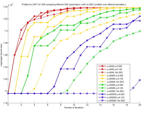
Figure 2: Applying SDM-GS-ALM to CAP-101-250 using different parameterizations for the SSC condition (or none).

The results of the Test 1 set of experiments are depicted in the plots of Figure 1 (with additional Figures 2, 3 and 4 in Appendix B). The use of different penalty parameter $\rho$ values is differentiated by the use of different plot colors. The penalties are chosen so that the smallest penalties (in red) are near optimal in terms of the resulting computational performance, while the larger penalties are known beforehand to be too large for optimal performance. For testing purposes, this is the most interesting way to choose penalty values, as smaller (than optimal) penalty values yield very little difference in Lagrangian bound between the use of different SSC parameter values. Solid line and dashed line plots depict the Lagrange bounds due to the use of a more stringent SSC parameter value $\gamma=0.5$ and a more lenient value for the SSC parameter $\gamma=0.125$, respectively. The dotted line plots depict the Lagrangian values resulting from the non-use of the SSC, so that it evaluates true no matter what. The following observations are suggested from the results of these Test 1 experiments:

1. First, the most significant differences between the varied use of SSC occur when the penalty coefficient values are large. In this setting, it seems to be the case that the use of more stringent (i.e., larger) values of the SSC parameter $\gamma$ has the effect of mitigating the destabilizing effect of having a penalty parameter $\rho$ value that is too large. This is significant because the performance of iterative Lagrangian dual solution approaches based on (or related to) proximal bundle methods is sensitive to the tuning of the $\rho$ value, and the optimal tuning of such parameters is assumed to be unknown beforehand in practical applications. For this reason, any mechanism to mitigate the effect of having an unfavorable tuning of the penalty parameter is highly desirable.

2. As is the case for the proximal bundle method, information from the SSC test can be used to dynamically fine-tune the value of the penalty parameter $\rho$. For the convergence analysis culminating in Proposition 4 to remain valid, it is expected that if $\rho$ does vary with iteration $k$, that it should stabilize to some positive value.

3. While not enforcing the SSC can adversely affect the growth trend in the Lagrangian bound, the use of a SSC parameter $\gamma$ value that is too large can have a similar effect for the tail-end values. This is most clearly seen in the Figure 1 DCAP-233-500 $\rho=50$ and $\rho=100$ plots. In these plots, the growth in Lagrangian bound value is noticeably stunted in the tail-end iterations for the larger $\gamma=0.5$ value as compared with the smaller $\gamma=0.125$.

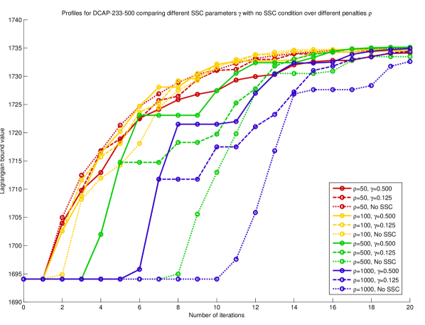
Figure 1: Applying SDM-GS-ALM using different parameterizations for the SSC condition (or none).

For the Test 2 experiments, we primarily compare the parallel speedup achieved with Algorithm 3 against that achieved with the enhancements to the proximal bundle method presented in LubinEtAl2013 . Additionally, we compare the Lagrangian bound at the final iteration.

The enhancements in LubinEtAl2013 use structure-exploiting primal-dual interior point solvers to improve the parallel efficiency of solving the proximal bundle method master problem. (The solution of this master problem is analogous to the approximated solution to problem (7) obtained by using the SDM-GS method in Algorithm 2.) The first solver is referred to by its acronym OOQP GertzWright2003 , while the second is PIPS-IPM LubinEtAl2011 .

In the experiments of Test 2, the underlying computing architecture and third-party software are inevitably different between our tests and those in LubinEtAl2013 . Additionally, the termination criterion is necessarily different from that given in Step 2 of Figure 2 in LubinEtAl2013 due to the differences in algorithms. In our tests, the termination criterion comes from Lines 9–11 of Algorithm 3 with $\epsilon=10^{-6}$. We can nevertheless create a meaningful control in the tuning of the most important parameters affecting the performance of the algorithm.

1. As done in  LubinEtAl2013 , we set the SSC parameter $\gamma=0.1$, and we initialize the dual solution $\omega^{0}=0$.

2. In analogy to the possible trimming of cutting planes noted in LubinEtAl2013 , practical implementations of Algorithm 3 may judiciously trim the set $D$ to improve performance. As all cuts are kept in the experiments of LubinEtAl2013 , so we also avoid trimming the expansion of $D$ in our experiments, and so we just use the simple update rule $D\leftarrow\operatorname{conv}(D\cup\left\{\widetilde{x},\widehat{x}\right\})$ within Algorithm 2.

3. We use an update rule analogous to the one in Kiwiel1995 as is done in LubinEtAl2013 . which takes the suggested form given in Line 17 of Algorithm 3. Initially, $\rho=1$.

In Tables 1–2, the columns headed by OOQP and PIPS-IPM report the parallel speedup due to the use of $N=1,8,16,32$ processors, which are originally reported in Figure 2 of LubinEtAl2013 . If, given the use of $N$ processors, $T_{N}$ denotes the total wall clock time (in seconds) divided by number of iterations, then we compute the parallel speedup as $T_{1}/T_{N}$. For the computational experiments with Algorithm 3, we compute each table entry $T_{1}/T_{N}$ after taking, from five identically parameterized experiments, 1) the minimum $T_{1}$ value, and 2) the average $T_{N}$, $N>1$, value. The column headed by SDM-GS1-ALM presents the parallel speedup values for the application of Algorithm 3 with $t_{max}=1$. The column headed by SDM-GS5-ALM is analogous, with $t_{max}=5$. The total wall clock time per iteration values used to compute the ratios $T_{1}/T_{N}$ are provided in Appendix C, accounting for taking the minimum ($N=1$) or average ($N>1$) over the five experiments for each set of parameterizations associated with Algorithm 3. For the two sets of experiments based on the application of Algorithm 3, a problem-specific maximum number of main loop iterations was set so as to make the tests as comparable with the tests in LubinEtAl2013 as possible. These data are also reported in Appendix C. Also in Tables 1–2, the best Lagrangian bounds obtained for each combination of test problem and algorithm are reported.

	Speedup for SSLP 5-25-100
No. Proc.	OOQP	PIPS-IPM	SDM-GS1-ALM	SDM-GS5-ALM
1	1.00	1.00	1.00	1.00
8	5.54	5.23	4.38	4.78
16	8.89	8.55	6.61	7.07
32	11.69	11.94	8.19	8.89
Lagr. Value	-127.37	-127.37	-127.71	-127.58
	Speedup for SSLP 10-50-500
No. Proc.	OOQP	PIPS-IPM	SDM-GS1-ALM	SDM-GS5-ALM
1	1.00	1.00	1.00	1.00
8	2.64	2.80	6.87	6.95
16	2.70	2.92	12.95	12.84
32	2.98	3.40	21.67	20.98
Lagr. Value	-349.14	-349.14	-349.48	-349.14
	Speedup for SSLP 10-50-2000
No. Proc.	SDM-GS1-ALM		SDM-GS5-ALM
1	1.00		1.00
2	2.34		2.34
4	4.81		4.83
8	9.29		9.25
16	18.69		18.48
32	34.63		35.10
64	60.59		60.93
Lagr. Value	-348.35		-347.75

Table 1: SSLP: Comparing speedup and final best Lagrangian bound

	Speedup for DCAP 233-500
No. Proc.	OOQP	PIPS-IPM	SDM-GS1-ALM	SDM-GS5-ALM
1	1.00	1.00	1.00	1.00
8	2.44	5.32	6.88	8.11
16	2.81	8.15	13.28	15.65
32	1.63	10.25	23.42	27.40
Lagr. Value	1736.68	1736.68	1734.99	1736.02
	Speedup for DCAP 243-500
No. Proc.	OOQP	PIPS-IPM	SDM-GS1-ALM	SDM-GS5-ALM
1	1.00	1.00	1.00	1.00
8	2.85	5.71	6.51	7.61
16	3.59	5.85	12.28	14.44
32	1.98	6.44	21.99	25.25
Lagr. Value	2165.48	2165.50	2162.58	2164.48
	Speedup for DCAP 332-500
No. Proc.	OOQP	PIPS-IPM	SDM-GS1-ALM	SDM-GS5-ALM
1	1.00	1.00	1.00	1.00
8	2.03	5.56	6.83	8.50
16	2.33	5.00	12.84	16.20
32	1.21	6.61	21.83	23.48
Lagr. Value	1587.44	1587.44	1584.77	1586.11
	Speedup for DCAP 342-500
No. Proc.	OOQP	PIPS-IPM	SDM-GS1-ALM	SDM-GS5-ALM
1	1.00	1.00	1.00	1.00
8	2.45	3.78	7.16	8.25
16	2.71	4.36	12.95	15.49
32	1.84	4.64	22.41	26.93
Lagr. Value	1902.84	1903.21	1900.81	1901.90

Table 2: DCAP: Comparing speedup and final best Lagrangian bound

We draw the following conclusions from the results of the Test 2 experiments reported in Tables 1–2.

1. The improvement in parallel speedup (SDM-GS-ALM columns) over either OOQP or PIPS-IPM is evident for all problems except for the one with the fewest number of scenarios (SSLP 5-25-100).

2. Slightly inferior final Lagrange bounds reported for SDM-GS1-ALM ($t_{max}=1$) are evident. This deficit is improved by using SDM-GS with $t_{max}=5$, as done for the SDM-GS5-ALM experiments. But even these bounds are usually not as good as the bounds obtained with OOQP or PIPS-IPM; this is due to their more exact solving of the master problem instances. This suggests that as the iterations $k\geq 1$ increase, it is advantageous to solve the continuous master problem with SDM-GS iterations using larger $t_{max}$ values.

3. Interestingly, parallel speedup is enhanced for SDM-GS5-ALM over SDM-GS1-ALM; although the latter yields lower average total wall clock time per iteration, the proportion of efficiently parallelizable work seems to increase in the former.

For Test 2, we also tested the performance of Algorithm 3 on the SSLP 10-50-2000 problem, which is of substantially larger scale than the other test problems considered in this paper. Using $N=1,2,4,8,16,32,64$ processors, we see very good speedup, which suggests the realized benefit of distributing the use of memory. We also see that for such large-scale problems, the additional cost in time of performing more inner loop Gauss-Seidel iterations (larger $t_{max}$) becomes marginal, since the cost of solving the mixed-integer linear subproblems takes a larger share of the computational time.

5 Conclusion and future work

Our contribution is motivated by the goal of improving the efficiency of parallelization applied to iterative approaches for solving the Lagrangian dual problem of large scale optimization problems. These problems have nonlinear convex differentiable objective $f$, decomposable nonconvex constraint set $X$, and nondecomposable affine constraint set $Qx=z$ to which Lagrangian relaxation is applied. Problems of such a form include the split variable extensive form of mixed-integer linear stochastic programs as a special case. Implicitly, our approach refers to the convex hull $\operatorname{conv}(X)$ of $X$, and the assumed lack of known description of $\operatorname{conv}(X)$ needs to be addressed. Proximal bundle methods (alternatively in the form of the proximal simplicial decomposition method or stabilized column generation) are well-known for addressing the latter issue. In the former issue, that of exploiting the large scale structure to apply parallel computation efficiently, we develop a modified augmented Lagrangian (AL) method with approximate subproblem solutions that incorporates ideas from the proximal bundle method.

The approximation of subproblem solutions is based on an iterative approach that integrates ideas from the simplicial decomposition method (SDM) (for constructing inner approximations of $\operatorname{conv}(X)$) and the nonlinear block Gauss-Seidel method. It is the latter Gauss-Seidel aspect that is primarily responsible for enhancing the parallel efficiency that is observed in the numerical experiments. While convergence analysis of the integrated SDM-GS approach may be derived from slight modifications to results in Bonettini2011 , for the sake of completeness and explicitness, we provide in the appendix a proof of optimal convergence of SDM-GS as it is applied within our algorithm under a standard set of conditions. A distinction between so-called “serious” steps and “null” steps, in analogy to the proximal bundle method, is also recovered. Once these aspects are successfully integrated, then the contribution is complete, where the beneficial stabilization associated with proximal point methods and the ability to apply parallelization more efficiently are both realized. The resulting algorithm developed in this paper is referred to as SDM-GS-ALM, which has similar functionality to the alternating direction method of multipliers (ADMM).

We performed numerical tests of two sorts. In Test 1, we examined the impact of varying the serious step condition parameter. We found that parameterizations that effect more stringent serious step conditions seem to have the effect of mitigating the early iteration instability due to penalty parameters that are too large. At the same time, the more stringent serious step condition parameterizations seemed to result in slower convergence to dual optimality in the tail-end. As is the case for proximal bundle methods, information obtained in the serious step condition tests may be used to beneficially adjust the proximal term penalty coefficient in early iterations.

In Test 2, we examined the efficiency of parallelization, measured by the speedup ratio, due to the use of the SDM-GS-ALM, compared versus pre-existing implementations of the proximal bundle method that use structure exploiting primal dual interior point methods to improve parallel efficiency. We saw in these results a promising increase in parallel efficiency due to the use of SDM-GS-ALM, where the increase in parallel efficiency is attributed primarily to the successful incorporation of Gauss-Seidel iterations. The results of the last problem tested, SSLP 10-50-2000, additionally suggested a benefit due to the ability of SDM-GS-ALM to distribute not just the workload, but also the use of memory. The vector of auxiliary variables $z$ is the only substantial block of data that needs to be stored and modified by all processors. In the context of stochastic optimization problems, this represents a modest communication bottleneck in proportion to the number of first-stage variables for two-stage problems, while for multistage problems, the amount of such data that must be stored by every processor and modified by parallel communication can increase exponentially with the number of stages.

Potential future improvements include the following. While a default implementation of SDM-GS-ALM would have one Gauss-Seidel iteration per SDM-GS call, the Lagrangian bounds reported from the Test 2 experiments suggest that an improved implementation would have early iterations use one Gauss-Seidel iteration per SDM-GS call, but steadily increase the number of Gauss-Seidel iterations per SDM-GS call for the later iterations. This results in better Lagrangian bounds at termination. While these extra Gauss-Seidel iterations require extra parallel communication, the additional wall clock time required becomes increasingly marginal for larger problems where the cost of solving the SDM linearized subproblems associated with expanding the inner approximation increasingly outweighs the cost associated with computing the approximate solution of the continuous master problem and any required parallel communications.

A potentially large improvement to the speed of convergence, in terms of wall clock time, would be to incorporate into the analysis the degree to which the SDM linearized subproblem can be solved suboptimally and yet retain the optimal convergence. We expect that solving these subproblems exactly, particularly in the early iterations, is highly wasteful, and providing a theoretical basis for controlling the tolerance of solution inaccuracy would be of great value. Another potential avenue for future work is to extend the experimental analysis to multistage mixed-integer stochastic optimization problems and/or nonlinear problems, as the form of the problem addressed by SDM-GS-ALM is general enough to model these types of problems.

Appendix A Technical lemmas for establishing optimal convergence of SDM-GS

Given initial $(x^{0},z^{0})\in X\times Z\subset\mathbb{R}^{n}\times\mathbb{R}^{q}$, we consider the generation of the sequence $\left\{(x^{k},z^{k})\right\}$ with iterations computed using Algorithm 4, whose target problem is given by

$$\min_{x,z}\left\{F(x,z):x\in X,z\in Z\right\},$$ (34)

where $(x,z)\mapsto F(x,z)$ is convex and continuously differentiable over $X\times Z$, and sets $X$ and $Z$ are closed and convex, with $X$ bounded and $z\mapsto F(x,z)$ is inf-compact for each $x\in X$.

We define the directional derivative with respect to $x$ as

$$F_{x}^{\prime}(x,z;d):=\lim_{\alpha\downarrow 0}\frac{F(x+\alpha d,z)-F(x,z)}{\alpha}.$$

Of interest is the satisfaction of the following local stationarity condition at $x\in X$:

$$F_{x}^{\prime}({x},{z};d)\geq 0\quad\text{for all}\;d\in X-\left\{{x}\right\}$$ (35)

for any limit point $(x,z)=(\bar{x},\bar{z})$ of some sequence $\left\{(x^{k},z^{k})\right\}$ of feasible solutions to problem (34). For the sake of nontriviality, we shall assume that the $x$-stationarity condition (35) never holds at $(x,z)=(x^{k},z^{k})$ for any $k\geq 0$. Thus, for each $x^{k}$, $k\geq 0$, there always exists a $d^{k}\in X-\left\{x^{k}\right\}$ for which $F_{x}^{\prime}(x^{k},z^{k};d^{k})<0$.

Direction Assumptions (DAs): For each iteration $k\geq 0$, given $x^{k}\in X$ and $z^{k}\in Z$, we have $d^{k}$ chosen so that 1) $x^{k}+d^{k}\in X$; and 2) $F_{x}^{\prime}(x^{k},z^{k};d^{k})<0$.

Gradient Related Assumption (GRA): Given a sequence $\left\{(x^{k},z^{k})\right\}$ with $\lim_{k\to\infty}(x^{k},z^{k})=(\overline{x},\overline{z})$, and a bounded sequence $\left\{d^{k}\right\}$ of directions, then the existence of a direction $\overline{d}\in X-\left\{\overline{x}\right\}$ such that $F_{x}^{\prime}(\overline{x},\overline{z};\overline{d})<0$ implies that

$$\limsup_{k\to\infty}F_{x}^{\prime}(x^{k},z^{k};d^{k})<0.$$ (36)

In this case, we say that $\left\{d^{k}\right\}$ is gradient related to $\left\{x^{k}\right\}$. This gradient related condition is similar to the one defined in Bertsekas1999 . The sequence of directions ${d^{k}}$ is typically gradient related to $\left\{x^{k}\right\}$ by construction. (See Lemma 7.)

To state the last assumption, we require the notion of an Armijo rule step length $\alpha^{k}\in(0,1]$ given $(x^{k},z^{k},d^{k})$ and parameters $\beta,\sigma\in(0,1)$.

Algorithm 4 Computing an Armijo rule step length $\alpha^{k}$ at iteration $k$.

1:function ArmijoStep($F$, $x^{k}$, $z^{k}$, $d^{k}$, $\beta$, $\sigma$)

2:     $\alpha^{k}\leftarrow 1$

3:     while $F(x^{k}+\alpha^{k}d^{k},z^{k})-F(x^{k},z^{k})>\alpha^{k}\sigma F_{x}^{\prime}(x^{k},z^{k};d^{k})$ do

4:         $\alpha^{k}\leftarrow\beta\alpha^{k}$

5:     end while

6:     return $\alpha^{k}$

7:end function

Remark 6

Under mild assumptions on $F$ such as continuity that guarantee the existence of finite $F_{x}^{\prime}(x,z;d)$ for all $(x,z,d)\in\left\{(x,z,d):x\in X,d\in X-\left\{x\right\},z\in Z\right\}$, we may assume that the while loop of Lines 3–5 terminates after a finite number of iterations. Thus, we have $\alpha^{k}\in(0,1]$ for each $k\geq 1$.

The last significant assumption is stated as follows.

Sufficient Decrease Assumption (SDA): For sequences $\left\{(x^{k},z^{k},d^{k})\right\}$ and step lengths $\left\{\alpha^{k}\right\}$ computed according to Algorithm 4, we assume for each $k\geq 0$, that $(x^{k+1},z^{k+1})$ satisfies

$$F(x^{k+1},z^{k+1})\leq F(x^{k}+\alpha^{k}d^{k},z^{k}).$$

Lemma 6

For problem (34), let $F:\mathbb{R}^{n_{x}}\times\mathbb{R}^{n_{z}}\mapsto\mathbb{R}$ be convex and continuously differentiable, $X\subset\mathbb{R}^{n_{x}}$ convex and compact, and $Z\subseteq\mathbb{R}^{n_{z}}$ closed and convex. Furthermore, assume for each $x\in X$ that $z\mapsto F(x,z)$ is inf-compact. If a sequence $\left\{(x^{k},z^{k},d^{k})\right\}$ satisfies the DA, the GRA, and the SDA for some fixed $\beta,\sigma\in(0,1)$, then the sequence ${(x^{k},z^{k})}$ has limit points $(\overline{x},\overline{z})$, each of which satisfies the stationarity condition (35).

Proof

The existence of limit points $(\overline{x},\overline{z})$ follows from the compactness of $X$, the inf-compactness of $z\mapsto F(x,z)$ for each $x\in X$, and the SDA.

In generating $\left\{\alpha^{k}\right\}$ according to the Armijo rule as implemented in Lines 2–5 of Algorithm 4, we have

$$\frac{F(x^{k}+\alpha^{k}d^{k},z^{k})-F(x^{k},z^{k})}{\alpha^{k}}\leq\sigma F_{x}^{\prime}(x^{k},z^{k};d^{k}).$$ (37)

By the DA, $F_{x}^{\prime}(x^{k},z^{k};d^{k})<0$ and since $\alpha^{k}>0$ for each $k\geq 1$ by Remark 6, we infer from (37) that $F(x^{k}+\alpha^{k}d^{k},z^{k})<F(x^{k},z^{k}).$ By construction, we have $F(x^{k+1},z^{k+1})\leq F(x^{k}+\alpha^{k}d^{k},z^{k})<F(x^{k},z^{k}).$ By the monotonicity $F(x^{k+1},z^{k+1})<F(x^{k},z^{k})$ and $F$ being bounded from below on $X\times Z$, we have $\lim_{k\to\infty}F(x^{k},z^{k})=\bar{F}>-\infty$. Therefore,

$$\lim_{k\to\infty}F(x^{k+1},z^{k+1})-F(x^{k},z^{k})=0,$$

which implies

$$\lim_{k\to\infty}F(x^{k}+\alpha^{k}d^{k},z^{k})-F(x^{k},z^{k})=0.$$ (38)

We assume for sake of contradiction that $\lim_{k\to\infty}(x^{k},z^{k})=(\overline{x},\overline{y})$ does not satisfy the stationarity condition (35). By GRA, we have that $\left\{d^{k}\right\}$ is gradient related to $\left\{x^{k}\right\}$; that is,

$$\limsup_{k\to\infty}F_{x}^{\prime}(x^{k},z^{k};d^{k})<0.$$ (39)

Thus, it follows from (37)–(39) that $\lim_{k\to\infty}\alpha^{k}=0$.

Consequently, after a certain iteration $k\geq\bar{k}$, we can define $\left\{\bar{\alpha}^{k}\right\}$, $\bar{\alpha}^{k}=\alpha^{k}/\beta$, where $\bar{\alpha}^{k}\leq 1$ for $k\geq\bar{k}$, and so we have

$$\sigma F_{x}^{\prime}(x^{k},z^{k};d^{k})<\frac{F(x^{k}+\bar{\alpha}^{k}d^{k},z^{k})-F(x^{k},z^{k})}{\bar{\alpha}^{k}}.$$ (40)

Since $F$ is continuously differentiable, the mean value theorem may be applied to the right-hand side of (40) to get

$$\sigma F_{x}^{\prime}(x^{k},z^{k};d^{k})<F_{x}^{\prime}(x^{k}+\widetilde{\alpha}^{k}d^{k},z^{k};d^{k}),$$ (41)

for some $\widetilde{\alpha}^{k}\in[0,\overline{\alpha}^{k}]$.

Again, using the assumption $\limsup_{k\to\infty}F_{x}^{\prime}(x^{k},z^{k};d^{k})<0$, and also the compactness of $X-X$, we take a limit point $\overline{d}$ of $\left\{d^{k}\right\}$, with its associated subsequence index set denoted by $\mathcal{K}$, such that $F_{x}^{\prime}(\overline{x},\overline{z},\overline{d})<0$. Taking the limits over the subsequence indexed by $\mathcal{K}$, we have $\lim_{k\to\infty,k\in\mathcal{K}}F_{x}^{\prime}(x^{k},z^{k};d^{k})=F_{x}^{\prime}(\overline{x},\overline{z};\overline{d})$ and $\lim_{k\to\infty,k\in\mathcal{K}}F_{x}^{\prime}(x^{k}+\widetilde{\alpha}^{k}d^{k},z^{k};d^{k})=F_{x}^{\prime}(\overline{x},\overline{z};\overline{d})$. These two limits holds since 1) $(x,z)\mapsto F_{x}^{\prime}(x,z;d)$ for each $d\in X-X$ is continuous and 2) $d\mapsto F_{x}^{\prime}(x,z;d)$ is locally Lipschitz continuous for each $(x,z)\in X\times Z$ (e.g., Proposition 2.1.1 of Clarke1990 ); these two facts together imply that $(x,z;d)\mapsto F_{x}^{\prime}(x,z;d)$ is continuous. Then, inequality (41) becomes in the limit as $k\to\infty$, $k\in\mathcal{K}$,

$$\sigma F_{x}^{\prime}(\overline{x},\overline{z};\overline{d})\leq F_{x}^{\prime}(\overline{x},\overline{z};\overline{d}),$$

$$\Longrightarrow\quad 0\leq(1-\sigma)F_{x}^{\prime}(\overline{x},\overline{z};\overline{d}).$$

Since $(1-\sigma)>0$ and $F_{x}^{\prime}(\overline{x},\overline{z};\overline{d})<0$, we have a contradiction. Thus, $\overline{x}$ must satisfy the stationary condition (35).

Remark 7

Noting that $F_{x}^{\prime}(x^{k},z^{k};d^{k})=\nabla_{x}F(x^{k},z^{k})d^{k}$ under the assumption of continuous differentiability of $F$, one means of constructing $\left\{d^{k}\right\}$ is as follows:

$$d^{k}\leftarrow\operatorname*{argmin}_{d}\left\{\nabla_{x}F(x^{k},z^{k})d:d\in X-\left\{x^{k}\right\}\right\}.$$ (42)

Lemma 7

Given sequence $\left\{(x^{k},z^{k})\right\}$ with $\lim_{k\to\infty}(x^{k},z^{k})=(\overline{x},\overline{z})$, let each $d^{k}$, $k\geq 1$, be generated as in (42). Then $\left\{d^{k}\right\}$ is gradient related to $\left\{x^{k}\right\}$.

Proof

By the construction of $d^{k}$, $k\geq 1$, we have

$$F_{x}^{\prime}(x^{k},z^{k};d^{k})\leq F_{x}^{\prime}(x^{k},z^{k};d)\quad\forall\;d\in X-\left\{x^{k}\right\}.$$

Taking the limit, we have

$$\limsup_{k\to\infty}F_{x}^{\prime}(x^{k},z^{k};d^{k})\leq\limsup_{k\to\infty}F_{x}^{\prime}(x^{k},z^{k};d)\leq F_{x}^{\prime}(\overline{x},\overline{z};d)\quad\forall\;d\in X-\left\{\overline{x}\right\},$$

where the last inequality follows from the upper semicontinuity of the function $(x,z,d)\mapsto F_{x}^{\prime}(x,z;d)$, which holds in our setting due, primarily, to Proposition 2.1.1 (b) of  Clarke1990 given that $F$ is assumed to be convex and continuous on $\mathbb{R}^{n}$. Taking $\overline{d}\in\operatorname*{argmin}_{d}\left\{F_{x}^{\prime}(\overline{x},\overline{z};d):d\in X-\left\{\overline{x}\right\}\right\}$, we have by the assumed nonstationarity that $F_{x}^{\prime}(\overline{x},\overline{z};\overline{d})<0$. Thus, $\limsup_{k\to\infty}F_{x}^{\prime}(x^{k},z^{k};d^{k})<0,$ and so GRA holds.

Appendix B Supplementary Material: Additional Figures

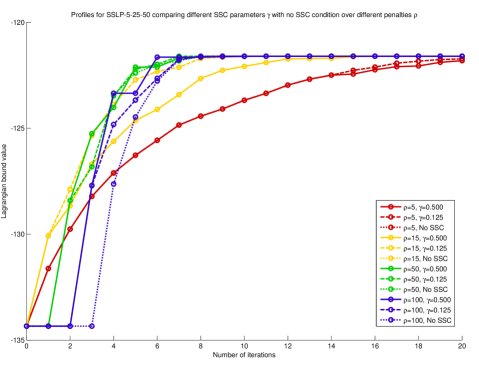
Figure 3: Applying SDM-GS-ALM to SSLP-5-25-50 using different parameterizations for the SSC condition (or none).

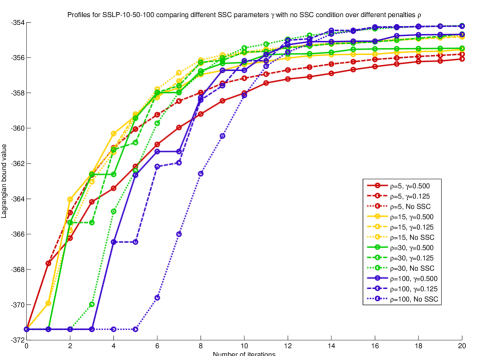
Figure 4: Applying SDM-GS-ALM to SSLP-10-50-100 using different parameterizations for the SSC condition (or none).

Appendix C Supplementary Material: Additional Tables

For each entry $(A,B)$ of Tables 3 and 4, $A$ provides the number of iterations at termination, and $B$ provides the average wall clock time (in seconds) per iteration.

	SSLP 5-25-100
No. Proc.	OOQP	PIPS-IPM	SDM-GS1-ALM	SDM-GS5-ALM
1	(8, 6.31)	(8, 6.33)	(8,3.22)	(8,3.32)
8	(8, 1.14)	(8, 1.21)	(8,0.74)	(8,0.69)
16	(8, 0.71)	(8, 0.74)	(8,0.49)	(8,0.47)
32	(8, 0.54)	(8, 0.53)	(8,0.39)	(8,0.37)
	SSLP 10-50-500
No. Proc.	OOQP	PIPS-IPM	SDM-GS1-ALM	SDM-GS5-ALM
1	(26, 3301)	(22, 2939)	(30, 168.80)	(29, 171.85)
8	(31, 1252)	(24, 1049)	(30, 24.58)	(29, 24.71)
16	(27, 1224)	(28, 1005)	(30, 13.04)	(30, 13.39)
32	(31, 1106)	(27, 865)	(30, 7.79)	(28, 8.19)
	SSLP 10-50-2000
No. Proc.	SDM-GS1-ALM		SDM-GS5-ALM
1	(20, 840.69)		(20, 845.77)
2	(20, 359.63)		(20, 361.40)
4	(20, 174.83)		(20, 175.03)
8	(20, 90.51)		(20, 91.46)
16	(20, 44.98)		(20, 45.76)
32	(20, 24.27)		(20, 24.09)
64	(20, 13.87)		(20, 13.88)

Table 3: SSLP: Reporting auxiliary data

	DCAP 233-500
No. Proc.	OOQP	PIPS-IPM	SDM-GS1-ALM	SDM-GS5-ALM
1	(68, 16.15)	(66, 12.71)	(68, 3.67)	(68, 5.21)
8	(68, 6.62)	(70, 2.39)	(68, 0.53)	(68, 0.64)
16	(68, 5.75)	(73, 1.56)	(68, 0.28)	(68, 0.33)
32	(68, 9.91)	(70, 1.24)	(68, 0.16)	(68, 0.19)
	DCAP 243-500
No. Proc.	OOQP	PIPS-IPM	SDM-GS1-ALM	SDM-GS5-ALM
1	(57, 14.37)	(57, 12.11)	(57, 3.72)	(57, 5.11)
8	(57, 5.04)	(58, 2.12)	(57, 0.57)	(57, 0.67)
16	(57, 4.00)	(59, 2.07)	(57, 0.30)	(57, 0.35)
32	(57, 7.26)	(59, 1.88)	(57, 0.17)	(57, 0.20)
	DCAP 332-500
No. Proc.	OOQP	PIPS-IPM	SDM-GS1-ALM	SDM-GS5-ALM
1	(82, 13.51)	(80, 9.45)	(82, 2.94)	(82, 4.85)
8	(82, 6.65)	(79, 1.70)	(81, 0.43)	(82, 0.57)
16	(82, 5.81)	(80, 1.89)	(81, 0.23)	(82, 0.30)
32	(82, 11.20)	(77, 1.43)	(82, 0.13)	(82, 0.21)
	DCAP 342-500
No. Proc.	OOQP	PIPS-IPM	SDM-GS1-ALM	SDM-GS5-ALM
1	(59, 14.78)	(71, 12.07)	(59, 3.80)	(59, 5.57)
8	(59, 6.03)	(67, 3.19)	(59, 0.53)	(59, 0.68)
16	(59, 5.46)	(56, 2.77)	(59, 0.29)	(59, 0.36)
32	(59, 8.05)	(62, 2.60)	(59, 0.17)	(59, 0.21)

Table 4: DCAP: Reporting auxiliary data

References

- (1) COmputational INfrastructure for Operations Research. URL http://www.coin-or.org/. Last accessed 28 January, 2016
- (2) Ahmed, S., Garcia, R., Kong, N., Ntaimo, L., Parija, G., Qiu, F., Sen, S.: SIPLIB: A stochastic integer programming test problem library (2015). URL http://www.isye.gatech.edu/ sahmed/siplib
- (3) Amor, H.B., Desrosiers, J., Frangioni, A.: On the choice of explicit stabilizing terms in column generation. Discrete Applied Mathematics 157(6), 1167 – 1184 (2009)
- (4) Bertsekas, D.: Constrained Optimization and Lagrange Multiplier Methods. Academic Press (1982)
- (5) Bertsekas, D.: Nonlinear Programming. Athena Scientific (1999)
- (6) Bertsekas, D.: Convex Optimization Algorithms. Athena Scientific (2015)
- (7) Bertsekas, D.: Incremental aggregated proximal and augmented Lagrangian algorithms. arXiv preprint arXiv:1509.09257 (2015)
- (8) Birge, J.R., Louveaux, F.: Introduction to Stochastic Programming. Springer Science & Business Media (2011)
- (9) Bodur, M., Dash, S., Günlük, O., Luedtke, J.: Strengthened Benders cuts for stochastic integer programs with continuous recourse (2014). URL http://www.optimization-online.org/DB_FILE/2014/03/4263.pdf. Last accessed on 13 January 2015
- (10) Boland, N., Christiansen, J., Dandurand, B., Eberhard, A., Linderoth, J., Luedtke, J., Oliveira, F.: Progressive hedging with a Frank-Wolfe based method for computing stochastic mixed-integer programming Lagrangian dual bounds. Optimization Online (2016). URL http://www.optimization-online.org/DB_HTML/2016/03/5391.html
- (11) Bonettini, S.: Inexact block coordinate descent methods with application to non-negative matrix factorization. IMA Journal of Numerical Analysis 31(4), 1431–1452 (2011)
- (12) Boyd, S., Parikh, N., Chu, E., Peleato, B., Eckstein, J.: Distributed optimization and statistical learning via the alternating direction method of multipliers. Foundation and Trends in Machine Learning 3(1), 1–122 (2011)
- (13) Carøe, C.C., Schultz, R.: Dual decomposition in stochastic integer programming. Operations Research Letters 24(1), 37–45 (1999)
- (14) Chatzipanagiotis, N., Dentcheva, D., Zavlanos, M.: An augmented Lagrangian method for distributed optimization. Mathematical Programming 152(1), 405–434 (2014)
- (15) Chen, G., Teboulle, M.: A proximal-based decomposition method for convex minimization problems. Mathematical Programming 64, 81–101 (1994)
- (16) Clarke, F.: Optimization and Nonsmooth Analysis. Society for Industrial and Applied Mathematics (1990)
- (17) Eckstein, J.: A practical general approximation criterion for methods of multipliers based on Bregman distances. Mathematical Programming 96(1), 61–86
- (18) Eckstein, J., Bertsekas, D.: On the Douglas-Rachford splitting method and the proximal point algorithm for maximal monotone operators. Mathematical Programming 55(1-3), 293–318 (1992)
- (19) Eckstein, J., Silva, P.: A practical relative error criterion for augmented lagrangians. Mathematical Programming 141(1), 319–348 (2013)
- (20) Eckstein, J., Yao, W.: Understanding the convergence of the alternating direction method of multipliers: Theoretical and computational perspectives. Tech. rep., Rutgers University (2014)
- (21) Feizollahi, M.J., Costley, M., Ahmed, S., Grijalva, S.: Large-scale decentralized unit commitment. International Journal of Electrical Power & Energy Systems 73, 97–106 (2015)
- (22) Fischer, F., Helmberg, C.: A parallel bundle framework for asynchronous subspace optimization of nonsmooth convex functions. SIAM Journal on Optimization 24(2), 795–822 (2014)
- (23) Gabay, D., Mercier, B.: A dual algorithm for the solution of nonlinear variational problems via finite element approximation. Computers and Mathematics with Applications 2, 17–40 (1976)
- (24) Gade, D., Hackebeil, G., Ryan, S.M., Watson, J.P., Wets, R.J.B., Woodruff, D.L.: Obtaining lower bounds from the progressive hedging algorithm for stochastic mixed-integer programs. Mathematical Programming 157(1), 47–67 (2016)
- (25) Gertz, E., Wright, S.: Object-oriented software for quadratic programming. ACM Transactions on Mathematical Software 29(1), 58–81 (2003)
- (26) Glowinski, R., Marrocco, A.: Sur l’approximation, par elements finis d’ordre un, et la resolution, par penalisation-dualité, d’une classe de problems de dirichlet non lineares. Revue Française d’Automatique, Informatique, et Recherche Opérationelle 9, 41–76 (1975)
- (27) Grippo, L., Sciandrone, M.: On the convergence of the block nonlinear Gauss-Seidel method under convex constraints. Operations Research Letters 26(3), 127–136 (2000)
- (28) Hamdi, A., Mahey, P., Dussault, J.P.: Recent Advances in Optimization: Proceedings of the 8th French-German Conference on Optimization Trier, July 21–26, 1996, chap. A New Decomposition Method in Nonconvex Programming via a Separable Augmented Lagrangian, pp. 90–104. Springer Berlin Heidelberg, Berlin, Heidelberg (1997)
- (29) Hare W., S.C.S.M.: A proximal bundle method for nonsmooth nonconvex functions with inexact information. Computational Optimization and Applications 63, 1–28 (2016)
- (30) Hathaway, R.J., Bezdek, J.C.: Grouped coordinate minimization using Newton’s method for inexact minimization in one vector coordinate. Journal of Optimization Theory and Applications 71(3), 503–516 (1991)
- (31) He, B., Liao, L.Z., Han, D., Yang, H.: A new inexact alternating directions method for monotone variational inequalities. Mathematical Programming 92, 103–118 (2002)
- (32) Hestenes, M.R.: Multiplier and gradient methods. Journal of Optimization Theory and Applications pp. 303–320 (1969)
- (33) Hildreth, C.: A quadratic programming procedure. Naval Research Logistics Quarterly 4, 79–85, 361 (1957)
- (34) Holloway, C.: An extension of the Frank and Wolfe method of feasible directions. Mathematical Programming 6(1), 14–27 (1974)
-
(35)
IBM Corporation: IBM ILOG CPLEX Optimization Studio CPLEX User’s Manual.
URL http://www.ibm.com/support/knowledgecenter/en/SSSA5P_12.6.1/
ilog.odms.studio.help/pdf/usrcplex.pdf. Last accessed 22 August 2016 - (36) IBM Corporation: IBM ILOG CPLEX V12.5. URL http://www-01.ibm.com/software/commerce/optimization/cplex-optimizer/. Last accessed 28 Jan 2016
- (37) Kiwiel, K., Rosa, C., Ruszczyński, A.: Proximal decomposition via alternating linearization. SIAM Journal on Optimization 9(3), 668–689 (1999)
- (38) Kiwiel, K.C.: Approximations in proximal bundle methods and decomposition of convex programs. Journal of Optimization Theory and Applications 84(3), 529–548 (1995)
- (39) Lemaréchal, C.: An extension of Davidon methods to non differentiable problems, pp. 95–109. Springer Berlin Heidelberg (1975)
- (40) Lin, X., Pham, M., Ruszczyński, A.: Alternating linearization for structured regularization problems. Journal of Machine Learning Research 15, 3447–3481 (2014)
- (41) Lubin, M., Martin, K., Petra, C., Sandıkçı, B.: On parallelizing dual decomposition in stochastic integer programming. Operations Research Letters 41(3), 252–258 (2013)
- (42) Lubin, M., Petra, C., Anitescu, M., Zavala, V.: Scalable stochastic optimization of complex energy systems. In: Proceedings of 2011 International Conference for High Performance Computing, Networking, Storage and Analysis, p. 64:1–64:10. ACM, Seattle, WA (2011)
- (43) Mahey, P., Oualibouch, S., Tao, P.D.: Proximal decomposition on the graph of a maximal monotone operator. SIAM Journal on Optimization 5(2), 454–466 (1995)
- (44) The MathWorks, Natick: MATLAB 2012b (2014)
- (45) Mulvey, J., Ruszczyński, A.: A diagonal quadratic approximation method for large scale linear programs. Operations Research Letters 12(4), 205 – 215 (1992)
- (46) National Computing Infrastructure (NCI): NCI Website. URL http://www.nci.org.au. Last accessed 19 November 2016
- (47) Ntaimo, L.: Decomposition algorithms for stochastic combinatorial optimization: Computational experiments and extensions. Ph.D. thesis (2004)
- (48) de Oliveira, W., Sagastizábal, C.: Bundle Methods in the XXIst Century: A Bird’s-eye view. Pesquisa Operacional 34, 647–670 (2014)
- (49) de Oliveira, W., Sagastizábal, C., Lemaréchal, C.: Convex proximal bundle methods in depth: a unified analysis for inexact oracles. Mathematical Programming 148(1), 241–277 (2014)
- (50) Powell, M.J.D.: A method for nonlinear constraints in minimization problems. In: R. Fletcher (ed.) Optimization. New York: Academic Press (1969)
- (51) Rockafellar, R.: Convex Analysis. Princeton University Press (1970)
- (52) Rockafellar, R.: Monotone operators and the proximal point algorithm. SIAM Journal on Control and Optimization 14(5), 877–898 (1976)
- (53) Rockafellar, R.T.: Augmented Lagrangians and applications of the proximal point algorithm in convex programming. Mathematics of Operations Research 1(2), 97–116 (1976)
- (54) Ruszczyński, A.: Nonlinear Optimization. Princeton University Press (2006)
- (55) Ruszczyński, A.: On convergence of an augmented Lagrangian decomposition method for sparse convex optimization. Mathematics of Operations Research 20(3), 634–656 (1995)
- (56) Shor, N.: Minimization Methods for Non-differentiable Functions. Springer-Verlag, New York (1985)
- (57) Tappenden, R., Richtárik, P., Büke, B.: Separable approximations and decomposition methods for the augmented Lagrangian. Optimization Methods & Software 30(3), 643–668 (2015)
- (58) Tseng, P.: Convergence of a block coordinate descent method for nondifferentiable minimization. Journal of Optimization Theory and Applications 109, 475–494 (2001)
- (59) Von Hohenbalken, B.: Simplicial decomposition in nonlinear programming algorithms. Mathematical Programming 13(1), 49–68 (1977)
- (60) Warga, J.: Minimizing certain convex functions. SIAM Journal on Applied Mathematics 11, 588–593 (1963)