Discrete Cycloids from Convex Symmetric Polygons

Abstract

Cycloids, hipocycloids and epicycloids have an often forgotten common property: they are homothetic to their evolutes. But what if use convex symmetric polygons as unit balls, can we define evolutes and cycloids which are genuinely discrete? Indeed, we can! We define discrete cycloids as eigenvectors of a discrete double evolute transform which can be seen as a linear operator on a vector space we call curvature radius space. We are also able to classify such cycloids according to the eigenvalues of that transform, and show that the number of cusps of each cycloid is well determined by the ordering of those eigenvalues. As an elegant application, we easily establish a version of the four-vertex theorem for closed convex polygons. The whole theory is developed using only linear algebra, and concrete examples are given.

1 Introduction

Euclidean cycloids (and hypocycloids and epicycloids) can be characterized as planar curves which are $\lambda-$homothetic to their evolutes (which kind of cycloid depends on the signal of $\lambda-1$). Such idea can naturally be extended to normed planes (see Cycloids ) if the unit ball is sufficiently smooth. But what if the ball is a polygon? Can we define genuinely discrete analogues of cycloids without using limiting processes?

In this paper, we present a discrete evolute transform and then define discrete cycloids as polygonal lines which are homothetic to their double evolutes. Our evolute construction is an alternative to Arnold – we follow instead the approach in Evolutes . By using a suitable representation, we can represent our polygonal lines as vectors in a space we call $L_{P}$. In this space, the double evolute transform is linear, so we rephrase the problem in two different ways: as an eigenvector problem, or as a recurrence. By analysing the interaction of this transform within many subspaces of $L_{P}$, we are able to establish the spectral representation of the double evolute transform. As a consequence, we are able to decompose any element of $L_{P}$ as a sum of cycloids, producing a generalization of the Discrete Fourier Transform. As an application of this decomposition, we provide an elegant proof of a four vertex theorem for polygons.

We provide explicit cycloid formulae when the polygon is regular; as expected, if the polygon is close to the usual euclidean unit ball, the corresponding cycloids are approximations of the classical cycloids.

More specifically, we start with a symmetric polygon $P=P_{1}P_{2}...P_{2n}$ which will be our unit ball on the plane, and define its dual ball $Q=Q_{1}Q_{2}...Q_{2n}$. A polygonal line $M$ whose sides are respectively parallel to the sides of $P$ can then be represented by the lengths $r_{1},r_{2},...$ of its sides (taking the sides of $P$ as unit length in each direction) – we call this the curvature radius representation of $M$. We show that $M$ is a cycloid exactly when its radii satisfy a difference equation of the kind

$$\frac{-1}{\left[P_{i},P_{i+1}\right]}\nabla_{i}\left(\frac{\Delta_{i}r}{\left[Q_{i},Q_{i+1}\right]}\right)=\lambda r_{i}$$ (1)

where $\Delta_{i}$ and $\nabla_{i}$ are forward and backward difference operators, and $\left[\cdot,\cdot\right]$ is the determinant of two vectors. This equation is the natural discretization of the 2nd order Sturm-Liouville type Differential Equation displayed in Cycloids , so we can reasonably expect it to have a nice spectral structure (as seen in WangShi ). Indeed, if we require the list $r_{i}$ to be $2n$-periodic, we are able to show that the eigenvalues associated to Eq. (1) can be ordered as

$$\lambda_{0}(=0)<\lambda_{1}^{1}=\lambda_{1}^{2}(=1)<\lambda_{2}^{1}\leq\lambda_{2}^{2}<\lambda_{3}^{1}\leq\lambda_{3}^{2}<...\lambda_{n-1}^{1}\leq\lambda_{n-1}^{2}<\lambda_{n}$$

where each eigenvector is a closed cycloid – except for those with eigenvalue $1$, which form a $2$-dimensional space of non-closed cycloids (there are no non-trivial hypocycloids). Moreover, we show that the cycloid associated to $\lambda_{k}^{i}$ has exactly $2k$ ordinary cusps. When $k$ is even, the cycloid is a symmetric polygon; when $k$ is odd ($\neq 1$), the cycloid is a polygon of $0$-width. It is interesting to note that, in the Euclidean case, the eigenvalue $\lambda$ is determined by the number of cusps of the cycloids – not the case here, since we might have $\lambda_{k}^{1}\neq\lambda_{k}^{2}$!

Figure 1 shows a concrete example, where the unit ball is the octagon in the top image (and the cycloid for $\lambda_{0}=0$). The next row pictures two different open cycloids ($\lambda=1$). The third row shows symmetric cycloids ($\lambda_{2}^{1}\approx 3.21$ and $\lambda_{2}^{2}\approx 3.46$), each with $4$ cusps. The fourth row shows $0$-width cycloids ($\lambda_{3}^{1}\approx 4.90$ and $\lambda_{3}^{2}\approx 7.92$), with $3$ ”double” cusps each. Finally, we have one last cycloid ($\lambda_{4}\approx 8.15$) where all $8$ vertices are cusps.

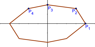
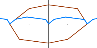
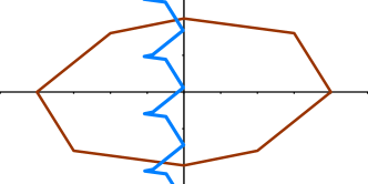
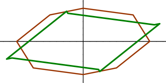
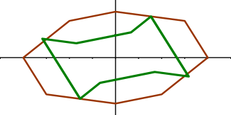
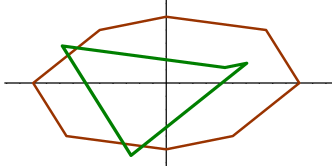
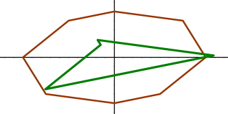
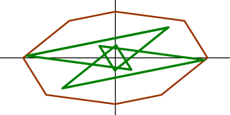
Figure 1: Cycloids related to an octagon

If we require instead the list $r_{i}$ to be just $2mn$-periodic, the old eigenvalues are joined by new ones in a very orderly fashion

$$\lambda_{0}\left(=0\right)$$

  

(note the previous eigenvalue list in the last column – they do not necessarily come in identical pairs). In summary, we have $2m-2$ non-trivial hypocycloids, $2$ cycloids and $2mn-2m-1$ epicycloids. The fractional indices work across different periods – for example, the eigenvalue $\lambda_{2/5}^{1}$ which appears when looking for a list of period $10n$ is indeed the same as $\lambda_{6/15}^{1}$ which would show up when looking for period $30n$.

Many of the results we present have been previously established in a more general context – see WangShi , for example – but our approach is very geometric and requires only basic Linear Algebra.

The organization of the paper is as follows: in section 2 we establish basic facts about the polygonal unit ball and its dual. Section 3 presents the curvature radius space (with an inner product) and establishes geometric interpretations of many of its interesting subspaces. In section 4 we present the discrete evolute and the double evolute transforms. Section 5 finally defines the cycloids, starting out with the important example when the ball is a regular polygon, and proceeds to the spectral analysis of the double evolute transform and the determination of the number of cusps of each cycloid (in the case where the cycloids have the same period as the unit ball). In section 6, we show that the general case where our cycloids have other periods than the unit ball can be reduced to the $2n$-periodic polygons, establishing the more general result. Finally, in section 7 we use our framework to quickly prove a four vertex theorem for polygons.

1.1 Notation

Given two points or vectors $v,w\in\mathbb{R}^{2}$, we denote the determinant whose columns are $v$ and $w$ by $\left[v,w\right]$. Given a list of numbers (or vectors) $\left\{L_{i}\right\}_{i\in\mathbb{Z}}$, we define the forward difference operator $\Delta L=\left\{\Delta_{i}L\right\}_{i\in\mathbb{Z}}$ where $\Delta_{i}L=L_{i+1}-L_{i}$ and the backward difference operator $\nabla L=\left\{\nabla_{i}L\right\}_{i\in\mathbb{Z}}$ where $\nabla_{i}=\Delta_{i-1}$ (whenever necessary, indices are taken mod $2n$); their composition will be denoted $\delta^{2}$ (so $\delta^{2}L=L_{i+1}-2L_{i}+L_{i-1}$). Whenever two matrices $A$ and $B$ are similar (that is, $A=M^{-1}BM$ for some invertible matrix $M$), we write $A\approx B$.

2 The polygonal ball and its dual

We start out with a plane symmetric non-degenerate convex polygon $P=P_{1}P_{2}...P_{2n}$ (that is, $P_{i+n}=-P_{i}$), which will be our reference ball of radius 1 – we might as well imagine that the vertices are in counter-clockwise order around the origin. Its dual is the only polygon $Q=Q_{1}Q_{2}...Q_{2n}$ which satisfies

$$\left[P_{i},Q_{i}\right]=1\text{ and }\left[\Delta_{i}P,Q_{i}\right]=\left[P_{i+1},\Delta_{i}Q\right]=0$$

for $i=1,...,2n$. Note that, in view of the first equation, the two last ones are actually equivalent, since

$$\Delta_{i}\left[P_{i},Q_{i}\right]=\left[\Delta_{i}P,Q_{i}\right]+\left[P_{i+1},\Delta_{i}Q\right]=0\text{.}$$

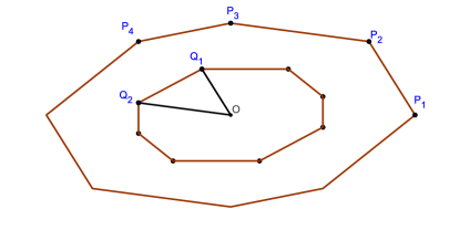
Figure 2: A $P$-ball and its dual

Geometrically, each vector $Q_{i}$ is parallel to the corresponding side of $P$, and vice-versa. These conditions actually allow us to write explicitly

$$P_{i+1}=-\alpha_{i}\Delta_{i}Q\text{ and }Q_{i}=\beta_{i}\Delta_{i}P$$ (2)

where

$$\alpha_{i}=\frac{1}{\left[Q_{i},Q_{i+1}\right]}\text{ and }\beta_{i}=\frac{1}{\left[P_{i},P_{i+1}\right]}$$ (3)

From there, it is easy to see that the dual ball is also symmetric. Moreover, since

$$\left[Q_{i-1},Q_{i}\right] =\beta_{i-1}\beta_{i}\left[\nabla_{i}P,\Delta_{i}P\right]>0$$ (4)

$$\left[\nabla_{i}Q,\Delta_{i}Q\right] =\left[\left[Q_{i-1},Q_{i}\right]P_{i},\left[Q_{i},Q_{i+1}\right]P_{i+1}\right]=\beta_{i-1}\beta_{i}\beta_{i+1}\left[\nabla_{i}P,\Delta_{i}P\right]\left[\Delta_{i}P,\Delta_{i+1}P\right]>0$$

we see that $Q$ is also convex and ordered in a counter-clockwise orientation (in particular, all $\alpha_{i}$ and $\beta_{i}$ are positive). Finally, we note for future reference that any scaling of a factor $\gamma$ applied to $P$ implies in a scaling of factor $\frac{1}{\gamma}$ applied to $Q$.

3 The curvature radius space

Consider all polygonal lines $M=\left(M_{i}\right)_{i\in\mathbb{Z}}$ whose sides are respectively parallel to the corresponding sides of $P$ (though they do not necessarily close, let us call them $P$-polygons anyway). More explicitly, we will require

$$\Delta_{i}M=r_{i}\cdot\Delta_{i}P$$

for some list of real numbers $\left(r_{i}\right)_{i\in\mathbb{Z}}$ (we allow $r_{i}=0$ with no further ado). Each number $r_{i}$ will be called the curvature radius of the side $M_{i}M_{i+1}$ (with respect to $P$). Up to a translation, all $P$-polygons are uniquely represented by the list $\left(r_{i}\right)$.

Before continuing, we add another restriction – we require the sides (but not necessarily the vertices!) to repeat:

Definition 1

A polygonal line $M$ is a periodic $P$-polygon when

$$\Delta_{i+2n}M=\Delta_{i}M$$

for all $i\in\mathbb{Z}$. Since in this case we clearly have

$$r_{i+2n}=r_{i}$$ (5)

each such polygonal line $M$ (up to a translation) can be represented by its radii vector $\vec{r}=\left(r_{i}\right)_{i=1,2,...,2n}$. We write $L_{P}$ for such space of all periodic $P$-polygons.

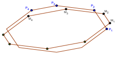
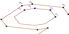
Figure 3: While $\vec{r}=\left(\frac{1}{2},1,\frac{3}{2},1,\frac{1}{2},1,\frac{3}{2},1\right)$ closes the line, $\vec{r}=\left(1,2,1,2,1,2,1,-1\right)$ does not

Our goal in this section is to pair up algebraic properties of $\vec{r}\in\mathbb{R}^{2n}$ with geometric properties of $M$ (compare this to the similar analysis done in Evolutes ). We start defining a suitable inner product in $L_{P}$:

Definition 2

Given two radii vectors $\vec{r}$ and $\vec{s}$ in $L_{P}$, we define their $P$-inner product as

$$\left\langle\vec{r},\vec{s}\right\rangle_{P}=\sum_{i=1}^{2n}\frac{r_{i}s_{i}}{\beta_{i}}$$

Some interesting subspaces of $L_{P}$ are listed below:

• $C_{P}:$ the space of all closed polygons $M.$ Given our periodicity condition on the sides, it is enough to check if $M_{2n+1}=M_{1}$, that is

  $$\sum_{i=1}^{2n}\Delta_{i}M=\vec{0}$$

  or, in terms of the radii

  $$\sum_{i=1}^{2n}r_{i}\Delta_{i}P=\vec{0}$$ (6)

  Since this last condition is linear, $C_{P}$ is indeed a subspace of $L_{P}$, and $\dim C_{P}=2n-2$ (since there must be two linearly independent $\Delta_{i}P$).

• $S_{P}:$ the space of all symmetric polygons $M$. Choosing the origin as the center of symmetry, this condition translates to $M_{i+n}=-M_{i}$ for all $i$, or equivalently

  $$r_{i+n}=r_{i}\text{\ \ \ \ \ }\left(i=1,2,...,n\right)$$

  Clearly (both geometrically and algebraically), $S_{P}\subseteq C_{P}$, and $\dim S_{P}=n$.

• $A_{P}:$ the space of all anti-symmetric $P-$polygons $M$, which we define algebraically by the condition

  $$r_{i+n}=-r_{i}\ \ \ \ \ \left(i=1,2,...,n\right)$$

  It is easy to see that $\dim A_{P}=n$; actually, under our inner product,

  $$A_{P}=\left(S_{P}\right)^{\perp}\text{.}$$

• $D_{P}:$ the space of double polygons, that is, such that $M_{i+n}=M_{i}$ for all $i$. This is equivalent to $M_{1}=M_{n+1}$ and $\Delta_{i}M=\Delta_{i+n}M$ for all $i$, or

  $$\left\{\begin{array}[c]{c}r_{i+n}=-r_{i}\ \ \ \ \ \left(i=1,2,...,n\right)\\ \sum_{i=1}^{n}r_{i}\Delta_{i}P=0\end{array}\right.\text{.}$$

  Given the first condition, the second is equivalent to Equation 6 so $D_{P}=A_{P}\cap C_{P}$ and $\dim D_{P}=n-2$. In fact, since $D_{P}\perp S_{P}$ and $\dim D_{P}+\dim S_{P}=\dim C_{P}$, we also have

  $$C_{P}=S_{P}\oplus D_{P}$$

More specifically, $D_{P}$ is the orthogonal complement of $S_{P}$ in $C_{P}$.

• $B_{P}:$ the space of all balls (homothetic to $P$), which consists of multiples of the vector $\mathbf{1}=\left(1,1,...,1\right)$. Clearly $\dim B_{P}=1$ and $B_{P}\subseteq S_{P}$.

In order to further geometrically characterize subspaces of $L_{P}$, we turn our attention to:

Definition 3

The support associated to the side $M_{i}M_{i+1}$ is the signed distance $h_{i}$ from the origin to that side, normalized to have value $1$ when the polygon is the $P$-ball itself. More explicitly:

$$h_{i}=\left[M_{i},Q_{i}\right]=\left[M_{i+1},Q_{i}\right]$$

The support function is the list of values $\left\{h_{i}\right\}_{i\in\mathbb{Z}}$.

Proposition 1

The radii vector depends linearly on the support function. Explicitly,

$$r_{i}=h_{i}+\beta_{i}\nabla_{i}\left(\alpha_{i}\Delta_{i}h\right)$$ (7)

Proof

Just use Eq. 2 a few times:

$$\alpha_{i}\Delta_{i}h =\alpha_{i}\left[M_{i+1},\Delta_{i}Q\right]=\left[P_{i+1},M_{i+1}\right]\Rightarrow$$

$$\Rightarrow\beta_{i}\nabla_{i}\left(\alpha_{i}\Delta_{i}h\right)=\beta_{i}\left(\left[P_{i+1},\Delta_{i}M\right]+\left[\Delta_{i}P,M_{i}\right]\right)=$$

$$=\beta_{i}\left[P_{i+1},r_{i}\Delta_{i}P\right]+\left[Q_{i},M_{i}\right]=r_{i}-h_{i}{} \square$$

While the support function is not invariant by translations, the width of a polygon is:

Definition 4

The $P-$width $w_{i}$ of $M$ between the sides $M_{i}M_{i+1}$ and $M_{i+n}M_{i+n+1}$ is the signed distance between such sides, taking $P$ as the unit reference ball. In other words

$$w_{i}=h_{i}+h_{i+n}=\left[M_{i}-M_{i+n},Q_{i}\right]=\left[M_{i+1}-M_{i+n+1},Q_{i}\right]$$

Geometrically, $P$-polygons of constant $P$-width are characterized by:

Proposition 2

A $P$-polygon $M$ has constant $P$-width if and only if each of its “major” diagonals is parallel to the corresponding major diagonal of $P$, that is,

$$\left[M_{i}-M_{i+n},P_{i}\right]=0\ \ \ \ \ \left(i=1,2,...,n\right)\text{.}$$

A $P$-polygon $M$ has constant $P$-width $0$ if and only if

$$M_{i+n}=M_{i}\ \ \ \ \ \left(i=1,2,...,n\right)\text{.}$$

In other words, $D_{P}$ is the space of $P$-polygons of width $0$.

Proof

For the first statement, we just need to remember once again Equation 2 and write

$$w_{i}=w_{i-1}\Leftrightarrow\left[M_{i}-M_{i+n},Q_{i}\right]=\left[M_{i}-M_{i+n},Q_{i-1}\right]\Leftrightarrow\left[M_{i}-M_{i+n},\Delta_{i-1}Q\right]=0\Leftrightarrow\left[M_{i}-M_{i+n},P_{i}\right]=0$$

For the second, just note that

$$w_{i} =0\Rightarrow\left[M_{i}-M_{i+n},Q_{i}\right]=0$$

$$w_{i} =w_{i-1}\Rightarrow\left[M_{i}-M_{i+n},P_{i}\right]=0$$

and, since $\left[P_{i},Q_{i}\right]=1$, these two equations are linearly independent, implying $M_{i}=M_{i+n}$. ∎

Adding support functions is the same as performing a Minkowski Sum of the corresponding polygons (see Thompson , for example). Therefore, the statement $C_{P}=S_{P}\oplus D_{P}$ can be translated as ”every closed $P$-polygon is the (Minkowski) sum of a symmetric polygon and a polygon of $0$ width”.

Though the support function cannot be determined by the radii, it is easy to see that the width $\vec{w}$ depends linearly on $\vec{r}$, since

$$w_{i}=-\left[M_{i+n}-M_{i+1},Q_{i}\right]=-\left[\sum_{k=i+1}^{i+n-1}\Delta_{k}M,Q_{i}\right]=-\sum_{k=i+1}^{i+n-1}r_{k}\left[\Delta_{k}P,Q_{i}\right]$$

In particular, we have

$$\vec{w}\left(\vec{r}+\lambda\mathbf{1}\right)=\vec{w}\left(\vec{r}\right)+\lambda\vec{w}\left(\mathbf{1}\right)=\vec{w}\left(\vec{r}\right)+2\lambda\cdot\mathbf{1}$$

since the unit ball has constant width $2$. So, if $\vec{r}$ describes a polygon with constant width $2\lambda_{0}$, then $\vec{r}-\lambda_{0}\mathbf{1}$ will be a polygon with constant width $0$! This leads us to define:

• $W_{P}:$ the space of all constant-width $P$-polygons. Then $W_{P}=D_{P}\oplus B_{P}$, and $\dim W_{P}=n-1.$ In particular, $W_{P}\subseteq C_{P}$.

4 Evolutes and double evolutes

4.1 Evolutes

Given the definition of the curvature radii, we can “fit” a ball $P$ of radius $r_{i}$ to the side $\Delta_{i}M$. We can then join the centers of such balls to form a new polygonal line:

Definition 5

The $P-$evolute of $M$ is the polygonal line $E$ whose vertices are

$$E_{i}=M_{i}-r_{i}P_{i}=M_{i+1}-r_{i}P_{i+1}\text{.}$$ (8)

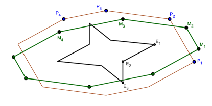
Figure 4: A polygon $M$ and its $P-$evolute $E$

This definition is the discrete version of the evolute in Evolutes . Now, $E$ is a $Q$-polygon, since

$$\Delta_{i}E=\left(M_{i+1}-r_{i+1}P_{i+1}\right)-\left(M_{i+1}-r_{i}P_{i+1}\right)=-\Delta_{i}r\cdot P_{i+1}=\alpha_{i}\Delta_{i}r\cdot\Delta_{i}Q$$

This means we can represent $E$ by its curvature radii with respect to $Q$, namely

$$s_{i}=\alpha_{i}\Delta_{i}r$$ (9)

So, using the radius representation, the evolute process $E_{P}:L_{P}\rightarrow L_{Q}$ is a linear transformation, whose $2n\times 2n$ matrix can be explicitly written as

$$E_{P}=\left[\begin{array}[c]{cccccc}-\alpha_{1}&\alpha_{1}&0&...&0&0\\ 0&-\alpha_{2}&\alpha_{2}&...&0&0\\ 0&0&-\alpha_{3}&...&0&0\\ \vdots&\vdots&\vdots&\ddots&\vdots&\vdots\\ 0&0&0&...&-\alpha_{2n-1}&\alpha_{2n-1}\\ \alpha_{2n}&0&0&...&0&-\alpha_{2n}\end{array}\right]$$

In order to characterize it geometrically, we need:

Definition 6

Given a periodic $P$-polygon $M$ represented by the radius vector $\vec{r}$, its (signed) $Q$-length is

$$L_{Q}\left(M\right)=\left\langle r,\mathbf{1}\right\rangle_{P}=\sum_{i=1}^{2n}\frac{r_{i}}{\beta_{i}}$$

which is the signed length of (one period of) $M$, taking $Q$ as the unit ball, since (from Eq. 2)

$$\Delta_{i}M=r_{i}\Delta_{i}P=\frac{r_{i}}{\beta_{i}}\cdot Q_{i}$$

Similarly, given a periodic $Q$-polygon $N$ represented by $\vec{s}$, its (signed) $P$-length is

$$L_{P}\left(N\right)=\left\langle s,\mathbf{1}\right\rangle_{Q}=\sum_{i=1}^{2n}\frac{s_{i}}{\alpha_{i}}$$

which is the signed length of $N$, taking $P$ as the unit ball, since

$$\Delta_{i}N=s_{i}\Delta_{i}Q=-\frac{s_{i}}{\alpha_{i}}\cdot P_{i+1}$$

Proposition 3

The image of $E_{P}$ is the space of all $Q$-polygons of zero $P$-length, and its kernel is $B_{P}$.

Proof

The kernel is easy:

$$s_{i}=0\Leftrightarrow\Delta_{i}r=0\Leftrightarrow r=\lambda\mathbf{1}$$

so we know that $rank\left(E_{P}\right)=2n-1$. Now, the $P$-length of the evolute $E$ is

$$L_{P}\left(E\right)=\sum_{i=1}^{2n}\frac{s_{i}}{\alpha_{i}}=\sum_{i=1}^{2n}\Delta_{i}r=0$$

and since the condition $L_{P}\left(N\right)=0$ determines a subspace of dimension $2n-1$ as well, we conclude it must be the whole image of $E_{P}$. ∎

4.2 Double evolutes

But why stop there? If $E$ is a $Q$-polygon, we can find the evolute of $E$ taking $Q$ as the new reference ball! Namely, we find a new curve $F$ given by:

$$F_{i+1}=E_{i+1}-s_{i}Q_{i+1}=E_{i}-s_{i}Q_{i}$$

where we shifted the indices in $F$ to compensate for the two forward differences we have taken. We have

$$\Delta_{i}F=\left(E_{i}-s_{i}Q_{i}\right)-\left(E_{i}-s_{i-1}Q_{i}\right)=-\nabla_{i}s\cdot Q_{i}=-\beta_{i}\nabla_{i}s\cdot\Delta_{i}P$$

so $F$ is a $P$-polygon again! The matrix of this second evolute transform $E_{Q}:L_{Q}\rightarrow L_{P}$ is

$$E_{Q}=\left[\begin{array}[c]{cccccc}-\beta_{1}&0&0&...&0&\beta_{1}\\ \beta_{2}&-\beta_{2}&0&...&0&0\\ 0&\beta_{3}&-\beta_{3}&...&0&0\\ \vdots&\vdots&\vdots&\ddots&\vdots&\vdots\\ 0&0&0&...&-\beta_{2n-1}&0\\ 0&0&0&...&\beta_{2n}&-\beta_{2n}\end{array}\right]$$

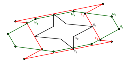
Figure 5: A polygon $M$ and its double evolute $F$

Definition 7

With the notation above, $F$ is the double evolute of $M$. Explicitly, $F$ is the curve whose curvature radii are:

$$t_{i}=-\beta_{i}\nabla_{i}s=-\beta_{i}\nabla_{i}\left(\alpha_{i}\Delta_{i}r\right)$$

so the matrix of the double evolute transform $T_{P}$ is

$$T_{P}=E_{Q}E_{P}=\left[\begin{array}[c]{ccccc}\beta_{1}\left(\alpha_{1}+\alpha_{2n}\right)&-\alpha_{1}\beta_{1}&0&...&-\alpha_{2n}\beta_{1}\\ -\alpha_{1}\beta_{2}&\beta_{2}\left(\alpha_{2}+\alpha_{1}\right)&-\alpha_{2}\beta_{2}&...&0\\ 0&-\alpha_{2}\beta_{3}&\beta_{3}\left(\alpha_{3}+\alpha_{2}\right)&...&0\\ \vdots&\vdots&\vdots&\ddots&\vdots\\ 0&0&0&...&-\alpha_{2n-1}\beta_{2n-1}\\ -\alpha_{2n}\beta_{2n}&0&0&...&\beta_{2n}\left(\alpha_{2n}+\alpha_{2n-1}\right)\end{array}\right]$$ (10)

We quickly note that $T_{P}$ is invariant by ball rescaling, since a rescaling on $P$ implies in the reverse scaling on $Q$. We are now ready to justify our choices of inner products:

Proposition 4

For any vectors $\vec{r}\in L_{P}$ and $\vec{w}\in L_{Q}$, we have

$$\left\langle E_{P}\vec{r},\vec{w}\right\rangle_{Q}=\left\langle\vec{r},E_{Q}\vec{w}\right\rangle_{P}$$

that is, $E_{Q}=E_{P}^{\ast}$ with this choice of inner products.

Proof

Just write

$$\left\langle E_{P}\vec{r},\vec{w}\right\rangle_{Q} =\sum_{i=1}^{2n}\frac{\alpha_{i}\Delta_{i}r}{\alpha_{i}}\cdot w_{i}=\sum_{i=1}^{2n}\Delta_{i}r\cdot w_{i}$$

$$\left\langle\vec{r},E_{Q}\vec{w}\right\rangle_{P} =\sum_{i=1}^{2n}\frac{r_{i}}{\beta_{i}}\cdot\left(-\beta_{i}\nabla_{i}w\right)=-\sum_{i=1}^{2n}r_{i}\nabla_{i}w$$

and the two sums are just rearrangements of each other. ∎

Proposition 5

$T_{P}$ is self-adjoint (therefore non-negative), and $C_{P}$ is invariant by $T_{P}$.

Proof

The first statement follows directly from $T_{P}=E_{P}^{\ast}E_{P}$. More explicitly, we have

$$\left\langle T_{P}r,r\right\rangle_{P}=\sum_{i=1}^{2n}r_{i}^{2}\left(\beta_{i}+\beta_{i-1}\right)-\sum_{i=1}^{2n}2\beta_{i}r_{i}r_{i+1}=\sum_{i=1}^{2n}\beta_{i}\left(r_{i}-r_{i+1}\right)^{2}\geq 0$$ (11)

with equality if, and only if, $r$ is a multiple of $\mathbf{1}$ (remember that $\beta_{i}>0$ from Eq. 4). The second fact is geometrically clear, but we also offer an algebraic proof: just remember that $C_{P}$ is defined by $\sum r_{i}\cdot\Delta_{i}P=0$. But the expression on the left side remains invariant under the evolute transform, since

$$\sum r_{i}\cdot\Delta_{i}P=-\sum\Delta_{i}r\cdot P_{i+1}=-\sum\frac{s_{i}}{\alpha_{i}}P_{i+1}=\sum s_{i}\cdot\Delta_{i}Q\text{.}{}$$

5 Discrete cycloids

Definition 8

A discrete cycloid is a polygonal line $M$ which is homothetic to its double evolute.

In other words, we want

$$\vec{t}=T_{P}\vec{r}=\lambda\vec{r}\text{,}$$

or, in operator notation,

$$\beta_{i}\nabla_{i}\left(\alpha_{i}\Delta_{i}r\right)+\lambda r_{i}=0$$ (11)

for some constant $\lambda$ – an eigenvalue problem!

Example 1 (Regular Polygons)

If $P$ is a regular polygon with $2n$ sides, then so is $Q$. Let $\gamma=\frac{\pi}{2n}$. We might as well rescale $P$ so $P$ and $Q$ are congruent to each other – explicitly, this happens when

$$\left|P_{i}\right|=\left|Q_{i}\right|=\frac{1}{\sqrt{\cos\gamma}}\Rightarrow\alpha_{i}=\beta_{i}=\frac{1}{2\sin\gamma}\text{.}$$

So in this case the double evolute transform

$$T_{P}=\frac{1}{4\sin^{2}\gamma}\left[\begin{array}[c]{cccccc}2&-1&0&...&0&-1\\ -1&2&-1&...&0&0\\ 0&-1&2&...&0&0\\ \vdots&\vdots&\vdots&\ddots&\vdots&\vdots\\ 0&0&0&...&2&-1\\ -1&0&0&...&-1&2\end{array}\right]$$

is a discrete convolution! One can verify directly that

$$\vec{c}_{k}=\left(1,\cos 2k\gamma,\cos 4k\gamma,...,\cos 2\left(2n-1\right)k\gamma\right);\ k=0,1,2,...,2n-1$$ (12)

are eigenvectors, since for $\phi\in\left\{0,2k\gamma,4k\gamma,...\right\}$:

$$2\cos\phi-\cos\left(\phi+2k\gamma\right)-\cos\left(\phi-2k\gamma\right)=2\left(1-\cos 2k\gamma\right)\cos\phi=4\sin^{2}k\gamma\cos\phi$$

In other words, the eigenvalues are

$$\lambda_{k}=\frac{\sin^{2}k\gamma}{\sin^{2}\gamma}$$

for $k=0,1,2,...,2n-1$. Since $\lambda_{k}=\lambda_{2n-k}$, all of them are double eigenvalues, except for $\lambda_{0}=0$ and $\lambda_{n}=\csc^{2}\gamma$. Also, note that $\vec{c}_{k}\in S_{P}$ if $k$ is even, and $\vec{c}_{k}\in A_{P}$ if $k$ is odd. In other words, if we rename the pair $\left(\lambda_{k},\lambda_{n-k}\right)$ as $\left(\lambda_{k}^{1},\lambda_{k}^{2}\right)$ for $k=1,2,...,n-1$, the eigenvalues can be ordered this way:

$$\lambda_{0}\left(=0\right)<\lambda_{1}^{1}=\lambda_{1}^{2}=1<\lambda_{2}^{1}=\lambda_{2}^{2}<\lambda_{3}^{1}=\lambda_{3}^{2}<...\lambda_{n-1}^{1}=\lambda_{n-1}^{2}<\lambda_{n}\left(=\csc^{2}\gamma\right)$$

Our goal is now to discover which parts of the spectral structure above remain true in the general case. Before we do that, let us rephrase our problem in a slightly different way – as a recurrence.

5.1 The half-turn transform

Once a candidate value for $\lambda$ is given, we can see our problem as a recurrence on the coordinates of $\vec{r}$, namely

$$r_{k+1}=\left(1+\frac{\alpha_{k-1}}{\alpha_{k}}-\frac{\lambda}{\alpha_{k}\beta_{k}}\right)r_{k}-\frac{\alpha_{k-1}}{\alpha_{k}}r_{k-1}\text{ \ \ \ }\left(k=2,3,...\right)$$ (13)

or, in matricial form

$$\left[\begin{array}[c]{c}r_{k}\\ r_{k+1}\end{array}\right]=S_{k}\left(\lambda\right)\left[\begin{array}[c]{c}r_{k-1}\\ r_{k}\end{array}\right]\text{ where }S_{k}\left(\lambda\right)=\left[\begin{array}[c]{cc}0&1\\ -\frac{\alpha_{k-1}}{\alpha_{k}}&1+\frac{\alpha_{k-1}}{\alpha_{k}}-\frac{\lambda}{\alpha_{k}\beta_{k}}\end{array}\right]$$ (14)

Since we want a solution $\vec{r}\in L_{P}$, the trick is to find special values of $\lambda$, $r_{1}$ and $r_{2}$ such that $r_{2n+1}=r_{1}$ and $r_{2n+2}=r_{2}$ in this recurrence. Actually, in order to separate symmetric from anti-symmetric solutions, we should stop half-way and check the relationship between $\left(r_{1},r_{2}\right)$ and $\left(r_{n+1},r_{n+2}\right)$.

Definition 9

Given $\lambda\in\mathbb{R}$, the half-turn transform $H_{\lambda}$ is the linear transformation which takes $\vec{\rho}=\left(r_{1},r_{2}\right)\in\mathbb{R}^{2}$ to $H_{\lambda}\vec{\rho}=\left(r_{n+1},r_{n+2}\right)\in\mathbb{R}^{2}$ according to the recurrence (13) above. In other words

$$H_{\lambda}=S_{n+1}\left(\lambda\right)\cdot S_{n}\left(\lambda\right)\cdot...\cdot S_{2}\left(\lambda\right)\text{.}$$

Though $H_{\lambda}$ depends on our index choice (for example, $H_{\lambda}$ does not necessarily take $\left(r_{2},r_{3}\right)$ to $\left(r_{n+2},r_{n+3}\right)$), we note that $H_{\lambda}$ does take $\left(r_{n+1},r_{n+2}\right)$ to $\left(r_{2n+1},r_{2n+2}\right)$, because of the $n$-periodicity of the sequences $\alpha$ and $\beta$. Now we can summarize:

• ”Finding an eigenvector $\vec{r}\in L_{P}$ of $T_{P}$ (for the eigenvalue $\lambda$)” is equivalent to
  ”finding an eigenvector $\vec{\rho}\in\mathbb{R}^{2}$ of $H_{\lambda}^{2}$ (for the eigenvalue $1$)”;

• ”Finding an eigenvector $\vec{r}\in S_{P}$ of $T_{P}$ (for the eigenvalue $\lambda$)” is equivalent to
  ”finding an eigenvector $\vec{\rho}\in\mathbb{R}^{2}$ of $H_{\lambda}$ (for the eigenvalue $1$)”;

• ”Finding an eigenvector $\vec{r}\in A_{P}$ of $T_{P}$ (for the eigenvalue $\lambda$)” is equivalent to
  ”finding an eigenvector $\vec{\rho}\in\mathbb{R}^{2}$ of $H_{\lambda}$ (for the eigenvalue $-1$)”.

Proposition 6

For any $\lambda\in\mathbb{R}$

$$\det H_{\lambda}=1$$

This restricts $H_{\lambda}$ to six possibilities, according to the geometric multiplicity of its eigenvalues:
Case $1$. If $H_{\lambda}=I$, then $\lambda$ is a double eigenvalue of $T_{P}$, and both its eigenvectors are in $S_{P}$.
Case $2$. If $H_{\lambda}=-I$, then $\lambda$ is a double eigenvalue of $T_{P}$, and both its eigenvectors are in $A_{P}$.
Case $3$. If $H_{\lambda}$ has a single eigenvalue $1$, then $\lambda$ is a single eigenvalue of $T_{P}$, with its eigenvector in $S_{P}$.
Case $4$. If $H_{\lambda}$ has a single eigenvalue $-1$, then $\lambda$ is a single eigenvalue of $T_{P}$, with its eigenvector in $A_{P}$.
Case $5$. If $H_{\lambda}$ has two distinct real eigenvalues $\mu$ and $\mu^{-1}$, then $\lambda$ is not an eigenvalue of $T_{P}$.
Case $6$. If $H_{\lambda}$ has two complex eigenvalues $e^{\pm i\theta}$, then $\lambda$ is not an eigenvalue of $T_{P}$.

Proof

The determinant follows directly from

$$\det S_{k}\left(\lambda\right)=\frac{\alpha_{k-1}}{\alpha_{k}}$$

and the symmetry of our ball ($\alpha_{n+1}=\alpha_{1}$). The existence of the eigenvectors in cases $1$-$4$ follows from the observation before the proposition – we just have to make sure there are no other eigenvectors of $H_{\lambda}^{2}$ in cases $3$-$6$.
In cases $3$ and $4$, we have

$$H_{\lambda}\approx\left[\begin{array}[c]{cc}\pm 1&1\\ 0&\pm 1\end{array}\right]\Rightarrow H_{\lambda}^{2}\approx\left[\begin{array}[c]{cc}1&\pm 2\\ 0&1\end{array}\right]$$

which clearly has only one eigenvalue $1$. In case $5$ the eigenvalues of $H_{\lambda}^{2}$ are $\mu^{2}$ and $\mu^{-2}$, and neither is $1$. Finally, in case $6$:

$$H_{\lambda}\approx R_{\theta}\Rightarrow H_{\lambda}^{2}\approx R_{2\theta}$$

where $R_{\theta}$ is a rotation of angle $\theta$ in the plane. Since $\theta$ is not a multiple of $\pi$, $H_{\lambda}^{2}$ has no eigenvalues. ∎

Now we go back to the structure of the eigenvalues of the double evolute $T_{P}$.

5.2 Eigenvalue $0$

We already know from Eq. 11 that

$$\left\langle T_{P}r,r\right\rangle=\sum_{i=1}^{2n}\beta_{i}\left(r_{i}-r_{i+1}\right)^{2}$$

so $T_{P}\vec{r}=0$ if and only if $\vec{r}=\gamma\mathbf{1.}$ In other words, $Ker\left(T_{P}\right)=B_{P}$, and $0$ is always a single eigenvalue of $T_{P}$.

5.3 Double eigenvalue $1$

Surprisingly, we can state very explicitly a pair of eigenvectors associated to the $1$ eigenvalue of $T_{P}$ in the general case:

Proposition 7

Let $X$ be any non-zero fixed vector in $\mathbb{R}^{2}$. Then the vector $u$ defined by

$$u_{i}=\left[X,Q_{i}\right]\ \ \ \ \ \ \left(i=1,2,...,2n\right)$$

satisfies $T_{P}u=u$. Moreover, the $P$-polygon determined by $u$ does not close, that is, $\vec{u}\notin C_{P}$.

Proof

Using our previous notation and remembering 2, we calculate directly

$$s_{i} =\alpha_{i}\Delta_{i}r=\alpha_{i}\left[X,\Delta_{i}Q\right]=-\left[X,P_{i+1}\right]$$

$$t_{i} =-\beta_{i}\nabla_{i}s=\beta_{i}\left[X,\Delta_{i}P\right]=\left[X,Q_{i}\right]$$

Now the ”drift” of the $P$-polygon after one turn (see Eqs. 6 and 2) is

$$D=\sum_{i=1}^{2n}u_{i}\Delta_{i}P=\sum_{i=1}^{2n}\frac{\left[X,Q_{i}\right]}{\beta_{i}}Q_{i}\text{.}$$

So the component of the drift in the direction orthogonal to $X$ is

$$\left[X,D\right]=\sum_{i=1}^{2n}\frac{\left[X,Q_{i}\right]^{2}}{\beta_{i}}$$

which is clearly positive, since $\beta_{i}>0$ for all $i$ and $X\neq\vec{0}$. In other words, the ”drift” cannot be $\vec{0}$, and the $P$-polygon does not close. ∎

Since there are $2$ degrees of freedom in the choice of $X$, that gives us a $2$ dimensional space of eigenvectors. More explicitly, one can define vectors $u^{\prime}$ and $u^{\prime\prime}$ by taking

$$u_{i}^{\prime} =\left[Q_{1},Q_{i}\right]$$

$$u_{i}^{\prime\prime} =\left[Q_{2},Q_{i}\right]$$

which are clearly linearly independent: $u^{\prime}=\left(0,\left[Q_{1},Q_{2}\right],...\right)$ and $u^{\prime\prime}=\left(\left[Q_{2},Q_{1}\right],0,...\right)$. Also, from the symmetry of $Q$, we see that such solutions satisfy $u_{i+n}=-u_{i}$, so we have

$$Ker\left(T_{P}-I\right)\subseteq A_{P}$$

Actually, consider the following general discrete Sturm-Liouville equation presented in WangShi :

$$\nabla_{i}\left(a_{i}\Delta_{i}u\right)+\left(\lambda b_{i}-c_{i}\right)u_{i}=0$$ (15)

where $a_{i},b_{i}>0$ and $c_{i}$ are given $n$-periodic sequences and we want to find the eigenvalue $\lambda$ and the $2n$-periodic sequence $u$. A class of such equations can be interpreted as cycloid problems:

Proposition 8

Suppose the problem described above has $c_{i}=0$ and a double eigenvalue $1$. Then there is a symmetric, locally convex ball $P$ such that

$$a_{i}=\alpha_{i}=\frac{1}{\left[Q_{i},Q_{i+1}\right]}\text{ and }b_{i}=\frac{1}{\beta_{i}}=\left[P_{i},P_{i+1}\right]$$

so Eq. 15 becomes the cycloid problem in Eq. 11.

Proof

Let $u=x$ and $u=y$ be two linearly independent solutions of 15 associated to the eigenvalue $1$. Take the sequence of points $Q_{i}=\left(x_{i},y_{i}\right)$ in the plane. Looking at one coordinate at a time, it is easy to see that

$$\nabla_{i}\left(a_{i}\Delta_{i}Q\right)=-b_{i}Q_{i}\Rightarrow\nabla_{i}a\cdot\Delta_{i}Q-a_{i-1}\cdot\delta_{i}^{2}Q=-b_{i}Q_{i}$$

so, remembering that

$$\left[\delta_{i}^{2}Q,\Delta_{i}Q\right]=\left[\Delta_{i}Q-\nabla_{i}Q,\Delta_{i}Q\right]=\left[\Delta_{i}Q,\nabla_{i}Q\right]$$

we can write

$$a_{i-1}\left[\delta_{i}^{2}Q,\Delta_{i}Q\right]=b_{i}\left[Q_{i},\Delta_{i}Q\right]\Rightarrow a_{i-1}\left[\Delta_{i}Q,\nabla_{i}Q\right]=b_{i}\left[Q_{i},Q_{i+1}\right]$$ (16)

Note that, if we had $\left[\Delta_{i}Q,\nabla_{i}Q\right]=0$ above, that would force $\left[Q_{i},Q_{i+1}\right]=0$, which is not possible since $x$ and $y$ are linearly independent. Now, aiming towards Eq. 2, we define

$$P_{i}=-\frac{\nabla_{i}Q}{\left[Q_{i-1},Q_{i}\right]}$$

so we can compute

$$\left[\nabla_{i}Q,\Delta_{i}Q\right]=\left[P_{i},P_{i+1}\right]\cdot\left[Q_{i-1},Q_{i}\right]\cdot\left[Q_{i},Q_{i+1}\right]$$

That allows us to rewrite Eq. 16 as

$$a_{i-1}\left[Q_{i-1},Q_{i}\right]=\frac{b_{i}}{\left[P_{i},P_{i+1}\right]}\text{,}$$

so, rescaling $Q$ if necessary, we may assume $a_{i-1}=\alpha_{i-1}=\frac{1}{\left[Q_{i-1},Q_{i}\right]}$ and $b_{i}=\frac{1}{\beta_{i}}=\left[P_{i},P_{i+1}\right]$, as claimed. Since the sequences $a_{i}$ and $b_{i}$ are positive and $n$-periodic, we can now see that $P$ and $Q$ are locally convex and symmetric. ∎

5.4 No triple eigenvalues

Proposition 9

If $\lambda$ is any eigenvalue, then

$$\dim\left(Ker\left(T_{P}-\lambda I\right)\right)\leq 2$$

Proof

This is a direct consequence of the recurrence – given $\lambda$, once the values $r_{1}$ and $r_{2}$ are chosen, recurrence 13 determines all other coordinates of $\vec{r}$. Or, in other words, $H_{\lambda}^{2}$ has at most $2$ eigenvectors associated to the eigenvalue $1$. ∎

5.5 No eigenvalues with eigenvectors in both $S_{P}$ and $A_{P}$

Proposition 10

The restrictions $T_{P}|_{A_{P}}$ and $T_{P}|_{S_{P}}$ have no common eigenvalues.

Proof

If a eigenvalue $\lambda$ had eigenvectors in both $A_{P}$ and $S_{P}$, the corresponding half-way transform $H_{\lambda}$ would have both $1$ and $-1$ as eigenvalues. Since $\det H_{\lambda}=1$, this is impossible. ∎

Putting all pieces together, we have the main result of this section:

5.6 The spectral structure of the double evolute

Proposition 11

The eigenvalues of $T_{P}$ (in Eq. 10) can be ordered as

$$\lambda_{0}\left(=0\right)<\lambda_{1}^{1}=\lambda_{1}^{2}\left(=1\right)<\lambda_{2}^{1}\leq\lambda_{2}^{2}<\lambda_{3}^{1}\leq\lambda_{3}^{2}<...\lambda_{n-1}^{1}\leq\lambda_{n-1}^{2}<\lambda_{n}$$ (17)

where $\lambda_{k}^{1,2}$ are eigenvalues of $T_{P}|_{A_{P}}$ if $k$ is odd and $0$ and $\lambda_{k}^{1,2}$ are eigenvalues of $T_{P}|_{S_{P}}$ if $k$ is even.

Proof

Any $P$-ball can be continuously deformed towards a $2n$-regular polygon (being kept convex and symmetric in the process). Throughout the process, the eigenvalues of $T_{P}$ change continuously, and its eigenvectors (always in $A_{P}$ or $S_{P}$) can also be chosen to change continuously. Now, the proposition above guarantees that eigenvalues corresponding to eigenvectors in distinct spaces (one in $A_{P}$, another in $S_{P}$) cannot ”switch places” through the process! Therefore, the ordering of the eigenvalues of $T_{P}$ (belonging to different spaces) must be the same as it is in the case of regular polygons! ∎

Remark 1

The above proposition begs the following question: can one hear the shape of a convex symmetric body? We mean, given a specific list of cycloid eigenvalues, are we able to determine the shape of the $P$-ball? Or, a slight variation on this question: if all eigenvalues are double, do we necessarily have a regular polygon?

Remark 2

Note that Eq. 7 can be rewritten in terms of the double evolute transform!

$$\vec{r}=\left(I-T_{P}\right)\vec{h}$$

So, let $\vec{r}$ be the radii associated to a closed cycloid, say, $T_{P}\vec{r}=\lambda\vec{r}$ with $\lambda\neq 1$. Taking $\vec{h}=\frac{1}{1-\lambda}\vec{r}$, we define a $P$-polygon whose radii vector is exactly $\vec{r}$, since

$$\left(I-T_{P}\right)\vec{h}=\frac{1}{1-\lambda}\vec{r}-\frac{\lambda}{1-\lambda}\vec{r}=\vec{r}\text{.}$$

This shows that the support function of a (correctly placed in the plane) closed cycloid is also an eigenvector of $T_{P}$. In other words, any closed $P$-polygon can be written as the Minkowski sum of $2n-2$ closed cycloids! Now, periodic support functions cannot represent open polygons like our open cycloids, hence our choice or primarily working with curvature radii.

5.7 Cusps

Definition 10

Given a periodic $P$-polygon $M$ represented by the radius vector $\vec{r}$, the orientation of its side $\Delta_{i}M$ is the sign of the corresponding radius $r_{i}$. A vertex $V$ of $M$ is a cusp if its neighbor (non-degenerate) sides have opposite orientations. Such cusp will be named ordinary if there is at most one degenerate side at $V$.

Such cusps have appeared at Schneider (where they were called strong corners). Geometrically, sides which meet at cusp are on opposite sides of the normal line $\left\{M_{i}+tP_{i};t\in\mathbb{R}\right\}$; algebraically, each cusp corresponds to a zero-crossing of the sequence $\left(r_{i}\right)_{i\in\mathbb{Z}}$. For example, a snippet $\left(...,-2,0,0,0,0,3,...\right)$ corresponds to one non-ordinary cusp, while $\left(...,2,0,2,...\right)$ is not a cusp at all.

Now, consider how the number of zero-crossings (per period) of a sequence $\vec{r}$ can change if $\vec{r}$ is changed continuously. One can create two cusps going from a ”$+0+$” subsequence to ”$+-+$” (or from ”$-0-$” to ”$-+-$”, of course); one can destroy two cusps reversing this process. Finally, many zero-crossings can be created at once if a sequence of consecutive $0$s is present (for example, from ”$+000+$” to ”$+-+-+$”). Outside of these situations, there is no way to create or destroy a cusp (it is possible to move it, of course, going from ”$++-$” to ”$+0-$” to ”$+--$”, but in each of these cases we have only one ordinary cusp). Under this light, the following proposition is important:

Proposition 12

In a cycloid, any zero entries in the radius vector must correspond to cusps; also, all cusps are ordinary.

Proof

This is a direct consequence of the recurrence 13: if $v_{k}=0$, then $v_{k+1}$ and $v_{k-1}$ must have opposite signs; if two consecutive sides were $0$, all of them would be $0$. ∎

Proposition 13

Given a $P$-ball with $2n$ sides, the number of cusps of its associated cycloids is respectively

$$0,2,2,4,4,6,6,...,2n-2,2n-2,2n$$

Proof

Once again, deform $P$ continuously towards a $2n-$regular polygon. Since ordinary cusps are stable with relation to changes in the radii vectors (as long as no consecutive zeroes occur), the previous proposition guarantees that each cycloid will have a constant number of cusps as the deformation takes place. Now it is just a matter of checking how many cusps each of the eigenvectors in Equation 12 has. ∎

6 Other periods

In the Euclidean plane, hypocycloids and epicycloids might take several turns to close. This suggests we could relax the periodicity condition (Eq. 5) on the curvature representation $\left(r_{i}\right)_{i\in\mathbb{Z}}$ of the polygonal line $M$ – requiring, instead, the sequence to be periodic with period $2mn$, say. Can we find discrete closed cycloids with other periods this way?

We claim that a big part of the analysis in such cases is already done! After all, we did not really use that the unit ball $P$ is a simple closed convex polygon – we only needed local convexity, as seen in Eqs. 4, so we could establish the positivity of $\alpha_{i}$ and $\beta_{i}$ (defined in Eq. 3). In other words, if one wants to find $2mn$-periodic cycloids with reference to a $2n$-ball $P$, one can instead look for $2mn$-periodic cycloids with reference to the $2mn$-ball which is determined by $P$ traversed $\mathbf{m}$ times (call this polygon $mP$).

So the reader will have the pleasure of re-reading this article from the beginning switching $P$ with $mP$, a polygon which goes $m$ times around the origin (two articles for the price of one!). All calculations in Section 2 are unchanged, except that indices go $i=1,2,...,2mn$. The new curvature radius space of Section 3 (that would be $L_{mP}$) has dimension $2mn$, and the corresponding spaces $S_{mP}$ and $A_{mP}$ are still orthogonal complements of each other. All calculations done in Section 4 still hold, but the matrices are $2mn\times 2mn$. Finally, all arguments in Section 5 still hold, with a few exceptions – first, our base case must change:

Example 2 (Regular Polygon traversed $m$ times)

If $P$ is a regular polygon with $2n$ sides, traversed $m$ times, then so is $Q$. Write $\alpha=\frac{\pi}{2n}$ and $\gamma=\frac{\pi}{2mn}$ and assume by rescaling that

$$\left|P_{i}\right|=\left|Q_{i}\right|=\frac{1}{\sqrt{\cos\alpha}}\Rightarrow\alpha_{i}=\beta_{i}=\frac{1}{2\sin\alpha}\text{.}$$

The double evolute transform is the same as before, except for the matrix size which now must be $2mn\times 2mn$:

$$T_{mP}=\frac{1}{4\sin^{2}\alpha}\left[\begin{array}[c]{cccccc}2&-1&0&...&0&-1\\ -1&2&-1&...&0&0\\ 0&-1&2&...&0&0\\ \vdots&\vdots&\vdots&\ddots&\vdots&\vdots\\ 0&0&0&...&2&-1\\ -1&0&0&...&-1&2\end{array}\right]$$

The eigenvectors are

$$\vec{d}_{k}=\left(1,\cos 2k\gamma,\cos 4k\gamma,...,\cos 2\left(2mn-1\right)k\gamma\right);\ k=0,1,2,...,2mn-1$$

and the eigenvalues are

$$\sigma_{k}=\frac{\sin^{2}k\gamma}{\sin^{2}\alpha}$$

for $k=0,1,2,...,2mn-1$. Again, $\sigma_{k}=\sigma_{2mn-k}$, so all of them are double eigenvalues, except for $\sigma_{0}=0$ and $\sigma_{mn}=\csc^{2}\alpha$. Renaming $\left(\sigma_{k},\sigma_{2mn-k}\right)$ as $\left(\sigma_{k}^{1},\sigma_{k}^{2}\right)$ for $k=1,2,...,mn-1$, the eigenvalues can be ordered this way:

$$\sigma_{0}\left(=0\right)<\sigma_{1}^{1}=\sigma_{1}^{2}<\sigma_{2}^{1}=\sigma_{2}^{2}<...<\sigma_{m}^{1}=\sigma_{m}^{2}(=1)<...<\sigma_{mn-1}^{1}=\sigma_{mn-1}^{2}<\sigma_{mn}\left(=\csc^{2}\alpha\right)$$

Each eigenvector has only regular cusps. In fact, taking $k=0,1,2,...,mn$, we can see that the number of cusps in $\vec{d}_{k}$ is exactly $2k$. So the number of cusps in each cycloid can be ordered (correspondingly to the eigenvalues) in the list

$$0,2,2,4,4,...,2mn-2,2mn-2,2mn\text{.}$$

Finally, if $k=jm$ ($j=1,2,...,n$) then $k\gamma=j\alpha$, and

$$\vec{d}_{jm}=\vec{c}_{j}\text{ and }\sigma_{jm}^{1,2}=\lambda_{j}^{1,2}$$

where $\lambda$ and $\vec{c}$ are the eigenvalues/vectors in the case the polygon was traversed just once (see Example in page 1).

So the following (partial!) result is easily obtained as before:

Proposition 14

When the unit ball is traversed $m$ times, the eigenvalues of the double evolute transform can be ordered as

$$\sigma_{0}\left(=0\right)<\sigma_{1}^{1}\leq\sigma_{1}^{2}<\sigma_{2}^{1}\leq\sigma_{2}^{2}<...<\sigma_{m}^{1}=\sigma_{m}^{2}=1<...<\sigma_{mn-1}^{1}\leq\sigma_{mn-1}^{2}<\sigma_{mn}$$

where $\sigma_{k}^{1,2}$ are eigenvalues of $T_{mP}|_{A_{mP}}$ if $k$ is odd and $0$ and $\sigma_{k}^{1,2}$ are eigenvalues of $T_{mP}|_{S_{mP}}$ if $k$ is even. The number of cusps of the associated cycloids are respectively

$$0,2,2,4,4,...,2mn-2,2mn-2,2mn\text{.}$$

Proof

As before, start with a $2n-$regular polygon, traversed $m$ times around the origin, and deform it continuously towards $mP$. Since the eigenvalues $\sigma_{k}^{1,2}$ cannot switch places with $\sigma_{k+1}^{1,2}$ (that would imply an eigenvalue common to $A_{mP}$ and $S_{mP}$), the ordering above must be kept throughout. Similarly, since all cusps are kept ordinary throughout the deformation, their number must be constant in each eigenvector. ∎

6.1 From one turn to many turns

Our final goal this section is to relate the eigenvalues of $T_{mP}$ with the eigenvalues of $T_{P}$. To do that, we fully turn our attention to the half-turn transform, for now we have:

$$\left[\begin{array}[c]{c}r_{2mn+2}\\ r_{2mn+1}\end{array}\right]=H_{\lambda}^{2m}\left[\begin{array}[c]{c}r_{1}\\ r_{2}\end{array}\right]$$

So now we say:

• ”Finding an eigenvector $\vec{r}=\left(r_{1},r_{2},...,r_{2mn-1}\right)\in L_{mP}$ of $T_{mP}$ (for the eigenvalue $\lambda$)” is equivalent to
  ”finding an eigenvector $\vec{\rho}=\left(r_{1},r_{2}\right)\in\mathbb{R}^{2}$ of $H_{\lambda}^{2m}$ (for the eigenvalue $1$)”;

Adapting proposition 6, we have:

Proposition 15

Let $\lambda\in\mathbb{R}$. We can once again classify $\lambda$ as an eigenvalue of $T_{mP}$ according to the geometric multiplicity of the eigenvalues of $H_{\lambda}$:
Case $1$. If $H_{\lambda}=I$, then $\lambda$ is a double eigenvalue of $T_{mP}$, and both its eigenvectors are in $S_{mP}$.
Case $2$. If $H_{\lambda}=-I$, then $\lambda$ is a double eigenvalue of $T_{mP}$, and both its eigenvectors are in $A_{mP}$.
Case $3$. If $H_{\lambda}$ has a single eigenvalue $1$, then $\lambda$ is a single eigenvalue of $T_{mP}$, with its eigenvectors in $S_{mP}$.
Case $4$. If $H_{\lambda}$ has a single eigenvalue $-1$, then $\lambda$ is a single eigenvalue of $T_{mP}$, with its eigenvectors in $A_{mP}$.
Case $5$. If $H_{\lambda}$ has two distinct real eigenvalues $\mu$ and $\mu^{-1}$, then $\lambda$ is not an eigenvalue of $T_{mP}$.
Case $6a$. If $H_{\lambda}$ has two complex eigenvalues $e^{\pm i\theta}$ and $\theta$ is an even(odd) multiple of $\frac{\pi}{m}$, then $\lambda$ is a double eigenvalue of $T_{mP}$, with its eigenvectors in $S_{mP}$($A_{mP}$).
Case $6b$. If $H_{\lambda}$ has two complex eigenvalues $e^{\pm i\theta}$ and $\theta$ is not a multiple of $\frac{\pi}{m}$, then $\lambda$ is not an eigenvalue of $T_{mP}$.

Proof

Cases $1$ and $2$ are as before. Cases $3$ and $4$ are also very much the same, since

$$H_{\lambda}\approx\left[\begin{array}[c]{cc}\pm 1&1\\ 0&\pm 1\end{array}\right]\Rightarrow H_{\lambda}^{2m}\approx\left[\begin{array}[c]{cc}1&\pm 2m\\ 0&1\end{array}\right]$$

which clearly has only one eigenvalue $1$. In case $5$ the eigenvalues of $H_{\lambda}^{2m}$ are $\mu^{2m}$ and $\mu^{-2m}$, and neither is $1$. Now, in case $6$:

$$H_{\lambda}\approx R_{\theta}\Rightarrow H_{\lambda}^{2m}\approx R_{2m\theta}$$

and that is why we have to separate it further: if $2m\theta$ is a multiple of $\pi$, then $H_{\lambda}^{2m}=\pm I$ and we are back to cases $1$ or $2$; otherwise, $H_{\lambda}^{2m}$ has no eigenvalues. ∎

Do note that the half-turn transform $H_{\lambda}$ is exactly the same here as it was in the ”one turn” case! So cases $1$-$5$ happen just as often here as they did before, and with the same values for $\lambda$ – they account for $2m$ of the $2mn$ eigenvalues we found! So all the new eigenvalues must come from case $6a$… Can we figure out their ordering with relation to the ”old” eigenvalues? Indeed we can – we just need another continuity argument.

Proposition 16

Let the specter of $T_{P}$ be as denoted in 17. The eigenvalue(s) $\mu$ (and $\mu^{-1}$) of $H_{\lambda}$ depend on $\lambda$ in the following way:
a) If $\lambda_{k}^{2}<\lambda<\lambda_{k+1}^{1}$, then $H_{\lambda}$ has two complex eigenvalues (as in case $6$). In fact, as $\lambda$ grows from $\lambda_{k}^{2}$ to $\lambda_{k+1}^{1}$, the eigenvalues $\mu$ and $\mu^{-1}$ go through all values in the complex unit circle exactly once.
b) If $\lambda_{k}^{1}<\lambda<\lambda_{k}^{2}$ or $\lambda<0$, then $H_{\lambda}$ has two distinct real eigenvalues (as in case $5$).

Proof

Just consider the positioning of $\mu$ in the complex plane in each of the $6$ cases we considered, as displayed in Figure 6:

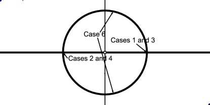
Figure 6: Where is $\mu$ in the complex plane?

Since $\mu$ varies continuously with $\lambda$ (and $\mu\neq 0$), in order to go from cases $1,3$ to $2,4$ (and vice-versa) we must go through all complex numbers in the circle $\left|\mu\right|=1$ (they do come in conjugate pairs, of course). So each interval of the kind $I_{k}=\left(\lambda_{k}^{2},\lambda_{k+1}^{1}\right)$ will contain at least $m-1$ values of $\lambda$ which correspond to the eigenvalues $e^{\pm i\theta}$ for $\theta=\frac{k\pi}{m}$ ($k=1,2,...,m-1$) of $H_{\lambda}$, as in case $6a$. Now, how do we know that each of these complex eigenvalues is visited only once as $\lambda$ varies in $I_{k}$? Every time $\lambda$ falls into case $6a$, such $\lambda$ is an eigenvalue of $T_{mP}$. Since there are $n$ such intervals $I_{k}$, and each interval already contains $m-1$ double eigenvalues, this already accounts for $2\left(m-1\right)n$ eigenvalues. If we now add the $\lambda_{k}^{1,2}$ themselves (there are $2n$ of them), which are also eigenvalues of $T_{mP}$, we are already crowded with all $2mn$ eigenvalues $T_{mP}$ could possibly have! So no other values of $\lambda$ can generate eigenvalues of $H_{\lambda}$ of the form $e^{\pm i\theta}$ where $\theta$ is any rational multiple of $\pi$. That proves not only that each complex eigenvalue is visited only once in each interval (a), but also shows that in (b) no new complex eigenvalues $\mu$ can appear – so while $\lambda\in\left(\lambda_{k}^{1},\lambda_{k}^{2}\right)$ or $\lambda<0$, we must keep $\mu$ real and different from $1$. ∎

We can now gather all information we have in one final proposition:

Proposition 17

The $2mn$ eigenvalues of $T_{mP}$ can be ordered the following way

$$\lambda_{0}\left(=0\right)$$

Proof

All the work is already done – just define $\lambda_{p}^{1,2}$ as the value of $\lambda$ which makes $H_{\lambda}$ have the eigenvalues $e^{\pm i\pi p}$ when the integer part of $p$ is even (that is, when you are moving from cases $1,3$ to $2,4$); or $e^{\pm i\pi\left(1-p\right)}$ otherwise. ∎

6.2 No periods!

What if we relax the periodicity condition even further: let us not require the list $\left\{r_{n}\right\}_{n\in Z}$ to be periodic. What then?

First of all, clearly the eigenvalues can now be any real number. After all, just pick any $\lambda\in\mathbb{R}$, any two values $r_{1}$, $r_{2}\in\mathbb{R}$ and apply recurrence 13 both backwards and forwards to create the complete list $\left\{r_{n}\right\}$. Moreover, if the number $\lambda$ you picked is any of the eigenvalues of $T_{mP}$ for some $m$, the list will be periodic of period $2mn$, as seen above (and, unless $\lambda=1$, the cycloid will close). Otherwise, we must have non-periodic cycloids! As such, one interesting phenomenon (which does not exist in the Euclidean case) can occur – a spiraling cycloid.

Figure 7: Two very different spiraling cycloids associated to the same $\lambda\approx 3.3$

Proposition 18

Suppose $\lambda_{n}^{1}<\lambda<\lambda_{n}^{2}$ or $\lambda<0$. Then the cycloids associated to $\lambda$ are unlimited.

Proof

Just remember that in this case, the eigenvalues associated to $H_{\lambda}$ can be written as $\mu$ and $\mu^{-1}$ where $\left|\mu\right|>1$. Writing $\vec{\rho}=\left(r_{1},r_{2}\right)=c_{1}\rho_{1}+c_{2}\rho_{2}$ where $\rho_{1}$ and $\rho_{2}$ are the respective eigenvectors of $H_{\lambda}$ we have $H_{\lambda}^{m}\vec{\rho}=c_{1}\mu^{m}\rho_{1}+c_{2}\mu^{-m}\rho_{2}$. If $c_{1}\neq 0$, we have $\left|r_{mn+1}\right|\rightarrow\infty$ as $m\rightarrow\infty$; if $c_{1}=0$, then $\left|r_{mn+1}\right|\rightarrow\infty$ as $m\rightarrow-\infty$. Either way, the cycloid is unlimited. ∎

7 A Four Vertex Theorem

In differential geometry, a ”vertex” of a curve is a point where the curvature reaches a local extremum. We want to show that any closed $P$-polygon has at least $4$ vertices… of this other kind, which needs to be defined.

Definition 11

An edgex of a $P$-polygon is a collection of adjacent sides whose (equal) curvatures correspond to a strict extremum of the sequence of radii in $\vec{r}$. In other words, an edgex is a zero-crossing of $\Delta\vec{r}$.

To clarify, if the radii vector is $\left(...,1,2,3,3,3,2,2,...\right)$, we count that sequence of threes as one edgex, but if the sequence were $\left(....,1,2,3,3,3,4,5,...\right)$ we see no edgex at all in this part of the polygon. So we are ready to state our ”four edgex theorem”, which adapts the reasoning in Taba :

Proposition 19

Any closed convex polygon $M$ (which is not homothetic to the $P$-ball) has at least four edgices. If $M$ has constant $P$-width, it must have at least six edgices.

Proof

Take the radii vector $\vec{r}\in C_{P}$ associated to $M$, and decompose it as

$$\vec{r}=\vec{r}_{0}+\vec{r}_{2}^{1}+\vec{r}_{2}^{2}+\vec{r}_{3}^{1}+\vec{r}_{3}^{2}+...+\vec{r}_{n-1}^{1}+\vec{r}_{n-1}^{2}+\vec{r}_{n}$$

where each $\vec{r}_{i}^{j}$ is a cycloid associated to the eigenvalue $\lambda_{i}^{j}$ (note that $i\neq 1;$ suppose for now that $\vec{r}_{2}^{1}\neq\vec{0}$). Since $\vec{r}_{0}$ is a multiple of $\mathbf{1}$, it does not alter its number of local extrema, so we may discard it completely. We can define a double involute of $M$ as the $P$-polygon with radii vector given by

$$I_{P}\vec{r}=\frac{\vec{r}_{2}^{1}}{\lambda_{2}^{1}}+\frac{\vec{r}_{2}^{2}}{\lambda_{2}^{2}}+...+\frac{\vec{r}_{n}}{\lambda_{n}}$$

Note that $T_{P}I_{P}\vec{r}=\vec{r}$ ($I_{P}$ is the pseudo-inverse of $T_{P}$). Now the key to the proof is to realize that every application of either evolute transform $E_{P}$ or $E_{Q}$ cannot decrease the number of edgices! This should be clear from Eq. 9 – since $s_{i}=\alpha_{i}\Delta_{i}r$, each edgex of $\vec{r}$ must correspond to a zero crossing of $\vec{s}$, and between two consecutive zero crossings of $\vec{s}$ we must have an edgex of $\vec{s}$! In other words, since $\vec{r}$ is the double evolute of $I_{P}\vec{r}$, we conclude that $\vec{r}$ must have at least as many edgices as $I_{P}\vec{r}$. Now iterate $I_{P}$! So $\vec{r}$ has at least as many edgices as

$$I_{P}^{k}\vec{r}=\frac{\vec{r}_{2}^{1}}{\left(\lambda_{2}^{1}\right)^{k}}+\frac{\vec{r}_{2}^{2}}{\left(\lambda_{2}^{2}\right)^{k}}+...+\frac{\vec{r}_{n}}{\left(\lambda_{n}\right)^{k}}=\frac{1}{\left(\lambda_{2}^{1}\right)^{k}}\left(\vec{r}_{2}^{1}+\left(\frac{\lambda_{2}^{1}}{\lambda_{2}^{2}}\right)^{k}\vec{r}_{2}^{2}+...+\left(\frac{\lambda_{2}^{1}}{\lambda_{n}}\right)^{k}\vec{r}_{n}\right)$$

We might as well ignore the homothety of a factor of $\left(\lambda_{2}^{1}\right)^{k}$, and note that eventually this involute will be arbitrarily close to $\vec{r}_{2}^{1}$ – which is a cycloid with $4$ cusps, and therefore $4$ edgices (if $\lambda_{2}^{1}=\lambda_{2}^{2}$, just group together $\vec{r}_{2}^{1}$ and $\vec{r}_{2}^{2}$ to form a single cycloid with $4$ cusps and repeat the argument). If it so happens that $\vec{r}_{2}^{1}=\vec{r}_{2}^{2}=\vec{0}$, just repeat the argument using the first non-zero cycloid instead of $\vec{r}_{2}^{1}$, and the number of cusps will be even bigger. For example, if the initial curve has constant $P$-width, then it must live in $W_{P}=B_{P}\oplus D_{P}$; since we are ignoring the component $\vec{r}_{0}$, we have a vector in $D_{P}\subseteq A_{P}$, so the $\vec{r}_{2}$ components must be zero and the decomposition starts with $\vec{r}_{j}^{i}$ where $j\geq 3$ – a cycloid with $6$ cusps or more, and therefore $6$ edgices or more. ∎

References

- (1) M. Arnold, I. Izmestiev, D. Fuchs, S. Tabachnikov & E. Tsukerman, Iterating evolutes and involutes, http://arxiv.org/abs/1510.07742.
- (2) M. Craizer, R. Teixeira & V. Balestro, Closed cycloids in a normed plane (2016), http://arxiv.org/abs/1608.01651.
- (3) M. Craizer & H. Martini, Involutes of polygons of constant width in Minkowski planes, Ars Mathematica Contemporanea 11 (2016), 107–125.
- (4) M. Kac, Can one hear the shape of a drum?, Amer. Math. Monthly 73 (1966), 1–23.
- (5) R. Schneider, The middle hedgehog of a planar convex body, Beiträge Algebra Geom. (2016), 1–11.
- (6) S. Tabachnikov, A four vertex theorem for polygons, Amer. Math. Monthly 107 (2000), 830–833.
- (7) A. C. Thompson, Minkowski Geometry, Encyclopedia of Mathematics and its Applications, Vol. 63, Cambridge Univ. Press, Cambridge, 1996.
- (8) Y. Wang & Y. Shi, Eigenvalues of second-order difference equations with periodic and antiperiodic boundary conditions, J. Math. Anal. Appl. 309 (2005), 56–69.