Malliavin-based Multilevel Monte Carlo Estimators for Densities of Max-stable Processes

Abstract

We introduce a class of unbiased Monte Carlo estimators for the multivariate density of max-stable fields generated by Gaussian processes. Our estimators take advantage of recent results on exact simulation of max-stable fields combined with identities studied in the Malliavin calculus literature and ideas developed in the multilevel Monte Carlo literature. Our approach allows estimating multivariate densities of max-stable fields with precision $\varepsilon$ at a computational cost of order $O\left(\varepsilon^{-2}\log\log\log\left(1/\varepsilon\right)\right)$.

1 Introduction

Max-stable random fields arise as the asymptotic limit of suitably normalized maxima of many i.i.d. random fields. Intuitively, max-stable fields are utilized to study the extreme behavior of spatial statistics. For instance, if the logarithm of a precipitation field during a relatively short time span follows a Gaussian random field, then extreme precipitations over a long time horizon, which are obtained by taking the maximum at each location of many precipitation fields can be argued (if enough temporal independence can be assumed) to follow a suitable max-stable process. Precisely these types of applications in environmental science motivate the study of max-stable processes (see, for example, [2] for a recent study of this type).

To calibrate and estimate max-stable random fields, it is desirable to evaluate the density over a finite set of locations (i.e. multivariate density of finite-dimensional coordinates of the max-stable field). As we shall explain, this task becomes prohibitively difficult as the number of locations increases. This is precisely the motivation behind our contribution in this paper, which we shall explain more precisely, but first, we must introduce some basic facts about max-stable processes.

We will focus on a class of max-stable random fields which are driven by Gaussian processes. These max-stable fields are popular in practice because their spatial dependence structure is inherited from the underlying Gaussian covariance structure.

To introduce the max-stable field of interest, let us first fix its domain $T\subseteq\mathbb{R}^{m}$, for $m\geq 1$. We introduce a sequence, $\left(X_{n}\left(\cdot\right)\right)$, of independent and identically distributed copies of a centered Gaussian random field, $X\left(\cdot\right)=\left(X\left(t\right):t\in T\right)$. We let $\left(A_{n}\right)$ be the sequence of arrivals in a Poisson process with unit rate and independent of $\left(X_{n}\left(\cdot\right)\right)$.

Finally, given a deterministic and bounded function, $\mu:T\longrightarrow\mathbb{R}$, we will focus on developing Monte Carlo methods for the finite dimensional densities of the max-stable field

$$M(t)=\sup_{n\geq 1}\big{\{}-\log A_{n}+X_{n}(t)+\mu(t)\big{\}},\qquad t\in T\,.$$ (1)

(The name max-stable is justified because $M\left(\cdot\right)$ turns out to satisfy a distributional equation involving the maximum of i.i.d. centered and normalized copies of $M\left(\cdot\right)$.)

An elegant argument involving Poisson point processes (see [12]) allows us to conclude that

$$P\left(M\left(t_{1}\right)\leq x_{1},...,M\left(t_{d}\right)\leq x_{d}\right)$$

$$= \exp\left(E\left[\max_{i=1}^{d}\{\exp\left(X\left(t_{i}\right)+\mu\left(t_{i}\right)-x_{i}\right)\}\right]\right).$$

By redefining $x_{i}$ as $x_{i}-\mu\left(t_{i}\right)$, we might assume without loss of generality, for the purpose of computing the density of $M=\left(M\left(t_{1}\right),...,M\left(t_{d}\right)\right)^{T}$, that $\mu\left(t_{i}\right)=0$. We will keep imposing this assumption throughout the rest of the paper.

Throughout the paper we will keep the number of locations, $d$, over which $M\left(\cdot\right)$ is observed, fixed. So, $M$ will remain a $d$-dimensional vector throughout our discussion. To avoid confusion between $M$ and $M(.)$, note that we use $M(\cdot)$ when discussing the whole max-stable field. We will maintain this convention throughout the rest of the paper for the field $M(\cdot)$ as well as the fields $X_{n}\left(\cdot\right)$, $n\geq 1$.

The joint density of $M$ can be obtained by subsequent differentiation of (1) with respect to $x_{1},...,x_{d}$. However, the final expression obtained for the density contains exponentially many terms. So, computing the density of $M$ using this direct approach becomes quickly intractable, even for moderate values of $d$. For example, [12] argues that even for $d=10$ one obtains a sum of more than $10^{5}$ terms.

We will construct an unbiased estimator for the density, $f\left(x\right)$, of $M$ evaluated at $x=\left(x_{1},...,x_{d}\right)$ for $d\geq 3$. The construction of our estimator, denoted as $V(x)$, is explained in Section 2.5. Implementing our estimator avoids the exponential growth issues which arise if one attempts to evaluate the density directly. We concentrate on $d\geq 3$ because the case $d=2$ leads to only four terms which can be easily computed as explained in [6]. More precisely our contributions are as follows:

1. The properties of $V\left(x\right)$ are summarized in Section 3. In particular, $f\left(x\right)=E\left(V\left(x\right)\right)$, $Var\left(V\left(x\right)\right)<\infty$, and given a computational budget of size $b$, we provide a limit theorem which can be used to estimate $f\left(x\right)$ with complexity $O\left(\left(b\cdot\log\log\log\left(b\right)\right)^{2}\right)$ for an error of order $O\left(1/b\right)$ – see Theorem 1 and its discussion.

2. As far as we know this is the first estimator which uses Malliavin calculus in the context of max-stable density estimation. We believe that the techniques that we introduce are of independent interest in other areas in which Malliavin calculus has been used to construct Monte Carlo estimators. For example, we highlight the following contributions in this regard,

   1. We introduce a technique which can be used to estimate the density of the (coordinate-wise) maximum of multivariate variables. We apply this technique to the case of independent Gaussian vectors, but the technique can be used more generally, see the development in Section 2.2.

   2. We explain how to extend the technique in item 3.a) to the case of the maxima of infinitely many variables. This extension, which is explained in Section 2.3, highlights the role of a recently introduced record-breaking technique for the exact sampling of variables such as $M$.

   3. We introduce a perturbation technique which controls the variance of so-called Malliavin-Thalmaier estimators (which are explained in Section 2.1). These types of estimators have been used to compute densities of multivariate diffusions (see [7]). Our perturbation technique, introduced in Section 2.4, can be directly used to improve upon the density estimators in [7], enabling a close-to-optimal Monte Carlo rate of convergence for density estimation of multivariate diffusions.

3. The perturbation technique in Section 2.4 is combined with randomized multilevel Monte techniques (see [11] and [10]) in order to achieve the following. Starting from an infinite variance estimator, we introduce a perturbation which makes the estimator biased, but with finite variance. The randomized multilevel Monte Carlo technique is then used to remove the bias while keeping the variance finite. The price to pay is a small degradation in the rate of convergence in the associated Central Limit Theorem for confidence interval estimation. Instead of an error rate of order $O(1/b^{1/2})$ as a function of the computational budget $b$, which is the typical rate, we obtain a rate of order $O\left(\left(\log\log\log\left(b\right)\right)^{1/2}/b^{1/2}\right)$. The Central Limit Theorem is obtained using recently developed results in [15].

The rest of the paper is organized as follows. In Section 2 we explain step-by-step, at a high level, the construction of our estimator. The final form of our estimator is given in Section 2.5. The properties of our estimator are summarized in Section 3. A numerical experiment is given in Section 4. Finally, the details of the implementation of our estimator, in the form of pseudo-codes, are given in the appendix, namely, Section 5.

2 General Strategy and Background

The general strategy is explained in several steps. We first review the Malliavin-Thalmaier identity by providing a brief explanation of its origins and connections to classical potential theory. We finish the first step by noting that there are several disadvantages of the identity, having to do with variance properties of the estimator and the implicit assumption that a great degree of information is assumed about the density which we want to estimate. The subsequent steps in our construction are designed to address these disadvantages.

In the second step of our construction, we introduce a series of manipulations which enable the application of the Malliavin-Thalmaier indirectly, by working only with the $X_{n}$s. These manipulations are performed assuming that only finitely many Gaussian elements are considered in the description of $M$.

The third step deals with the fact that the description of $M$ contains infinitely many Gaussian elements. So, first, we need to explain how to sample $M$ exactly. We utilize a recently developed algorithm by [8]. Based on this algorithm, we explain how to extend the construction from the second step in order to obtain a direct Malliavin-Thalmaier estimator for the density of $M$.

The fourth step of our construction deals with the fact that a direct Malliavin-Thalmaier estimator will generally have infinite variance. We introduce a small random perturbation to remove the singularity appearing in the Malliavin-Thalmaier estimator, which is the source of the poor variance performance. Unfortunately, such perturbation also introduces bias in the estimator.

In order to remove the bias we then apply randomized multilevel Monte Carlo (see [11] and [10]). Our resulting estimator then is unbiased and has finite variance as we explain in Section 3. The price to pay is a small degradation in the rate of convergence of the associated Central Limit Theorem to obtain confidence intervals.

2.1 Step 1: The Malliavin-Thalmaier Identity

The initial idea behind the construction of our estimator comes from the Malliavin-Thalmaier identity, which we shall briefly explain. First, recall the Newtonian potential, given by

$$G\left(x\right)=\kappa_{d}\frac{1}{\left\|x\right\|_{2}^{d-2}},$$

with $\kappa_{d}=\left(d\left(2-d\right)\omega_{d}\right)^{-1}$, where $\omega_{d}$ is the volume of a unit ball in $d$ dimensions, for $d\geq 3$. It is well known, see [3], that $G(\cdot)$ satisfies the equation

$$\Delta G\left(x-y\right)=\delta\left(x-y\right)$$

in the sense of distributions (where $\delta\left(x\right)$ is the delta function). Therefore, if $M\in R^{d}$ has density $f\left(\mathbf{\cdot}\right)$ we can write

$$f\left(x\right)=\int f\left(y\right)\Delta G\left(x-y\right)dy=E\left(\Delta G\left(x-M\right)\right).$$ (3)

But the previous identity cannot be implemented directly because $G\left(\cdot\right)$ is harmonic, that is, one can easily verify that $\Delta G\left(x\right)=0$ for $x\neq 0$ (which is not surprising given that one expects $\Delta G$ to act as a delta function). The key insight of Malliavin and Thalmaier is to apply integration by parts in the expression (3). So, let us define

$$G_{i}\left(x\right)=\frac{\partial G\left(x\right)}{\partial x_{i}}=\left(2-d\right)\kappa_{d}\frac{x_{i}}{\left\|x\right\|_{2}^{d}},$$

and therefore write

$$\Delta G\left(x-y\right)=\sum_{i=1}^{d}\frac{\partial^{2}G\left(x-y\right)}{\partial x_{i}^{2}}=\sum_{i=1}^{d}\frac{\partial G_{i}\left(x-y\right)}{\partial x_{i}}.$$

Consequently, because

$$\frac{\partial G_{i}\left(x-y\right)}{\partial x_{i}}=-\frac{\partial G_{i}\left(x-y\right)}{\partial y_{i}},$$

we have that

$$\int...\int\frac{\partial G_{i}\left(x-y\right)}{\partial x_{i}}f\left(y_{1},...,y_{d}\right)dy_{1}dy_{2}....dy_{d}$$

$$= -\int...\int\frac{\partial G_{i}\left(x-y\right)}{\partial y_{i}}f\left(y_{1},...,y_{d}\right)dy_{1}dy_{2}....dy_{d}$$

$$= \int...\int G_{i}\left(x-y\right)\frac{\partial f\left(y_{1},...,y_{d}\right)}{\partial y_{i}}dy_{1}dy_{2}....dy_{d}$$

$$= E\left(G_{i}\left(x-M\right)\frac{\partial}{\partial y_{i}}\log f\left(M\right)\right).$$

Therefore, we arrive at the following Malliavin-Thalmaier

$$f\left(x\right)=\sum_{i=1}^{d}E\left(G_{i}\left(x-M\right)\frac{\partial}{\partial y_{i}}\log f\left(M\right)\right).$$ (4)

Refer to [9] and [7] for rigorous proof of this identity.

There are two immediate concerns when applying the Malliavin-Thalmaier identity. First, a direct use of the identity requires some basic knowledge of the density of interest, which is precisely the quantity that we wish to estimate. The second issue, which is not evident from (4), is that the singularity which arises when $x=M$ in the definition of $G_{i}\left(x-M\right)$, causes the estimator (4) to typically have infinite variance.

2.2 Step 2: Applying the Malliavin-Thalmaier Identity to Finite Maxima

We now shall explain how to address the first issue discussed at the end of the previous subsection. Define

$$M_{n}\left(t\right)=\max_{k=1}^{n}\{-\log\left(A_{k}\right)+X_{k}\left(t\right)\},$$

and put $M_{n}=\left(M_{n}\left(t_{1}\right),...M_{n}\left(t_{d}\right)\right)^{T}$. Note that

$$\frac{\partial G_{i}\left(x-M_{n}\right)}{\partial x_{i}}=-\frac{\partial G_{i}\left(x-M_{n}\right)}{\partial M_{n}\left(t_{i}\right)}.$$ (5)

In turn, by the chain rule,

$$\frac{\partial G_{i}\left(x-M_{n}\right)}{\partial X_{k}\left(t_{i}\right)}=\frac{\partial G_{i}\left(x-M_{n}\right)}{\partial M_{n}\left(t_{i}\right)}\frac{\partial M_{n}\left(t_{i}\right)}{\partial X_{k}\left(t_{i}\right)}.$$ (6)

Further, with probability one (due to the fact that $(A_{1},A_{2},\ldots,A_{k})$ has a density),

$$\sum_{k=1}^{n}\frac{\partial M_{n}\left(t_{i}\right)}{\partial X_{k}\left(t_{i}\right)}=\sum_{k=1}^{n}I\left(M_{n}\left(t_{i}\right)=X_{k}\left(t_{i}\right)-\log\left(A_{k}\right)\right)=1.$$

Consequently, from equation (6) we conclude that

$$\sum_{k=1}^{n}\frac{\partial G_{i}\left(x-M_{n}\right)}{\partial X_{k}\left(t_{i}\right)}=\frac{\partial G_{i}\left(x-M_{n}\right)}{\partial M_{n}\left(t_{i}\right)},$$

and therefore, from (5), we obtain   

$$\frac{\partial G_{i}\left(x-M_{n}\right)}{\partial x_{i}}=-\sum_{k=1}^{n}\frac{\partial G_{i}\left(x-M_{n}\right)}{\partial X_{k}\left(t_{i}\right)}.$$

We now can apply integration by parts as we did in our derivation of (4). The difference is that the density of $X_{k}=\left(X_{k}\left(t_{1}\right),...,X_{k}\left(t_{d}\right)\right)^{T}$ is known and therefore we obtain that

$$E\left(\frac{\partial G_{i}\left(x-M_{n}\right)}{\partial X_{k}\left(t_{i}\right)}\right)=E\left(G_{i}\left(x-M_{n}\right)\cdot e_{i}^{T}\Sigma^{-1}X_{k}\right),$$

where $e_{i}$ is the $i$-th vector in the canonical basis in Euclidean space.

Consequently, we conclude that

$$E\left(\frac{\partial G_{i}\left(x-M_{n}\right)}{\partial x_{i}}\right) = -\sum_{k=1}^{n}E\left(\frac{\partial G_{i}\left(x-M_{n}\right)}{\partial X_{k}\left(t_{i}\right)}\right)$$

$$= -E\left(G_{i}\left(x-M_{n}\right)\cdot e_{i}^{T}\Sigma^{-1}\sum_{k=1}^{n}X_{k}\right).$$

In summary, if $f_{n}$ is the density of $M_{n}$ we have that

$$f_{n}\left(x_{1},...,x_{d}\right) = E\left(\sum_{i=1}^{d}\frac{\partial G_{i}\left(x-M_{n}\right)}{\partial x_{i}}\right)$$

$$= -E\left(\sum_{i=1}^{d}\sum_{k=1}^{n}G_{i}\left(x-M_{n}\right)\cdot e_{i}^{T}\Sigma^{-1}X_{k}\right).$$

The verification of this identity follows a very similar argument as that provided for the proof of (4) in [9].

2.3 Step 3: Extending the Malliavin-Thalmaier Identity to Infinite Maxima

In order to extend the definition of the estimator (2.2), we wish to send $n\rightarrow\infty$ and obtain a simulatable expression of an estimator. Because we will be using a recently developed estimator for $M$ in [8], we need to impose the following assumptions on $X_{n}\left(\cdot\right)$.

1. In addition to assuming $E[X_{n}(t)]=0$, we write $\sigma^{2}(t)=Var\left(X\left(t\right)\right)$.

2. Assume that $\bar{\sigma}=\sup_{t\in T}\sigma(t)<\infty$ and $\sup_{t\in T}\left|\mu\left(t\right)\right|<\infty$.

3. Suppose that $E\exp\left(\sup_{t\in T}X\left(t\right)\right)<\infty$.

A key element of the algorithm in [8] is the idea of record breakers. In order to describe this idea, let us write $\left\|X_{n}\right\|_{\infty}=\max_{i=1,\ldots,d}\left|X_{n}(t_{i})\right|$.

Following the development in [8] we can identify three random times as follows.

The first is $N_{X}=N_{X}(a)<\infty$, defined for any $a\in(0,1)$, and satisfying that for all $n>N_{X}$,

$$\left\|X_{n}\right\|_{\infty}\leq a\log n.$$

The time $N_{X}$ is finite with probability one because $\left\|X_{n}\right\|_{\infty}$ is well known to grow at rate $O_{p}\left(\log\left(n\right)^{1/2}\right)$ as $n\rightarrow\infty$.

The second is $N_{A}=N_{A}(\gamma)<\infty$ chosen for any given $\gamma<E\left(A_{1}\right)$, satisfying that for $n>N_{A}$

$$A_{n}\geq\gamma n.$$ (8)

The time $N_{A}$ is finite with probability one because of the Strong Law of Large Numbers.

The third is $N_{a}$ such that, for all $n>N_{a}$, we have

$$n\gamma\geq A_{1}\,n^{a}\exp(\left\|X_{1}\right\|_{\infty}).$$ (9)

It is immediate that $N_{a}$ is finite almost surely because $a\in\left(0,1\right)$.

By successively applying the preceding three displays, we find that for $n>N:=\max(N_{A},N_{X},N_{a})$ and any $t=t_{1},\ldots,t_{d}$, we have

$$-\log A_{n}+X_{n}(t) \leq -\log A_{n}+\left\|X_{n}\right\|_{\infty}$$

$$\leq -\log A_{n}+a\log n$$

$$\leq -\log(n\gamma)+a\log n$$

$$\leq -\log A_{1}-\left\|X_{1}\right\|_{\infty}\leq-\log A_{1}+X_{1}(t).$$

Therefore, we conclude that, for $t=t_{1},\ldots,t_{d}$,

$$\sup_{n\geq 1}\left\{-\log A_{n}+X_{n}(t)\right\}=\max_{1\leq n\leq N}\left\{-\log A_{n}+X_{n}(t)\right\}.$$

The work in [8] explains how to simulate the random variables $N_{X}$, $N_{A}$, and $N_{a}$, jointly with the sequence $(A_{n})_{n\leq N}$ as well as $(X_{n})_{n\leq N}$. Moreover, it is also shown in [8] that the number of random variables required to simulate $N_{X}$, $N_{A}$ and $N_{a}$ (jointly with $X_{1},...,X_{N}$ and $A_{1},...,A_{N}$) has finite moments of any order. Therefore, $N$ has finite moments of any order. Moreover, $E(N)=O(d^{\epsilon})$ for any $\epsilon>0$. In the appendix, we reproduce the simulation procedure developed in [8].

Now, observe that conditional on $X_{1},....,X_{N_{X}},N_{X}$, for $n>N_{X}$ the random vectors $\left(X_{k}\right)_{k\geq n}$ are independent, but they no longer the follow a Gaussian distribution. Nevertheless, the $X_{k}$s still have zero conditional means given that $n>N$. This is because

$$E\left(X_{n}\text{ }|\text{\ }\left\|X_{n}\right\|_{\infty}\leq a\log n\right)$$

$$= E\left(-X_{n}\text{ }|\text{\ }\left\|-X_{n}\right\|_{\infty}\leq a\log n\right)=E\left(-X_{n}\text{ }|\text{\ }\left\|X_{n}\right\|_{\infty}\leq a\log n\right).$$

Consequently, we have that

$$E\left(e_{i}^{T}\Sigma^{-1}X_{n}|n>N\right)=0.$$

Therefore, because $M$ is independent of $X_{n}$ conditional on $n>N$, we obtain that

$$E\left(G_{i}\left(x-M\right)\cdot e_{i}^{T}\Sigma^{-1}X_{n}|n>N\right)$$

$$= E\left(G_{i}\left(x-M\right)|n>N\right)\cdot E\left(e_{i}^{T}\Sigma^{-1}X_{n}|n>N\right)=0.$$

One can let $n\rightarrow\infty$ in (2.2) and formally apply (2.3) leading to the following result, which is rigorously established in [1].

Proposition 1.

For any $\left(x_{1},...,x_{d}\right)\in R^{d}$,

$$f\left(x_{1},...,x_{d}\right)=-E\left(\sum_{i=1}^{d}\sum_{k=1}^{N}G_{i}\left(x-M\right)\cdot e_{i}^{T}\Sigma^{-1}X_{k}\right).$$ (11)

2.4 Step 4: Variance Control in Malliavin-Thalmaier Estimators

We now explain how to address the second issue discussed in Section 2.1, namely, controlling the variance when using the Malliavin-Thalmaier estimator (11).

Let us write

$$W\left(x\right)=-\sum_{i=1}^{d}\sum_{k=1}^{N}G_{i}\left(x-M\right)\cdot e_{i}^{T}\Sigma^{-1}X_{k},$$

and observe that

$$W\left(x\right)=\frac{\left\langle M-x,\sum_{i=1}^{N}\Sigma^{-1}X_{k}\right\rangle}{dw_{d}||M-x||^{d}}.$$

It turns out that the variance of $W\left(x\right)$ blows up because of the singularity in the denominator when $M=x$. This is verified in [1], but a similar calculation is also given in the setting of diffusions in [7]. So, instead we consider an approximating sequence defined via $\bar{W}_{0}\left(x\right)=0$, and

$$\bar{W}_{n}\left(x\right)=\frac{\left\langle M-x,\sum_{i=1}^{N}\Sigma^{-1}X_{k}\right\rangle}{dw_{d}||M-x||^{d}+dw_{d}\delta_{n}||M-x||},\quad n\geq 1,$$

where

$$\delta_{n}=1/\log\log\log\left(n+e^{e}\right).$$

It is immediate that $\lim_{n\rightarrow\infty}\bar{W}_{n}\left(x\right)=W\left(x\right)$ almost surely. The use of a perturbation in the denominator of the Malliavin-Thalmaier estimator is not new. In [7] also a small positive perturbation in the denominator is added, but such perturbation is, in their case, deterministic. The difference here is that our perturbation contains the factor $\delta_{n}\left\|M-x\right\|$. We have chosen our perturbation in order to ultimately control both the variance and the bias of our estimator.

In order to quickly motivate the variance implications of our choice note that

$$\left|\frac{\left\langle M-x,\sum_{i=1}^{N}\Sigma^{-1}X_{k}\right\rangle}{dw_{d}||M-x||^{d}+dw_{d}\delta_{n}||M-x||}\right|\leq\left|\frac{\left\langle M-x,\sum_{i=1}^{N}\Sigma^{-1}X_{k}\right\rangle}{dw_{d}\delta_{n}||M-x||}\right|\leq\frac{1}{dw_{d}\delta_{n}}\left\|\sum_{i=1}^{N}\Sigma^{-1}X_{k}\right\|_{2},$$

leading to a bound that does not explicitly contain $M$. Moreover, we mentioned before that $N$ has finite moments of any order and $X_{k}$ is Normally distributed, therefore, one can easily verify that $\left\|\sum_{i=1}^{N}\Sigma^{-1}X_{k}\right\|_{2}$ has finite moments of any order, in particular finite second moment and therefore $\bar{W}_{n}\left(x\right)$ has finite variance.

The reader might wonder why choosing $\delta_{n}$ in the definition of $\bar{W}_{n}\left(x\right)$, since any function of $n$ decreasing to zero will ensure the convergence almost surely of $\bar{W}_{n}\left(x\right)$ towards $W\left(x\right)$. The previous upper bound, although not sharp when $n$ is large, might also hint to the fact that is desirable to choose a slowly varying function of $n$ in the denominator (at least the reader notices a bound which deteriorates slowly as $n$ grows).

The precise reason for the selection of our perturbation in the denominator obeys to a detailed variance calculation which can be seen in [1]. A more in-depth discussion is given in Section 2.5 below. For the moment, let us continue with our development in order to give the final form of our estimator.

Even though $\bar{W}_{n}\left(x\right)$ has finite variance and is close to $W\left(x\right)$, unfortunately, we have that $\bar{W}_{n}\left(x\right)$ is no longer an unbiased estimator of $f\left(x\right)$. In order to remove the bias we take advantage of a randomization idea from [11] and [10], which is related to the multilevel Monte Carlo method in [5], as we shall explain next.

2.5 Final Form of Our Estimator

Let us define $\bar{W}_{0}\left(x\right)=0$ and for $n\geq 1$ let us write

$$\Delta_{n}\left(x\right)=\bar{W}_{n}\left(x\right)-\bar{W}_{n-1}\left(x\right).$$

In order to facilitate the variance analysis of our randomized multilevel Monte Carlo estimator we further consider a sequence $\left(\bar{\Delta}_{n}\left(x\right)\right)_{n\geq 1}$ of independent random variables so that $\Delta_{n}\left(x\right)$ and $\bar{\Delta}_{n}\left(x\right)$ are equal in distribution.

We let $L$ be a random variable taking values on $n\geq 1$, independent of everything else. Moreover, we let $g\left(n\right)=P\left(L\geq n\right)$ and assume that

$$g\left(n\right)=n^{-1}\left(\log\left(n+e-1\right)\right)^{-1}\left(\log\left(\log\left(n+e^{e}-1\right)\right)\right)^{-1}.$$

Then, the final form of our estimator is

$$V\left(x\right)=\sum_{k=1}^{L}\frac{\bar{\Delta}_{k}\left(x\right)}{g\left(k\right)}.$$ (12)

The estimator $V\left(x\right)$ can be easily simulated assuming that we can sample $M$ exactly, jointly with $X_{1},...,X_{N},N$. This will be explained in Algorithm M in Section 5.3.

The choice of $g\left(\cdot\right)$ and the selection of the factor $\delta_{n}$ appearing in the denominator of $\bar{W}_{n}\left(x\right)$ are closely related. In the end, the randomized multilevel Monte Carlo idea applied formally yields that

$$E\left(V\left(x\right)\right) = E\left(\sum_{k=1}^{\infty}\frac{\bar{\Delta}_{k}\left(x\right)I\left(L\geq k\right)}{g\left(k\right)}\right)=\sum_{k=1}^{\infty}E\left(\frac{\bar{\Delta}_{k}\left(x\right)I\left(L\geq k\right)}{g\left(k\right)}\right)$$

$$= \sum_{k=1}^{\infty}E\left(\bar{\Delta}_{k}\left(x\right)\right)=E\left(W\left(x\right)\right)-E\left(\bar{W}_{0}\left(x\right)\right)=E\left(W\left(x\right)\right)=f\left(x\right).$$

In order to make the previous manipulations rigorous, we must justify exchanging the summation in (2.5). In turn, it suffices to make sure that $\sum_{k\geq 1}E\left(\left|\bar{\Delta}_{k}\left(x\right)\right|\right)<\infty$. In addition, we also need to guarantee that $V\left(x\right)$ has finite variance. These and other properties will be used to obtain confidence intervals for our estimates given a computational budget. We shall summarize the properties of $V(x)$ in our main result given in the next section, which also provides a discussion of the running time analysis which motivates the choice of $g\left(n\right)$.

3 Main Result

Our main contribution is summarized in the following result, which is fully proved in [1]. Our objective now is to sketch the gist of the technical development in order to have at least an intuitive understanding of the choices behind the design of our estimator (12). We measure computational cost in terms of the elementary random variables simulated.

Theorem 1.

Let $\varrho$ be the cost required to regenerate $M$ so that $V\left(x\right)$, defined in (12), has a computational cost equal to $C=\sum_{i=1}^{L}\varrho_{i}+1$ (where $L$ is independent of $\varrho_{1},\varrho_{2},\ldots$, which are i.i.d. copies of $\varrho$). Let $\left(V_{1}\left(x\right),C_{1}\right),(V_{2}\left(x\right),C_{2}),...$ be i.i.d. copies of $\left(V\left(x\right),C\right)$ and set $T_{n}=C_{1}+...+C_{n}$ with $T_{0}=0$. For each $b>0$ define, $B\left(b\right)=\max\{n\geq 0:T_{n}\leq b\}$, then we have that

$$f\left(x\right)=E\left(V\left(x\right)\right)\text{ \ and }Var\left(V\left(x\right)\right)<\infty.$$ (14)

Moreover,

$$\sqrt{\frac{b}{E\left(\varrho_{1}\right)\cdot\log\log\log\left(b\right)}}\left(\frac{1}{B\left(b\right)}\sum_{i=1}^{B\left(b\right)}V_{i}\left(x\right)-f\left(x\right)\right)\Rightarrow N\left(0,Var\left(V\left(x\right)\right)\right).$$

Before we discuss the analysis of the proof of Theorem 1, it is instructive to note that the previous result can be used to obtain confidence intervals for the value of the density $f\left(x\right)$ with precision $\varepsilon$ at a computational cost of order $O\left(\varepsilon^{-2}\log\log\log\left(1/\varepsilon\right)\right)$, given a fix confidence level (see Section 4 for an example of how to produce such confidence interval).

The quantity $B\left(b\right)$ denotes the number of i.i.d. copies of $V\left(x\right)$ which can be simulated with a computational budget $b$, so the pointwise estimator given in Theorem 1 simply is the empirical average of $B\left(b\right)$ i.i.d. copies of $V\left(x\right)$.

The rate of convergence implied by Theorem 1 is, for all practical purpose, the same as the highly desirable canonical rate $O\left(\varepsilon^{-2}\right)$, which is rarely achieved in complex density estimation problems, such as the one that we consider in this paper.

3.1 Sketching the Proof of Theorem 1

At the heart of the proof of Theorem 1 lies a bound on the size of $\left|\Delta_{n}\left(x\right)\right|$. For notational simplicity, let us concentrate on $\left|\Delta_{n}\left(0\right)\right|$ and note that for any $\beta\geq 1$

$$\left|\Delta_{n}\left(0\right)\right|^{\beta} \leq \frac{\left\|\Sigma^{-1}\right\|^{\beta}}{\left(dw_{d}\right)^{\beta}}\left(\sum_{i=1}^{N}\left\|X_{k}\right\|\right)^{\beta}$$

$$\times\left|\frac{\left\|M\right\|}{||M||^{d}+||M||\delta_{n+1}}-\frac{\left\|M\right\|}{||M||^{d}+||M||\delta_{n}}\right|^{\beta}.$$

We have argued that, because $N$ has finite moments of any order, the random variable $\sum_{i=1}^{N}\left\|X_{k}\right\|_{2}$ is easily seen to have finite moments of any order. So, after applying Hölder’s inequality to the right hand side of (3.1), it suffices to concentrate on estimating, for any $q>1$,

$$E\left(\left|\frac{1}{||M||^{d-1}+\delta_{n+1}}-\frac{1}{||M||^{d-1}+\delta_{n}}\right|^{\beta q}\right)^{1/q}$$

$$= E\left(\left|\frac{\delta_{n}-\delta_{n+1}}{\left(||M||^{d-1}+\delta_{n+1}\right)\left(||M||^{d-1}+\delta_{n}\right)}\right|^{\beta q}\right)^{1/q}.$$

Let us define

$$a\left(n\right):=\delta_{n}-\delta_{n+1}\sim\delta_{n}^{2}\frac{1}{\log\log\left(n\right)\cdot\log\left(n\right)\cdot n},$$ (16)

and focus on

$$D_{n,\beta}\left(0\right):=E\left(\left|\frac{1}{\left(||M||^{d-1}+\delta_{n+1}\right)\left(||M||^{d-1}+\delta_{n}\right)}\right|^{\beta q}\right)^{1/q}.$$ (17)

Assuming that $M$ has a continuous density in a neighborhood of the origin (a fact which can be shown, for example, from (1), using the Gaussian property of the $X_{n}$s), we can directly analyze (17) using a polar coordinates transformation, obtaining that for some $\kappa>0$

$$D_{n,\beta}^{q}\left(0\right)\leq\kappa\int_{0}^{\infty}\int_{\theta\in\mathcal{S}^{d-1}}\frac{f\left(r\cdot\theta\right)r^{d-1}}{\left(r^{d-1}+\delta_{n+1}\right)^{\beta q}\left(r^{d-1}+\delta_{n}\right)^{\beta q}}drd\theta,$$ (18)

where $\mathcal{S}^{d-1}$ represents the surface of the unit ball in $d$ dimensions. Further study of the decay properties of $f\left(r\cdot\theta\right)$ as $r$ grows large, uniformly over $\theta\in\mathcal{S}^{d-1}$, allows us to conclude that

$$D_{n,\beta}^{q}\left(0\right)\leq\kappa^{\prime}\int_{0}^{\infty}\frac{r^{d-1}}{\left(r^{d-1}+\delta_{n+1}\right)^{\beta q}\left(r^{d-1}+\delta_{n}\right)^{\beta q}}dr,$$ (19)

for some $\kappa^{\prime}>0$. Applying the change of variables $r=u\delta_{n}^{1/(d-1)}$ to the right-hand side of (19), allows us to conclude, after elementary algebraic manipulations that

$$D_{n,\beta}^{q}\left(0\right)=O\left(\delta_{n}^{d/(d-1)-2\beta q}\right),$$

therefore concluding that

$$E\left(\left|\Delta_{n}\left(0\right)\right|^{\beta}\right)=O\left(\left(\frac{\delta_{n}-\delta_{n+1}}{\delta_{n}^{2}}\right)^{\beta}\delta_{n}^{d/(q(d-1))-2\beta}\right).$$ (20)

Setting $\beta=1$ we have (from (16) and the definition of $\delta_{n}$) that

$$\sum_{n\geq 1}E\left(\left|\Delta_{n}\left(0\right)\right|\right)=O\left(\sum_{n\geq 1}\frac{1}{\log\log\left(n\right)\cdot\log\left(n\right)\cdot n}\delta_{n}^{d/(q(d-1))}\right)<\infty,$$ (21)

because $d/(d-1)>1$ and $q>1$ can be chosen arbitrarily close to one. This estimate justifies the formal development in (2.5) and the fact that $EV\left(x\right)=f\left(x\right)$.

Now, the analysis in [11] states that $Var\left(V\left(x\right)\right)<\infty$ if

$$\sum_{n\geq 1}\frac{E\left|\bar{\Delta}_{n}\left(0\right)\right|^{2}}{g\left(n\right)}<\infty.$$ (22)

Once again, using (20) and our choice of $g\left(n\right)$, we obtain that (22) holds because of the estimate

$$\sum_{n\geq 1}\frac{n\cdot\log\left(n\right)\cdot\log\log\left(n\right)}{\left(\log\log\left(n\right)\cdot\log\left(n\right)\cdot n\right)^{2}}\delta_{n}^{d/(q(d-1))}<\infty,$$ (23)

which is, after immediate cancellations, completely analogous to (21).

Finally, because the cost of sampling $M$ (in terms of the number of elementary random variables, such as multivariate Gaussian random variables) has been shown to have finite moments of any order [8], one can use standard results from the theory of regular variation (see [13]) to conclude that

$$P\left(\sum_{i=1}^{L}\varrho_{i}+1>t\right)\sim P\left(L>t/E\left(\varrho_{1}\right)\right)\sim E\left(\varrho_{1}\right)t^{-1}\log\left(t\right)^{-1}\log\log\left(t\right)^{-1},$$

as $t\rightarrow\infty$. Now, the form of the Central Limit Theorem is an immediate application of Theorem 1 in [15].

4 Numerical Examples

In this section, we implement our estimator and compare it against a conventional kernel density estimator. We measure the computational cost in terms of the number of independent samples drawn from Algorithm M. This convention translates into assuming that $E(\rho_{1})=1$ in Theorem 1. Given a computational budget $b$, the estimated density is given by

$$\hat{f}_{b}(x)=\frac{\sum_{i=1}^{B(b)}V_{i}\left(x\right)}{B(b)}.$$

According to Theorem 1, we can construct the confidence interval for underlying density $f(x)$ with significance level $\alpha$ as

$$\left(\hat{f}_{b}(x)-z_{\alpha/2}\hat{s}\sqrt{a(b)},\hat{f}_{b}(y)+z_{\alpha/2}\hat{s}\sqrt{a(b)}\right),$$

where $z_{\alpha/2}$ is the quantile corresponding to the $1-\alpha/2$ percentile,

$$\hat{s}^{2}=\frac{\sum_{i=1}^{B(b)}\left(V_{i}\left(x\right)-\hat{f}_{b}(x)\right)^{2}}{B(b)},$$

and

$$a(b)=\sqrt{\frac{\log\log\log\left(b\right)}{b}}.$$

We perform our algorithm to estimate the density of the max-stable process. We assume that $T=[0,1]$ and $X_{n}(\cdot)$ is a standard Brownian motion. We are interested in estimating the density of $M=\left(M(1/3),M(2/3),M(1)\right)^{T}$. That is, the spatial grid is $(1/3,2/3,1)$. The graph in Figure 1 shows a plot of the density on the set $\{x\in\mathbb{R}^{3}:x_{1}\in(-2,2),x_{2}\in(-2,2),x_{3}=0\}$. Our estimation of this 3-dimensional density has a computation budget of $B=10^{6}$ samples from Algorithm M.

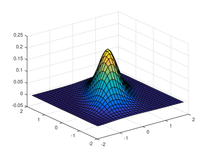
Figure 1: The estimated 3-dimensional joint density of a max-stable process using our algorithm

We calculate the $95\%$ confidence interval of the density on several selected values of the process $M(\cdot)$.

Values ($x$)	(0,0,0)	(0,0.5,0)	(0.5,0,0)	(0,-0.5,0)	(-0.5,0,0)
est. density ${\hat{f}}_{b}{(x)}$	0.2126	0.106	0.1292	0.1039	0.1439
lower CI	0.1916	0.0971	0.1180	0.0947	0.1311
upper CI	0.2336	0.1149	0.14036	0.1131	0.1567
Relative error	5.05%	4.29%	4.41%	4.54%	4.53%

As a comparison, we also calculate the $95\%$ confidence interval of the density using the plug-in kernel density estimation (KDE) method with the same amount ($b=10^{6}$) of i.i.d. samples of $M$. We use the normal density function as the kernel function and select the bandwidth according to [14]. The estimator is obtained as follows. Sample $M^{(1)},M^{(2)},\ldots,M^{(d)}$ i.i.d. copies of $M$, let $h_{b}=b^{-1/(2d+1)}$ and compute the sample covariance matrix, $\hat{\Sigma}$, based on $(M^{(1)},M^{(2)},\ldots,M^{(d)})$. Then, let

$$\hat{f}_{b}^{KDE}(x)=\frac{1}{bh_{b}^{d}}\sum_{i=1}^{b}\phi\left(A^{-\frac{1}{2}}\frac{x-M^{\left(i\right)}}{h_{b}}\right),$$

where $A=\hat{\Sigma}/$det$|\hat{\Sigma}|$. We apply the method from [4] to evaluate the corresponding confidence interval, thereby obtaining the following estimates,

Values ($x$)	(0,0,0)	(0,0.5,0)	(0.5,0,0)	(0,-0.5,0)	(-0.5,0,0)
est. density $\hat{f}_{b}^{KDE}(x)$	0.2163	0.0846	0.1143	0.0938	0.1084
lower CI	0.1953	0.0712	0.0999	0.0800	0.0934
upper CI	0.2373	0.0980	0.1287	0.1076	0.1234
Relative error	4.94%	8.07%	6.43%	7.51%	7.05%

From the above tables, we can see that our algorithm provides similar estimates to those obtained using the KDE. However, our estimator also has a smaller relative error when the estimated value is relatively small. Also, as discussed in [4], one must carefully choose the bandwidth to guarantee coverage because the KDE may be asymptotically biased. In contrast, the construction of confidence intervals with our estimator is a straightforward application of elementary statistical tools.

5 Appendix: A Detailed Algorithmic Implementation

In order to make this paper as self-contained as possible, we reproduce here the algorithms from [8] which allow us to simulate the random variables $N_{X}$, $N_{A}$, and $N_{a}$, jointly with $(A_{n})_{n\leq N}$ and $(X_{n})_{n\leq N}$.

5.1 Simulating Last Passage Times of Random Walks

Define the random walk $S_{n}=\gamma n-A_{n}$ for $n\geq 0$. Note that $ES_{n}<0$, by our choice of $\gamma<E\left(A_{1}\right)$. The authors in [8], argue that the choice of $\gamma$ is not too consequential so we shall assume that $\gamma=1/2$.

Here we review an algorithm from [8] for finding a random time $N_{S}$ such that $S_{n}<0$ for all $n>N_{S}$. Observe that $N_{S}=N_{A}$.

The algorithm is based on alternately sampling upcrossings and downcrossings of the level $0$. We write $\xi_{0}^{+}=0$ and, for $i\geq 1$, we recursively define

$$\xi_{i}^{-}=\begin{cases}\inf\{n\geq\xi_{i-1}^{+}:S_{n}<0\}&\text{if }\xi_{i-1}^{+}<\infty\\ \infty&\text{otherwise}\end{cases}$$

together with

$$\xi_{i}^{+}=\begin{cases}\inf\{n\geq\xi_{i}^{-}:S_{n}\geq 0\}&\text{if }\xi_{i}^{-}<\infty\\ \infty&\text{otherwise}.\end{cases}$$

As usual, in these definitions, the infimum of an empty set should be interpreted as $\infty$. Writing

$$N_{S}=\sup\{\xi_{n}^{-}:\xi_{n}^{-}<\infty\},$$

we have by construction $S_{n}<0$ for $n>N_{S}$. The random variable $N_{S}-1$ is an upward last passage time:

$$N_{S}-1=\sup\{n\geq 0:S_{n}\geq 0\}.$$

Note that $0\leq N_{S}<\infty$ almost surely under $P$ since $(S_{n})_{n\geq 0}$ starts at the origin and has negative drift. We will provide pseudo-codes for simulating $(S_{1},\ldots,S_{N_{S}+\ell})$ for any fixed $\ell\geq 0$, but first we need a few definitions.

First, we assume that the Cramér’s root, $\theta>0$, satisfying $E(\exp(\theta S_{1}))=1$ has been computed. We shall use $\mathbb{P}_{x}$ to denote the measure under which $\left(A_{n}\right)_{n\geq 1}$ are arrivals of a Poisson process with unit rate and $S_{0}=x$. Then, we define $P_{x}^{\theta}$ through an exponential change of measure. In particular, on the $\sigma$-field generated by $S_{1},\ldots,S_{n}$ we have

$$\frac{dP_{x}}{dP_{x}^{\theta}}=\exp(-\theta(S_{n}-x)).$$

It turns out that under $P_{x}^{\theta}$, $\left(A_{n}\right)_{n\geq 1}$ corresponds to the arrivals of a Poisson process with rate $1-\theta$ and the random walk $(S_{n})_{n\geq 1}$ has a positive drift.

To introduce the algorithm to sample $(S_{1},\ldots,S_{N_{S}+\ell})$ we first need the following definitions:

$$\tau^{-}=\inf\{n\geq 0:S_{n}<0\},\quad\quad\tau^{+}=\inf\{n\geq 0:S_{n}\geq 0\}.$$

For $x\geq 0$, it is immediate that we can sample a downcrossing segment $S_{1},\ldots,S_{\tau^{-}}$ under $P_{x}$ due to the negative drift, and we record this for later use in a pseudocode function. Throughout our discussion,‘sample’ in pseudocode stands for ‘sample independently of anything that has been sampled already’.

Function SampleDowncrossing($x$): Samples $(S_{1},\ldots,S_{\tau^{-}})$ under $P_{x}$ for $x\geq 0$

Step 1:  Return sample $S_{1},\ldots,S_{\tau^{-}}$ under $P_{x}$.

Step 2: EndFunction

Sampling an upcrossing segment is more interesting because it is possible that $\tau^{+}=\infty$. So, an algorithm needs to be able to detect this event within a finite amount of computing resources. For this reason, we understand sampling an upcrossing segment under $P_{x}$ for $x<0$ to mean that an algorithm outputs $S_{1},\ldots,S_{\tau^{+}}$ if $\tau^{+}<\infty$, and otherwise it outputs ‘degenerate’. The following pseudo-code samples an upcrossing under $P_{x}$ for $x<0$.

Function SampleUpcrossing($x$): Samples $(S_{1},\ldots,S_{\tau^{+}})$ under $P_{x}$ for $x<0$

Step 1: $S\leftarrow$ sample $S_{1},\ldots,S_{\tau^{+}}$ under $P_{x}^{\theta}$

Step 2: $U\leftarrow$ sample a standard uniform random variable

Step 3: If $U\leq\exp(-\theta(S_{\tau^{+}}-x))$

Step 4:  Return $S$

Step 5: Else

Step 6:  Return ‘degenerate’

Step 7: EndIf

Step 8: EndFunction

We next describe how to sample $(S_{k})_{k=1,\ldots,n}$ from $P_{x}$ conditionally on $\tau^{+}=\infty$ for $x<0$. Since $\tau^{+}=\infty$ is equivalent to $\sup_{k\leq\ell}S_{k}<0$ and $\sup_{k>\ell}S_{k}<0$ for any $\ell\geq 1$, after sampling $S_{1},\ldots,S_{\ell}$, by the Markov property we can use SampleUpcrossing$(S_{\ell})$ to verify whether or not $\sup_{k>\ell}S_{k}<0$.

Function SampleWithoutRecordS$\left({x,\ell}\right)$: Samples $(S_{k})_{k=1,\ldots,\ell}$ from $P_{x}$ given $\tau^{+}=\infty$ for $\ell\geq 1$, $x<0$

Step 1: Repeat

Step 2:$\qquad S\leftarrow$ sample $(S_{k})_{k=1,\ldots,\ell}$ under $P_{x}$

Step 3: Until $\sup_{1\leq k\leq\ell}S_{k}<0$ and SampleUpcrossing$(S_{\ell})$ is ‘degenerate’

Step 4: Return $S$

Step 5: EndFunction

We summarize our discussion with the full algorithm for sampling $(S_{0},\ldots,S_{N_{S}+\ell})$ under $P$ given some $\ell\geq 0$.

Algorithm S: Samples $S=(S_{0},\ldots,S_{N_{S}+\ell})$ under $P$ for $\ell\geq 0$

# We use $S_{\text{end}}$ to denote the last element of $S$.

Step 1: $S\leftarrow[0]$

Step 2:  Repeat

Step 3:  DowncrossingSegment $\leftarrow$ SampleDowncrossing$(S_{\text{end}})$

Step 4:$\qquad S\leftarrow[S,$Do$\text{wncrossingSegment}]$

Step 5:  UpcrossingSegment $\leftarrow$SampleUpcrossing$(S_{\text{end}})$

Step 6:  If UpcrossingSegment is not ‘degenerate’

Step 7:$\qquad\qquad S\leftarrow[S,\text{upcrossingSegment}]$

Step 8:   EndIf

Step 9:   Until UpcrossingSegment is ‘degenerate’

Step 10: If $\ell>0$

Step 11: $\qquad S\leftarrow[S,$SampleWithoutRecordS$(S_{\text{end}},\ell)]$

Step 12: EndIf

5.2 Simulating Last Passage Times for Maxima of Gaussian Vectors

The technique is similar to the random walk case using a sequence of record-breaking times. The parameter $a\in\left(0,1\right)$ can be chosen arbitrarily, but [8] suggests selecting $a$ such that

$$\exp\left(\frac{\overline{\sigma}}{a}\overline{\Phi}^{-1}\left(\delta\sqrt{2\pi}{\frac{\phi(\overline{\sigma}/a)}{d\overline{\sigma}/a}}\right)+\frac{\overline{\sigma}^{2}}{a^{2}}\right)=E\left[\left(\frac{A_{1}\,\exp(\left\|X\right\|_{\infty})}{\gamma}\right)^{\frac{1}{1-a}}\right],$$

where $\Phi(\cdot)$ is the cumulative distribution function of a standard Gaussian random variable and $\overline{\Phi}=1-\Phi$.

Now, assume that $\eta_{0}\geq 0$ is given (we will choose it specifically in the sequel). Let $(X_{n})_{n\geq 1}$ be i.i.d. copies of $X$ and define, for $i\geq 1$, a sequence of record breaking times $(\eta_{i})$ through

$$\eta_{i}=\begin{cases}\inf\{n>\eta_{i-1}:\left\|X_{n}\right\|_{\infty}>a\log n\}&\text{if }\eta_{i-1}<\infty\\ \infty&\text{otherwise.}\end{cases}.$$

We provide pseudo-codes which ultimately will allow us to sample $(X_{1},\ldots,X_{N_{X}+\ell})$ for any fixed $\ell\geq 0$, where

$$N_{X}=\max\{\eta_{i}:\eta_{i}<\infty\}.$$

First, we shall discuss how to sample $(X_{n})$ up to a $\eta_{1}$. In order to sample $\eta_{1}$, $\eta_{0}=n_{0}$ needs to be chosen so that $P(\left\|X\right\|_{\infty}>a\log n)$ is controlled for every $n>n_{0}$. Given the choice of $a\in\left(0,1\right)$, select $n_{0}$ such that

$${d\overline{\Phi}\left(\frac{a\log n_{0}}{\overline{\sigma}}-\frac{\overline{\sigma}}{a}\right)}\leq\frac{1}{2}\sqrt{\frac{\pi}{2}}{\frac{\phi(\overline{\sigma}/a)}{\overline{\sigma}/a}}.$$

Define

$$T_{n_{0}}=\inf\{k\geq 1:\left\|X_{k}\right\|_{\infty}>a\log(n_{0}+k)\}.$$ (24)

We describe an algorithm that outputs ‘degenerate’ if $T_{n_{0}}=\infty$ and $(X_{1},\ldots,X_{T_{n_{0}}})$ if $T_{n_{0}}<\infty$.

First, we describe a simple algorithm to simulate from $X$ conditioned on $\left\|X\right\|_{\infty}>a\log n$. Our algorithm makes use of a probability measure $P^{(n)}$ defined through

$$\frac{dP^{(n)}}{dP}(x)=\frac{\sum_{i=1}^{d}\mathbf{1}(\left|x(t_{i})\right|>a\,\log n)}{\sum_{i=1}^{d}{P(}\left|{X(t_{i})}\right|{>a\,\log n)}}.$$

It turns out that the measure $P^{(n)}$ approximates the conditional distribution of $X$ given that $\left\|X\right\|_{\infty}>a\log n$ for $n$ large.

Now, define $w^{j}(t)=\mathrm{Cov}(X(t),X(t_{j}))/\mathrm{Var}\left(X\left(t_{j}\right)\right)$ and note that $X\left(\cdot\right)-w^{\nu}\left(\cdot\right)X(t_{\nu})$ is independent of $X(t_{\nu})$ given $\nu$. This property is used in [8] to show that the following algorithm outputs from $P^{(n)}$. We will let $U$ be a uniform random variable in $\left(0,1\right)$ and $J$ is independent of $U$ and such that $P\left(J=1\right)=1/2=P\left(J=-1\right)$.)

Function ConditionedSampleX $\left(a,n\right)$: Samples $X$ from $P^{(n)}$

Step 1: $\nu\leftarrow$ sample with probability mass function

$$P(\nu=j)=\frac{P(\left|X(t_{j})\right|>a\log n)}{\sum_{i=1}^{d}{P(}\left|{X(t_{i})}\right|{>a\log n)}}$$

Step 2: $U\leftarrow$ sample a standard uniform random variable

Step 3: $X(t_{\nu})\leftarrow\sigma(t_{\nu})\cdot J\cdot\Phi^{-1}\left(U+(1-U)\Phi\left(a\left(\log n\right)/\sigma(t_{\nu})\right)\right)$ # Conditions on $\left|X(t_{\nu})\right|>a\log n$

Step 4: $Y\leftarrow$ sample of $X$ under $P$

Step 5: Return $Y(t)-w^{\nu}(t)Y(t_{\nu})+X(t_{\nu})$

Step 6: EndFunction

We now explain how ConditionedSampleX is used to sample $T_{n_{0}}$. Define, for $k\geq 1$,

$$g_{n_{0}}(k)=\frac{\int_{k-1}^{k}\phi((a\log(n_{0}+s))/\overline{\sigma})ds}{\int_{0}^{\infty}\phi((a\log(n_{0}+s))/\overline{\sigma})ds},$$

where $\phi(x)=d\Phi(x)/dx$. Note that $g_{n_{0}}(\cdot)\geq 0$ defines the probability mass function of some random variable $K$. It turns out that if $U\sim U\left(0,1\right)$ then we can sample

$$K=\left\lceil\exp\left\{\frac{\overline{\sigma}^{2}}{a^{2}}+\frac{\overline{\sigma}}{a}\overline{\Phi}^{-1}\left(U\,\overline{\Phi}\left(\frac{a\log n_{0}}{\overline{\sigma}}-\frac{\overline{\sigma}}{a}\right)\right)\right\}-n_{0}\right\rceil.$$

The next function samples $(X_{1},\ldots,X_{T_{n_{1}}})$ for $n_{1}\geq n_{0}$.

Function SampleSingleRecord $\left(a,n_{0},n_{1}\right)$: Samples $(X_{1},\ldots,X_{T_{n_{1}}})$ for $a\in(0,1),n_{1}\geq n_{0}\geq 0$

Step 1: Sample $K$

Step 2: $[X_{1},\ldots,X_{K-1}]\leftarrow$ i.i.d. sample from $P$

Step 3: $X_{K}$ $\leftarrow\text{ {ConditionedSampleX}}(a,n_{1}+K)$

Step 4: $U\leftarrow$ sample a standard uniform random variable

Step 5: If $\left\|{X_{k}}\right\|_{\infty}$$\leq a\log(n_{1}+k)$ for $k=1,\ldots,K-1$ and $U\,{g_{n_{0}}(K)}\leq{dP/dP^{(n_{1}+K)}(X_{K})}$

Step 6:   Return $(X_{1},\ldots,X_{K})$

Step 7: Else

Step 8:   Return ‘degenerate’

Step 9: EndIf

Step 10: EndFunction

We next describe how to sample $(X_{k})_{k=1,\ldots,n}$ conditionally on $T_{n_{0}}=\infty$. This is a simple task because the $X_{n}$s are independent.

Function SampleWithoutRecordX $\left(n_{1},\ell\right)$ : Samples $(X_{k})_{k=1,\ldots,\ell}$ conditionally on $T_{n_{1}}=\infty$ for $\ell\geq 1$

Step 1: Repeat

Step 2:   $X\leftarrow$ sample $(X_{k})_{k=1,\ldots,\ell}$ under $P$

Step 3: Until $\sup_{1\leq k\leq\ell}[X_{k}-a\log(n_{1}+k)]<0$

Step 4: Return $X$

Step 5: EndFunction

We now can explain how to sample $(X_{1},\ldots,X_{N_{X}+\ell})$ under $P$ given some $\ell\geq 0$. The idea is to successively apply SampleSingleRecord to generate the sequence $\left(\eta_{i}:i\geq 1\right)$ defined at the beginning of this section. Starting from $\eta_{0}=n_{0}$, then $n_{1}$ is replaced by each of the subsequent $\eta_{i}$s.

Algorithm X: Samples $(X_{1},\ldots,X_{N_{X}+\ell})$ given $a\in(0,1)$, $\overline{\sigma}>0$, $\ell\geq 0$

Step 1: $X\leftarrow[\,]$, $\eta\leftarrow n_{0}$

Step 2: $X\leftarrow$ sample $(X_{k})_{k=1,\ldots,\eta}$ under $P$

Step 3: Repeat

Step 4:   segment $\leftarrow\text{ {SampleSingleRecord}}(a,n_{0},\eta)$

Step 5:   If segment is not ‘degenerate’

Step 6:     $X\leftarrow[X,\text{segment}]$

Step 7:     $\eta\leftarrow\text{length}(X)$

Step 8:   EndIf

Step 9: Until segment is ‘degenerate’

Step 10: If $\ell>0$

Step 11:   $X\leftarrow[X,\text{{SampleWithoutRecordX}}(\eta,\ell)]$

Step 12: EndIf

5.3 Algorithm to Sample $X_{1},...,X_{N},N$

The final algorithm for sampling $M,X_{1},...,X_{N},N$ is given next.

Algorithm M: Samples $M,X_{1},...,X_{N},N$ given $a\in(0,1)$, $\gamma<E\left(A_{1}\right)$, and $\overline{\sigma}$

Step 1: Sample $A_{1},\ldots,A_{N_{A}}$ using Steps 1–9 from Algorithm S with $S_{n}=\gamma n-A_{n}$.

Step 2: Sample $X_{1},\ldots,X_{N_{X}}$ using Steps 1–9 from Algorithm X.

Step 3: Calculate $N_{a}$ with (9) and set $N=\max(N_{A},N_{X},N_{a})$.

Step 4: If $N>N_{A}$

Step 5:   Sample $A_{N_{A}+1},\ldots,A_{N}$ as in Step 10–12 from Algorithm S with $S_{n}=\gamma n-A_{n}$.

Step 6: EndIf

Step 7: If $N>N_{X}$

Step 8:   Sample $X_{N_{X}+1},\ldots,X_{N}$ as in Step 10–12 from Algorithm X.

Step 9: EndIf

Step 10: Return $M(t_{i})=\max_{1\leq n\leq N}\left\{-\log A_{n}+X_{n}(t_{i})+\mu(t_{i})\right\}$ for $i=1,\ldots,d$, and $X_{1},...,X_{N},N$.

References

• [1] J. H. Blanchet and Z. Liu. Efficient Conditional Density Estimation for Max-Stable Fields. Submitted.
• [2] P. Embrechts, C. Klüppelberg, and T. Mikosch. Modelling Extremal Events for Insurance and Finance. Springer, New York, 1997.
• [3] L. C. Evans. Partial Differential Equations: Second Edition. American Mathematical Society, 2010.
• [4] C. V. Fiorio. Confidence intervals for kernel density estimation. Stata Journal, 4:168–179, 2004.
• [5] M. B. Giles. Multilevel Monte Carlo path simulation. Operations Research, 56(3):607–617, 2008.
• [6] R. Huser and A. C. Davison. Composite likelihood estimation for the Brown-Resnick process. Biometrika, 100(2):511-518, 2013.
• [7] A. Kohatsu-Higa and K. Yasuda. Estimating Multidimensional Density Functions Using the Malliavin-Thalmaier Formula. SIAM Journal on Numerical Analysis, 47:1546–1575, 2009.
• [8] Z. Liu, J. H. Blanchet, A. B. Dieker, and T. Mikosch. Optimal exact simulation of max-stable and related random fields. Submitted. Preprint arXiv:1609.06001.
• [9] P. Malliavin and A. Thalmaier. Stochastic Calculus of Variations in Mathematical Finance. Springer, New York, 2006.
• [10] D. McLeish. A general method for debiasing a Monte Carlo estimator. Monte Carlo Methods and Applications, 17(4), 2011.
• [11] C. H. Rhee and P. W. Glynn. Unbiased estimation with square root convergence for SDE Models. Operations Research, 63(5):1026–1043, 2015.
• [12] M. Ribatet. Spatial extremes: max-stable processes at work. Journal de La Société Frana̧ise de Statistique, 154(2):156–177, 2013.
• [13] C. Y. Robert and J. Segers. Tails of random sums of a heavy-tailed number of light-tailed terms. Insurance: Mathematics and Economics, 43(1):85–92, 2008.
• [14] D. W. Scott and S. R. Sain. Multidimensional density estimation. Handbook of Statistics, 24:229–261, 2005.
• [15] Z. Zheng, J. Blanchet, and P. W. Glynn. Rates of convergence and CLTs for subcanonical debiased MLMC. Submitted.