Analysis and Control of Stochastic Systems using Semidefinite Programming over Moments

Abstract

This paper develops a unified methodology for probabilistic analysis and optimal control design for jump diffusion processes defined by polynomials. For such systems, the evolution of the moments of the state can be described via a system of linear ordinary differential equations. Typically, however, the moments are not closed and an infinite system of equations is required to compute statistical moments exactly. Existing methods for stochastic analysis, known as closure methods, focus on approximating this infinite system of equations with a finite dimensional system. This work develops an alternative approach in which the higher order terms, which are approximated in closure methods, are viewed as inputs to a finite-dimensional linear control system. Under this interpretation, upper and lower bounds of statistical moments can be computed via convex linear optimal control problems with semidefinite constraints. For analysis of steady-state distributions, this optimal control problem reduces to a static semidefinite program. These same optimization problems extend automatically to stochastic optimal control problems. For minimization problems, the methodology leads to guaranteed lower bounds on the true optimal value. Furthermore, we show how an approximate optimal control strategy can be constructed from the solution of the semidefinite program. The results are illustrated using numerous examples.

I Introduction

Stochastic dynamics and stochastic optimal control problems arise in a variety of domains such as finance [1, 2, 3, 4], biology [5, 4], physics [5], robotics [6], probabilistic inference [7, 8], and stochastic approximation algorithms [9]. In stochastic analysis problems, statistics such as the average size of a biological population [10, 11] or the average density of a gas [12] are desired. Aside from special stochastic processes, such as linear Gaussian systems, these statistics can rarely be computed analytically. Typically, estimates of the statistics are either found through Monte Carlo simulation or approximation schemes. In stochastic optimal control, a controller attempts to achieve a desired behavior in spite of noise. For example, a robot must make reaching movements in the face of noisy actuation [6], or the harvest of a fishery must be managed despite random fluctuations in the fish supply [13, 14]. Aside from linear systems with quadratic costs, few stochastic optimal control problems can be solved analytically.

I-A Contribution

This paper defines a unified methodology for approximating both analysis and control problems via convex optimization methods. The paper focuses on continuous-time jump diffusions defined by polynomials. Both finite-horizon and steady-state problems are considered. In the finite-horizon case, approximations are achieved by solving an auxiliary linear optimal control problem with semidefinite constraints. In the steady-state case, this problem reduces to a static semidefinite program (SDP).

In the case of stochastic analysis problems, our method can be used to provide provable upper and lower bounds on statistical quantities of interest. For analysis problems, the method can be viewed as an alternative to moment closure methods [15, 12, 10, 16, 17, 18], which give point approximations to moments, as opposed to bounds.

For stochastic optimal control problems, the auxiliary optimal control problem is a convex relaxation of the original problem. In the case of stochastic minimization problems, the relaxation gives provable lower bounds on the true optimal value. Furthermore, we provide a method for constructing feasible controllers for the original system. The lower bound from the relaxation can then be used to compute the optimality gap of the controller.

This work is an extension of the conference paper [19]. That paper only considered the case of finite-horizon optimal control for stochastic differential equations. The current work considers both finite-horizon and steady-state problems. Additionally, the methods are extended to include jump processes. Furthermore, this paper treats stochastic analysis and stochastic control problems in a unified manner.

I-B Related Work

For uncontrolled problems, the work is closely related to the moment closure problems discussed briefly above. The moment closure problem arises when dynamics of one moment depend on higher order moments, and so moments of interest cannot be represented by a finite collection of equations. Moment closure methods utilize probabilistic or physical principles to replace higher order moments with approximate values. This work, in contrast, uses the higher order moments as inputs to an auxiliary linear optimal control problem. A special case of this idea corresponding to stationary moments of stochastic differential equations was independently studied in [20].

Most methods for stochastic optimal control focus on dynamic programming [21, 22] or approximate dynamic programming [23]. More closely related to this work, however, are relaxation methods. Unlike approximate dynamic programming, these methods provide bounds on the achievable optimal values. The most closely related methods focus on occupation measures [24, 25, 26]. These works rely on the general insight that a convex relaxation of an optimization problem can be obtained by examining randomized strategies [27]. Such relaxation methods apply to stochastic optimal control problems, but it is not clear that they can be used for analysis problems. In contrast, our relaxation methodology applies to both cases. A more removed relaxation method is studied in [28, 29]. These works use duality to relax the constraint that controllers depend causally on state information. Also related is the work of [30, 31] which uses a combination of moment dynamics and deterministic optimal control to find approximate solutions to stochastic optimal control problems. This work, however, only considers systems with closed moments. Furthermore, this work assumes a fixed parametric form for the controller, and does not obtain a relaxation of the original stochastic control problem.

I-C Paper Organization

Section II defines the general problems of interest. In this section, a collection of running examples is also introduced. Background results on stochastic processes are given in Section III. The main results along with numerical examples are given in Section IV. Finally, the conclusions are given in Section V.

II Problems

This paper develops a methodology for bounding the moments of stochastic dynamical systems and stochastic control problems in continuous-time. This section introduces the classes of problems for which we can apply our new technique. Subsection II-B describes the uncontrolled stochastic systems, Subsection II-C describes the optimal stochastic control problems, and Subsection II-D describes the steady state variants of these problems. Throughout the section, we will introduce running examples that illustrate how each of the problems specializes to concrete systems.

II-A Notation

Random variables are denoted in bold.

If $\boldsymbol{x}$ and $\boldsymbol{y}$ are identically distributed random variables, we denote this by $\boldsymbol{x}\stackrel{{\scriptstyle d}}{{=}}\boldsymbol{y}$.

For a stochastic process, $\boldsymbol{x}(t)$, $d\boldsymbol{x}(t)$ denotes the increment $\boldsymbol{x}(t+dt)-\boldsymbol{x}(t)$.

If $\boldsymbol{x}$ is a random variable, its expectation is denoted by $\langle\boldsymbol{x}\rangle$.

We denote that $\boldsymbol{x}$ is a Gaussian random variable with mean $\mu$ and covariance $\Sigma$ by $\boldsymbol{x}\sim\mathcal{N}(\mu,\Sigma)$. More generally, we write $\boldsymbol{x}\sim\mathcal{D}$ to denote that $\boldsymbol{x}$ is distributed according to some distribution $\mathcal{D}$.

The notation $M\succeq 0$ denotes that $M$ is a symmetric, positive semidefinite matrix. If $v$ is a vector, then $v\geq 0$ indicates that all elements of $v$ are non-negative.

The set of non-negative integers is denoted by $\mathbb{N}$.

II-B Bounding Moments of Stochastic Dynamic Systems

In this subsection, we pose the problem of providing bounds to moments of stochastic processes. The processes take the form of continuous-time jump diffusions with non-homogeneous jump rates:

$$d\boldsymbol{x}(t)=f(\boldsymbol{x}(t))dt+g(\boldsymbol{x}(t))d\boldsymbol{w}(t)+\sum_{i=1}^{J}(\phi_{i}(\boldsymbol{x}(t))-\boldsymbol{x}(t))d\boldsymbol{N}_{i}(\boldsymbol{x}(t)).$$ (1)

Here $\boldsymbol{x}(t)$ is the state and $\boldsymbol{w}(t)$ is a Brownian motion with $\boldsymbol{w}(t)\sim\mathcal{N}(0,tI)$. The terms $d\boldsymbol{N}_{i}(\boldsymbol{x}(t))$ are increments of independent non-homogeneous Poisson process with jump intensity $\lambda_{i}(\boldsymbol{x}(t))$, so that

$$d\boldsymbol{N}_{i}(\boldsymbol{x}(t))=\begin{cases}1&\textrm{ with probability }\lambda_{i}(\boldsymbol{x}(t))dt\\ 0&\textrm{ with probability }1-\lambda_{i}(\boldsymbol{x}(t))dt.\end{cases}$$ (2)

It will be assumed that the initial condition is either a constant, $\boldsymbol{x}(0)=x_{0}$, or that $\boldsymbol{x}(0)$ is a random variable with known moments.

We assume that all of the functions, $f$, $g$, $\phi_{i}$ and $\lambda_{i}$, are polynomials. Let $c$ and $h$ be polynomial functions.

Remark 1

Recall that $d\boldsymbol{x}(t)=\boldsymbol{x}(t+dt)-\boldsymbol{x}(t)$ and $d\boldsymbol{w}(t)\sim\mathcal{N}(0,dtI)$. Thus, the equations (1) and (2) can be used to simulate the system using an Euler-Maruyama method. However, as written, the equations do not uniquely specify the behavior of the Poisson processes. In particular, over the interval $[t,t+dt]$, more than one of the processes may have a jump. In this scenario, it is not clear which of the jumps occurs first. This ambiguity can be resolved by instead simulating the following identically distributed jump process:

$$\sum_{i=1}^{J}\left(\phi_{i}(\boldsymbol{x}(t))-\boldsymbol{x}(t)\right)d\boldsymbol{N}_{i}(\boldsymbol{x}(t)) \stackrel{{\scriptstyle d}}{{=}}\boldsymbol{z}(t)d\boldsymbol{N}(\boldsymbol{x}(t))$$ (3a)

$$d\boldsymbol{N}(\boldsymbol{x}(t)) =\begin{cases}1&\textrm{ with probability }\sum_{i=1}^{J}\lambda_{i}(\boldsymbol{x}(t))dt\\ 0&\textrm{ with probability }1-\sum_{i=1}^{J}\lambda_{i}(\boldsymbol{x}(t))dt\end{cases}$$ (3b)

$$\boldsymbol{z}(t) =\phi_{j}(\boldsymbol{x}(t))-\boldsymbol{x}(t)\quad\textrm{with probability}\quad\frac{\lambda_{j}(\boldsymbol{x}(t))}{\sum_{i=1}^{J}\lambda_{i}(\boldsymbol{x}(t))}.$$ (3c)

We assume that there is some quantity of interest that can be described by

$$\left\langle\int_{0}^{T}c(\boldsymbol{x}(t))dt+h(\boldsymbol{x}(T))\right\rangle,$$ (4)

where $c$ and $h$ are polynomials. Such a quantity could represent, for example, total energy expenditure over an interval, or variance of the state at the final time.

Our first problem, solved in Subsection IV-A, is to give a systematic method for computing an increasing sequence of lower bounds, $\mathfrak{L}_{i}$ and a decreasing sequence of upper bounds $\mathfrak{U}_{i}$ that satisfy:

$$\mathfrak{L}_{0}\leq\cdots\leq\mathfrak{L}_{i}\leq\left\langle\int_{0}^{T}c(\boldsymbol{x}(t))dt+h(\boldsymbol{x}(T))\right\rangle\leq\mathfrak{U}_{i}\leq\cdots\leq\mathfrak{U}_{0}.$$ (5)

Below we will give a few running examples of systems defined by (1), (2) and (4).

Example 1 (Stochastic Logistic Model)

Consider the stochastic logistic model studied in [11]. This model is described by:

$$\boldsymbol{x}(t+dt)=\begin{cases}\boldsymbol{x}(t)+1&\textrm{ with probability }\lambda_{1}(\boldsymbol{x}(t))dt\\ \boldsymbol{x}(t)-1&\textrm{ with probability }\lambda_{2}(\boldsymbol{x}(t))dt\\ \boldsymbol{x}(t)&\textrm{ otherwise},\end{cases}$$ (6)

where the jump intensities are given by:

$$\lambda_{1}(x)=a_{1}x-b_{1}x^{2},\qquad\lambda_{2}(x)=a_{2}x+b_{2}x^{2}.$$ (7)

Here we assume that the coefficients satisfy:

$$\Omega:=\frac{a_{1}}{b_{1}}\in\mathbb{N},\quad a_{1}>0,\quad a_{2}>0,\quad b_{1}>0,\quad b_{2}\geq 0.$$ (8)

These assumptions guarantee that if $\boldsymbol{x}(0)\in\{0,1,2,\ldots,\Omega\}$ then $\boldsymbol{x}(t)\in\{0,1,2,\ldots,\Omega\}$ for all $t\geq 0$. We will analyze the moments of this system via semidefinite programming (SDP). We will see that the bounds on the process can be incorporated as constraints in the SDP.

This system is a special case of (1) with $f=0$, $g=0$, $\phi_{1}(x)=x+1$, $\phi_{2}(x)=x-1$, and $\lambda_{i}$ defined as above.

II-C Stochastic Optimal Control

For optimal control, the systems are similar, except now in addition to the state process, $\boldsymbol{x}(t)$, there is also an input process, $\boldsymbol{u}(t)$.

The general problem has the form:

minimize $$\left\langle\int_{0}^{T}c(\boldsymbol{x}(t),\boldsymbol{u}(t))dt+h(\boldsymbol{x}(T),\boldsymbol{u}(T))\right\rangle$$ (9a)

subject to $$d\boldsymbol{x}(t)=f(\boldsymbol{x}(t),\boldsymbol{u}(t))dt+g(\boldsymbol{x}(t),\boldsymbol{u}(t))d\boldsymbol{w}(t)+\sum_{i=1}^{J}\left(\phi_{i}(\boldsymbol{x}(t),\boldsymbol{u}(t))-\boldsymbol{x}(t)\right)d\boldsymbol{N}_{i}(\boldsymbol{x}(t),\boldsymbol{u}(t))$$ (9b)

$$d\boldsymbol{N}_{i}(\boldsymbol{x}(t),\boldsymbol{u}(t))=\begin{cases}1&\textrm{ with probability }\lambda_{i}(\boldsymbol{x}(t),\boldsymbol{u}(t))dt\\ 0&\textrm{ with probability }1-\lambda_{i}(\boldsymbol{x}(t),\boldsymbol{u}(t))dt\end{cases}$$ (9c)

$$b_{i}(\boldsymbol{x}(t),\boldsymbol{u}(t))\geq 0\quad\textrm{for}\quad i\in\{1,\ldots,n_{b}\}$$ (9d)

$$\boldsymbol{x}(0)\sim\mathcal{D}$$ (9e)

$$\boldsymbol{u}(t)\textrm{ is admissible.}$$ (9f)

Here $\boldsymbol{x}(0)\sim\mathcal{D}$ means that $\boldsymbol{x}(0)$ has some specified initial distribution, $\mathcal{D}$. In the problems studied, $\mathcal{D}$ will either be a Dirac $\delta$ function, specifying a constant initial condition, or else $\mathcal{D}$ will be a distribution with known moments.

By admissible, we mean that $\boldsymbol{u}(t)$ is measurable with respect to the filtration $\mathcal{F}(t)$ generated by $\{\boldsymbol{x}(\tau):0\leq\tau\leq t\}$. As with the uncontrolled case, we assume that all of the systems are polynomial.

Let $V^{*}$ be the optimal cost. The method to be described in Subsection IV-A gives a semidefinite programming method for computing an increasing sequence of lower bounds, $\mathfrak{L}_{i}$ on the optimal cost:

$$\mathfrak{L}_{0}\leq\cdots\leq\mathfrak{L}_{i}\leq V^{*}.$$ (10)

In Subsection IV-C, we show how to use the result of the semidefinite programs to produce feasible controllers. The cost associated with any feasible controller will necessarily be at least as high as the optimal cost, and so the corrsponding controller gives an upper bound $\mathfrak{U}_{i}$. So, we must have that $\mathfrak{L}_{i}\leq V^{*}\leq\mathfrak{U}_{i}$. So, if this gap is small, then the controller must be nearly optimal.

Example 2 (LQR)

We present the linear quadratic regulator problem because it is well-known, and it fits into the general framework of our problem. Unlike most of the problems studied, all of the associated optimization problems can be solved analytically in this case.

minimize $$\left\langle\int_{0}^{T}\left(\boldsymbol{x}(t)^{\top}Q\boldsymbol{x}(t)+\boldsymbol{u}(t)^{\top}R\boldsymbol{u}(t)\right)dt\right\rangle+\left\langle\boldsymbol{x}(T)^{\top}\Psi\boldsymbol{x}(T)\right\rangle$$ (11a)

subject to $$d\boldsymbol{x}(t)=(\mathcal{A}\boldsymbol{x}(t)+\mathcal{B}\boldsymbol{u}(t))dt+\mathcal{G}d\boldsymbol{w}(t)$$ (11b)

$$\boldsymbol{x}(0)\sim\mathcal{N}(0,\Sigma).$$ (11c)

Here $\boldsymbol{x}(0)\sim\mathcal{N}(0,\Sigma)$ means that $\boldsymbol{x}(0)$ is a Gaussian random variable with mean zero and covariance $\Sigma$.

We examine this problem because the SDP from Subsection IV-A and the controller construction method from Subsection IV-C give exact solutions in this case. In other cases, they only provide lower and upper bounds, respectively.

Example 3 (Fishery Management)

Consider the modified version of the optimal fisheries management from [13, 14]:

maximize $$\left<\int_{0}^{T}\boldsymbol{u}(t)dt\right>$$ (12a)

subject to $$d\boldsymbol{x}(t)=\left(\boldsymbol{x}(t)-\gamma\boldsymbol{x}(t)^{2}-\boldsymbol{u}(t)\right)dt+\sigma\boldsymbol{x}(t)d\boldsymbol{w}(t)$$ (12b)

$$\boldsymbol{x}(0)=x_{0}$$ (12c)

$$\boldsymbol{x}(t)\geq 0$$ (12d)

$$\boldsymbol{u}(t)\geq 0.$$ (12e)

Here $\boldsymbol{x}(t)$ models the population in a fishery and $\boldsymbol{u}(t)$ models the rate of harvesting. As in the earlier works, a constraint that $\boldsymbol{x}(t)\geq 0$ is required to be physically meaningful. Also, without this constraint, the optimal strategy would be to set $\boldsymbol{u}(t)=+\infty$. The constraint that $\boldsymbol{u}(t)\geq 0$ encodes the idea that fish are only being taken out, not put into the fishery.

The primary difference between this formulation and that of [13] and [14], is that the cost is not discounted, and operates over a fixed, finite horizon.

Note that this is a maximization problem, but this is equivalent to minimizing the objective multiplied by $-1$.

Example 4 (Randomly Sampled Feedback)

Consider a system in which a state $\boldsymbol{x}_{1}(t)$ is controlled by a sampled feedback controller, where the sampling times are Poisson distributed. A simple version of this system is described below.

$$d\boldsymbol{x}_{1}(t) =\boldsymbol{x}_{2}(t)dt+d\boldsymbol{w}(t)$$ (13a)

$$x_{2}(t+dt) =\begin{cases}\boldsymbol{u}(t)&\textrm{ with probability }\lambda dt\\ \boldsymbol{x}_{2}(t)&\textrm{ with probability }1-\lambda dt.\end{cases}$$ (13b)

So, here the state $x_{2}(t)$ holds the most recent sample of the input $\boldsymbol{u}(t)$. A natural cost for this problem is of the form:

$$\left\langle\int_{0}^{T}\left(Q\boldsymbol{x}_{1}(t)^{2}+R\boldsymbol{x}_{2}(t)^{2}\right)dt\right\rangle.$$ (14)

II-D Steady State

Both the analysis problem and the control problem from Subsections II-B and II-C, respectively, deal with computing bounds on the moments of a stochastic process over a finite time horizon. The results for these problems can be modified in a straight-forward manner to bound steady-state moments of these problems. In this case, for example, the optimal control problem becomes:

minimize $$\lim_{T\to\infty}\left\langle h(\boldsymbol{x}(T),\boldsymbol{u}(T))\right\rangle$$ (15a)

subject to $$\eqref{eq:controlledDynamics}-\eqref{eq:controlledInequality}$$ (15b)

A special case of this problem was studied using similar methods in [20]. For a detailed discussion of the differences between those results and the present results, see Remark 6, below.

Example 5 (Jump Rate Control)

As another variation, we will consider the case of controlling the rate of jumps in a control system. A simple model of this takes the form:

$$\boldsymbol{x}(t+dt)=\begin{cases}\boldsymbol{x}(t)+d\boldsymbol{w}(t)&\textrm{ with probability }1-\boldsymbol{u}(t)dt\\ 0&\textrm{ with probability }\boldsymbol{u}(t)dt.\end{cases}$$ (16)

To get a well-posed optimal control problem, we will penalize a combination of $\boldsymbol{x}(t)$ and $\boldsymbol{u}(t)$, and further constrain $\boldsymbol{u}(t)$ to remain in a compact interval. The formal problem can be stated as a special case of (15):

minimize $$\lim_{T\to\infty}\left\langle Q\boldsymbol{x}(T)^{2}+R\boldsymbol{u}(T)\right\rangle$$ (17a)

subject to $$d\boldsymbol{x}(t)=d\boldsymbol{w}(t)-\boldsymbol{x}(t)d\boldsymbol{N}(t)$$ (17b)

$$d\boldsymbol{N}(t)=\begin{cases}1&\textrm{ with probability }\boldsymbol{u}(t)dt\\ 0&\textrm{ with probability }1-\boldsymbol{u}(t)dt\end{cases}$$ (17c)

$$0\leq\boldsymbol{u}(t)\leq\Omega.$$ (17d)

The constraint that $\boldsymbol{u}(t)\geq 0$ ensures that the jump rate is always non-negative. The upper bound constraint, $\boldsymbol{u}(t)\leq\Omega$ is more subtle, and is required to ensure finite jump rates. To see why it is required, note that the average-cost Hamilton-Jacobi-Bellman (HJB) equation for this problem is given by:

$$V^{*}=\min_{0\leq u\leq\Omega}\left[Qx^{2}+Ru+\frac{1}{2}\frac{\partial^{2}v(x)}{\partial x^{2}}+(v(0)-v(x))u\right].$$ (18)

Here $V^{*}$ is the optimal value of (17) and $v(x)$ is the differential cost-to-go function. Analysis of (18) shows that an optimal strategy must satisfy:

$$u=\begin{cases}0&\textrm{ if }R+v(0)-v(x)>0\\ \Omega&\textrm{ if }R+v(0)-v(x)<0.\end{cases}$$ (19)

If no upper bound on $u$ were given, then the optimal strategy would be to set $u=+\infty$ if $R+v(0)-v(x)<0$. This reduces to an event-triggered control strategy, [32, 33] in which an instantaneous jump occurs whenever the state crosses the boundary $R+v(0)-v(x)=0$. With the upper bound, the strategy approximates an event triggered strategy, but in this case, rather than an instantaneous jump, the jump rate goes as high as possible when the boundary is crossed. This ensures that a jump will occur with high probability.

It should be noted that while some general properties of the optimal strategy can be deduced by examining (18), solving this HJB equation appears to be non-trivial. First, it requires knowing the true optimal value $V^{*}$ and then solving a non-smooth partial differential equation for $v(x)$.

III Background Results

This section presents some basic results on expressing dynamics of moments using linear differential equations. Subsection III-A reviews well-known results on Itô’s formula and generators for jump processes. These results can be used to see how functions of a stochastic process evolve over time. Subsection III-B specializes the results from Subsection III-A to the problems studied in this paper, as defined in Section II. In particular, we will see that moments of the stochastic process are the solutions of an auxiliary linear control system. Furthermore, objectives and constraints on the original system can be encoded using linear mappings of the state and input of the auxiliary linear control system. Section III-C shows how the auxiliary linear control system and the corresponding linear mappings from Subsection III-B can be found in examples.

III-A Itô’s Formula and Generators

In this paper, we will examine the behavior of moments of a stochastic process. The dynamics of the moments can be derived using standard tools from stochastic processes. For more details, see [1, 4].

Consider the dynamics from (9b). Note that (1) is a special case of (9b) with all coefficients of $\boldsymbol{u}(t)$ set to zero. The Itô formula for jump processes implies that for any smooth scalar-valued function $h(\boldsymbol{x}(t))$, the increment is given by

$$dh(\boldsymbol{x}(t))=\frac{\partial h(\boldsymbol{x}(t))}{\partial x}\left(f(\boldsymbol{x}(t),\boldsymbol{u}(t))dt+g(\boldsymbol{x}(t),\boldsymbol{u}(t))d\boldsymbol{w}(t)\right)+\frac{1}{2}\mathrm{Tr}\left(\frac{\partial^{2}h(\boldsymbol{x}(t))}{\partial x^{2}}g(\boldsymbol{x}(t),\boldsymbol{u}(t))g(\boldsymbol{x}(t),\boldsymbol{u}(t))^{\top}\right)dt\\ +\sum_{i=1}^{J}\left(h(\phi_{i}(\boldsymbol{x}(t),\boldsymbol{u}(t)))-h(\boldsymbol{x}(t))\right)d\boldsymbol{N}_{i}(\boldsymbol{x}(t),\boldsymbol{u}(t)).$$ (20)

Taking expectations and dividing both sides by $dt$ gives the differential equation:

$$\frac{d}{dt}\langle h(\boldsymbol{x}(t))\rangle=\left\langle\frac{\partial h(\boldsymbol{x}(t))}{\partial x}f(\boldsymbol{x}(t),\boldsymbol{u}(t))+\frac{1}{2}\mathrm{Tr}\left(\frac{\partial^{2}h(\boldsymbol{x}(t))}{\partial x^{2}}g(\boldsymbol{x}(t),\boldsymbol{u}(t))g(\boldsymbol{x}(t),\boldsymbol{u}(t))^{\top}\right)\right\rangle\\ +\left\langle\sum_{i=1}^{J}\left(h(\phi_{i}(\boldsymbol{x}(t),\boldsymbol{u}(t)))-h(\boldsymbol{x}(t))\right)\lambda_{i}(\boldsymbol{x}(t),\boldsymbol{u}(t))\right\rangle.$$ (21)

The differential equation can be expressed compactly as $\frac{d}{dt}\langle h(\boldsymbol{x}(t))\rangle=\langle Lh(\boldsymbol{x}(t),\boldsymbol{u}(t))\rangle$, where $L$ is known as the generator of the jump process:

$$Lh(x,u)=\frac{\partial h(x)}{\partial x}f(x,u)+\frac{1}{2}\mathrm{Tr}\left(\frac{\partial^{2}h(x)}{\partial x^{2}}g(x,u)g(x,u)^{\top}\right)+\sum_{i=1}^{J}\left(h(\phi_{i}(x,u))-h(x)\right)\lambda_{i}(x,u).$$ (22)

Say that $h(\boldsymbol{x}(t))$ is a polynomial. Then, since all of the functions, $f$, $g$, $\phi_{i}$, and $\lambda_{i}$ are polynomials, term inside the expectation on the right hand side of (21) must also be a polynomial.

III-B The Auxiliary Linear System

This subsection specializes the results from the previous subsection to the problems defined in Section II. In particular, we will see how the dynamics, constraints, and costs can all be studied in terms of an auxiliary linear control system. It should be noted that the auxiliary control system has the same basic form regardless of whether the original system was an uncontrolled system, as introduced in Subsection II-B, or a stochastic optimal control problem, as introduced in Subsection II-C.

The state of our auxiliary control system $\mathcal{X}(t)$ will be a collection of moments:

$$\mathcal{X}(t)=\begin{bmatrix}1\\ \left\langle\boldsymbol{x}(t)^{(m_{1})}\right\rangle\\ \left\langle\boldsymbol{x}(t)^{(m_{2})}\right\rangle\\ \vdots\\ \left\langle\boldsymbol{x}(t)^{(m_{N})}\right\rangle\end{bmatrix}.$$ (23)

Here, we use the notation that if $m=(m_{1},m_{2},\ldots,m_{n})$, then $\boldsymbol{x}(t)^{(m)}$ denotes the product:

$$\boldsymbol{x}(t)^{(m)}=(\boldsymbol{x}_{1}(t))^{m_{1}}(\boldsymbol{x}_{2}(t))^{m_{2}}\cdots(\boldsymbol{x}_{n}(t))^{m_{n}}.$$ (24)

Note that $1=\left\langle\boldsymbol{x}(t)^{(0)}\right\rangle$, in $\mathcal{X}(t)$. For simplicity, $\mathcal{X}(t)$ will often include all moments of $\boldsymbol{x}(t)$ up to some degree.

The input to the auxiliary control system will be another collection of moments:

$$\mathcal{U}(t)=\begin{bmatrix}\left\langle\boldsymbol{x}(t)^{(q_{1})}\boldsymbol{u}(t)^{(r_{1})}\right\rangle\\ \left\langle\boldsymbol{x}(t)^{(q_{2})}\boldsymbol{u}(t)^{(r_{2})}\right\rangle\\ \vdots\\ \left\langle\boldsymbol{x}(t)^{(q_{P})}\boldsymbol{u}(t)^{(r_{P})}\right\rangle\end{bmatrix}.$$ (25)

Note that in the case of an uncontrolled system, the moments from $\mathcal{U}(t)$ will all take the form $\left\langle\boldsymbol{x}(t)^{(q_{i})}\right\rangle$ for some moment not appearing in $\mathcal{X}(t)$. The exact moments which $\mathcal{U}(t)$ contains will be chosen so that the Lemmas 1 – 4 below hold.

Lemma 1

Consider the dynamics from (9b) and let $\mathcal{X}(t)$ be the vector of moments defined in (23). There exist constant matrices, $A$, and $B$, such that

$$\dot{\mathcal{X}}(t)=A\mathcal{X}(t)+B\mathcal{U}(t).$$ (26)

Proof:

This is an immediate consequence of (22), provided that all of the moments on the right hand side that do not appear in $\mathcal{X}(t)$ are contained in $\mathcal{U}(t)$. ∎

Remark 2

The result from Lemma 1 is well known, and commonly arises in works on moment closure for stochastic dynamic systems [15, 12, 10, 16, 17, 18]. We say that a stochastic process has non-closed moments when the dynamics of a given moment depend on a higher order moments. In this case, infinitely many differential equations are required to describe any one moment exactly. Moment closure methods approximate this infinite set of differential equations with a finite set of differential equations. In our notation, $\mathcal{X}(t)$ will represent some collection of moments of the dynamic system while $\mathcal{U}(t)$ will be higher-order moments that are needed to compute $\mathcal{X}(t)$. Moment closure methods prescribe rules to approximate the higher order moments $\mathcal{U}(t)$, leading to an approximation of the moments in $\mathcal{X}(t)$ through (26).

The work in this paper differs from work on moment closure in two ways. The first that moment closure results focus on the analysis of uncontrolled stochastic processes, whereas our results apply to both uncontrolled and controlled stochastic processes. The second difference is that where moment problems provide approximate values of a given moment, our method can provide upper and lower bounds on the moment. We will see in examples that these bounds can be quite tight. For discussion on a related method from [20], which also provides upper and lower bounds, see Remark 6.

Lemma 2

There exist constant matrices, $C$, $D$, $H$, and $K$ such that

$$\left\langle\int_{0}^{T}c(\boldsymbol{x}(t),\boldsymbol{u}(t))dt+h(\boldsymbol{x}(T),\boldsymbol{u}(T))\right\rangle=\int_{0}^{T}\left(C\mathcal{X}(t)+D\mathcal{U}(t)\right)dt+H\mathcal{X}(T)+K\mathcal{U}(T).$$ (27)

Proof:

This follows by the assumption that $c$ and $h$ are polynomials, provided that all moments from $c$ and $h$ that do not appear in $\mathcal{X}(t)$ are contained in $\mathcal{U}(t)$ ∎

Lemma 3

Let $v_{1}(\boldsymbol{x}(t),\boldsymbol{u}(t)),\ldots,v_{m}(\boldsymbol{x}(t),\boldsymbol{u}(t))$ be any collection of polynomials. There is an affine matrix-valued function $M$ such that the following holds:

$$\left\langle\begin{bmatrix}v_{1}(\boldsymbol{x}(t),\boldsymbol{u}(t))\\ \vdots\\ v_{m}(\boldsymbol{x}(t),\boldsymbol{u}(t))\end{bmatrix}\begin{bmatrix}v_{1}(\boldsymbol{x}(t),\boldsymbol{u}(t))\\ \vdots\\ v_{m}(\boldsymbol{x}(t),\boldsymbol{u}(t))\end{bmatrix}^{\mathsf{T}}\right\rangle=M(\mathcal{X}(t),\mathcal{U}(t))\succeq 0.$$ (28)

Furthermore, if $b_{i}(\boldsymbol{x}(t),\boldsymbol{u}(t))\geq 0$ for all $t$, and $s_{1}(\boldsymbol{x}(t),\boldsymbol{u}(t)),\ldots,s_{m_{i}}(\boldsymbol{x}(t),\boldsymbol{u}(t))$ is a collection of polynomials, then there is a different affine matrix-valued function $M_{b_{i}}$ such that

$$\left\langle b_{i}(\boldsymbol{x}(t),\boldsymbol{u}(t))\begin{bmatrix}s_{1}(\boldsymbol{x}(t),\boldsymbol{u}(t))\\ \vdots\\ s_{m_{i}}(\boldsymbol{x}(t),\boldsymbol{u}(t))\end{bmatrix}\begin{bmatrix}s_{1}(\boldsymbol{x}(t),\boldsymbol{u}(t))\\ \vdots\\ s_{m_{i}}(\boldsymbol{x}(t),\boldsymbol{u}(t))\end{bmatrix}^{\mathsf{T}}\right\rangle=M_{b_{i}}(\mathcal{X}(t),\mathcal{U}(t))\succeq 0.$$ (29)

Proof:

The existence of an affine $M$ follows again by the polynomial assumption, provided that all moments that do not appear in $\mathcal{X}(t)$ are contained in $\mathcal{U}(t)$. The fact that all of the matrices are positive semidefinite follows because the outer product of a vector with itself must be positive semidefinite. Furthermore, the mean of this outer product is positive semidefinite by convexity of the cone of semidefinite matrices. Similarly, if the positive semidefinite outer product is multiplied by a non-negative scalar, then the corresponding mean is still positive semidefinite. ∎

Remark 3

The LMI from (28) must hold for any stochastic process for which all the corresponding moments are finite. However, there could potentially be values $X$ and $U$ such that $M(X,U)\succeq 0$, but no random variables $\boldsymbol{x}$, $\boldsymbol{u}$ satisfy $\langle v(\boldsymbol{x},\boldsymbol{u})v(\boldsymbol{x},\boldsymbol{u})^{\top}\rangle=M(X,U)$. Here $v$ corresponds to the vector of polynomials on the left of (28). See [27] and references therein.

In (29) we represented polynomial inequality constraints by an LMI. An alternative method to represent inequality constraints is given by the following lemma.

Lemma 4

Let $b_{i}(\boldsymbol{x}(t),\boldsymbol{u}(t))\geq 0$ be a polynomial inequalities and let $k$ be an odd positive number. There exist constant matrices $J_{b_{i}}$ and $L_{b_{i}}$ such that

$$\left\langle\begin{bmatrix}b_{i}(\boldsymbol{x}(t),\boldsymbol{u}(t))\\ b_{i}(\boldsymbol{x}(t),\boldsymbol{u}(t))^{3}\\ \vdots\\ b_{i}(\boldsymbol{x}(t),\boldsymbol{u}(t))^{k}\end{bmatrix}\right\rangle=J_{b_{i}}\mathcal{X}(t)+L_{b_{i}}\mathcal{U}(t)\geq 0.$$ (30)

Proof:

If $b_{i}(\boldsymbol{x}(t),\boldsymbol{u}(t))\geq 0$, then $b_{i}(\boldsymbol{x}(t),\boldsymbol{u}(t))^{m}\geq 0$ for any positive integer $m$. Convexity of the non-negative real line implies that $\langle b_{i}(\boldsymbol{x}(t),\boldsymbol{u}(t))^{m}\rangle\geq 0$ as well. The result is now immediate as long as all moments included on the left of as (30) are in either $\mathcal{X}(t)$ or $\mathcal{U}(t)$. ∎

Note that only odd powers are used in (30) since even powers of $b_{i}(\boldsymbol{x}(t),\boldsymbol{u}(t))$ are automatically non-negative.

Remark 4

Using symbolic computation, the matrices from Lemmas 1 – 4 can be computed automatically. Specifically, given symbolic forms of the costs and dynamics from (9), the monomials from $\mathcal{X}(t)$ in (23), and the polynomials used in the outer products of (28) – (29), the matrices $A$, $B$, $C$, $D$, $H$, $K$, $M$, and $M_{b_{i}}$ from the lemmas can be computed efficiently. Similarly, given a symbolic vector of the polynomials on the left of (30), the corresponding matrices $J_{b_{i}}$ and $L_{b_{i}}$ can be computed. Furthermore, the monomials required for $\mathcal{U}(t)$ can be identified.

While the procedure described above automates the rote calculations, user insight is still required to identify which polynomials to include in $\mathcal{X}(t)$ and the outer product constraints (28) – (29). We will see that natural choices for these polynomials can typically be found by examining the associated generator, (22). Future work will automate the procedure of choosing state and constraint polynomials.

III-C Examples

In this subsection we will discuss how the results of the previous subsection can be applied to specific examples. We will particularly focus on natural candidates for the state $\mathcal{X}(t)$ and input $\mathcal{U}(t)$ vectors.

Example 6 (Stochastic Logistic Model – Continued)

Recall the stochastic logistic model from (6). This system is an autonomous pure jump process with two different jumps. So, the generator, (22), reduces to:

$$Lh(x)=(h(\phi_{1}(x))-h(x))\lambda_{1}(x)+(h(\phi_{2}(x))-h(x))\lambda_{2}(x),$$ (31)

where $\phi_{1}(x)=x+1$ and $\phi_{2}(x)=x-1$, and $\lambda_{i}$ were defined in (7). Thus, the differential equations corresponding to the moments have the form:

$$\frac{d}{dt}\langle\boldsymbol{x}(t)^{k}\rangle=\langle((\boldsymbol{x}(t)+1)^{k}-\boldsymbol{x}(t)^{k})(a_{1}\boldsymbol{x}(t)-b_{1}\boldsymbol{x}(t)^{2})+((\boldsymbol{x}(t)-1)^{k}-\boldsymbol{x}(t)^{k})(a_{2}\boldsymbol{x}(t)+b_{2}\boldsymbol{x}(t)^{2})\rangle.$$

Because of a cancellation in the terms $(x+1)^{k}-x^{k}$ and $(x-1)^{k}-x^{k}$, the degree of the right hand side is $k+1$. It follows that moment $k$ will depend on moment $k+1$, but no moments above $k+1$. From this analysis, we see that the moments of this system are not closed. In this case, the auxiliary control variable $\mathcal{U}(t)$ will represent a higher order moment that is not part of the state, $\mathcal{X}(t)$.

We further utilize the following constraint, which must be satisfied by all valid moments.

$$\left\langle\begin{bmatrix}1\\ \boldsymbol{x}(t)\\ \boldsymbol{x}(t)^{2}\\ \vdots\\ \boldsymbol{x}(t)^{d}\end{bmatrix}\begin{bmatrix}1\\ \boldsymbol{x}(t)\\ \boldsymbol{x}(t)^{2}\\ \vdots\\ \boldsymbol{x}(t)^{d}\end{bmatrix}^{\top}\right\rangle=\left\langle\begin{bmatrix}1&\boldsymbol{x}(t)&\boldsymbol{x}(t)^{2}&\cdots&\boldsymbol{x}(t)^{d}\\ \boldsymbol{x}(t)&\boldsymbol{x}(t)^{2}&\boldsymbol{x}(t)^{3}&\cdots&\boldsymbol{x}(t)^{d+1}\\ \boldsymbol{x}(t)^{2}&\boldsymbol{x}(t)^{3}&\boldsymbol{x}(t)^{4}&\cdots&\boldsymbol{x}(t)^{d+2}\\ \vdots&\vdots&&\ddots&\vdots\\ \boldsymbol{x}(t)^{d}&\boldsymbol{x}(t)^{d+1}&\boldsymbol{x}(t)^{d+2}&\cdots&\boldsymbol{x}(t)^{2d}\end{bmatrix}\right\rangle\succeq 0.$$ (32)

We choose the state and input of the moment dynamics as

$$\mathcal{X}(t)=\left\langle\begin{bmatrix}1\\ \boldsymbol{x}(t)\\ \vdots\\ \boldsymbol{x}(t)^{2d-1}\end{bmatrix}\right\rangle,\qquad\mathcal{U}(t)=\langle\boldsymbol{x}(t)^{2d}\rangle.$$ (33)

Since the dynamics of moment $k$ depend moments of order $k+1$ and below, it follows that $\mathcal{U}(t)$ is only needed for the equations of the final state moment, $\langle\boldsymbol{x}(t)^{2d-1}\rangle$.

As discussed above, if $\boldsymbol{x}(0)$ is an integer between $0$ and $\Omega=\frac{a_{1}}{b_{1}}$, then $\boldsymbol{x}(t)$ is an integer in $[0,\Omega]$ for all time. To maintain this bounding constraint, we utilize two further constraints:

$$\left\langle\boldsymbol{x}(t)\begin{bmatrix}1\\ \boldsymbol{x}(t)\\ \boldsymbol{x}(t)^{2}\\ \vdots\\ \boldsymbol{x}(t)^{d-1}\end{bmatrix}\begin{bmatrix}1\\ \boldsymbol{x}(t)\\ \boldsymbol{x}(t)^{2}\\ \vdots\\ \boldsymbol{x}(t)^{d-1}\end{bmatrix}^{\top}\right\rangle\succeq 0,\quad\left\langle(\Omega-\boldsymbol{x}(t))\begin{bmatrix}1\\ \boldsymbol{x}(t)\\ \boldsymbol{x}(t)^{2}\\ \vdots\\ \boldsymbol{x}(t)^{d-1}\end{bmatrix}\begin{bmatrix}1\\ \boldsymbol{x}(t)\\ \boldsymbol{x}(t)^{2}\\ \vdots\\ \boldsymbol{x}(t)^{d-1}\end{bmatrix}^{\top}\right\rangle\succeq 0.$$

These constraints can also be written in terms of our state $\mathcal{X}(t)$ and input $\mathcal{U}(t)$.

Example 7 (Fishery Management – Continued)

Recall the fishery management problem from Example 3. In this problem, the moment dynamics are given by:

$$\frac{d}{dt}\langle\boldsymbol{x}(t)^{k}\rangle=k\left\langle\boldsymbol{x}(t)^{k}-\gamma\boldsymbol{x}(t)^{k+1}-\boldsymbol{x}(t)^{k-1}\boldsymbol{u}(t)\right\rangle+\frac{1}{2}k(k-1)\langle\boldsymbol{x}(t)^{k}\rangle.$$ (34)

From this equation, we see that moment $k$ depends on moment $k+1$, so the moments are not closed. Furthermore, moment $k$ depends on the correlation of $\boldsymbol{x}(t)^{k-1}$ with the input $\boldsymbol{u}(t)$. The moments of $\boldsymbol{x}(t)$ and $\boldsymbol{u}(t)$ must satisfy:

$$\left\langle\begin{bmatrix}1\\ \boldsymbol{x}(t)\\ \vdots\\ \boldsymbol{x}(t)^{d}\\ \boldsymbol{u}(t)\end{bmatrix}\begin{bmatrix}1\\ \boldsymbol{x}(t)\\ \vdots\\ \boldsymbol{x}(t)^{d}\\ \boldsymbol{u}(t)\end{bmatrix}^{\top}\right\rangle=\left\langle\begin{bmatrix}1&\boldsymbol{x}(t)&\cdots&\boldsymbol{x}(t)^{d}&\boldsymbol{u}(t)\\ \boldsymbol{x}(t)&\boldsymbol{x}(t)^{2}&\cdots&\boldsymbol{x}(t)^{d+1}&\boldsymbol{x}(t)\boldsymbol{u}(t)\\ \vdots&\vdots&\ddots&\vdots&\vdots\\ \boldsymbol{x}(t)^{d}&\boldsymbol{x}(t)^{d+1}&\cdots&\boldsymbol{x}(t)^{2d}&\boldsymbol{x}(t)^{d}\boldsymbol{u}(t)\\ \boldsymbol{u}(t)&\boldsymbol{x}(t)\boldsymbol{u}(t)&\cdots&\boldsymbol{x}(t)^{d}\boldsymbol{u}(t)&\boldsymbol{u}(t)^{2}\end{bmatrix}\right\rangle\succeq 0.$$ (35)

We represent the state and control for the auxiliary control system as:

$$\mathcal{X}(t)=\begin{bmatrix}1\\ \boldsymbol{x}(t)\\ \vdots\\ \boldsymbol{x}(t)^{k}\end{bmatrix},\quad\mathcal{U}(t)=\begin{bmatrix}\boldsymbol{x}(t)^{k+1}\\ \vdots\\ \boldsymbol{x}(t)^{2d}\\ \boldsymbol{u}(t)\\ \boldsymbol{x}(t)\boldsymbol{u}(t)\\ \vdots\\ \boldsymbol{x}(t)^{d}\boldsymbol{u}(t)\\ \boldsymbol{u}(t)^{2}\end{bmatrix}.$$ (36)

Analysis of (34) and (35) shows that the largest value of $k$ that can be used in (36) is given by

$$k=\begin{cases}1&\textrm{ if }d=1\\ d+1&\textrm{ if }d>1.\end{cases}$$ (37)

Example 8 (Jump Rate Control – Continued)

Recall the jump rate control problem from Example 5. In this case, the moments have dynamics given by:

$$\frac{d}{dt}\langle\boldsymbol{x}(t)^{k}\rangle=\frac{1}{2}k(k-1)\langle\boldsymbol{x}(t)^{k-2}\rangle-\langle\boldsymbol{x}(t)^{k}\boldsymbol{u}(t)\rangle$$ (38)

for $k\geq 1$. Thus, the state moments do not depend on higher-order moments of the state, but they do depend on correlations with the input. For this problem, we take our augmented state and input to be:

$$\mathcal{X}(t)=\left\langle\begin{bmatrix}1\\ \boldsymbol{x}(t)\\ \vdots\\ \boldsymbol{x}(t)^{2d}\end{bmatrix}\right\rangle,\qquad\mathcal{U}(t)=\left\langle\begin{bmatrix}\boldsymbol{u}(t)\\ \boldsymbol{x}(t)\boldsymbol{u}(t)\\ \vdots\\ \boldsymbol{x}(t)^{2d}\boldsymbol{u}(t)\end{bmatrix}\right\rangle.$$ (39)

If $\mathcal{X}(t)$ defines valid moments, it must satisfy (32). In contrast with the stochastic logistic model, which constrains the state, in this example we constrain the input as $0\leq\boldsymbol{u}(t)\leq\Omega$. We enforce a relaxation of this constraint using the following LMIs:

$$\left\langle\boldsymbol{u}(t)\begin{bmatrix}1\\ \boldsymbol{x}(t)\\ \boldsymbol{x}(t)^{2}\\ \vdots\\ \boldsymbol{x}(t)^{d}\end{bmatrix}\begin{bmatrix}1\\ \boldsymbol{x}(t)\\ \boldsymbol{x}(t)^{2}\\ \vdots\\ \boldsymbol{x}(t)^{d}\end{bmatrix}^{\top}\right\rangle\succeq 0,\quad\left\langle(\Omega-\boldsymbol{u}(t))\begin{bmatrix}1\\ \boldsymbol{x}(t)\\ \boldsymbol{x}(t)^{2}\\ \vdots\\ \boldsymbol{x}(t)^{d}\end{bmatrix}\begin{bmatrix}1\\ \boldsymbol{x}(t)\\ \boldsymbol{x}(t)^{2}\\ \vdots\\ \boldsymbol{x}(t)^{d}\end{bmatrix}^{\top}\right\rangle\succeq 0.$$

IV Results

This section presents the main results of the paper. In Subsection IV-A we will show the finite horizon problems posed in Subsections II-B and II-C can be bounded in a unified fashion by solving an optimal control problem for the auxiliary linear system. For the analysis problem from Subsection II-B, the method can be used to provide upper and lower bounds on the desired quantities. For the stochastic control problem of Subsection II-C, the method provides lower bounds on the achievable values of objective. Subsection IV-B gives the analogous bounding results for the steady-state problem introduced in Subsection II-D. Subsection IV-C provides a method for constructing feasible control laws for stochastic control problems using the results of the auxiliary optimal control problem. Finally, Subsection IV-D applies the results of this section to the running examples.

IV-A Bounds via Linear Optimal Control

This section presents the main result of the paper. The result uses Lemmas 1, 2, and 3 to define an optimal control problem with positive semidefinite constraints. This optimal control problem can be used to provide the bounds on analysis and synthesis problems, as described in (5) and (10), respectively.

Theorem 1

Let $A$, $B$, $C$, $D$, $H$, $K$, $M$, and $M_{b_{i}}$ be the terms defined in Lemmas 1 – 3. Consider the corresponding continuous-time semidefinite program:

$$\underset{X(t),U(t)}{\textrm{minimize}} \int_{0}^{T}\left(CX(t)+DU(t)\right)dt+HX_{T}+KU_{T}$$ (40a)

subject to $$\dot{X}(t)=AX(t)+BU(t)$$ (40b)

$$X(0)=\mathcal{X}(0)$$ (40c)

$$M(X(t),U(t))\succeq 0\quad\textrm{for all}\quad t\in[0,T]$$ (40d)

$$M_{b_{i}}(X(t),U(t))\succeq 0\quad\textrm{for all}$$ (40e)

$$\quad t\in[0,T],\;i\in\{1,\ldots,n_{b}\}.$$ (40f)

The optimal value for this problem is always a lower bound on the optimal value for the stochastic control problem, (9), provided that the corresponding moments exist. If the number of constraints in the linear problem, (40), is increased, either by adding more moments to $\mathcal{X}(t)$ or by adding more semidefinite constraints, the value of (40) cannot decrease.

Proof:

From classical results in stochastic control, optimal strategies can be found of the form $\boldsymbol{u}(t)=\gamma^{*}(t,\boldsymbol{x}(t))$, [22]. Thus, the function $\gamma^{*}$ induces a joint distribution over the trajectories $\boldsymbol{x}(t)$ and $\boldsymbol{u}(t)$. Denote the corresponding moments by $\mathcal{X}^{*}(t)$ and $\mathcal{U}^{*}(t)$, provided that they exist. Lemmas 1 and 3 imply that $\mathcal{X}^{*}(t)$ and $\mathcal{U}^{*}(t)$ satisfy all of the constraints of the semidefinite program. Furthermore, Lemma 2 implies that the optimal cost of the original stochastic control problem is given by (27) / (40a) applied to $\mathcal{X}^{*}(t)$ and $\mathcal{U}^{*}(t)$. Thus the optimal cost of the semidefinite program is a lower bound on the cost of the original stochastic control problem.

Say now that the problem is augmented by adding more semidefinite constraints. In this case, the set of feasible solutions can only get smaller, and so the optimal value cannot decrease.

On the other hand, say that more moments are added to $\mathcal{X}(t)$ giving rise to larger state vectors, $X(t)$. In this case, the number of variables increases, but the original variables must still satisfy the constraints of the original problem, with added constraints imposed by the new moment equations. So, again the optimal value cannot decrease. ∎

Remark 5

An analogous optimal control problem can be formulated in which the LMI from (40e) is replaced by linear constraints of the form:

$$J_{b_{i}}X(t)+L_{b_{i}}U(t)\geq 0,$$ (41)

where $J_{b_{i}}$ and $L_{b_{i}}$ are the matrices from Lemma 4.

Now we describe how Theorem 1 can be used to provide upper and lower bounds on analysis problems.

Corollary 1

For the case of the uncontrolled system, (1), the solution to the continuous-time semidefinite program gives a lower bound on the following mean:

$$\left\langle\int_{0}^{T}c(\boldsymbol{x}(t))dt+h(\boldsymbol{x}(T))\right\rangle.$$ (42)

Furthermore, an upper bound on the mean can be found by maximizing the objective, (40a).

Note that since the objective, (40a), is linear, both the maximization and minimization problems are convex. We will see in examples that as we increase the size of the SDP, the problem becomes more constrained and the bounds can be quite tight.

Example 9 (LQR – Continued)

We will now show how the linear quadratic regulator problem, defined in (11) can be cast into the SDP framework from Theorem 1. Denote the joint second moment of the state and control by:

$$\left\langle\begin{bmatrix}\boldsymbol{x}(t)\boldsymbol{x}(t)^{\top}&\boldsymbol{x}(t)\boldsymbol{u}(t)^{\top}\\ \boldsymbol{u}(t)\boldsymbol{x}(t)^{\top}&\boldsymbol{u}(t)\boldsymbol{u}(t)^{\top}\end{bmatrix}\right\rangle=\begin{bmatrix}P_{xx}(t)&P_{xu}(t)\\ P_{ux}(t)&P_{uu}(t)\end{bmatrix}.$$ (43)

In this case the augmented states and inputs can be written as:

$$\mathcal{X}(t)=\begin{bmatrix}1\\ P_{xx}(t)^{s}\end{bmatrix},\qquad\mathcal{U}(t)=\begin{bmatrix}P_{xu}(t)^{s}\\ P_{uu}(t)^{s}\end{bmatrix}.$$ (44)

Here $M^{s}$ denotes the vector formed by stacking the columns of $M$. Then the SDP from (40) is equivalent to the following specialized SDP:

$$\underset{X(t),U(t)}{\textrm{minimize}} \int_{0}^{T}\left(\mathrm{Tr}(QP_{xx}(t))+\mathrm{Tr}(RP_{uu}(t))\right)dt+\mathrm{Tr}(\Psi P_{xx}(T))$$ (45a)

subject to $$\dot{P}_{xx}(t)=\mathcal{A}P_{xx}(t)+P_{xx}(t)\mathcal{A}^{\top}+\mathcal{B}P_{ux}(t)+P_{xu}(t)\mathcal{B}^{\top}+\mathcal{G}\mathcal{G}^{\top}$$ (45b)

$$P_{xx}(0)=\Sigma$$ (45c)

$$\begin{bmatrix}P_{xx}(t)&P_{xu}(t)\\ P_{ux}(t)&P_{uu}(t)\end{bmatrix}\succeq 0.$$ (45d)

A straightforward calculation from the Pontryagin Minimum Principle shows that the optimal solution is given by

$$P_{ux}(t) =K(t)P_{xx}(t)$$ (46a)

$$P_{xx}(t) =K(t)P_{xx}(t)K(t)^{\mathsf{T}},$$ (46b)

where $K(t)$ is the associated LQR gain.

IV-B Steady State Bounds

If the process has converged to a stationary distribution, then the moments must be constant. This implies that the true state satisfies $\frac{d}{dt}\mathcal{X}(t)=0$.

Theorem 2

Let $A$, $B$, $H$, $K$, $M$, and $M_{b_{i}}$ be the terms defined in Lemmas 1 – 3. Consider the following semidefinite program:

$$\underset{X,U}{\textrm{minimize}} HX+KU$$ (47a)

subject to $$0=AX+BU$$ (47b)

$$M(X,U)\succeq 0$$ (47c)

$$M_{b_{i}}(X,U)\succeq 0\quad\textrm{for all }i\in\{1,\ldots,n_{b}\}.$$ (47d)

The optimal value for this problem is always a lower bound on the optimal value for the steady-state stochastic control problem, (15), provided that the stationary moments exist and are finite. If the number of constraints in the linear problem, (47), is increased, either by adding more moments to $\mathcal{X}(t)$ or by adding more semidefinite constraints, the value of (47) cannot decrease.

Remark 6

A special case of this theorem is studied in detail in [20]. Specifically, that work considers the case in which the stochastic process is given by an uncontrolled stochastic differential equation with no jumps. They prove that in some special cases that the upper and lower bounds converge. Our result is more general, in that it can be applied to processes with jumps and with control inputs. Furthermore, we consider both finite horizon problems and the stationary case.

IV-C Constructing a Feasible Controller

The result of the SDPs (40) and (47) can be used to give lower bounds on the true value of optimal control problems. However, they do not necessarily provide a means for computing feedback controllers which achieve the bounds. Indeed, aside from cases with closed moments, the lower bounds cannot be achieved by feedback. This subsection gives a heuristic method for computing lower bounds.

The idea behind the controller is to fix a parametric form of the controller, and then optimize the parameters so that the moments induced by the controller match the optimal moments as closely as possible. Assume that $\boldsymbol{u}(t)$ is a polynomial function of $\boldsymbol{x}(t)$:

$$\boldsymbol{u}(t)=\sum_{i=1}^{p}k_{i}(t)\boldsymbol{x}(t)^{(d_{i})},$$ (48)

where $k_{i}(t)$ is a vector of coefficients and $\boldsymbol{x}(t)^{(d_{i})}$ is a monomial. In this case, the correlation between $\boldsymbol{u}(t)$ and any other monomial $\boldsymbol{x}(t)^{(m)}$ can be expressed as:

$$\langle\boldsymbol{u}(t)\boldsymbol{x}(t)^{(m)}\rangle=\sum_{i=1}^{p}k_{i}(t)\langle\boldsymbol{x}(t)^{(d_{i}+m)}\rangle.$$ (49)

Our approach for computing values of $k_{i}(t)$ is motivated by the following observations for the linear quadratic regulator.

Example 10 (LQR – Continued)

Recall the regulator problem, as discussed in Examples 2 and 9. In this case, it is well-known that the true optimal solution takes the form $\boldsymbol{u}(t)=K(t)\boldsymbol{x}(t)$. This is a special case of (48) in which only linear monomials are used. In this case, (49) can be expressed as:

$$P_{ux}(t)=\langle\boldsymbol{u}(t)\boldsymbol{x}(t)^{\mathsf{T}}\rangle=K(t)\langle\boldsymbol{x}(t)\boldsymbol{x}(t)^{\mathsf{T}}\rangle=K(t)P_{xx}(t).$$ (50)

Provided that $P_{xx}(t)\succ 0$, the LQR gain can be computed from the solution of the SDP (45) by setting $K(t)=P_{ux}(t)P_{xx}(t)^{-1}$.

The regular problem is simple because the moments are closed and the optimal input is a linear gain. Typically, however, the moments of the state are not closed and there is no guarantee that the optimal solution has the polynomial form described in (48). For the regulator problem, we saw that the true gain could be computed by first solving the associated SDP and then solving a system of linear equations.

We generalize this idea as follows.

1. Solve the SDP from (40).

2. Solve the least squares problem:

   $$\underset{k_{i}(t)}{\textrm{minimize}}\left\|\begin{bmatrix}\langle\boldsymbol{u}(t)\boldsymbol{x}(t)^{(m_{1})}\rangle&\cdots&\langle\boldsymbol{u}(t)\boldsymbol{x}(t)^{(m_{q})}\rangle\end{bmatrix}-\sum_{i=1}^{p}k_{i}(t)\begin{bmatrix}\langle\boldsymbol{x}(t)^{(d_{i}+m_{1})}\rangle&\cdots&\langle\boldsymbol{x}(t)^{(d_{i}+m_{q})}\rangle\end{bmatrix}\right\|_{F}^{2},$$ (51)

   where $\|\cdot\|_{F}$ denotes the Frobenius norm.

As long as all of the moments $\langle\boldsymbol{u}(t)\boldsymbol{x}(t)^{m_{j}}\rangle$ and $\langle\boldsymbol{x}(t)^{(d_{i}+m_{j})}\rangle$ are contained in either $\mathcal{X}(t)$ or $\mathcal{U}(t)$, their approximate values will be found in the SDP (40). With fixed values from the SDP, the least squares problem can be solved efficiently for coefficients $k_{i}(t)$.

If the SDP gave the true values of the optimal moments, and the true optimal controller really had polynomial form described in (48), then the procedure above would give the exact optimal controller. When the moments are not exact or the true controller is not of the form in (48), then the procedure above gives coefficients that minimize the error in the moment relationships from (49). Intuitively, this gives coefficients that enforce the optimal correlations between the controller and state as closely as possible.

Proposition 1

Let $\boldsymbol{u}(t)$ be the controller computed according to (48) and (51). The expected value of the cost (9a) induced by this controller is an upper bound on the optimal value for the original optimal control problem (9).

Proof:

The controller produced by (48) and (51) is feasible. Since (9) is a minimization problem, any feasible solution gives an upper bound on the optimal value. ∎

Combining Theorem 1 and Proposition 1 gives the following corollary.

Corollary 2

Let $\mathfrak{L}$ be the optimal value of (40) and let $\mathfrak{U}$ be the expected cost induced by the controller computed from (48) and (51). If $V^{*}$ is the optimal value of the original optimal control problem, (9), then $V^{*}$ satisfies:

$$\mathfrak{L}\leq V^{*}\leq\mathfrak{U}.$$ (52)

Remark 7

In Theorem 1, we saw that increasing the size of the SDP leads to a monotonic sequence of lower bounds $\mathfrak{L}_{0}\leq\mathfrak{L}_{1}\cdots\leq V^{*}$. Each of the corresponding SDPs has an associated upper bound $\mathfrak{U}_{i}$, computed via the least squares method above. We have no formal guarantee that $\mathfrak{U}_{i}$ decreases, but in numerical examples below, we see that it often does.

IV-D Numerical Examples

This subsection applies the methodology from the paper to the running examples. The LQR example is omitted, since the results are well known and our method provably recovers the standard LQR solution. In the problems approximated via Theorem 1, the continuous-time SDP was discretized using Euler integration. In principle, higher accuracy could be obtained via a more sophisticated discretization scheme [34].

Example 11 (Stochastic Logistic Model – Continued)

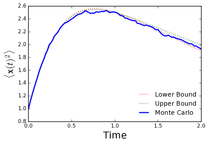
Figure 1: The second moment of the logistic model, (6), using parameters $a_{1}=3$, $b_{1}=1$, $a_{2}=1$, $b_{2}=0$ and initial condition $\boldsymbol{x}(0)=1$. By maximizing and minimizing the bounds on $\langle\boldsymbol{x}(T)^{2}\rangle$ using the SDP from Theorem 1, we get upper and lower bounds on the true value. The result of $5000$ runs of the model are also shown. While we only penalized the final value of $\langle\boldsymbol{x}(T)^{2}\rangle$, the upper and lower bound trajectories have similar values over most of the time horizon. Furthermore, these trajectories both give good approximations to the average trajectory found by Monte Carlo simulations.

Recall the stochastic logistic model from (6). We used Theorem 1 to compute upper and lower bounds on the second moment at the final time, $\langle\boldsymbol{x}(T)^{2}\rangle$. See Fig. 1. Surprisingly, the bounds give a good approximation to $\langle\boldsymbol{x}(t)^{2}\rangle$ for all $t\in[0,T]$, despite only optimizing the bound at the final time, $T$.

Example 12 (Randomly Sampled Feedback – Continued)

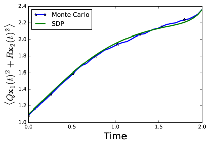
Figure 2: This shows the cost $\langle Q\boldsymbol{x}_{1}(t)^{2}+R\boldsymbol{x}_{2}(t)^{2}\rangle$ averaged over $5000$ runs of the randomly sampled system defined by (13) with $Q=1$ and $R=0.1$. With no feedback, the second moment of $\boldsymbol{x}_{1}(t)$ would increase linearly from $1$ to $3$, and so we would see the final value of the cost to be at least $3$. Note that the SDP cost and the Monte Carlo cost are very close. This is to be expected because the moments are closed in this example.

Recall the sampled-data system from (13) and (14). For $Q=1$ and $R=0.1$, the lower bound from (40) is $3.67$. A linear controller was constructed using the method from Subsection IV-C. This problem has closed moments at second order, and thus we would expect our method to find the exact solution. Fig. 2 shows the cost computed from the SDP as well as the cost found by simulating the computed controller $5000$ times. As expected, the trajectories are very close.

Example 13 (Jump Rate Control – Continued)

Recall the jump rate control problem from Examples 5 and 8. Fig. 3 shows how the control strategy and performance vary as the size of the auxiliary control problem increases. As the order of the auxiliary problem increases, the computed policy begins to resemble an approximate event-triggered policy (19) as predicted from the HJB equation, (18). Furthermore, as the degree of the controller increases, the computed costs appears to approach the steady-state cost predicted from the SDP.

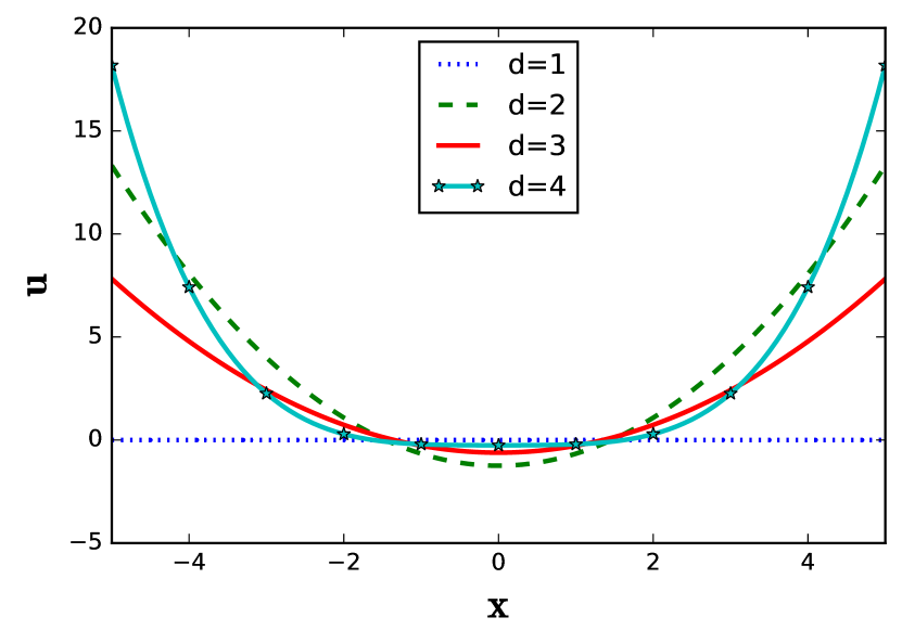
(a) Jump Rate Strategies

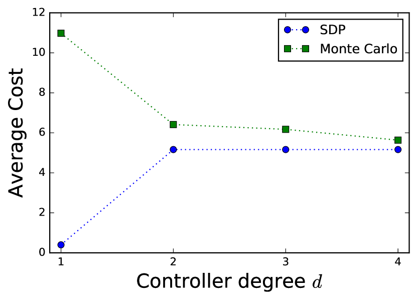
(b) Average Cost

Figure 3: Fig 3 shows the control policies computed as in Subsection IV-C for various orders. Here $Q=1$, $R=10$ and the upper bound on the jump rate $\Omega=10$. Recall from Example 5 that the true optimal controller is an approximate event-trigger control strategy. Specifically, the true optimal policy maintains a zero jump rate for $\boldsymbol{x}(t)$ in some region, and then transitions to a maximum jump rate of $\boldsymbol{u}(t)=\Omega=100$ when $\boldsymbol{x}(t)$ crosses the boundary. As the degree of the controller increases, the strategy becomes flatter near $\boldsymbol{x}(t)=0$ and then increases rapidly for $|\boldsymbol{x}(t)|>5$. As can be seen, the least squares method does not enforce the constraint that $0\leq\boldsymbol{u}(t)\leq\Omega=10$. To get a feasible controller, the value is simply clipped to stay in the correct range. Fig 3 shows the lower bound from the SDP, and compares it with the upper bound given by the feasible controller strategies. As can be seen, the lower bound stops increasing by degree $2$. However, the control strategy from Fig 3 continues to change. The average values from control lead to increasingly tight bounds. The average costs were averaged over $5000$ runs of length $5s$, at a sampling rate of $100Hz$.

Example 14 (Fishery Management – Continued)

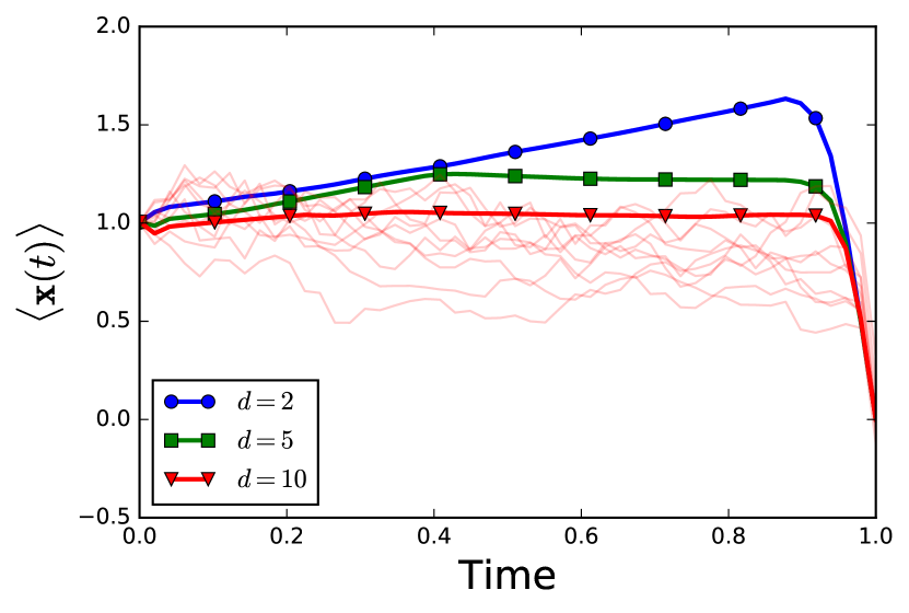
(a) Harvesting Population

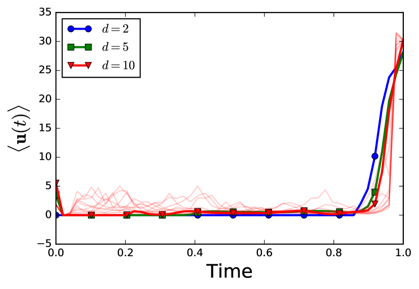
(b) Harvesting Strategy

Figure 4: Figs 4 and 4 the solutions to the optimal harvesting problem. As the order of the controller increases, the following strategy emerges. The controller appears to hold the population at near $\boldsymbol{x}(t)=1$ for most of the time. Then, at the end of the horizon, the population is harvested to extinction.

In this example, the smallest upper bound on the total harvest was computed to be $2.12$, while the lower bound found be simulating the corresponding controller $1000$ times was $1.62$. Thus, the true optimal harvest will likely be in the interval $[1.62,2.12]$. An exact lower bound is not known, since the lower bound was estimated by random sampling. In this example, non-negativity of the state and input were enforced using the vector inequality constraint defined in Lemma 4.

An interesting control strategy appears to emerge, whereby the population is held constant for most of the interval and then fished to extinction at the end of the horizon.

V Conclusion

This paper presented a method based on semidefinite programming for computing bounds on stochastic process moments and stochastic optimal control problems in a unified manner. The method is flexible, in that it can be applied to stochastic differential equations, jump processes and mixtures of the two. Furthermore, systems with and without control inputs can be handled in the same way. The key insight behind the method is the interpretation of the dynamics of the moments as a linear control problem. The auxiliary state consists of a collection of moments of the original state, while the auxiliary input consists of higher order moments required for the auxiliary state, as well as any terms involving inputs to the original system. Then all of the desired bounds can be computed in terms of optimal control problems on this auxiliary system.

Future work will focus on algorithmic improvements and theoretical extensions. A simple algorithmic extension would be to use more general polynomials in the state and input vectors, as opposed to simple monomials. In particular, this would enable the user to choose basis polynomials that offer better numerical stability than the monomials. Methods for automatically constructing the state vectors and constraint matrices are also desirable. In this paper, all of the SDPs were solved using CVXPY [35] in conjunction with off-the-shelf SDP solvers [36, 37]. However, the SDP from (40) has the specialized structure of a linear optimal control problem with LMI constraints. A specialized solver could potentially exploit this structure and enable better scaling. Theoretically, a proof of convergence of the bounds is desirable. For uncontrolled problems, we conjecture that as long as the moments are all finite, the upper and lower bounds converge to the true value. Similarly, for stochastic control problems, we conjecture that the lower bound converges to the true optimal value. Furthermore, the general methodology could potentially be extended to other classes of functions beyond polynomials. In particular, mixtures of polynomials and trigonometric functions seem to be tractable. More generally, it is likely that the method will extend to arbitrary basis function sets that are closed under addition, multiplication, and differentiation.

References

- [1] B. Øksendal, Stochastic differential equations. Springer, 2003.
- [2] B. Øksendal and A. Sulem, Applied Stochastic Control of Jump Diffusions, 3rd ed. Springer, 2009.
- [3] A. G. Malliaris, Stochastic methods in economics and finance. North-Holland, 1982, vol. 17.
- [4] F. B. Hanson, Applied stochastic processes and control for Jump-diffusions: modeling, analysis, and computation. Siam, 2007, vol. 13.
- [5] E. Allen, Modeling with Itô stochastic differential equations. Springer Science & Business Media, 2007, vol. 22.
- [6] E. Theodorou, J. Buchli, and S. Schaal, “A generalized path integral control approach to reinforcement learning,” J. Mach. Learn. Res., vol. 11, pp. 3137–3181, Dec. 2010. [Online]. Available: http://dl.acm.org/citation.cfm?id=1756006.1953033
- [7] G. O. Roberts and R. L. Tweedie, “Exponential convergence of langevin distributions and their discrete approximations,” Bernoulli, pp. 341–363, 1996.
- [8] M. Girolami and B. Calderhead, “Riemann manifold langevin and hamiltonian monte carlo methods,” Journal of the Royal Statistical Society: Series B (Statistical Methodology), vol. 73, no. 2, pp. 123–214, 2011.
- [9] H. Kushner and G. G. Yin, Stochastic approximation and recursive algorithms and applications. Springer Science & Business Media, 2003, vol. 35.
- [10] I. Nåsell, “An extension of the moment closure method,” Theoretical population biology, vol. 64, no. 2, pp. 233–239, 2003.
- [11] A. Singh and J. P. Hespanha, “A derivative matching approach to moment closure for the stochastic logistic model,” Bulletin of mathematical biology, vol. 69, no. 6, pp. 1909–1925, 2007.
- [12] C. Kuehn, Moment Closure–A Brief Review, ser. Understanding Complex Systems, E. Schöll, S. H. Klapp, and P. Hövel, Eds. Springer, 2016.
- [13] L. H. Alvarez and L. A. Shepp, “Optimal harvesting of stochastically fluctuating populations,” Journal of Mathematical Biology, vol. 37, no. 2, pp. 155–177, 1998.
- [14] E. Lungu and B. Øksendal, “Optimal harvesting from a population in a stochastic crowded environment,” Mathematical Biosciences, vol. 145, no. 1, pp. 47 – 75, 1997. [Online]. Available: http://www.sciencedirect.com/science/article/pii/S0025556497000291
- [15] L. Socha, Linearization Methods for Stochastic Dynamic Systems, ser. Lecture Notes in Physics 730. Springer-Verlag, Berlin Heidelberg, 2008.
- [16] A. Singh and J. P. Hespanha, “Lognormal moment closures for biochemical reactions,” in Proceedings of the 45th Conference on Decision and Control, 2006, pp. 2063–2068.
- [17] ——, “Approximate moment dynamics for chemically reacting systems,” IEEE Transactions on Automatic Control, vol. 56, no. 2, pp. 414–418, 2011.
- [18] M. Soltani, C. A. Vargas-Garcia, and A. Singh, “Conditional moment closure schemes for studying stochastic dynamics of genetic circuits,” Biomedical Circuits and Systems, IEEE Transactions on, vol. 9, no. 4, pp. 518–526, 2015.
- [19] A. Lamperski, K. R. Ghusinga, and A. Singh, “Stochastic optimal control using semidefinite programming for moment dynamics,” in Decision and Control (CDC), 2016 IEEE 55th Conference on. IEEE, 2016, pp. 1990–1995.
- [20] J. Kuntz, M. Ottobre, G.-B. Stan, and M. Barahona, “Bounding stationary averages of polynomial diffusions via semidefinite programming,” SIAM Journal on Scientific Computing, vol. 38, no. 6, pp. A3891–A3920, 2016.
- [21] D. P. Bertsekas, Dynamic programming and optimal control. Athena Scientific Belmont, MA, 1995, vol. 1, no. 2.
- [22] W. H. Fleming and H. M. Soner, Controlled Markov Processes and Viscosity Solutions, 2nd ed. Springer, 2006.
- [23] D. P. Bertsekas, Dynamic Programming and Optimal Control: Approximate Dynamic Programming. Athena Scientific, 2012, vol. 2.
- [24] J. B. Lasserre, D. Henrion, C. Prieur, and E. Trélat, “Nonlinear optimal control via occupation measures and LMI-relaxations,” SIAM Journal of COntrol and Optimization, vol. 47, no. 4, pp. 1643 – 1666, 2008.
- [25] A. G. Bhatt and V. S. Borkar, “Occupation measures for controlled markov processes: Characterization and optimality,” The Annals of Probability, pp. 1531–1562, 1996.
- [26] R. Vinter, “Convex duality and nonlinear optimal control,” SIAM journal on control and optimization, vol. 31, no. 2, pp. 518–538, 1993.
- [27] J. B. Lasserre, “Global optimization with polynomials and the problem of moments,” SIAM Journal on Optimization, vol. 11, no. 3, pp. 796–817, 2001.
- [28] L. Rogers, “Pathwise stochastic optimal control,” SIAM Journal on Control and Optimization, vol. 46, no. 3, pp. 1116–1132, 2007.
- [29] D. B. Brown and J. E. Smith, “Information relaxations, duality, and convex stochastic dynamic programs,” Operations Research, vol. 62, no. 6, pp. 1394–1415, 2014.
- [30] G. Jumarie, “A practical variational approach to stochastic optimal control via state moment equations,” Journal of the Franklin Institute, vol. 332, no. 6, pp. 761–772, 1995.
- [31] ——, “Improvement of stochastic neighbouring-optimal control using nonlinear gaussian white noise terms in the taylor expansions,” Journal of the Franklin Institute, vol. 333, no. 5, pp. 773–787, 1996.
- [32] W. Heemels, K. H. Johansson, and P. Tabuada, “An introduction to event-triggered and self-triggered control,” in Decision and Control (CDC), 2012 IEEE 51st Annual Conference on. IEEE, 2012, pp. 3270–3285.
- [33] P. Tabuada, “Event-triggered real-time scheduling of stabilizing control tasks,” IEEE Transactions on Automatic Control, vol. 52, no. 9, pp. 1680–1685, 2007.
- [34] A. V. Rao, “A survey of numerical methods for optimal control,” Advances in the Astronautical Sciences, vol. 135, no. 1, pp. 497–528, 2009.
- [35] S. Diamond and S. Boyd, “CVXPY: A Python-embedded modeling language for convex optimization,” 2016, to appear in Journal of Machine Learning Research. [Online]. Available: http://stanford.edu/~boyd/papers/pdf/cvxpy˙paper.pdf
- [36] B. O’Donoghue, E. Chu, N. Parikh, and S. Boyd, “Conic optimization via operator splitting and homogeneous self-dual embedding,” 2016, to appear in Journal of Optimization Theory and Applications.
- [37] J. Dahl and L. Vandenberghe, “CVXOPT: A python package for convex optimization,” 2008. [Online]. Available: http://www.abel.ee.ucla.edu/cvxopt