KCL-PH-TH/2017-05, CERN-TH/2017-010

KIAS-P17008, UT-17-03

ACT-01-17; MI-TH-1738

UMN-TH-3618/17, FTPI-MINN-17/02

No-Scale SU(5) Super-GUTs

John Ellis^1,2, Jason L. Evans³, Natsumi Nagata⁴,

Dimitri V. Nanopoulos^5,6,7 and Keith A. Olive^8
1Theoretical Physics and Cosmology Group, Department of Physics,
King’s College London, Strand, London WC2R 2LS, UK
²Theoretical Physics Department, CERN, CH-1211 Geneva 23, Switzerland
³School of Physics, KIAS, Seoul 130-722, Korea
⁴Department of Physics, University of Tokyo, Bunkyo-ku, Tokyo 113–0033, Japan
⁵George P. and Cynthia W. Mitchell Institute for Fundamental Physics and Astronomy, Texas A&M University, College Station, TX 77843, USA
⁶Astroparticle Physics Group, Houston Advanced Research Center (HARC),
Mitchell Campus, Woodlands, TX 77381, USA
⁷Academy of Athens, Division of Natural Sciences, Athens 10679, Greece
⁸William I. Fine Theoretical Physics Institute, School of Physics and Astronomy,
University of Minnesota, Minneapolis, MN 55455, USA

Abstract

We reconsider the minimal SU(5) Grand Unified Theory (GUT) in the context of no-scale supergravity, assuming that the soft supersymmetry-breaking parameters satisfy universality conditions at some input scale $M_{\rm in}$ above the GUT scale $M_{GUT}$. When setting up such a no-scale super-GUT model, special attention must be paid to avoiding the Scylla of rapid proton decay and the Charybdis of an excessive density of cold dark matter, while also having an acceptable mass for the Higgs boson. We do not find consistent solutions if none of the matter and Higgs fields are assigned to twisted chiral supermultiplets, even in the presence of Giudice-Masiero terms. However, consistent solutions may be found if at least one fiveplet of GUT Higgs fields is assigned to a twisted chiral supermultiplet, with a suitable choice of modular weights. Spin-independent dark matter scattering may be detectable in some of these consistent solutions.

February 2017

1 Introduction

Globally supersymmetric grand unification has long been an attractive framework for unifying the non-gravitational interactions, with the minimal option using the gauge group SU(5) [1, 2]. When incorporating gravity, one must embed such a supersymmetric Grand Unified Theory (GUT) within some supergravity theory, and an attractive option is no-scale supergravity [3]. This has the advantages that it leads to an effective potential without holes of depth ${\cal O}(1)$ in natural units, and emerges in generic string compactifications [4]. No-scale supergravity also allows naturally for the possibility of Planck-compatible cosmological inflation [5]. In general, a no-scale Kähler potential contains several moduli $T_{i}$, but here we consider scenarios in which the relevant dynamics is dominated by a single volume modulus field $T$.

The construction of no-scale supergravity GUTs encounters significant hurdles, such as fixing the compactification moduli. Moreover, pure no-scale boundary conditions require that all the quadratic, bilinear and trilinear scalar couplings $m_{0},B_{0}$ and $A_{0}$ vanish, leading to phenomenology that is in contradiction with experimental constraints. However, this issue may be avoided in models with (untwisted or twisted) matter fields with non-vanishing modular weights as we show below.

The simplest possibility for soft supersymmetry breaking is to postulate universal values of $m_{0},B_{0}$ and $A_{0}$, as in the constrained minimal supersymmetric Standard Model (CMSSM) [6, 7, 8, 9]. With the inclusion of a universal gaugino mass, $m_{1/2}$, the CMSSM is a four-parameter theory. Minimal supergravity places an additional boundary condition, relating $B_{0}$ and $A_{0}$ ($B_{0}=A_{0}-m_{0}$) making it a three-parameter theory [10, 11]. No-scale supergravity, however is effectively a one-parameter theory since we require $m_{0}=A_{0}=B_{0}=0$. Another one-parameter theory in this context is pure gravity mediation [12, 13, 14], in which the gaugino masses, $A$ and $B$ terms are determined by anomaly mediation [16] leaving only the gravitino mass, $m_{3/2}=m_{0}$ as a free parameter.

These boundary conditions may be too restrictive if they are imposed at the GUT scale, $M_{GUT}$, defined as the renormalization scale where the two electroweak gauge couplings are unified. There is, however, no intrinsic reason that the boundary conditions for supersymmetry breaking coincide with gauge coupling unification. Separating these two scales opens the door for so-called sub-GUT models [17, 8, 9] where the input universality scale differs from the GUT scale with $M_{in}<M_{GUT}$ or the possibility that the boundary conditions are imposed at some higher input scale $M_{\rm in}>M_{GUT}$, a scenario we term super-GUT [18, 19].

However, the regions of parameter space with acceptable relic density and Higgs mass typically require quite special values of the GUT superpotential couplings and rather large values of $\tan\beta$ [20], and hence a proton lifetime that is unacceptably short. In order to accommodate smaller values of $\tan\beta$ and hence an acceptably long proton lifetime, we consider non-zero Giudice-Masiero (GM) terms [15] in the Kähler potential. In this way we are able to avoid the Scylla of rapid proton decay and the Charybdis of an excessive density of cold dark matter, while also having an acceptable value of the Higgs mass. Furthermore, when no-scale boundary conditions are applied at the GUT scale, the lightest sparticle in the spectrum is typically a stau (or the stau is tachyonic). Applying the boundary conditions above the GUT scale as in a super-GUT model can alleviate this problem [21].

The outline of this paper is as follows. In Section 2, we review our theoretical framework, with our set-up of the minimal supersymmetric SU(5) model described in Subsection 2.1, our no-scale supergravity framework described in Subsection 2.2 and the vacuum conditions and the relevant renormalization-group equations (RGEs) set out in Subsection 2.3. We describe our key results in Section 3. We explore in Section 3.1 scenarios in which none of the matter and Higgs supermultiplets are twisted, and find no way to steer between Scylla and Charybdis with an acceptable Higgs mass in this case. However, as we show in Section 3.2, this is quite possible if one or the other (or both) of the GUT fiveplet Higgs supermultiplets is twisted. Spin-independent dark matter scattering may be observable in some of the cases studied. Finally, Section 4 discusses our results.

2 Super-GUT CMSSM Models

2.1 Minimal Supersymmetric SU(5)

The minimal supersymmetric SU(5) GUT [2], was recently reviewed in [19] and we recall here the aspects most needed for our discussion. The minimal renormalizable superpotential for this model is given by

$$W_{5} =\mu_{\Sigma}{\rm Tr}\Sigma^{2}+\frac{1}{6}\lambda^{\prime}{\rm Tr}\Sigma^{3}+\mu_{H}\overline{H}H+\lambda\overline{H}\Sigma H$$

$$+\left(h_{\bf 10}\right)_{ij}\epsilon_{\alpha\beta\gamma\delta\zeta}\Psi_{i}^{\alpha\beta}\Psi^{\gamma\delta}_{j}H^{\zeta}+\left(h_{\overline{\bf 5}}\right)_{ij}\Psi_{i}^{\alpha\beta}\Phi_{j\alpha}\overline{H}_{\beta}~{},$$ (1)

where Greek sub- and superscripts denote SU(5) indices, and $\epsilon$ is the totally antisymmetric tensor with $\epsilon_{12345}=1$. In Eq. (1), the adjoint multiplet $\Sigma\equiv\sqrt{2}\Sigma^{A}T^{A}$, where the $T^{A}$ ($A=1,\dots,24$) are the generators of SU(5) normalized so that ${\rm Tr}(T^{A}T^{B})=\delta_{AB}/2$, is responsible for breaking SU(5) to the Standard Model (SM). The scalar components of $\Sigma$ are assumed to have vevs of the form

$$\langle\Sigma\rangle=V\cdot{\rm diag}\left(2,2,2,-3,-3\right)~{},$$ (2)

where $V\equiv 4\mu_{\Sigma}/\lambda^{\prime}$, causing the GUT gauge bosons $X$ to acquire masses $M_{X}=5g_{5}V$, where $g_{5}$ is the SU(5) gauge coupling.

The multiplets $H$ and $\overline{H}$ in Eq. (1) are ${\bf 5}$ and $\overline{\bf 5}$ representations of SU(5), respectively, and contain the MSSM Higgs fields. In order to realize doublet-triplet mass splitting in the $H$ and $\overline{H}$ multiplets, we impose the fine-tuning condition $\mu_{H}-3\lambda V\ll V$. In this case, the color-triplet Higgs states have masses $M_{H_{C}}=5\lambda V$, the masses of the color and weak adjoint components of $\Sigma$ are $M_{\Sigma}=5\lambda^{\prime}V/2$, and the singlet component of $\Sigma$ acquires a mass $M_{\Sigma_{24}}=\lambda^{\prime}V/2$.

The multiplets ${\Phi}_{i}$ in Eq. (1) are $\bf{\overline{5}}$ representations containing the left-handed SM matter fields $\overline{D}_{i}$ and ${L}_{i}$, and the ${\Psi}_{i}$ are $\bf{10}$ representations of SU(5) containing the left-handed ${Q}_{i}$, $\overline{U}_{i}$, and $\overline{E}_{i}$, where the index $i=1,2,3$ denotes the generations.

The soft supersymmetry-breaking terms in the minimal supersymmetric SU(5) GUT are

$${\cal L}_{\rm soft}= -\left(m_{\bf 10}^{2}\right)_{ij}\widetilde{\psi}_{i}^{*}\widetilde{\psi}_{j}-\left(m_{\overline{\bf 5}}^{2}\right)_{ij}\widetilde{\phi}^{*}_{i}\widetilde{\phi}_{j}-m_{H}^{2}|H|^{2}-m_{\overline{H}}^{2}|\overline{H}|^{2}-m_{\Sigma}^{2}{\rm Tr}\left(\Sigma^{\dagger}\Sigma\right)$$

$$-\biggl{[}\frac{1}{2}M_{5}\widetilde{\lambda}^{A}\widetilde{\lambda}^{A}+A_{\bf 10}\left(h_{\bf 10}\right)_{ij}\epsilon_{\alpha\beta\gamma\delta\zeta}\widetilde{\psi}_{i}^{\alpha\beta}\widetilde{\psi}^{\gamma\delta}_{j}H^{\zeta}+A_{\overline{\bf 5}}\left(h_{\overline{\bf 5}}\right)_{ij}\widetilde{\psi}_{i}^{\alpha\beta}\widetilde{\phi}_{j\alpha}\overline{H}_{\beta}$$

$$+B_{\Sigma}\mu_{\Sigma}{\rm Tr}\Sigma^{2}+\frac{1}{6}A_{\lambda^{\prime}}\lambda^{\prime}{\rm Tr}\Sigma^{3}+B_{H}\mu_{H}\overline{H}H+A_{\lambda}\lambda\overline{H}\Sigma H+{\rm h.c.}\biggr{]}~{},$$ (3)

where $\widetilde{\psi}_{i}$ and $\widetilde{\phi}_{i}$ are the scalar components of $\Psi_{i}$ and $\Phi_{i}$, respectively, the $\widetilde{\lambda}^{A}$ are the SU(5) gauginos. We use the same symbols for the scalar components of the Higgs fields as for the corresponding superfields.

2.2 No-Scale Framework

We refer to [22] for a derivation of the soft terms arising in no-scale supergravity . Our starting-point is a no-scale Kähler potential

$$K\;=\;-3\ln\left(T+{\bar{T}}-\frac{1}{3}\sum_{i}|\phi_{i}|^{2}\right)+\sum_{a}\frac{|\varphi_{a}|^{2}}{(T+{\bar{T}})^{n_{a}}}\,,$$ (4)

which includes a volume modulus field, $T$, and both untwisted and twisted matter fields, $\phi_{i}$ and $\varphi_{a}$ respectively, the latter with modular weights $n_{a}$. We consider a generic superpotential of the form

$$W =(T+c)^{\beta}W_{2}(\phi_{i})+(T+c)^{\alpha}W_{3}(\phi_{i})$$ (5)

$$\qquad+(T+c)^{\sigma}W_{2}(\varphi_{a})+(T+c)^{\rho}W_{3}(\varphi_{a})+\mu_{\Lambda}\,,$$

where $c$ is an arbitrary constant, and $W_{2,3}$ denote bilinear and trilinear terms with modular weights that are in general non-zero. When $\langle\phi,\varphi\rangle=0$, the effective potential for $T$ is completely flat at the tree level, so it has an undetermined vev, and the gravitino mass

$$m_{3/2}=\frac{\mu_{\Lambda}}{(T+\bar{T})^{3/2}}$$ (6)

varies with the value of this volume modulus. We assume here that some Planck scale dynamics fixes $T=\bar{T}=c$, and take $c=1/2$ in the following.

In a standard no-scale supergravity model with no twisted fields and with weights $\alpha=\beta=0$, we would obtain $m_{0}=A_{0}=B_{0}=0$. However, in the scenario (5) soft terms are induced, as were calculated in [22], which are sector-dependent:

$$\phi_{i}: \quad m_{0}=0\ ,\quad B_{0}=-\beta m_{3/2}\ ,\quad A_{0}=-\alpha m_{3/2}\,,$$ (7)

$$\varphi_{a}: \quad m_{0}=m_{3/2}\ ,\quad B_{0}=2m_{3/2}\left(1-\frac{\sigma}{2}\right)\ ,\qquad A_{0}=3m_{3/2}\left(1-\frac{\rho}{3}\right)\,,$$ (8)

where we have assumed for simplicity that $n_{a}=0$. We also postulate in what follows generalized Giudice-Masiero terms [15]

$$\Delta K=\left(c_{H}(T+c)^{\gamma_{H}}H\bar{H}+c_{\Sigma}(T+c)^{\gamma_{\Sigma}}\Sigma^{2}+{\rm h.c.}\right).$$ (9)

If $H$, $\bar{H}$, and $\Sigma$ are untwisted, these induce corrections to the $\mu$ and $B$ terms:

$$\Delta\mu_{H}=c_{H}m_{3/2}\ ,~{}~{}\Delta\mu_{\Sigma}=c_{\Sigma}m_{3/2}\ ,~{}~{}\Delta B_{H}\mu_{H}=-\gamma_{H}c_{H}m_{3/2}^{2}\ ,~{}~{}\Delta B_{\Sigma}\mu_{\Sigma}=-\gamma_{\Sigma}c_{\Sigma}m_{3/2}^{2}.$$ (10)

If the fields are twisted, the shift in the $\mu$-terms is the same, but the shift in $B\mu$ is modified by $-\gamma_{H,\Sigma}c_{H,\Sigma}\to(2-\gamma_{H,\Sigma})c_{H,\Sigma}$ [22]. Although the corrections to the $B$ terms are quite small, they are crucial for matching the GUT scale $B$ terms onto the MSSM $B$ term at the GUT scale, as we see below.

In the super-GUT version of the CMSSM model we impose the following universality conditions for the soft mass parameters at a soft supersymmetry-breaking mass input scale $M_{in}>M_{\rm GUT}$:

$$\left(m_{\bf 10}^{2}\right)_{ij}=\left(m_{\overline{\bf 5}}^{2}\right)_{ij} \equiv m_{0}^{2}\,\delta_{ij}~{},$$

$$m_{H}=m_{\overline{H}}=m_{\Sigma} \equiv m_{0}~{},$$

$$A_{\bf 10}=A_{\overline{\bf 5}}=A_{\lambda}=A_{\lambda^{\prime}} \equiv A_{0}~{},$$

$$B_{H}=B_{\Sigma} \equiv B_{0}~{},$$

$$M_{5} \equiv m_{1/2}~{},$$ (11)

with the input soft terms $m_{0},A_{0}$ and $B_{0}$ specified above. In the above expressions, and in expressions throughout the text, the $\Delta B$ contribution is neglected since it is so small. However, this contribution to the $B$-terms is included in all calculations in order to satisfy the $B$-term matching condition.

2.3 Vacuum Conditions and Renormalization-Group Equations

Since the $B$-term boundary conditions are specified at $M_{in}$, we cannot use the Higgs minimization equations to determine $B$ and the MSSM $\mu$ term as is commonly done in the MSSM. Instead, as in mSUGRA models, these conditions can be used to determine $\mu$ and $\tan\beta$ [11] as was done in the no-scale super-GUT models considered in [20]. In [20], standard no-scale boundary conditions were used to identify regions of parameter space with acceptable relic density and Higgs mass. Typically, rather large values of $\tan\beta$ were found and, in addition, it was necessary to choose somewhat small values of the coupling $\lambda={\cal O}(0.01)$ with much larger values of $\lambda^{\prime}={\cal O}(1)$. All of these choices tend to decrease the proton lifetime to unacceptably small values [19]. In order to reconcile the proton lifetime with the relic density and Higgs mass, we need to consider lower values of $\tan\beta$ [24, 9, 19], which can be accomplished when the GM terms (9) are included [15, 25, 13, 14].

The soft supersymmetry breaking parameters are evolved down from $M_{in}$ to $M_{GUT}$ using the renormalization-group equations (RGEs) of the minimal supersymmetric SU(5) GUT, which can be found in [26, 27, 18, 20, 28], with appropriate changes of notation. During the evolution, the GUT couplings in Eq. (1) affect the running of the soft supersymmetry-breaking parameters, which results in non-universality in the soft parameters at $M_{GUT}$. In particular, the GUT coupling $\lambda$ contributes to the running of the Yukawa couplings, the corresponding $A$-terms, and the Higgs soft masses. On the other hand, $\lambda^{\prime}$ affects directly only the running of $\lambda$, $m_{\Sigma}$, and $A_{\lambda}$ (besides $\lambda^{\prime}$ and $A_{\lambda^{\prime}}$), and thus can affect the MSSM soft mass parameters only at higher-loop level. Both $\lambda$ and $\lambda^{\prime}$ contribute to the RGEs of the soft masses of matter multiplets only at higher-loop level, suppressing their effects on these parameters.

At the unification scale $M_{GUT}$ (defined as the renormalization scale where the two electroweak gauge couplings are equal), the SU(5) GUT parameters are matched onto the MSSM parameters. The matching conditions for the Standard Model gauge and Yukawa couplings were discussed in detail in [19]. The use of threshold corrections at the GUT scale [29, 30, 31] allow us to determine the SU(5) gauge coupling, $g_{5}$, and the SU(5) Higgs adjoint vev, $V$, which in turn allows us to fix the gauge and Higgs boson masses as

$$M_{H_{C}} =5\lambda V~{},$$ (12)

$$M_{\Sigma} =\frac{5}{2}\lambda^{\prime}V~{},$$ (13)

$$M_{X} =5g_{5}V~{},$$ (14)

which are inputs in the calculation of the proton lifetime.

As explained in [19], in order to allow both $\lambda$ and $\lambda^{\prime}$ to remain as free parameters, we must include a Planck-suppressed operator such as

$$W_{\rm eff}^{\Delta g}=\frac{c_{5}}{M_{P}}{\rm Tr}\left[\Sigma{\cal W}{\cal W}\right]~{},$$ (15)

where ${\cal W}\equiv T^{A}{\cal W}^{A}$ denotes the superfields corresponding to the field strengths of the SU(5) gauge vector bosons. Such operators may make contributions comparable to other threshold corrections when $\Sigma$ develops a vev [32, 33, 34]. We have checked that the coefficient $c_{5}$ takes reasonable values, i.e., $|c_{5}|<{\cal O}(1)$.

The matching conditions for the soft supersymmetry-breaking terms were also discussed in detail in [19]. The matching conditions for the gaugino masses [34, 35] are given by

$$M_{1} =\frac{g_{1}^{2}}{g_{5}^{2}}M_{5}-\frac{g_{1}^{2}}{16\pi^{2}}\left[10M_{5}+10(A_{\lambda^{\prime}}-B_{\Sigma})+\frac{2}{5}B_{H}\right]+\frac{4c_{5}g_{1}^{2}V(A_{\lambda^{\prime}}-B_{\Sigma})}{M_{P}}~{},$$ (16)

$$M_{2} =\frac{g_{2}^{2}}{g_{5}^{2}}M_{5}-\frac{g_{2}^{2}}{16\pi^{2}}\left[6M_{5}+6A_{\lambda^{\prime}}-4B_{\Sigma}\right]+\frac{12c_{5}g_{2}^{2}V(A_{\lambda^{\prime}}-B_{\Sigma})}{M_{P}}~{},$$ (17)

$$M_{3} =\frac{g_{3}^{2}}{g_{5}^{2}}M_{5}-\frac{g_{3}^{2}}{16\pi^{2}}\left[4M_{5}+4A_{\lambda^{\prime}}-B_{\Sigma}+B_{H}\right]-\frac{8c_{5}g_{3}^{2}V(A_{\lambda^{\prime}}-B_{\Sigma})}{M_{P}}~{}.$$ (18)

We again find that the contribution of the dimension-five operator in Eq. (15) can be comparable to that of the one-loop threshold corrections. MSSM soft masses and the $A$-terms of the third generation sfermions, are given by

$$m^{2}_{Q}=m_{U}^{2}=m^{2}_{E}=m^{2}_{{\bf 10}}~{}, ~{}~{}~{}~{}~{}~{}m_{D}^{2}=m_{L}^{2}=m_{\overline{\bf 5}}^{2}~{},$$

$$m_{2}\equiv m_{H_{u}}^{2}=m_{H}^{2}~{}, ~{}~{}~{}~{}~{}~{}m_{1}\equiv m_{H_{d}}^{2}=m_{\overline{H}}^{2}~{},$$

$$A_{t}=A_{\bf 10}~{}, ~{}~{}~{}~{}~{}~{}A_{b}=A_{\tau}=A_{\overline{\bf 5}}~{}.$$ (19)

The MSSM $\mu$ and $B$ terms are [36]

$$\mu =\mu_{H}-3\lambda V\left[1+\frac{A_{\lambda^{\prime}}-B_{\Sigma}}{2\mu_{\Sigma}}\right]~{},$$ (20)

$$B =B_{H}+\frac{3\lambda V\Delta}{\mu}+\frac{6\lambda}{\lambda^{\prime}\mu}\left[(A_{\lambda^{\prime}}-B_{\Sigma})(2B_{\Sigma}-A_{\lambda^{\prime}}+\Delta)-m_{\Sigma}^{2}\right]~{},$$ (21)

with

$$\Delta\equiv A_{\lambda^{\prime}}-B_{\Sigma}-A_{\lambda}+B_{H}~{}.$$ (22)

The amount of fine-tuning required to obtain values of $\mu$ and $B$ that are ${\cal O}(M_{\rm SUSY})$ is determined by these last two equations. From Eq. (20), we find that we need to tune $|\mu_{H}-3\lambda V|$ to be ${\cal O}(M_{\rm SUSY})$. From Eq. (21), $V\Delta/\mu$ should be ${\cal O}(M_{\rm SUSY})$, which requires $|\Delta|\leq{\cal O}(M_{\rm SUSY}^{2}/M_{GUT})$. In standard no-scale supergravity, $\Delta=0$ and this is stable against radiative corrections, as shown in Ref. [37]. As discussed in Ref. [19], in order for Eq. (21) to have a real solution for $B_{\Sigma}$, the condition $A_{\lambda^{\prime}}^{2}\gtrsim 8m_{\Sigma}^{2}$ should be satisfied for $\lambda^{\prime}\ll\lambda$. We have checked that this condition is always satisfied over the parameter space we consider in Section 3.

The MSSM $\mu$ and $B$ parameters can be determined by using the electroweak vacuum conditions:

$$\mu^{2} =\frac{m_{1}^{2}-m_{2}^{2}\tan^{2}\beta+\frac{1}{2}m_{Z}^{2}(1-\tan^{2}\beta)+\Delta_{\mu}^{(1)}}{\tan^{2}\beta-1+\Delta_{\mu}^{(2)}},$$ (23)

$$B\mu =-\frac{1}{2}(m_{1}^{2}+m_{2}^{2}+2\mu^{2})\sin 2\beta+\Delta_{B}~{},$$ (24)

where $\Delta_{B}$ and $\Delta_{\mu}^{(1,2)}$ denote loop corrections [38]. These are run up to the GUT scale where the conditions (20) and (21) are applied. However, in standard no-scale supergravity, the right-hand side of (21) is determined by running down the $A$ and $B$-terms set by $A_{0}=B_{0}=0$ (and similarly for $m_{\Sigma}^{2}$). Thus, (21) is not satisfied in general. Nevertheless, it is often possible to find a value of $\tan\beta$ that adjusts $B\mu$ via (24) to have the correct value at the GUT scale. As noted earlier, this often leads to relatively large values of $\tan\beta$ and unacceptable low values for the proton lifetime.

Alternatively, we can introduce a GM term in the Kähler potential as in Eq. (9). For now, we assume that all fields are untwisted with weight $\gamma=-1$. The shift in the $\mu$-terms is ${\cal O}(M_{\rm SUSY})$ and is irrelevant to the matching condition (20). Similarly the shifts in most of the terms in (21) are of order $m_{3/2}^{2}/M_{GUT}$ and are much smaller than ${\cal O}(M_{\rm SUSY})$. However, there is a shift in $\Delta$

$$\delta\Delta=\left(\frac{c_{H}}{\mu_{H}}-\frac{c_{\Sigma}}{\mu_{\Sigma}}\right)m_{3/2}^{2}.$$ (25)

Although this shift is also small, $\Delta$ is multiplied by $V/\mu$ in (21), so that the overall shift in $B$ is ${\cal O}(M_{\rm SUSY})$. Thus the shift in (21) becomes

$$\frac{3\lambda V\Delta}{\mu}\to\left(c_{H}-\frac{12\lambda}{\lambda^{\prime}}c_{\Sigma}\right)\frac{m_{3/2}^{2}}{\mu},$$ (26)

up to ${\cal O}(M_{\rm SUSY}/M_{\rm GUT})$ corrections. This is now of comparable size to other terms in (21), which can be satisfied for any $\tan\beta$. The matching condition (21), therefore determines a linear combination of the two GM terms.

Our no-scale super-GUT model is therefore specified by the following set of input parameters:

$$m_{1/2},\ M_{in},\ \lambda,\ \lambda^{\prime},\ \tan\beta,\ {\rm sign}(\mu)\,,$$ (27)

where the trilinear superpotential Higgs couplings, $\lambda$ and $\lambda^{\prime}$, are specified at $Q=M_{GUT}$.

In the following we assume initially that all fields are untwisted, so that $m_{0}=0$, and assume vanishing modular weights $\alpha=\beta=0$, so that $A_{0}=B_{0}=0$. Later we consider the effects of twisting one or both of the Higgs 5-plets and turning on the trilinear weight $\alpha$ in order to allow non-zero $A_{0}$.

3 Results

3.1 Standard No-scale Supergravity with a GM Term

It is well known that the CMSSM with no-scale boundary conditions is not viable. With $m_{0}=A_{0}=B_{0}=0$, the particle spectrum almost inevitably contains either a stau lightest supersymmetric particle (LSP) or tachyonic stau. However, this problem can be alleviated if the universal boundary conditions are applied above the GUT scale [21]. In this case, the running from $M_{\rm in}$ to $M_{\rm GUT}$ produces non-zero soft terms that may be sufficiently large to produce a reasonable spectrum .

The basic no-scale super-GUT model was studied in detail in [20]. There it was found that, for sufficiently large $M_{\rm in}$, not only could a reasonable mass spectrum be obtained, but also regions of parameter space with the correct relic density and Higgs mass were identified. This region was further explored in [40], with the aim of studying possible departures from minimal flavor violation. There, for example, a particular benchmark point was chosen with $M_{5}=1500$ GeV, $M_{\rm in}=10^{18}$ GeV, $\lambda=-0.1,\lambda^{\prime}=2$, which required $\tan\beta\approx 52$ as no GM term was included. One concern for this benchmark is the proton decay rate that is enhanced by the combination of large $\tan\beta$ and small $\lambda$ (which induced a low value for the Higgs color triplet mass). Indeed, as we show below, the proton lifetime is far too small in this minimal SU(5) construction.

We show in Fig. 1 two examples of $(m_{1/2},\tan\beta)$ planes for fixed $M_{\rm in}=10^{18}$ GeV. In the left panel, we have chosen $\lambda=-0.1$ and $\lambda^{\prime}=2$. In the dark blue shaded strip, the neutralino LSP relic density agrees with the value determined by Planck and other experiments. To its left, in the brown shaded region the stau is either the LSP or tachyonic. The red dot-dashed contours show the value of the Higgs mass as computed using the FeynHiggs code [41] . As one can see, there is a region at large $\tan\beta\in 52$–55 for $m_{1/2}\in 1$–1.5 TeV that corresponds to the preferred region found in [20] . In this region the Higgs mass $\in 122$–124 GeV, which is acceptable given the uncertainty in the mass calculated using FeynHiggs. By including a GM term, we are able to probe lower values of $\tan\beta$ for the same set of input parameters. Unfortunately, the proton lifetime is much too small over the entire left panel, with a value of only $10^{25}$ yrs in the upper left corner. We also show (in green) the contours of the GM term. In this case, since $|\lambda|\lesssim\lambda^{\prime}$, we assume $c_{H}=0$ and show the contours of $c_{\Sigma}(m_{3/2}/m_{1/2})^{2}$ . As one can see, the contour for $c_{\Sigma}=0$ runs through the region of good relic density and Higgs mass found in [20].

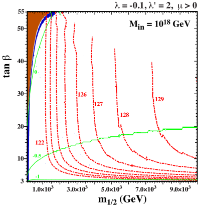
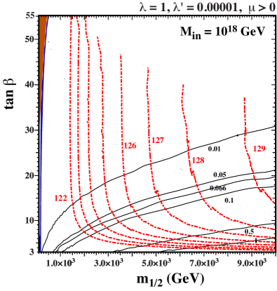
Figure 1: Sample no-scale super-GUT $(m_{1/2},\tan\beta)$ planes for $M_{\rm in}=10^{18}$ GeV. In the left panel $\lambda=-0.1$ and $\lambda^{\prime}=2$, whereas in the right panel $\lambda=1$ and $\lambda^{\prime}=10^{-5}$. The brown shaded region has a stau LSP. The regions compatible with the relic density determined by Planck and other experiments are shaded dark blue, and the red dot-dashed curves are contours of constant Higgs mass as calculated using FeynHiggs, which does not give stable results in the upper right portions of the panels. In the left panel, the green curves are contours of $c_{\Sigma}(m_{3/2}/m_{1/2})^{2}$ and the proton lifetime is too short throughout. In the right panel, the solid black contours show the proton lifetime in units of $10^{35}$ yrs, which is acceptably long below the contour labelled 0.066. However, the relic density is too large throughout this region.

In the right panel of Fig. 1 we show a similar plane but with different choices of $(\lambda,\lambda^{\prime})=(1,10^{-5})$, which are more typical of the values required in [19]. In this case, with $\lambda\gg\lambda^{\prime}$, the value of $c_{\Sigma}(m_{3/2}/m_{1/2})^{2}$ is very near $-0.25$ all across the plane. As long as $c_{H}$ is relatively small, one can see from Eq. (26) that the value of $c_{H}$ has little effect on our estimate of $c_{\Sigma}(m_{3/2}/m_{1/2})^{2}$ which are quoted assuming $c_{H}=0$. The large ratio of $\lambda/\lambda^{\prime}$ is beneficial for increasing the proton lifetime, and contours showing the lifetime are seen as solid black curves in the lower right portion of the panel, labelled in units of $10^{35}$ yrs ; as the current experimental limit is $\tau(p\to K^{+}\overline{\nu})>6.6\times 10^{33}$ yrs [44], the region with acceptable proton stability lies below the contour labelled 0.066. Whilst it is encouraging that some region of parameter space exists with a sufficiently long proton lifetime and acceptable Higgs mass, the relic density is far too large in this region: $\Omega h^{2}\sim\mathcal{O}(100)$. Further exploration in the ($M_{\rm in},\lambda,\lambda^{\prime}$) parameter space does not yield better results. The Higgs mass can be made compatible with either the relic density or the proton lifetime, but not both.

The left panel of Fig. 1 shows that, at fixed $m_{1/2}$, the value of $m_{h}$ decreases rapidly when $\tan\beta\lesssim 10$. On the other hand, the right panel of Fig. 1 shows that the proton lifetime is unacceptably short for $\tan\beta\gtrsim 10$. As we discuss below with several examples, these two problems can be avoided simultaneously when $\tan\beta=7$, for suitable choices of the other super-GUT model parameters $M_{in},\lambda$ and $\lambda^{\prime}$. We do not discuss in the following possible variations in the value of $\tan\beta$, but have checked that values differing from 7 by factors $\gtrsim 2$ are typically excluded by either $m_{h}$ or the proton lifetime.

3.2 Twisted $H$ and $\overline{H}$ Higgs Fields

In this subsection we consider departures from the minimal model discussed above that allow for more successful phenomenology. We start by considering the consequences of a twisted Higgs sector. As discussed above, $\tan\beta$ must be relatively low to obtain sufficiently long proton lifetimes. However, in order to obtain a sufficiently large Higgs mass, $\tan\beta$ should not be too low. Choosing $\tan\beta=7$ with $\lambda^{\prime}=10^{-5}$ optimizes both $m_{h}$ and $\tau_{p}$, so we fix those values for now. In the following, we take $\lambda=0.6$ and 1.

The superpotential (5) does not cover the case where twisted fields couple to untwisted fields. If the Higgs 5-plets are twisted, then $W_{3}$ contains Yukawa couplings between the twisted Higgses and untwisted matter fields. In addition, if $\Sigma$ remains untwisted, then $W_{3}$ also contains a term coupling one untwisted field ($\Sigma$) and the twisted Higgs fields. We define weights for each of the terms in $W_{3}$: $\alpha_{t}$, $\alpha_{b}$, $\alpha_{\lambda}$, and $\alpha_{\lambda}^{\prime}$ corresponding to the top and bottom Yukawa couplings, the coupling of the Higgs adjoint to the 5-plets, and the adjoint trilinear, respectively. Similarly, we define separate weights $\beta_{H}$ and $\beta_{\Sigma}$ for the two bilinears in $W_{2}$. When both $H$ and $\overline{H}$ are twisted, $A$ and $B$ terms are given at the input renormalization scale by

$$A_{t,b}=(1-\alpha_{t,b})m_{3/2}~{},\qquad A_{\lambda}=(2-\alpha_{\lambda})m_{3/2}~{},\qquad A_{\lambda^{\prime}}=-\alpha_{\lambda^{\prime}}m_{3/2}\,,$$ (28)

and

$$B_{H}=(2-\beta_{H})m_{3/2}~{},\qquad B_{\Sigma}=-\beta_{\Sigma}m_{3/2}\,.$$ (29)

The Higgs soft squared masses are given by $m_{3/2}^{2}$ in addition to the usual supersymmetric contribution from $\mu$ (properly shifted by the GM term).

We consider first the case where both Higgs 5-plets are twisted, and therefore receive equal soft supersymmetry breaking masses, $m_{1}=m_{2}=m_{3/2}$. We start by taking all of the modular weights $\alpha=\beta=0$ as before. Now, however, there are non-zero $A$ and $B$ terms at the input scale. We assume $A_{t,b}=m_{3/2}$, $A_{\lambda}=2m_{3/2}$, $A_{\lambda^{\prime}}=0$, $B_{H}=2m_{3/2}$ and $B_{\Sigma}=0$ at the input renormalization scale, $M_{in}$. The ($m_{1/2},m_{1}$) plane for this case with $M_{\rm in}=M_{\rm GUT}$ is shown in the left panel of Fig. 2. This is the limiting case in which the super-GUT scenario reduces to an NUHM1 plane [45, 46, 8, 9] with $m_{0}=0$ and $A_{0}=m_{1}$. Note that the values of $\lambda$ and $\lambda^{\prime}$ are irrelevant when taking $M_{\rm in}=M_{\rm GUT}$ as there is no running above the GUT scale in this case. There is narrow band where the LSP is the lightest neutralino and the electroweak symmetry breaking conditions can be satisfied, through which runs a blue relic density strip. At low values of $m_{1/2}$, the relic density is determined by stau coannihilation [47], and the blue relic density strip lies close to the boundary of the stau LSP region (shaded red). At higher $m_{1/2}$, the strip moves closer to the region with no electroweak symmetry breaking (shaded pink) and becomes a focus-point strip [48]. The Higgs mass (shown by the red dot-dashed contours between the two excluded regions) has acceptable values along much of the relic density strip. On the other hand, the proton lifetime is too short as the entire strip shown lies at or below the contour corresponding to $\tau_{p}=0.001\times 10^{35}$ yrs (which appears as the black curve that enters the allowed region at about 5 TeV at an angle to the relic density strip). The right panel of Fig. 2 shows the corresponding plane with the following choices of modular weights: $\alpha_{t,b}=1$, $\alpha_{\lambda}=2$, $\alpha_{\lambda^{\prime}}=0$, $\beta_{H}=2$ and $\beta_{\Sigma}=0$, which correspond to $A_{0}=B_{0}=0$. This exhibits many features similar to the left panel. In particular, the relic density and proton lifetime constraints are incompatible, motivating our exploration of super-GUT scenarios.

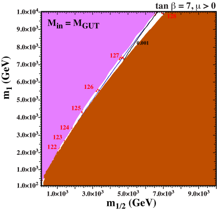
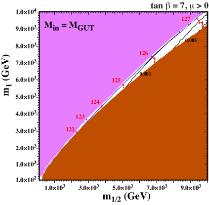
Figure 2: Examples of $(m_{1/2},m_{1})$ planes for $M_{\rm in}=M_{\rm GUT}$ and $\tan\beta=7$ when both Higgs 5-plets are twisted. In the left panel, all the modular weights $\alpha_{i}=\beta_{i}=0$, corresponding to $A_{t,b}=m_{1}$, $A_{\lambda}=2m_{3/2}$, $A_{\lambda^{\prime}}=0$, $B_{H}=2m_{1}$, and $B_{\Sigma}=0$. In the right panel, the modular weights are chosen to be $\alpha_{t,b}=1$, $\alpha_{\lambda}=2$, $\alpha_{\lambda^{\prime}}=0$, $\beta_{H}=2$ and $\beta_{\Sigma}=0$, corresponding to $A_{0}=B_{0}=0$. The shadings and contour colours are the same as in Fig. 1. The pink shaded region corresponds to parameter choices where the electroweak vacuum conditions cannot be satisfied and radiative electroweak symmetry breaking is not possible.

In Fig. 3, the model with all weights set to zero is assumed again, but now with $M_{\rm in}=10^{16.5}$ GeV. The most dramatic difference between this model and the previous GUT model shown in the left panel of Fig. 2 is the disappearance of the stau LSP region as $M_{\rm in}$ is increased above the GUT scale, an effect that was discussed in [18, 49]. In the super-GUT case even a small amount of running with $m_{0}=0$ between $M_{\rm GUT}$ and $M_{\rm in}$ is sufficient to restore a neutralino LSP. In the left panel of this figure, we have taken the Higgs coupling, $\lambda=0.6$, whereas in the right panel $\lambda=1$, fixing $\lambda^{\prime}=10^{-5}$ in both panels. In this case, the relic density strip (which is little changed from the GUT model) lies close to the boundary where electroweak symmetry breaking is not possible (shaded pink), and is similar to the focus-point region of the CMSSM [48].

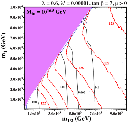
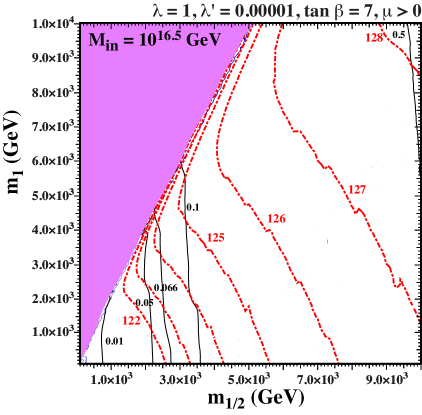
Figure 3: Examples of $(m_{1/2},m_{1})$ planes for $M_{\rm in}=10^{16.5}$ GeV when both Higgs 5-plets are twisted. All the modular weights $\alpha_{i}=\beta_{i}=0$, corresponding to $A_{t,b}=m_{1}$, $A_{\lambda}=2m_{3/2}$, $A_{\lambda^{\prime}}=0$, $B_{H}=2m_{1}$, and $B_{\Sigma}=0$. In both panels $\tan\beta=7$ and $\lambda^{\prime}=10^{-5}$ with $\lambda=0.6$ (left) and $\lambda=1$ (right). The shadings and contour colours are the same as in Fig. 1. The pink shaded region corresponds to parameter choices where the electroweak vacuum conditions cannot be satisfied, and radiative electroweak symmetry breaking is not possible.

Another very obvious difference between the left panel of Fig. 2 and Fig. 3 is the value of the proton lifetime. With $M_{\rm in}=M_{\rm GUT}$, the entire strip shown has a lifetime $\tau_{p}<10^{33}$ yrs, as it lies to the left of the contour labeled 0.01. However, the proton lifetime is significantly longer in both panels of Fig. 3, and there are acceptable parts of the relic density strip where $\tau_{p}>0.066\times 10^{35}$ yrs. Comparing the two panels allows one to see the effect of increasing $\lambda$ on the proton lifetime. For $\lambda=0.6$, the lifetime is sufficiently long for $m_{1/2}\gtrsim 5$ TeV, whereas for $\lambda=1$ this is relaxed to $m_{1/2}\gtrsim 2.5$ TeV. Increasing $\lambda$ much further is not possible due to its effect on the Yukawa couplings, as discussed in [19]. In both cases, the Higgs masses are reasonably consistent with 125 GeV, though due to the increased “bending” of the contours, the Higgs mass along the relic density strip is slightly lower for the larger value of $\lambda$ . The GM couplings are also acceptably small: in the GUT case shown in the left panel of Fig. 2 they are $\ll 1$ across the plane, whereas in Fig. 3 $c_{\Sigma}(m_{3/2}/m_{1/2})^{2}$ is of order 0.05 all along the relic density strip.

Since the strips with acceptable relic density in these models resemble the familiar focus-point region [48], one can expect that the spin-independent elastic scattering cross section on protons, $\sigma^{\rm SI}$, may be relatively large. Concentrating on the right panel of Fig. 3, we have computed $\sigma^{\rm SI}$ at two points: ($m_{1/2},m_{1}$) = (3100,6000) GeV and (4100, 8000) GeV. The resulting cross sections are $\sigma^{\rm SI}=(1.24\pm 0.77)\times 10^{-8}$ pb and $(1.90\pm 1.19)\times 10^{-9}$ pb with $m_{\chi}=930$ GeV and 1400 GeV, respectively, where we have assumed $\Sigma_{\pi N}=50\pm 8$ MeV [50] and $\sigma_{0}=36\pm 7$ MeV [51]. The central value for the former point is slightly above the recent LUX [52] and PandaX [53] bounds, but remains acceptable when uncertainties in the computed cross sections are taken into account. Furthermore, using nucleon matrix elements computed with lattice simulations as in [54] would reduce the predicted cross section by more than a factor 2 due to the smallness of strange-quark content in a nucleon. However, in both the cases studied one may anticipate a positive signal in upcoming direct detection experiments such as LUX-Zeplin and XENON1T/nT [55].

We consider next the case with the modular weights $\alpha_{t,b}=1$, $\alpha_{\lambda}=2$, $\alpha_{\lambda^{\prime}}=0$, $\beta_{H}=2$ and $\beta_{\Sigma}=0$, so that $A_{0}=B_{0}=0$ for all $A$ and $B$ terms. The right panel of Fig. 2 shows the $(m_{1/2},m_{1})$ plane for $M_{\rm in}=M_{\rm GUT}$, which is similar to that shown in the left panel when $A$ and $B$ terms are non-zero. The $A$ and $B$ terms are seen to affect somewhat the dependence on $m_{1}$ of the Higgs mass and the position of the relic density strip. The same case with $A_{0}=B_{0}=0$ but $M_{\rm in}=10^{16.5}$ GeV is shown in the left panel of Fig. 4. Comparing this with the right panel of Fig. 3, we see that the proton lifetime shows little dependence on $A_{0}$ and is similar in the two cases shown. For larger $M_{\rm in}=10^{18}$ GeV with $A_{0}=B_{0}=0$, as shown in the right panel of Fig. 4, we see that the relic density strip shifts to larger values of $m_{1}$ and the proton lifetime is somewhat longer. Much of the allowed dark matter strip has an acceptably long proton lifetime. The effect of adjusting the modular weights does not have a major effect on the elastic scattering cross section.

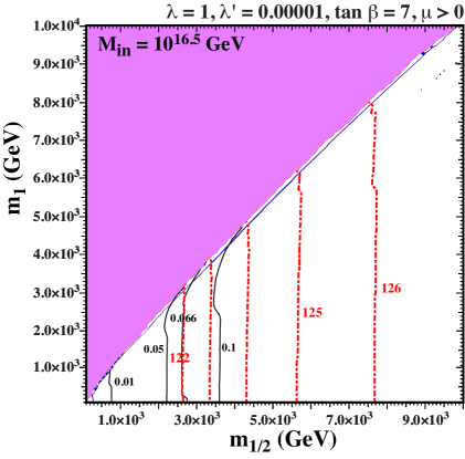
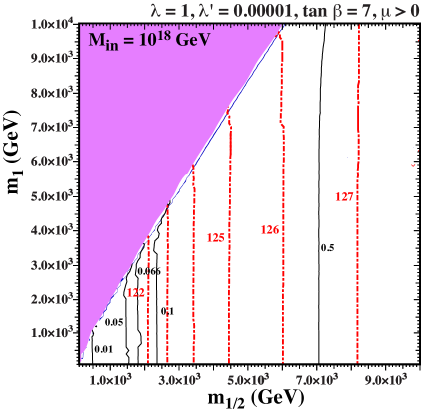
Figure 4: Examples of $(m_{1/2},m_{1})$ planes for $M_{\rm in}=10^{16.5}$ (left) and $10^{18}$ GeV (right) when both Higgs 5-plets are twisted. In both cases the modular weights are $\alpha_{t,b}=1$, $\alpha_{\lambda}=2$, $\alpha_{\lambda^{\prime}}=0$, $\beta_{H}=2$ and $\beta_{\Sigma}=0$, corresponding to $A_{0}=B_{0}=0$, and we assume $\tan\beta=7$, $\lambda=1$ and $\lambda^{\prime}=10^{-5}$. The shadings and contour colours are the same as in Fig. 1.

We consider next the case where only one of the Higgs 5-plets is twisted, so that

$$A_{\lambda}=(1-\alpha_{\lambda})m_{3/2}\qquad A_{\lambda^{\prime}}=-\alpha_{\lambda^{\prime}}m_{3/2}\qquad B_{H}=(1-\beta_{H})m_{3/2}\qquad B_{\Sigma}=-\beta_{\Sigma}m_{3/2}\,.$$ (30)

When $\overline{H}$ is twisted,

$$A_{t}=-\alpha_{t}m_{3/2}\qquad A_{b}=(1-\alpha_{b})m_{3/2}\,,$$ (31)

whereas when $H$ twisted,

$$A_{b}=-\alpha_{b}m_{3/2}\qquad A_{t}=(1-\alpha_{t})m_{3/2}\,.$$ (32)

Thus, in either case we have non-universal $A$-terms related via the Yukawa couplings.

We consider first the case with twisted $\overline{H}$. Examples of $(m_{1/2},m_{1})$ planes for $M_{\rm in}=10^{18}$ GeV are shown in Fig. 5. In both panels, we have taken $\tan\beta=7$, $\lambda=1$, and $\lambda^{\prime}=10^{-5}$. Since $H$ remains untwisted, we have $m_{0}=m_{2}=0$ and, since the two Higgs soft masses are unequal, this is an example of a super-GUT NUHM2 model [56, 46, 8, 9] . The region where one obtains an acceptable relic density could be expected from the upper left panel of Fig. 14 in [46], which shows an example of an $(m_{1},m_{2})$ plane for relatively low $m_{1/2}$, $m_{0}$ and $\tan\beta$. For $m_{2}=0$, we expect that there should be a funnel strip [6] where $s$-channel annihilation of the LSP through the heavy Higgs scalar and pseudoscalar dominates the total cross section and $m_{\chi}\approx m_{A}/2$. This generally occurs when $m_{1}^{2}<0$ at the input scale.

In the left panel of Fig. 5, we have taken $\alpha_{t}=0$, $\alpha_{b}=1$, $\alpha_{\lambda}=1$, $\alpha_{\lambda^{\prime}}=0$, $\beta_{H}=1$ and $\beta_{\Sigma}=0$, so that all the $A$ and $B$ terms vanish at the input scale. In the pink shaded region, the electroweak symmetry breaking (EWSB) conditions cannot be satisfied as $m_{A}^{2}<0$. Indeed, for $m_{1}^{2}<0$, we see a blue relic density strip above the shaded region. Whilst the proton lifetime is sufficiently large for $m_{1/2}\gtrsim 1.8$ TeV, the strip extends (barely visibly) to $m_{h}=123$ GeV (shown by the red dot-dashed contours). In the right panel of this figure, we have set all weights to zero, and therefore $A_{t}=0$, $A_{b}=m_{1}$, $A_{\lambda}=m_{1}$, $A_{\lambda^{\prime}}=0$, $B_{H}=m_{1}$, and $B_{\Sigma}=0$. Qualitatively, the two figures are very similar. The strip extends to slightly larger $m_{h}$ but, again, not much past 123 GeV. In both cases, $A_{t}=0$ at the input scale and, although $A_{b}\neq 0$ in the right panel, the dominant factor contributing to the Higgs mass is $A_{t}$. In both panels $c_{\Sigma}(m_{3/2}/m_{1/2})^{2}\approx-0.25$ in the allowed regions of the parameter space. We see that the proton lifetime is acceptably long when $m_{1/2}\gtrsim 1.7$ TeV along the dark matter strip. The elastic cross section near the end point of the relic density strip where $m_{1}\approx-3500$ GeV is quite small: $\sigma^{\rm SI}\approx 1\times 10^{-11}$ pb with $m_{\chi}\approx 800$ GeV, probably beyond the reach of LUX-Zeplin and XENON1T/nT [55], though still above the neutrino background level.

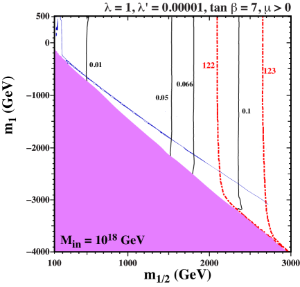
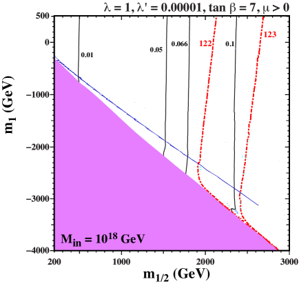
Figure 5: Examples of $(m_{1/2},m_{1})$ planes for $M_{\rm in}=10^{18}$ GeV when only $\overline{H}$ is twisted. In the left panel, the modular weights are $\alpha_{t}=0$, $\alpha_{b}=1$, $\alpha_{\lambda}=1$, $\alpha_{\lambda^{\prime}}=0$, $\beta_{H}=1$ and $\beta_{\Sigma}=0$, so that all trilinear and bilinear terms vanish. In the right panel, all the weights vanish, so that $A_{t}=0$, $A_{b}=m_{1}$, $A_{\lambda}=m_{1}$, $A_{\lambda^{\prime}}=0$, $B_{H}=m_{1}$, and $B_{\Sigma}=0$. In both panels $\tan\beta=7$, $\lambda=1$ and $\lambda^{\prime}=10^{-5}$. The shadings and contour colours are the same as in Fig. 1.

The Higgs mass can be increased slightly by turning on the weight $\alpha_{t}$ controlling $A_{t}$. To determine the optimal value for $\alpha_{t}$, for all other $A_{i}=0$ and $B_{i}=0$, we scan over $\alpha_{t}$. In the left panel of Fig. 6 the resulting $(A_{t},m_{1/2})$ plane for fixed $m_{1}=-3000$ GeV and $m_{0}=m_{2}=0$ is shown. Once again, the pink shaded region is excluded as $m_{A}^{2}<0$ and the constraints for electroweak symmetry breaking cannot be satisfied. The blue line (enhanced here for visibility) shows the position of the relic density funnel strip. We see that the largest value of the Higgs mass obtained is slightly larger than 124 GeV, which is reached when $A_{t}/|m_{1}|\sim 1$. The proton lifetime is acceptably long for $m_{1/2}\gtrsim 1.8$ TeV along the dark matter strip, and the GM coupling shown by the green lines is $\gtrsim-1.5$ in this region. In the right panel, we show the corresponding $(m_{1/2},m_{1})$ plane with $A_{t}=m_{1}$ and again all other $A_{i}=B_{i}=0$. Here we see that the funnel strip extends to Higgs masses slightly larger than 124 GeV, where the proton lifetime is about $10^{34}$ yrs. Points along the dark matter strip with $m_{1/2}\gtrsim 1.7$ TeV have an acceptably long proton lifetime. In both cases, displayed, the elastic cross sections are relatively small. Near the end point of the relic density strip where $m_{1}\approx-3000$ GeV, we find $\sigma^{\rm SI}\approx 2\times 10^{-11}$ pb with $m_{\chi}\approx 950$ GeV. Although this cross section is still above the neutrino background, it may be difficult to detect in the planned LUX-Zeplin and XENON1T/nT experiments.

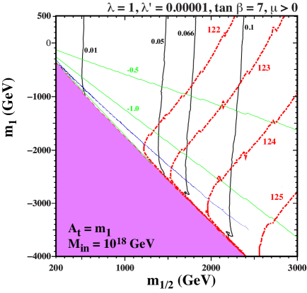
Figure 6: Left panel: The $(A_{t},m_{1/2})$ plane for $\tan\beta=7,\lambda=1$ and $\lambda^{\prime}=10^{-5}$ with $M_{\rm in}=10^{18}$ GeV, $m_{0}=0$ and $m_{1}=-3000$ GeV when only $\overline{H}$ is twisted. Right panel: The corresponding $(m_{1/2},m_{1})$ plane. Here, the modular weights are $\alpha_{b}=1$, $\alpha_{\lambda}=1$, $\alpha_{\lambda^{\prime}}=0$, $\beta_{H}=1$ and $\beta_{\Sigma}=0$. For the left panel $\alpha_{t}$ varies and $m_{1}$ is fixed while for the right panel $A_{t}=m_{1}$ ($\alpha_{t}=-1$) and all other $A_{i}=B_{i}=0$. The shadings and contour colours are the same as in Fig. 1.

Finally, we consider the effects of twisting $H$ leaving $\overline{H}$ untwisted. In this case, $m_{0}=m_{1}=0$, and previous studies lead us to expect the relic density strip to lie at positive values of $m_{2}^{2}$. Once again, we have taken $\tan\beta=7$, $\lambda=1$, and $\lambda^{\prime}=10^{-5}$. In the left panel of Fig. 7, we have taken $\alpha_{t}=1$, $\alpha_{b}=0$, $\alpha_{\lambda}=1$, $\alpha_{\lambda^{\prime}}=0$, $\beta_{H}=1$ and $\beta_{\Sigma}=0$, so that all $A$ and $B$ terms vanish at the input scale. In the pink shaded region, the EWSB conditions cannot be satisfied, but in this case it is because $\mu^{2}<0$. Just to the right of the excluded region, we see the equivalent of the focus-point strip, where the LSP is mostly Higgsino. Still further to the right, we see two closely-spaced strips corresponding to the funnel region with a mostly bino-like LSP. For this choice of $\lambda$ and $\lambda^{\prime}$, the proton lifetime is sufficiently long if $m_{1/2}\gtrsim 1.8$ TeV, but the Higgs mass is $\lesssim 123$ GeV unless $m_{1/2}\gtrsim 2.7$ TeV. In the right panel of Fig. 7, we again take all weights equal to 0, so that $A_{t}=m_{2}$, $A_{b}=0$, $A_{\lambda}=m_{2}$, $A_{\lambda^{\prime}}=0$, $B_{H}=m_{2}$, and $B_{\Sigma}=0$. In this case, the pink shaded region has $m_{A}^{2}<0$ and we see the funnel strip running to values of $m_{h}>125$ GeV. Comparing this with the left panel, we see the effect of the non-zero value of $A_{t}$ on $m_{h}$. In both panels we see that points along the dark matter strips with $m_{1/2}\gtrsim 1.7$ TeV have an acceptably long proton lifetime.

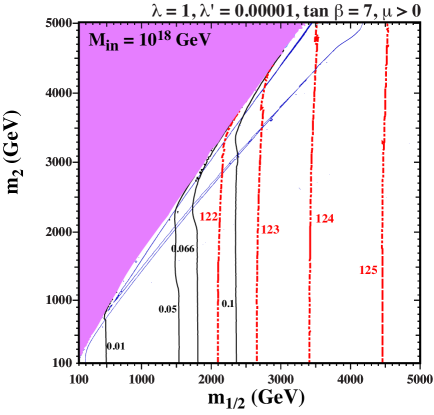
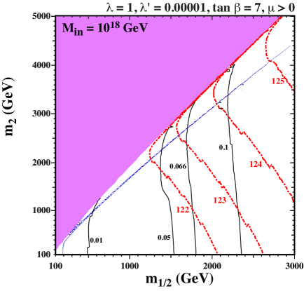
Figure 7: Examples of $(m_{1/2},m_{2})$ planes for $M_{\rm in}=10^{18}$ when only $H$ is twisted. In the left panel, all trilinear and bilinear terms are zero. The modular weights are $\alpha_{t}=1$, $\alpha_{b}=0$, $\alpha_{\lambda}=1$, $\alpha_{\lambda^{\prime}}=0$, $\beta_{H}=1$ and $\beta_{\Sigma}=0$, corresponding to $A_{0}=B_{0}=0$. In the right panel, all weights are zero, so that $A_{t}=m_{2}$, $A_{b}=0$, $A_{\lambda}=m_{2}$, $A_{\lambda^{\prime}}=0$, $B_{H}=m_{2}$, and $B_{\Sigma}=0$. In both panels $\tan\beta=7$, $\lambda=1$ and $\lambda^{\prime}=10^{-5}$. The shadings and contour colours are the same as in Fig. 1.

Since we have both a focus point strip and a funnel region, there is more variation in the computed elastic cross section. Corresponding to the left panel of Fig. 7, we considered points at $m_{2}=4000$ GeV with $m_{1/2}\simeq 2700$ GeV (focus point with $m_{\chi}\simeq 900$ GeV) and $m_{1/2}\simeq 3200$ GeV (funnel with $m_{\chi}\simeq 1160$ GeV). We found $\sigma^{\rm SI}\simeq(2.2\pm 1.4)\times 10^{-8}$ pb and $(1.2\pm 0.7)\times 10^{-10}$ pb respectively. At higher $m_{0}=5000$ GeV, the cross section on the focus point at $m_{1/2}\simeq 1065$ GeV drops to $(6.4\pm 4.0)\times 10^{-9}$ pb and on the funnel at $m_{1/2}\simeq 1530$ GeV drops to $(7.2\pm 4.5)\times 10^{-11}$ pb. When the weights are set to zero as in the right panel of Fig. 7, we have only a funnel strip and the cross section is quite low. For $(m_{1/2},m_{2})$ = (1920,3000), we find $\sigma^{\rm SI}\simeq(5.3\pm 3.3)\times 10^{-11}$ pb and for $(m_{1/2},m_{2})$ = (2965,4400), we find $\sigma^{\rm SI}=(2.2\pm 1.4)\times 10^{-11}$ pb.

4 Discussion

We have shown in this paper that, if the matter and Higgs supermultiplets are all untwisted, super-GUT SU(5) models are unable to provide simultaneously a long enough proton lifetime, a small enough relic LSP density and an acceptable Higgs mass in the framework of no-scale supergravity, even in the presence of a Giudice-Masiero term in the Kähler potential. However, all of these phenomenological requirements can be reconciled if one or both of the GUT Higgs fiveplets is twisted. We have exhibited satisfactory solutions for various values of the input super-GUT scale $M_{\rm in}$, the GUT Yukawa couplings that are important in the RGEs above the GUT scale, and the modular weights of the various matter and Higgs fields. All the examples shown assume $\tan\beta=7$: significantly smaller values of $\tan\beta$ are largely excluded because $m_{h}$ is too small, and significantly larger values of $\tan\beta$ are largely excluded because the proton lifetime is too short. Spin-independent dark matter scattering may be observable in some of the cases studied.

Although, as we have shown, many of the problems of the minimal SU(5) GUT model may be resolved in the no-scale SU(5) super-GUT, including rapid proton decay through dimension-5 operators, in a manner compatible with the dark matter density and the Higgs mass, other issues such as neutrino masses/oscillations remain unresolved. Moreover, the resolution of the minimal supersymmetric SU(5) GUT problems within the super-GUT and no-scale supergravity frameworks is quite constrained and somewhat contrived. It also remains unclear how an SU(5) GUT model could be embedded within string theory.

A natural alternative is the flipped SU(5)$\times$U(1) framework proposed in [57, 58, 59], which resolves automatically the problems mentioned above, and can be embedded with string theory. Choosing even the simplest strict no-scale boundary conditions $m_{0}=A_{0}=B_{0}=0$ at $M_{in}$ provides a very interesting flipped SU(5) framework that satisfies all the constraints from present low-energy phenomenology, including the relic dark matter density and the proton lifetime, and makes interesting predictions for Run 2 of the LHC [60]. Moreover, flipped SU(5) also contains a rationale for $M_{in}>M_{GUT}$, since the final unification of the SU(5) and U(1) gauge couplings could well occur at the string scale. We therefore plan to consider the possibility of a no-scale flipped SU(5) super-GUT in a forthcoming paper.

References

- [1] H. Georgi and S. L. Glashow, Phys. Rev. Lett. 32 (1974) 438 doi:10.1103/PhysRevLett.32.438.
- [2] S. Dimopoulos and H. Georgi, Nucl. Phys. B 193, 150 (1981); N. Sakai, Z. Phys. C 11, 153 (1981).
- [3] E. Cremmer, S. Ferrara, C. Kounnas and D. V. Nanopoulos, Phys. Lett. 133B (1983) 61 doi:10.1016/0370-2693(83)90106-5; J. R. Ellis, A. B. Lahanas, D. V. Nanopoulos and K. Tamvakis, Phys. Lett. 134B (1984) 429 doi:10.1016/0370-2693(84)91378-9; J. R. Ellis, C. Kounnas and D. V. Nanopoulos, Nucl. Phys. B 247 (1984) 373 doi:10.1016/0550-3213(84)90555-8; A. B. Lahanas and D. V. Nanopoulos, Phys. Rept. 145 (1987) 1 doi:10.1016/0370-1573(87)90034-2.
- [4] E. Witten, Phys. Lett. B 155 (1985) 151.
- [5] J. Ellis, D. V. Nanopoulos and K. A. Olive, Phys. Rev. Lett. 111 (2013) 111301 Erratum: [Phys. Rev. Lett. 111 (2013) 129902] doi:10.1103/PhysRevLett.111.129902, 10.1103/PhysRevLett.111.111301 [arXiv:1305.1247 [hep-th]]; J. Ellis, M. A. G. Garcia, D. V. Nanopoulos and K. A. Olive, Class. Quant. Grav. 33 (2016) 094001 doi:10.1088/0264-9381/33/9/094001 [arXiv:1507.02308 [hep-ph]].
- [6] M. Drees and M. M. Nojiri, Phys. Rev. D 47 (1993) 376 [arXiv:hep-ph/9207234]; H. Baer and M. Brhlik, Phys. Rev. D 53 (1996) 597 [arXiv:hep-ph/9508321]; Phys. Rev. D 57 (1998) 567 [arXiv:hep-ph/9706509]; H. Baer, M. Brhlik, M. A. Diaz, J. Ferrandis, P. Mercadante, P. Quintana and X. Tata, Phys. Rev. D 63 (2001) 015007 [arXiv:hep-ph/0005027]; J. R. Ellis, T. Falk, G. Ganis, K. A. Olive and M. Srednicki, Phys. Lett. B 510 (2001) 236 [arXiv:hep-ph/0102098].
- [7] G. L. Kane, C. F. Kolda, L. Roszkowski and J. D. Wells, Phys. Rev. D 49 (1994) 6173 [arXiv:hep-ph/9312272]; J. R. Ellis, T. Falk, K. A. Olive and M. Schmitt, Phys. Lett. B 388 (1996) 97 [arXiv:hep-ph/9607292]; Phys. Lett. B 413 (1997) 355 [arXiv:hep-ph/9705444]; V. D. Barger and C. Kao, Phys. Rev. D 57 (1998) 3131 [arXiv:hep-ph/9704403]; L. Roszkowski, R. Ruiz de Austri and T. Nihei, JHEP 0108 (2001) 024 [arXiv:hep-ph/0106334]; A. Djouadi, M. Drees and J. L. Kneur, JHEP 0108 (2001) 055 [arXiv:hep-ph/0107316]; U. Chattopadhyay, A. Corsetti and P. Nath, Phys. Rev. D 66 (2002) 035003 [arXiv:hep-ph/0201001]; J. R. Ellis, K. A. Olive and Y. Santoso, New Jour. Phys. 4 (2002) 32 [arXiv:hep-ph/0202110]; H. Baer, C. Balazs, A. Belyaev, J. K. Mizukoshi, X. Tata and Y. Wang, JHEP 0207 (2002) 050 [arXiv:hep-ph/0205325]; R. Arnowitt and B. Dutta, arXiv:hep-ph/0211417; J. R. Ellis, T. Falk, G. Ganis, K. A. Olive and M. Schmitt, Phys. Rev. D 58 (1998) 095002 [arXiv:hep-ph/9801445]; J. R. Ellis, T. Falk, G. Ganis and K. A. Olive, Phys. Rev. D 62 (2000) 075010 [arXiv:hep-ph/0004169]; J. R. Ellis, K. A. Olive, Y. Santoso and V. C. Spanos, Phys. Lett. B 565 (2003) 176 [arXiv:hep-ph/0303043]; H. Baer and C. Balazs, JCAP 0305, 006 (2003) [arXiv:hep-ph/0303114]; A. B. Lahanas and D. V. Nanopoulos, Phys. Lett. B 568, 55 (2003) [arXiv:hep-ph/0303130]; U. Chattopadhyay, A. Corsetti and P. Nath, Phys. Rev. D 68, 035005 (2003) [arXiv:hep-ph/0303201]; C. Munoz, Int. J. Mod. Phys. A 19, 3093 (2004) [arXiv:hep-ph/0309346]; R. Arnowitt, B. Dutta and B. Hu, arXiv:hep-ph/0310103; J. Ellis and K. A. Olive, arXiv:1001.3651 [astro-ph.CO], published in Particle dark matter, ed. G. Bertone, pp. 142-163; J. Ellis and K. A. Olive, Eur. Phys. J. C 72, 2005 (2012) [arXiv:1202.3262 [hep-ph]]; O. Buchmueller et al., Eur. Phys. J. C 74 (2014) 3, 2809 [arXiv:1312.5233 [hep-ph]].
- [8] J. Ellis, F. Luo, K. A. Olive and P. Sandick, Eur. Phys. J. C 73, no. 4, 2403 (2013) [arXiv:1212.4476 [hep-ph]].
- [9] J. Ellis, J. L. Evans, F. Luo, N. Nagata, K. A. Olive and P. Sandick, Eur. Phys. J. C 76, no. 1, 8 (2016) doi:10.1140/epjc/s10052-015-3842-6 [arXiv:1509.08838 [hep-ph]].
- [10] R. Barbieri, S. Ferrara and C. A. Savoy, Phys. Lett. B 119, 343 (1982).
- [11] J. R. Ellis, K. A. Olive, Y. Santoso and V. C. Spanos, Phys. Lett. B 573 (2003) 162 [arXiv:hep-ph/0305212], and Phys. Rev. D 70 (2004) 055005 [arXiv:hep-ph/0405110].
- [12] M. Ibe, T. Moroi and T. T. Yanagida, Phys. Lett. B 644, 355 (2007) [hep-ph/0610277]; M. Ibe and T. T. Yanagida, Phys. Lett. B 709, 374 (2012) [arXiv:1112.2462 [hep-ph]]; M. Ibe, S. Matsumoto and T. T. Yanagida, Phys. Rev. D 85, 095011 (2012) [arXiv:1202.2253 [hep-ph]]; J. L. Evans, M. Ibe, K. A. Olive and T. T. Yanagida, Phys. Rev. D 91, 055008 (2015) doi:10.1103/PhysRevD.91.055008 [arXiv:1412.3403 [hep-ph]].
- [13] J. L. Evans, M. Ibe, K. A. Olive and T. T. Yanagida, Eur. Phys. J. C 73, 2468 (2013) doi:10.1140/epjc/s10052-013-2468-9 [arXiv:1302.5346 [hep-ph]].
- [14] J. L. Evans, K. A. Olive, M. Ibe and T. T. Yanagida, Eur. Phys. J. C 73, no. 10, 2611 (2013) doi:10.1140/epjc/s10052-013-2611-7 [arXiv:1305.7461 [hep-ph]].
- [15] G. F. Giudice and A. Masiero, Phys. Lett. B 206, 480 (1988).
- [16] M. Dine and D. MacIntire, Phys. Rev. D 46, 2594 (1992) [hep-ph/9205227]; L. Randall and R. Sundrum, Nucl. Phys. B 557, 79 (1999) [arXiv:hep-th/9810155]; G. F. Giudice, M. A. Luty, H. Murayama and R. Rattazzi, JHEP 9812, 027 (1998) [arXiv:hep-ph/9810442]; J. A. Bagger, T. Moroi and E. Poppitz, JHEP 0004, 009 (2000) [arXiv:hep-th/9911029]; P. Binetruy, M. K. Gaillard and B. D. Nelson, Nucl. Phys. B 604, 32 (2001) [arXiv:hep-ph/0011081].
- [17] J. R. Ellis, K. A. Olive and P. Sandick, Phys. Lett. B 642, 389 (2006) [hep-ph/0607002]; J. R. Ellis, K. A. Olive and P. Sandick, JHEP 0706, 079 (2007) [arXiv:0704.3446 [hep-ph]]; J. R. Ellis, K. A. Olive and P. Sandick, JHEP 0808, 013 (2008) [arXiv:0801.1651 [hep-ph]].
- [18] J. Ellis, A. Mustafayev and K. A. Olive, Eur. Phys. J. C 69 (2010) 201 doi:10.1140/epjc/s10052-010-1373-8 [arXiv:1003.3677 [hep-ph]].
- [19] J. Ellis, J. L. Evans, A. Mustafayev, N. Nagata and K. A. Olive, Eur. Phys. J. C 76, 592 (2016) doi:10.1140/epjc/s10052-016-4437-6 [arXiv:1608.05370 [hep-ph]].
- [20] J. Ellis, A. Mustafayev and K. A. Olive, Eur. Phys. J. C 69, 219 (2010) [arXiv:1004.5399 [hep-ph]].
- [21] J. R. Ellis, D. V. Nanopoulos and K. A. Olive, Phys. Lett. B 525, 308 (2002) [arXiv:hep-ph/0109288].
- [22] J. Ellis, M. A. G. Garcia, D. V. Nanopoulos and K. A. Olive, JCAP 1510, no. 10, 003 (2015) doi:10.1088/1475-7516/2015/10/003 [arXiv:1503.08867 [hep-ph]].
- [23] K. Choi, A. Falkowski, H. P. Nilles and M. Olechowski, Nucl. Phys. B 718, 113 (2005) [hep-th/0503216]; O. Lebedev, H. P. Nilles and M. Ratz, Phys. Lett. B 636, 126 (2006) [hep-th/0603047]; O. Lebedev, V. Lowen, Y. Mambrini, H. P. Nilles and M. Ratz, JHEP 0702, 063 (2007) [hep-ph/0612035].
- [24] J. L. Evans, N. Nagata and K. A. Olive, Phys. Rev. D 91, 055027 (2015) doi:10.1103/PhysRevD.91.055027 [arXiv:1502.00034 [hep-ph]].
- [25] E. Dudas, Y. Mambrini, A. Mustafayev and K. A. Olive, Eur. Phys. J. C 72, 2138 (2012) [Eur. Phys. J. C 73, 2430 (2013)] [arXiv:1205.5988 [hep-ph]]; E. Dudas, A. Linde, Y. Mambrini, A. Mustafayev and K. A. Olive, Eur. Phys. J. C 73, no. 1, 2268 (2013) [arXiv:1209.0499 [hep-ph]].
- [26] N. Polonsky and A. Pomarol, Phys. Rev. Lett. 73, 2292 (1994) [arXiv:hep-ph/9406224]; Phys. Rev. D 51 (1995) 6532 [arXiv:hep-ph/9410231].
- [27] H. Baer, M. A. Diaz, P. Quintana and X. Tata, JHEP 0004, 016 (2000) [arXiv:hep-ph/0002245].
- [28] J. Ellis, A. Mustafayev and K. A. Olive, Eur. Phys. J. C 71, 1689 (2011) [arXiv:1103.5140 [hep-ph]].
- [29] J. Hisano, H. Murayama and T. Yanagida, Phys. Rev. Lett. 69, 1014 (1992).
- [30] J. Hisano, H. Murayama and T. Yanagida, Nucl. Phys. B 402, 46 (1993) [hep-ph/9207279].
- [31] J. Hisano, T. Kuwahara and N. Nagata, Phys. Lett. B 723, 324 (2013) [arXiv:1304.0343 [hep-ph]].
- [32] J. R. Ellis, K. Enqvist, D. V. Nanopoulos and K. Tamvakis, Phys. Lett. B 155, 381 (1985).
- [33] C. T. Hill, Phys. Lett. B 135, 47 (1984); Q. Shafi and C. Wetterich, Phys. Rev. Lett. 52, 875 (1984); M. Drees, Phys. Lett. B 158, 409 (1985); M. Drees, Phys. Rev. D 33, 1468 (1986).
- [34] K. Tobe and J. D. Wells, Phys. Lett. B 588, 99 (2004) [hep-ph/0312159].
- [35] J. Hisano, H. Murayama and T. Goto, Phys. Rev. D 49, 1446 (1994).
- [36] F. Borzumati and T. Yamashita, Prog. Theor. Phys. 124, 761 (2010) [arXiv:0903.2793 [hep-ph]].
- [37] Y. Kawamura, H. Murayama and M. Yamaguchi, Phys. Rev. D 51, 1337 (1995) [hep-ph/9406245].
- [38] V. D. Barger, M. S. Berger and P. Ohmann, Phys. Rev. D 49 (1994) 4908 [arXiv:hep-ph/9311269]; W. de Boer, R. Ehret and D. I. Kazakov, Z. Phys. C 67 (1995) 647 [arXiv:hep-ph/9405342]; M. Carena, J. R. Ellis, A. Pilaftsis and C. E. Wagner, Nucl. Phys. B 625 (2002) 345 [arXiv:hep-ph/0111245].
- [39] M. Schmaltz and W. Skiba, Phys. Rev. D 62, 095005 (2000) [arXiv:hep-ph/0001172]; M. Schmaltz and W. Skiba, Phys. Rev. D 62, 095004 (2000) [arXiv:hep-ph/0004210].
- [40] J. Ellis, K. Olive and L. Velasco-Sevilla, Eur. Phys. J. C 76, no. 10, 562 (2016) doi:10.1140/epjc/s10052-016-4398-9 [arXiv:1605.01398 [hep-ph]].
- [41] T. Hahn, S. Heinemeyer, W. Hollik, H. Rzehak and G. Weiglein, Phys. Rev. Lett. 112 (2014) 14, 141801 [arXiv:1312.4937 [hep-ph]].
- [42] J. Hisano, D. Kobayashi, T. Kuwahara and N. Nagata, JHEP 1307, 038 (2013) [arXiv:1304.3651 [hep-ph]]; N. Nagata and S. Shirai, JHEP 1403, 049 (2014) [arXiv:1312.7854 [hep-ph]].
- [43] J. R. Ellis, M. K. Gaillard and D. V. Nanopoulos, Phys. Lett. B 88, 320 (1979).
- [44] V. Takhistov [Super-Kamiokande Collaboration], arXiv:1605.03235 [hep-ex]; K. Abe et al. [Super-Kamiokande Collaboration], Phys. Rev. D 90, no. 7, 072005 (2014) [arXiv:1408.1195 [hep-ex]].
- [45] H. Baer, A. Mustafayev, S. Profumo, A. Belyaev and X. Tata, Phys. Rev. D 71 (2005) 095008 [arXiv:hep-ph/0412059]; H. Baer, A. Mustafayev, S. Profumo, A. Belyaev and X. Tata, JHEP 0507 (2005) 065, hep-ph/0504001.
- [46] J. R. Ellis, K. A. Olive and P. Sandick, Phys. Rev. D 78 (2008) 075012 [arXiv:0805.2343 [hep-ph]].
- [47] J. Ellis, T. Falk, and K.A. Olive, Phys. Lett. B444 (1998) 367 [arXiv:hep-ph/9810360]; J. Ellis, T. Falk, K.A. Olive, and M. Srednicki, Astr. Part. Phys. 13 (2000) 181 [Erratum-ibid. 15 (2001) 413] [arXiv:hep-ph/9905481]; R. Arnowitt, B. Dutta and Y. Santoso, Nucl. Phys. B 606 (2001) 59 [arXiv:hep-ph/0102181]; M. E. Gómez, G. Lazarides and C. Pallis, Phys. Rev. D D61 (2000) 123512 [arXiv:hep-ph/9907261]; Phys. Lett. B487 (2000) 313 [arXiv:hep-ph/0004028]; Nucl. Phys. B B638 (2002) 165 [arXiv:hep-ph/0203131]; T. Nihei, L. Roszkowski and R. Ruiz de Austri, JHEP 0207 (2002) 024 [arXiv:hep-ph/0206266]; M. Citron, J. Ellis, F. Luo, J. Marrouche, K. A. Olive and K. J. de Vries, Phys. Rev. D 87, 036012 (2013) [arXiv:1212.2886 [hep-ph]].
- [48] J. L. Feng, K. T. Matchev and T. Moroi, Phys. Rev. Lett. 84, 2322 (2000) [arXiv:hep-ph/9908309]; Phys. Rev. D 61, 075005 (2000) [arXiv:hep-ph/9909334]; J. L. Feng, K. T. Matchev and F. Wilczek, Phys. Lett. B 482, 388 (2000) [arXiv:hep-ph/0004043]; H. Baer, T. Krupovnickas, S. Profumo and P. Ullio, JHEP 0510 (2005) 020 [hep-ph/0507282]; J. L. Feng, K. T. Matchev and D. Sanford, Phys. Rev. D 85, 075007 (2012) [arXiv:1112.3021 [hep-ph]]; P. Draper, J. Feng, P. Kant, S. Profumo and D. Sanford, Phys. Rev. D 88, 015025 (2013) [arXiv:1304.1159 [hep-ph]].
- [49] L. Calibbi, Y. Mambrini and S. K. Vempati, JHEP 0709, 081 (2007) [arXiv:0704.3518 [hep-ph]]; L. Calibbi, A. Faccia, A. Masiero and S. K. Vempati, Phys. Rev. D 74, 116002 (2006) [arXiv:hep-ph/0605139]; E. Carquin, J. Ellis, M. E. Gomez, S. Lola and J. Rodriguez-Quintero, JHEP 0905 (2009) 026 [arXiv:0812.4243 [hep-ph]].
- [50] J. R. Ellis, K. A. Olive and C. Savage, Phys. Rev. D 77, 065026 (2008) doi:10.1103/PhysRevD.77.065026 [arXiv:0801.3656 [hep-ph]].
- [51] B. Borasoy and U. G. Meissner, Annals Phys. 254, 192 (1997) doi:10.1006/aphy.1996.5630 [hep-ph/9607432].
- [52] D. S. Akerib et al. [LUX Collaboration], Phys. Rev. Lett. 118, no. 2, 021303 (2017) doi:10.1103/PhysRevLett.118.021303 [arXiv:1608.07648 [astro-ph.CO]].
- [53] A. Tan et al. [PandaX-II Collaboration], Phys. Rev. Lett. 117, no. 12, 121303 (2016) [arXiv:1607.07400 [hep-ex]].
- [54] A. Abdel-Rehim et al. [ETM Collaboration], Phys. Rev. Lett. 116, no. 25, 252001 (2016) doi:10.1103/PhysRevLett.116.252001 [arXiv:1601.01624 [hep-lat]].
- [55] D. C. Malling et al., arXiv:1110.0103 [astro-ph.IM]; E. Aprile et al. [XENON Collaboration], JCAP 1604 (2016), 027 [arXiv:1512.07501 [physics.ins-det]].
- [56] J. Ellis, K. Olive and Y. Santoso, Phys. Lett. B 539, 107 (2002) [arXiv:hep-ph/0204192]; J. R. Ellis, T. Falk, K. A. Olive and Y. Santoso, Nucl. Phys. B 652, 259 (2003) [arXiv:hep-ph/0210205].
- [57] S. M. Barr, Phys. Lett. 112B (1982) 219 doi:10.1016/0370-2693(82)90966-2.
- [58] J. P. Derendinger, J. E. Kim and D. V. Nanopoulos, Phys. Lett. 139B (1984) 170 doi:10.1016/0370-2693(84)91238-3.
- [59] I. Antoniadis, J. R. Ellis, J. S. Hagelin and D. V. Nanopoulos, Phys. Lett. B 194 (1987) 231 doi:10.1016/0370-2693(87)90533-8; Phys. Lett. B 205 (1988) 459 doi:10.1016/0370-2693(88)90978-1; Phys. Lett. B 208 (1988) 209 Addendum: [Phys. Lett. B 213 (1988) 562] doi:10.1016/0370-2693(88)90419-4; Phys. Lett. B 231 (1989) 65 doi:10.1016/0370-2693(89)90115-9.
- [60] T. Li, J. A. Maxin, D. V. Nanopoulos and J. W. Walker, Phys. Rev. D 83, 056015 (2011) doi:10.1103/PhysRevD.83.056015 [arXiv:1007.5100 [hep-ph]]; Phys. Lett. B 710, 207 (2012) doi:10.1016/j.physletb.2012.02.086 [arXiv:1112.3024 [hep-ph]]; Phys. Rev. D 84, 076003 (2011) doi:10.1103/PhysRevD.84.076003 [arXiv:1103.4160 [hep-ph]]; T. Li, J. A. Maxin and D. V. Nanopoulos, Phys. Lett. B 764, 167 (2017) doi:10.1016/j.physletb.2016.11.022 [arXiv:1609.06294 [hep-ph]].