Enhanced conservation properties of Vlasov codes through coupling with conservative fluid models

Abstract

Many phenomena in collisionless plasma physics require a kinetic description. The evolution of the phase space density can be modeled by means of the Vlasov equation, which has to be solved numerically in most of the relevant cases. One of the problems that often arise in such simulations is the violation of important physical conservation laws. Numerical diffusion in phase space translates into unphysical heating, which can increase the overall energy significantly, depending on the time scale and the plasma regime. In this paper, a general and straightforward way of improving conservation properties of Vlasov schemes is presented that can potentially be applied to a variety of different codes. The basic idea is to use fluid models with good conservation properties for correcting kinetic models. The higher moments that are missing in the fluid models are provided by the kinetic codes, so that both kinetic and fluid codes compensate the weaknesses of each other in a closed feedback loop.

1 Introduction

There is a variety of different plasma models with different strengths and weaknesses. For collisionless plasmas, the Vlasov equation is pretty accurate from a physical point of view, but it is typically hard to solve analytically and expensive when it comes to numerical simulations. Besides issues with reaching a reasonable resolution, numerical Vlasov codes typically suffer from certain problems like recurrence or artificial heating that are due to the discretization of the phase space. The latter problem destroys energy conservation and is thus highly unphysical. Fluid models only describe the evolution of the (lowest) moments of the phase space density and are thus much easier to handle than the full kinetic models, both analytically and numerically. Here, the main problem lies in the fact that the equations for the moments build an infinite hierarchy of dependent expressions. While the hierarchy as a whole is still exact, only the lowest moments can be examined in practice and approximating closures determine the behavior of the final system of equations to a large degree. Besides that, certain conservation properties are easy to guarantee in numerical fluid codes.

At this point it becomes clear that kinetic and fluid models complement each other: kinetic models offer higher moments and lack certain conservation properties, while fluid models need information on higher moments and have good conservation properties for the lower moments. On the basis of this and taking into account that the numerical costs of fluid models are negligible compared to those of kinetic models, the basic idea is to use fluid codes alongside kinetic codes in simulations and feed each of the codes information from the other one in order to improve the overall results. The situation can be imagined as follows: Two simulations of the same physical problem with different models run parallely and mostly independent of each other, but in each step the fluid code gets prescribed higher moments as a closure from the kinetic code and the phase space density is adapted to the moments given by the fluid model. The adaption or fitting of the phase space density is done through a linear transformation of the velocity space that is a generalization of the concept introduced in [1]. There, this fitting was used for coupling kinetic and fluid codes in different regions, but the idea stays the same. The generalized version of the fitting procedure can handle non-isotropic temperatures and may also be used for coupling of fluid and kinetic codes between separated regions, an area which is of major importance in fluid and plasma theory (see e.g. [2, 3, 4, 5, 6, 7, 8, 9, 10, 11, 12]).

This paper is organized as follows: In 2, the underlying physical equations and definitions are summarized in order to clarify the general setup and for later reference. The numerical schemes that are used for solving these equations are briefly described in 3. After that, the fitting procedure that is used for correcting the phase space density on the basis of its moments is presented in 4. Various tests of the correction procedure are discussed in 5. Finally, a summary of the results and an outlook are given in 6.

2 Physical models

The focus of the present paper lies on classical, non-relativistic, collisionless electron/ion plasmas. Such plasmas can be described in terms of the phase space densities $f_{s}(\textbf{x},\textbf{v},t)$, where the subscript $s$ may be replaced by $e$ for electrons or $i$ for ions. Each $f_{s}$ is governed by the non-relativistic Vlasov equation

$$\partial_{t}f_{s}+\textbf{v}\cdot\nabla_{\textbf{x}}f_{s}+\frac{q_{s}}{m_{s}}\big{(}\textbf{E}+\textbf{v}\times\textbf{B}\big{)}\cdot\nabla_{\textbf{v}}f_{s}=0,$$ (1)

where $q_{s}$ is the charge of a particle of species $s$ and $m_{s}$ is its charge. A closure for the electric field E and the magnetic field B is given by Maxwell’s equations:

$$\nabla\cdot\textbf{E} =\frac{\rho}{\varepsilon_{0}}$$ (2a)

$$\nabla\cdot\textbf{B} =0$$ (2b)

$$\partial_{t}\textbf{B} =-\nabla\times\textbf{E}$$ (2c)

$$\partial_{t}\textbf{E} =c^{2}\left(\nabla\times\textbf{B}-\mu_{0}\textbf{J}\right)$$ (2d)

Charge density $\rho$ and current density J, however, depend on $f_{e}$ and $f_{i}$. They are defined as:

$$\rho :=\sum_{s}q_{s}\int f_{s}\mathrm{d}\textbf{v},$$ (3a)

J $$:=\sum_{s}q_{s}\int\textbf{v}f_{s}\mathrm{d}\textbf{v}.$$ (3b)

Even though (1) offers a comprehensive description of the plasmas under consideration, solving it may be very challenging and the full phase space density is not always of interest, anyway. Thus, it is possible to consider the moments $\mu_{n,s}$ of $f_{s}$, instead,

$$\mu_{n,s}:=\int\textbf{v}^{n}f_{s}\mathrm{d}\textbf{v}.$$ (4)

The lowest moments that are relevant for the subsequent discussion are given separate names:

particle density: $$n_{s} :=\mu_{0,s}=\int f_{s}\mathrm{d}v$$ (5a)

bulk velocity: $$\textbf{u}_{s} :=\frac{\mu_{1,s}}{\mu_{0,s}}=\frac{1}{n_{s}}\int\textbf{v}f_{s}\mathrm{d}v$$ (5b)

energy density tensor: $$\mathbbm{E}_{s} :=m_{s}\mu_{2,s}=m_{s}\int\textbf{v}^{2}f_{s}\mathrm{d}v$$ (5c)

heat flux tensor: $$\mathbbm{Q}_{s} :=m_{s}\mu_{3,s}=m_{s}\int\textbf{v}^{3}f_{s}\mathrm{d}v$$ (5d)

From that, additional quantities can be derived, as for example the pressure tensor

$$\mathbbm{P}_{s}=\mathbbm{E}_{s}-m_{s}n_{s}\textbf{u}_{s}\textbf{u}_{s},$$ (6)

the temperature tensor

$$\mathbbm{T}_{s}=\frac{1}{k_{\mathrm{B}}n_{s}}\mathbbm{P}_{s}$$ (7)

or the scalar pressure $p_{s}=\frac{1}{3}\operatorname{tr}\mathbbm{P}_{s}$ and the scalar temperature $T_{s}=\frac{1}{3}\operatorname{tr}\mathbbm{T}_{s}$. Furthermore, the scalar energy density

$$\mathcal{E}_{s}=\frac{1}{2}\operatorname{tr}\mathbbm{E}_{s}$$ (8)

and the vector heat flux

$$\textbf{Q}_{s}=\begin{pmatrix}\mathbbm{Q}_{111,s}+\mathbbm{Q}_{122,s}+\mathbbm{Q}_{133,s}\\ \mathbbm{Q}_{112,s}+\mathbbm{Q}_{222,s}+\mathbbm{Q}_{233,s}\\ \mathbbm{Q}_{113,s}+\mathbbm{Q}_{223,s}+\mathbbm{Q}_{333,s}\end{pmatrix}$$ (9)

can be introduced. Based on (1), the first moments are then subject to the following set of equations:

$$\partial_{t}n_{s}= -\nabla\cdot(n_{s}\textbf{u}_{s})$$ (10a)

$$\partial_{t}(m_{s}n_{s}\textbf{u}_{s})= -\nabla\cdot\mathbbm{E}_{s}+q_{s}\big{(}n_{s}\textbf{E}+n_{s}\textbf{u}_{s}\times\textbf{B}\big{)}$$ (10b)

$$\partial_{t}\mathbbm{E}_{s}= -\nabla\cdot\mathbbm{Q}_{s}+2q_{s}\operatorname{sym}\left(n_{s}\textbf{u}_{s}\textbf{E}+\frac{1}{m_{s}}\mathbbm{E}_{s}\times\textbf{B}\right)$$ (10c)

The scalar energy density evolves in time according to:

$$\partial_{t}\mathcal{E}_{s}=-\nabla\cdot\textbf{Q}_{s}-\nabla\cdot\left(\frac{5}{2}p_{s}\textbf{u}_{s}-\frac{1}{2}m_{s}n_{s}(\textbf{u}_{s}\cdot\textbf{u}_{s})\textbf{u}_{s}\right)+q_{s}n_{s}\textbf{u}_{s}\cdot\textbf{E}$$ (11)

While these fluid equations are exact, the hierarchy is not closed and would in this case require some kind of closure for $\mathbbm{Q}_{s}$ respectively $\textbf{Q}_{s}$. For the pure fluid runs that are discussed below, where this closure is not given through information from the Vlasov solver, the equation for the scalar energy density is closed by the assumption of adiabaticity, $\nabla\cdot\textbf{Q}_{s}\equiv 0$, and the full ten-moment model is closed by means of the ansatz

$$\nabla\cdot\mathbbm{Q}_{s}=v_{\mathrm{th},s}|k_{0}|(\mathbbm{P}_{s}-p_{s}\mathbbm{1})$$ (12)

from Wang et al. [13] (see also [14]). $k_{0}$ is a constant that has to be prescribed for each species and $v_{\mathrm{th},s}=\sqrt{\frac{k_{\mathrm{B}}T_{s}}{m_{s}}}$ is the thermal velocity.

3 Used numerical schemes

The numerical methods used here have already been described in detail in [1]. Because of that, only a brief description is given in the following. Details with respect to the interaction of the schemes are given below in 4.4.

3.1 Vlasov solver

The Vlasov equation is split into two separate equations by means of Strang splitting; one with the gradient in physical space and one with the gradient in velocity space. While the first of these can be split into three one-dimensional equations without further approximations, the so-called backsubstitution method [15, 16] (see also [17] for applications) is used for splitting the second one into three separate equations. The resulting set of six one-dimensional equations is then solved with a semi-Lagrangian scheme which is based on moving the probability density along the characteristics of the differential equation. The required interpolation is done by means of the positive flux-conservative finite volume scheme introduced by Filbet et al. [18]. The resulting scheme is of second order in space and time.

3.2 Fluid solver

All fluid equations have the form of conservation equations and can thus be solved with the same numerical scheme. Here, the CWENO scheme [19], a third order finite volume scheme, is used for discretization in space. The resulting semi-discrete equations are then solved with a third order strong-stability-preserving Runge-Kutta scheme [20].

3.3 Maxwell solver

The electromagnetic fields are discretized on a Yee grid [21] and evolved through the second order FDTD method [22].

4 Fitting of the phase space density

For a given time and at a given point in physical space, the phase space density $f(\textbf{x},\textbf{v},t)$ that was defined in 2 is a simple function of the velocity coordinates, $f(\textbf{v})$. An affine linear transformation of this three-dimensional velocity space leads to a change of the moments of $f$, which can be used for adapting $f$ to a given set of precribed moments. The advantage of a linear transformation is that no new features are introduced in the phase space density; the basic shape of $f$ remains the same. Thus, a transformation that is close to identity can be seen as a small correction of $f$, if the new set of moments is considered more reliable than the original moments of $f$. Here, the process of adapting $f$ will be denoted as fitting.

In [1], a fitting procedure on the basis of an artificial advection step in velocity space was presented. While it was particularly easy to implement, its main drawback was that it lacked support for adapting $f$ to a non-isotropic temperature. In the following, a more general affine linear fitting procedure is described that is based on a slightly different ansatz but that comes with full support for fitting up to the full second moment. The old procedure turns out to be a special case of the new one. From a numerical point of view, the Vlasov solver described above in 3 can also be used for applying the fitting transformation as it is basically an advection, too. Because of this, the main objective is to find the characteristics of the respective advection step. Besides that, the new method requires the numerical solution of the resulting equations. After these have been discussed, the overall time scheme for the fitting correction in the simulation is given.

4.1 Mathematical formulation

A three-dimensional distribution function $f$ is to be adapted to a given density, a given velocity and a given (full) temperature tensor. Instead of formulating the problem in terms of a differential equation (c.f. [1]), it is possible to think in terms of the final goal, the characteristics, and make a direct ansatz for the mapping of a point with coordinates $\textbf{v}^{\text{old}}$ to its new position $\textbf{v}^{\text{new}}$:

$$\textbf{v}^{\text{old}}\mapsto\textbf{b}^{\prime}+\textbf{A}^{-1}(\textbf{v}^{\text{old}}-\textbf{b})=\textbf{v}^{\text{new}}$$ (13)

Here, A is a real invertible $3\times 3$ matrix and $\textbf{b},\;\textbf{b}^{\prime}\in\mathbb{R}^{3}$. These parameters may be chosen freely and in a manner that a distribution $f$ in the respective space is transformed in such a way that its new moments after the transformation correspond to given values. One of the b’s is theoretically superfluous (for getting this form of equation) and through the parameters there are more degrees of freedom than necessary for adapting ten moments, but it turns out that this ansatz is advantageous for solving the problem.

In this and the next sections, the problem of choosing the parameters A, b, and $\textbf{b}^{\prime}$ in the right way is discussed. All quantities related to the original distribution $f^{\mathrm{old}}$ are marked with a superscript “old”, while all the target quantities are indicated via a superscript “new”.

Under the transformation (13), the raw moments, as they are defined in (4), transform in the following way:

$$\mu_{n}^{\mathrm{new}} =\int\textbf{v}^{n}f^{\mathrm{new}}(\textbf{v})\mathrm{d}\textbf{v}=\int\textbf{v}^{n}f^{\mathrm{old}}\left(\textbf{A}(\textbf{v}-\textbf{b}^{\prime})+\textbf{b}\right)|\det\textbf{A}|\mathrm{d}\textbf{v}$$

$$=\int\left(\textbf{A}^{-1}(\textbf{v}-\textbf{b})+\textbf{b}^{\prime}\right)^{n}f^{\mathrm{old}}(\textbf{v})\mathrm{d}\textbf{v}$$ (14)

Under this transformation the macroscopic density does not change:

$$\int f^{\mathrm{new}}(\textbf{v})\mathrm{d}\textbf{v}=\int f^{\mathrm{old}}(\textbf{v})\mathrm{d}\textbf{v}=\mu_{0}^{\mathrm{old}}=:\mu_{0}$$ (15)

Adaption of the density is carried out at the beginning by multiplying the distribution with the factor $\mu_{0}^{\mathrm{new}}/\mu_{0}^{\mathrm{old}}$. The new first moment is

$$\mu_{1}^{\mathrm{new}} =\int\left(\textbf{A}^{-1}(\textbf{v}-\textbf{b})+\textbf{b}^{\prime}\right)f^{\mathrm{old}}(\textbf{v})\mathrm{d}\textbf{v}$$

$$=\textbf{A}^{-1}\int\textbf{v}f^{\mathrm{old}}(\textbf{v})\mathrm{d}\textbf{v}-(\textbf{A}^{-1}\textbf{b}-\textbf{b}^{\prime})\int f^{\mathrm{old}}(\textbf{v})\mathrm{d}\textbf{v}$$

$$=\textbf{A}^{-1}\mu_{1}^{\mathrm{old}}-(\textbf{A}^{-1}\textbf{b}-\textbf{b}^{\prime})\mu_{0}.$$ (16)

With the ansatz

b $$=\frac{\mu_{1}^{\mathrm{old}}}{\mu_{0}}$$ (17a)

$$\textbf{b}^{\prime} =\frac{\mu_{1}^{\mathrm{new}}}{\mu_{0}}$$ (17b)

these equations are always fulfilled. Using (17), the new second moment assumes the form

$$\mu_{2}^{\mathrm{new}} =\int\left(\textbf{A}^{-1}(\textbf{v}-\textbf{b})+\textbf{b}^{\prime}\right)\left(\textbf{A}^{-1}(\textbf{v}-\textbf{b})+\textbf{b}^{\prime}\right)f^{\mathrm{old}}(\textbf{v})\mathrm{d}\textbf{v}$$

$$=\textbf{A}^{-1}\mu_{2}^{\mathrm{old}}{\left(\textbf{A}^{-1}\right)}^{\mathrm{T}}-\frac{1}{\mu_{0}}\textbf{A}^{-1}\mu_{1}^{\mathrm{old}}\mu_{1}^{\mathrm{old}}{\left(\textbf{A}^{-1}\right)}^{\mathrm{T}}+\frac{1}{\mu_{0}}\mu_{1}^{\mathrm{new}}\mu_{1}^{\mathrm{new}}$$ (18)

With $\mathbbm{T}=\mu_{2}/\mu_{0}-\mu_{1}\mu_{1}/\mu_{0}^{2}$ this is equivalent to

$$\mathbbm{T}^{\mathrm{old}}=\textbf{A}\mathbbm{T}^{\mathrm{new}}{\textbf{A}}^{\mathrm{T}},$$ (19)

which is the final equation that has to be solved for getting a suitable A. This relation contains three equations for nine parameters and is thus underdetermined and ill-posed. Nevertheless, one is only interested in finding some solution that behaves well. A suitable additional condition is that A is as close to unity as possible, which makes the overall correction only as large as necessary.

4.2 Numerical approach for finding the fitting matrix

The numerical approach for solving the problem (19) is associated with Tikhonov regularization [23]. The ill-posed problem is recast into a minimization problem for the quantity:

$$Z_{A}:=\|\textbf{A}\mathbbm{T}^{\mathrm{new}}{\textbf{A}}^{\mathrm{T}}-\mathbbm{T}^{\mathrm{old}}\|_{2}^{2}+\lambda\|\textbf{A}-\mathbbm{1}\|_{2}^{2}$$ (20)

The first part of $Z_{A}$ expresses the actual equation that is to be solved while the second part is a penalty term that sanctions large deviations of A from unity. This way, small corrections are preferred over large ones. The real parameter $\lambda\in\mathbb{R}_{0}^{+}$ regulates the relative influence of the two terms.

Due to the product of A and ${\textbf{A}}^{\mathrm{T}}$, (20) is a forth order polynomial in the nine components of A and the minimization problem is hard to solve analytically. In the next paragraphs, two methods for finding an A that minimizes $Z_{A}$ are presented.

4.2.1 Gradient descent

Contrary to the analytical approach, the numerical solution is straightforward. A simple gradient descent (a method that was originally proposed by Cauchy [24] and can now be found in any textbook with a chapter on numerical optimization, e.g. [25]), where A is initialized with the identity matrix, already leads to reasonable results. The components of the gradient of $Z_{A}$ are somewhat lengthy, but there is no fundamental problem in calculating them:

$$\frac{\partial Z_{A}}{\partial A_{mn}}=4\sum_{i}\left(\sum_{k,\ell}A_{i\ell}A_{mk}T^{\mathrm{new}}_{k\ell}-T^{\mathrm{old}}_{mi}\right)\left(\sum_{k}A_{ik}T^{\mathrm{new}}_{kn}\right)+2\lambda\left(A_{mn}-\delta_{mn}\right)$$ (21)

4.2.2 Analytical solution of simplified problem

Introduce the new quantity

$$\tilde{\textbf{A}}:=\textbf{A}-\mathbbm{1}.$$ (22)

that represents the deviation of A from unity. With that, (20) becomes

$$Z_{A}=\|\mathbbm{T}^{\mathrm{new}}-\mathbbm{T}^{\mathrm{old}}+\tilde{\textbf{A}}\mathbbm{T}^{\mathrm{new}}+\mathbbm{T}^{\mathrm{new}}{\tilde{\textbf{A}}}^{\mathrm{T}}+\tilde{\textbf{A}}{\tilde{\textbf{A}}}^{\mathrm{T}}\|_{2}^{2}+\lambda\|\tilde{\textbf{A}}\|_{2}^{2}.$$ (23)

In actual simulations, all components of $\tilde{\textbf{A}}$ are much smaller than one because the fitting is merely a correction. If $\mathbbm{T}^{\mathrm{new}}$ has components of order unity, which is usually the case here, the quadratic term $\tilde{\textbf{A}}{\tilde{\textbf{A}}}^{\mathrm{T}}$ in (23) can be neglected compared to the others summands. The resulting expression

$$\tilde{Z}_{A}:=\|\mathbbm{T}^{\mathrm{new}}-\mathbbm{T}^{\mathrm{old}}+\tilde{\textbf{A}}\mathbbm{T}^{\mathrm{new}}+\mathbbm{T}^{\mathrm{new}}{\tilde{\textbf{A}}}^{\mathrm{T}}\|_{2}^{2}+\lambda\|\tilde{\textbf{A}}\|_{2}^{2}\approx Z_{A}$$ (24)

is much easier to handle than (20) and can be minimized analytically by searching for points with a vanishing gradient. Starting with the explicit form of $\tilde{Z}_{A}$

$$\tilde{Z}_{A}=\sum_{i,j}\left\{\left(T^{\mathrm{new}}_{ij}-T^{\mathrm{old}}_{ij}+\sum_{k}\left(\tilde{A}_{ik}T^{\mathrm{new}}_{kj}+\tilde{A}_{jk}T^{\mathrm{new}}_{ki}\right)\right)^{2}+\lambda\tilde{A}_{ij}^{2}\right\},$$ (25)

the derivative of $\tilde{Z}_{A}$ with respect to the components of $\tilde{\textbf{A}}$ can readily be calculated:

$$\frac{\partial\tilde{Z}_{A}}{\partial\tilde{A}_{mn}}=2\sum_{i,j}\left(T^{\mathrm{new}}_{ij}-T^{\mathrm{old}}_{ij}+\sum_{k}\left(\tilde{A}_{ik}T^{\mathrm{new}}_{kj}+\tilde{A}_{jk}T^{\mathrm{new}}_{ki}\right)\right)\left(\delta_{im}T^{\mathrm{new}}_{nj}+\delta_{jm}T^{\mathrm{new}}_{in}\right)+\lambda\tilde{A}_{mn}$$ (26)

(25) is a quadratic expression in the nine components of $\tilde{\textbf{A}}$ and thus smooth and well-defined in the complete space $\mathbb{R}^{9}$ of these components. If $\lambda$ is large enough there must be a unique global minimum of this function. This optimum $\tilde{\textbf{A}}$ is then the point where all derivatives (26) vanish and can be found by solving the associated linear system of equations. The coefficients of the respective matrix are

$$\frac{\partial^{2}\tilde{Z}_{A}}{\partial\tilde{A}_{mn}\partial\tilde{A}_{\mu\nu}}= 2\sum_{i,j}\left(\delta_{im}T^{\mathrm{new}}_{nj}+\delta_{jm}T^{\mathrm{new}}_{in}\right)\left(\delta_{i\mu}T^{\mathrm{new}}_{\nu j}+\delta_{j\mu}T^{\mathrm{new}}_{i\nu}\right)+2\lambda\delta_{m\mu}\delta_{n\nu}$$

$$= 4\delta_{m\mu}\sum_{i}T^{\mathrm{new}}_{i\nu}T^{\mathrm{new}}_{in}+4T^{\mathrm{new}}_{m\nu}T^{\mathrm{new}}_{n\mu}+2\lambda\delta_{m\mu}\delta_{n\nu}$$ (27)

and the inhomogeneity in the equation for $\tilde{A}_{mn}$, i.e. the part of (26) that does not contain any components of $\tilde{\textbf{A}}$ as a factor, is given by

$$2\sum_{i,j}\left(T^{\mathrm{old}}_{ij}-T^{\mathrm{new}}_{ij}\right)\left(\delta_{im}T^{\mathrm{new}}_{nj}+\delta_{jm}T^{\mathrm{new}}_{in}\right)=4\sum_{i}T^{\mathrm{new}}_{in}\left(T^{\mathrm{old}}_{im}-T^{\mathrm{new}}_{im}\right).$$ (28)

4.3 Backsubstitution method

As it was mentioned above, one central advantage of the way in which fitting is approached here is that it can directly be plugged into the existing PFC scheme used for the Vlasov solver. For doing so in an effective way, eqn. (13) has to be recast in a way appropriate for the backsubstition method [15, 26]. This basically means that in the new form, the fitting is split into three one-dimensional steps along the three coordinate axes. With the short form

$$\textbf{w}^{+} =\textbf{v}^{+}-{\textbf{b}}^{\prime},$$ (29a)

$$\textbf{w}^{-} =\textbf{v}^{-}-{\textbf{b}},$$ (29b)

(13) can be reformulated in the form:

$$w_{x}^{-} =\frac{1}{(A_{yz}A_{zy}-A_{yy}A_{zz})}\Big{\{}(A_{xy}A_{zz}-A_{xz}A_{zy})(A_{yx}w_{x}^{+}-w_{y}^{-})$$

$$+(A_{xz}A_{yy}-A_{xy}A_{yz})(A_{zx}w_{x}^{+}-w_{z}^{-})\Big{\}}+A_{xx}w_{x}^{+}$$ (30a)

$$w_{y}^{-} =A_{yx}w_{x}^{+}+\frac{A_{yz}}{A_{zz}}(w_{z}^{-}-A_{zx}w_{x}^{+}-A_{zy}w_{y}^{+})+A_{yy}w_{y}^{+}$$ (30b)

$$w_{z}^{-} =A_{zx}w_{x}^{+}+A_{zy}w_{y}^{+}+A_{zz}w_{z}^{+}$$ (30c)

See also [1] for more details on how to use this in a program.

4.4 Interplay of models

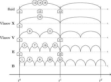
Start leap frog scheme with half a step of magnetic field (not repeated).

Calculate initial currents and send them to Maxwell solver (not repeated).

Distribute electromagnetic fields.

–

Advance electromagnetic fields to time $t_{0}+\frac{1}{2}\Delta t$ respectively half a substep further through subcycling.

–

Complete step of Vlasov solver.

Euler step of fluid solver, so that fluid quantities live at time $t_{1}$.

Set higher moments of fluid from phase space density that already lives at $t_{1}$.

Second Runge-Kutta substep of fluid solver.

The higher moments at time $t_{0}+\frac{1}{2}\Delta t$ are gained through interpolation. The electromagnetic fields live at the correct time and are directly copied.

Last Runge-Kutta substep of fluid solver.

Correct phase space density on basis of fluid quantities.

Calculate currents at $t_{1}$ and send them to Maxwell solver.

–

Advance electromagnetic fields to time $t_{1}$ respectively half a substep further. The value of B at time $t_{1}$ can be approximated through interpolation.

Figure 1: Stepping scheme for coupling of three-dimensional fluid-, Vlasov and Maxwell equations.

In the explicit schemes that are used here, each physical quantity always lives at a specific individual time, depending on how far the respective scheme has proceeded. During the simulation, these times may differ between the various quantities and the interstations may be different for each scheme. It is important that such times fit together when the respective schemes communicate with each other.If these time issues are not addressed, a variety of instabilities can occur, depending on the respective situation. In order to adapt them to each other the schemes are subdivided into atomic substeps, ie. smallest units of time stepping after that a stop leaves the data in a valid state with a well-defined time. These substeps are carried out in such an order that all the data has the appropriate time if communication has to take place. For that to be possible it may be necessary to adapt the numerical schemes slightly, for example by choosing a suitable Runge-Kutta method or artificially subdividing parts of the update procedure for obtaining intermediate results. In some cases, interpolation may be necessary for getting appropriate data.

The time layout of the coupling between the three-dimensional Vlasov solver, fluid models and Maxwell’s equations is shown and described in 1. Because the time scale given by the speed of light normally exceeds other time scales in the simulation by far, sub-cycling for the electromagnetic may be used to some degree in order to avoid unnecessarily many expensive Vlasov steps.

5 Benchmarks

In order to test the correction scheme, several benchmark problems are considered. First, a preliminary examination of the basic idea is conducted: Different two-dimensional distributions are rotated with constant angular velocity by means of the advection scheme of the Vlasov solver described above. In a discretized simulation like that, the gyration leads to a purely artificial smearing of the distribution. The mellowing of this smearing by means of correction fitting is examined quantitatively. After this preliminary investigation, full simulations of a fast magnetosonic wave with and without correction fitting are considered as an example of a linear phenomenon with anisotropic pressure. The final benchmark for assessing correction fitting in a fully non-linear regime is a simulation of the GEM challenge with different numerical models, with and without correction fitting.

5.1 Fundamental test

As a first test case, the evolution of a Maxwellian-shaped, slightly decentered bulb with an initially rotational velocity distribution is observed in two-dimensional $(v_{x},v_{y})$-space.

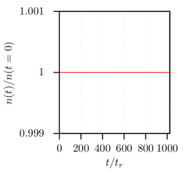
(a) density

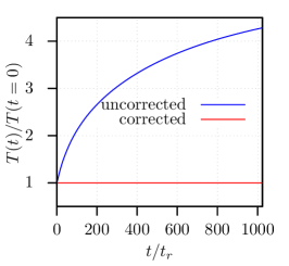
(b) temperature

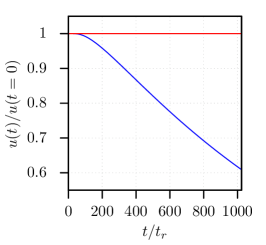
(c) velocity

Figure 2: Growth of temperature $T$ and velocity $u$ over time $t$ in the fundamental test with a slightly decentered Maxwellian-like distribution in velocity space. The normalized density (a), temperature (b) and absolute velocity (c) are depicted for the uncorrected and corrected case. Time is normalized to the time for one rotation, $t_{r}$.

In figure 2, the scalar temperature $T\sim\mathcal{E}-mn\textbf{u}^{2}/2$ (cf. (7)) and absolute velocity $u=|\textbf{u}|$ (cf. (5b)) are plotted against time for the uncorrected and corrected case, where the correction is enforced every step on $T$ and $u$. As expected, both observables stay on a constant level.

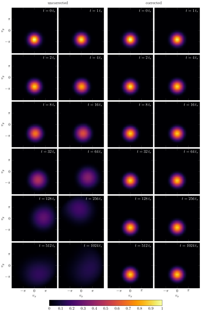
Figure 3: Evolution of the phase-space density over time in the fundamental test with a slightly decentered Maxwellian-like distribution in velocity space. The correction is done stepwise on velocity and temperature. Time is normalized to the time for one rotation, $t_{r}$.

In figure 3, the progression of the distribution is depicted. Its initial peak value is normalized to one. The uncorrected distribution apparently diffuses with time, but it stays constant in the corrected case.

As a second test case, the evolution of a completely non-Maxwellian, pacman-shaped, rotating, but slightly decentered velocity distribution is observed in two-dimensional $(v_{x},v_{y})$-space.

(a) density

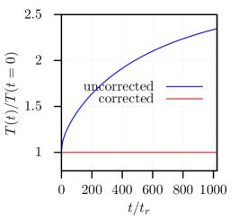
(b) temperature

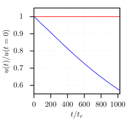
(c) velocity

Figure 4: Growth of temperature $T$ and velocity $u$ over time $t$ in the fundamental test with a slightly decentered pacman-like distribution in velocity space. The normalized density (a), temperature (b) and absolute velocity (c) are depicted for the uncorrected and corrected case. Time is normalized to the time for one rotation, $t_{r}$.

In figure 4, the scalar temperature $T$ and absolute velocity $u$ are again plotted against time for the uncorrected and corrected case. Still, both observables stay on a constant level.

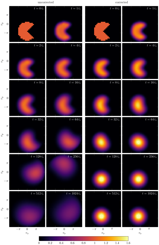
Figure 5: Evolution of the phase-space density over time in the fundamental test with a slightly decentered pacman-like distribution in velocity space. The correction is done stepwise on velocity and temperature. Time is normalized to the time for one rotation, $t_{r}$.

In figure 5, the progression of the distribution is depicted with its initial value normalized to one. The rotation is clockwise. Thus, in the uncorrected case, the rotation is a bit slower than expected from the initial values. The pacman diffuses with time and becomes Maxwellian-like, but its density basically stays the same in the corrected case.

5.2 Fast magnetosonic wave

The fast magnetosonic wave is a compressible wave with anisotropic pressure that propagates perpendicular to the magnetic field and occurs in the MHD regime. It has a phase velocity of

$$c_{\mathrm{fm}}^{2}=v_{\mathrm{A}}^{2}+\frac{3k_{\mathrm{B}}(T_{0,e}+T_{0,i})}{m_{i}}$$ (31)

where $v_{\mathrm{A}}$ is the Alfvén velocity. The initial conditions are

$$n_{s} =n_{0}\left(1+\frac{\delta v}{c_{\mathrm{fm}}}\cos(\omega t-kx)\right)$$ (32a)

$$\textbf{u}_{s} =\delta v\cos(\omega t-kx)\,\hat{\textbf{x}}$$ (32b)

J $$=\textbf{0}$$ (32c)

B $$=B_{0}\left(1+\frac{\delta v}{c_{\mathrm{fm}}}\cos(\omega t-kx)\right)\hat{\textbf{y}}$$ (32d)

E $$=-B_{0}\delta v\cos(\omega t-kx)\,\hat{\textbf{z}}$$ (32e)

$$p_{xx,s} =p_{0,s}\left(1+3\frac{\delta v}{c_{\mathrm{fm}}}\cos(\omega t-kx)\right)$$ (32f)

$$p_{yy,s}=p_{zz,s} =p_{0,s}\left(1+\frac{\delta v}{c_{\mathrm{fm}}}\cos(\omega t-kx)\right)$$ (32g)

The correction of the phase space density by means of ten-moment fitting is discussed on the basis of three simulations with similar parameters. One simulation is done with the pure Vlasov model, one with a pure ten-moment model and the last one with the Vlasov model in combination with the ten-moment model for correction. All parameters are consistent over the different simulations; the only differences are due to the fact that some of the parameters do not have a meaning in each of the configurations.

The simulation spans one transit of the wave through a periodic box with a size of 22.4 ion inertial lengths times 11.2 ion inertial lengths. In order to test the full two-dimensional code with this essentially one-dimensional wave, the direction of propagation is not parallel to the coordinate axes but skewed by an angle of $\operatorname{tan}^{-1}(2)$. With a wave length of ten ion inertial lengths and a phase velocity of twice the Alfvén velocity, the overall setup is thus still periodic, but in a non-trivial way. The speed of light is chosen to be $30\,v_{\mathrm{A}}$, the mass ratio is $m_{i}/m_{e}=25$, and the ion temperature is equal to the electron temperature. In the pure ten moment run, the value for $k_{0}$ is five inverse ion inertial lengths. The velocity spaces of ions and electrons are cubes with and edge length of ten ion inertial lengths and 20 ion inertial lengths, respectively. The spatial resolution is $64\times 32$ cells, while there are $32^{3}$ cells in each velocity space. The parameter $\varepsilon$ from the CWENO scheme is set to 0.1.

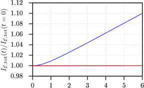
(a) total energy

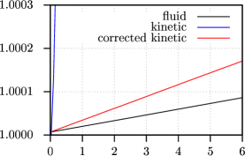
(b) total energy (details)

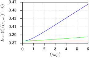
(c) partition among species

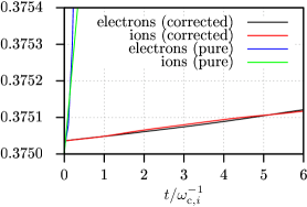
(d) partition (details)

Figure 6: Growth of energy over time in simulations of the fast magnetosonic wave with different models. The normalized total energy of the overall configuration is depicted in (a) and (b) for the three runs discussed in this section. In (c) and (d) the percental partition of thermal energy among electrons and ions is plotted for the pure kinetic run and the corrected kinetic run.

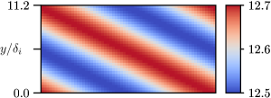
(a) $\mathbbm{E}_{xx,e}/{[\mathcal{E}]}$ (kinetic)

-

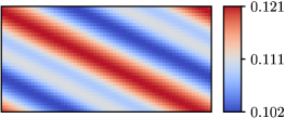
(b) $\mathbbm{E}_{xy,e}/{[\mathcal{E}]}$ (kinetic)

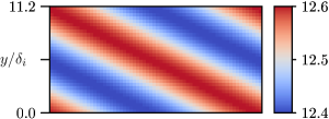
(c) $\mathbbm{E}_{xx,e}/{[\mathcal{E}]}$ (kinetic, corrected)

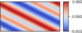
(d) $\mathbbm{E}_{xy,e}/{[\mathcal{E}]}$ (kinetic, corrected)

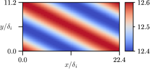
(e) $\mathbbm{E}_{xx,e}/{[\mathcal{E}]}$ (fluid)

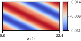
(f) $\mathbbm{E}_{xy,e}/{[\mathcal{E}]}$ (fluid)

Figure 7: Selected components of the electron energy tensor $\mathbbm{E}_{e}$ after one wave-transit in simulations of the fast magnetosonic wave with different models.

As it can be seen in (6), the numerical heating actually is an issue in the pure kinetic simulation. The integral of the total energy $I_{\mathcal{E},\mathrm{tot}}$ rises by about 10% over the course of the simulation. In 6(c), where the analogously defined thermal part $I_{\mathcal{E},\mathrm{th}}$ of $I_{\mathcal{E},\mathrm{tot}}$ and its distribution among the species in the plasma is plotted, it becomes apparent that by far the largest part of the energy growth is due to an increase in the inner energy of the electrons. This and the fact that the rise is almost linear is an indication that the heating is a consequence of the gyro motion and the concomitant smearing of the distribution function, just as it could be expected. The lighter electrons gyrate faster and are thus more susceptible for this effect.

The correction with ten-moment fitting leads to energy conservation that is almost as good as that of the pure fluid simulation. It must be kept in mind that for reasons of efficiency on the graphics cards only single precision floating point numbers are used, so that a better result can hardly be expected. Interestingly, there is practically no difference with respect to energy conservation between electrons and ions, when fitting is used (6(d)). The mass ration seems to play no role in that case.

A view on the actual results of the simulations (7) reveals noticeable differences between the simulations in the more critical quantities like the off-diagonal components of the energy tensor. The corrected kinetic run appears to lie in between the pure kinetic and the pure fluid run, but from the few low-resolution runs that were made it is hard to judge which of the runs is closer to the right result. In any way, it cannot be expected that the kinetic model leads to the same results as the ten-moment model that is artificially closed at the level of the heat flux and relies on additional parameters. Besides that, a small amplitude wave is probably not the best candidate for identifying actual problems with the behavior of the different schemes. The other results below are better suited for this kind of analysis.

In summary, the correction with ten-moment fitting leads to remarkably good conservation properties and at least seems to not introduce obviously wrong side-effects.

5.3 GEM challenge

The GEM challenge [27] is a well-studied problem for examining magnetic reconnection. The initial setup is a Harris sheet [28] that is periodic in the $x$-direction:

E $$=\textbf{0}$$ (33a)

B $$=B_{0}\tanh\left(\frac{y}{\lambda}\right)\hat{\textbf{x}}$$ (33b)

$$n_{s} =n_{\mathrm{bg}}+n_{0}\operatorname{sech}^{2}\left(\frac{y}{\lambda}\right)$$ (33c)

$$\textbf{u}_{s} =-\frac{\Theta_{s}B_{0}}{q_{s}\mu_{0}\lambda n_{0}}\left(\frac{1}{1+\frac{n_{\mathrm{bg}}}{n_{0}}\cosh^{2}\left(\frac{y}{\lambda}\right)}\right)\hat{\textbf{z}}=\frac{\delta_{i}}{\lambda}\left(\frac{-\operatorname{sgn}(q_{s})\Theta_{s}}{1+\frac{n_{\mathrm{bg}}}{n_{0}}\cosh^{2}\left(\frac{y}{\lambda}\right)}\right)v_{\mathrm{A}}\hat{\textbf{z}}$$ (33d)

$$k_{\mathrm{B}}T_{yy,s} =\frac{\Theta_{s}B_{0}^{2}}{2\mu_{0}n_{0}}=\frac{1}{2}\Theta_{s}m_{i}v_{\mathrm{A}}^{2}$$ (33e)

This sheet is edged with conducting walls above and below. Reconnection is triggered with a magnetic island perturbation of the form:

$$\delta\textbf{B}=\hat{\textbf{z}}\times\nabla\left(\delta\psi\cos\left(\frac{2\pi x}{L_{x}}\right)\cos\left(\frac{\pi y}{L_{y}}\right)\right)=\delta\psi\begin{pmatrix}-\frac{\pi}{L_{y}}\cos\left(\frac{2\pi x}{L_{x}}\right)\sin\left(\frac{\pi y}{L_{y}}\right)\\ \phantom{-}\frac{2\pi}{L_{x}}\sin\left(\frac{2\pi x}{L_{x}}\right)\cos\left(\frac{\pi y}{L_{y}}\right)\\ 0\end{pmatrix}$$ (34)

A variety of simulations of the GEM challenge are done. While the physical and most of the numerical parameters are kept constant as far as possible, the models, some methods, and certain numerical parameters are varied. The runs with the distinguishing parameters and names for later reference are listed in tables (1, 2). They differ with respect to the combination of physical models, the way in which the fitting matrix A is calculated, and the parameter $\varepsilon$, which determines the amount of numerical diffusivity in the CWENO scheme referenced above in 3.2. A larger $\varepsilon$ corresponds to less artificial diffusivity.

In all simulations, the physical parameters are the same: The domain has a size of $8\pi\times 4\pi$ ion intertial lengths, the ratio between the speed of light and the Alfvén velocity is 20 and the amplitude of the initial magnetic perturbation is $0.1\,B_{0}$. Furthermore, $m_{i}/m_{e}=25$ and $T_{i}/T_{e}=5$. In the Vlasov simulations, the velocity spaces are cubes with an edge length of 24 ion inertial lengths for electrons and 10 ion inertial lenghts for ions. In the pure ten-moment runs, the parameter $k_{0}$ introduced in (12) is set to five inverse ion inertial lengths, following Wang et al. [13]. All runs are done with a resolution of $256\times 128$ cells in physical space. If relevant, the velocity space is resolved with $32^{3}$ cells at each point in space.

name	model	$\varepsilon$	calculation of A
GEM-5-S	pure five-moment fluid	$1\text{\times}{10}^{-6}$	–
GEM-5-M	pure five-moment fluid	0.1	–
GEM-10-S	pure ten-moment fluid	$1\text{\times}{10}^{-6}$	–
GEM-10-M	pure ten-moment fluid	0.1	–
GEM-V	pure Vlasov model	–	–
GEM-V5-S	Vlasov + five-moment fluid	$1\text{\times}{10}^{-6}$	–
GEM-V5-M	Vlasov + five-moment fluid	0.1	–
GEM-V10-SG	Vlasov + ten-moment fluid	$1\text{\times}{10}^{-6}$	gradient descent
GEM-V10-MG	Vlasov + ten-moment fluid	0.1	gradient descent
GEM-V10-SA	Vlasov + ten-moment fluid	$1\text{\times}{10}^{-6}$	approximate
GEM-V10-MA	Vlasov + ten-moment fluid	0.1	approximate

Table 1: Parameters for the simulations of the GEM challenge. The omissions indicate that the respective category has no counterpart in the respective setup; for example, there is no fitting matrix in a pure fluid run.

The different simulations of the GEM challenge can be compared in a huge variety of ways. Here, some of these that are particularly illustrative in one way or another are picked out in order to give a clear picture.

As often in reconnection and for making the comparison with the data from the literature possible, the first thing to look at is the reconnected magnetic flux over time. For the current configuration, this flux can be measured as the integral of $|B_{y}|$ along the current sheet. Plots of this quantity over time are given in 8 for all simulations. While the growth rates all indicate fast reconnection and lie around a value of $0.2\,B_{0}v_{\mathrm{A}}$, which is comparable to the results presented by Birn et al. [27], the beginning of the process is at very different times and (at least) two groups of runs can clearly be distinguished: The flux in the simulations of the first group, the pure kinetic simulation and the kinetic simulations with ten-moment fitting, saturates at a value of around $3\,B_{0}\delta_{i}$ and at a time between 25 and 30 inverse ion gyro periods, which is very similar to what is shown for hybrid and particle runs in [27]. The second group consists of all other runs. The reconnected flux in these simulations does not saturate over the given period of time and resembles the Hall MHD curve in [27], which might partly be due to the low resolution that may suppress some two-fluid effects. The Vlasov runs with five-moment fitting have different curves than the simulations of the first groups and exhibit signs of artificial oscillations. They could not even be completed due to onsetting numerical instabilities.

There are at least three important results from this first comparison: Firstly, the ten-moment fitting correction delays the commencement of reconnection and leads to saturation at a slightly lower level, but the shape of the resulting curve is very similar to the kinetic one. With the pure ten-moment model, the onset of reconnection is significantly later. Secondly, all methods of ten-moment fitting that are tested lead to basically the same curve, which is remarkable, when compared to the variation between the two pure ten-moment runs that only differ with respect to the numerical parameter $\varepsilon$. Such differences seem to play a minor role when fitting is employed. Thirdly, five-moment correction fitting might work for simple test cases, but for general problems with non-linear dynamics isotropic fitting appears to influence the simulation heavily and render it invalid.

The main purpose of correction fitting is to get better conservation properties and in particular less artificial heating in the Vlasov code. This can be checked by examining the integral of the total energy $\mathcal{E}_{\mathrm{tot}}$ over the whole domain that is plotted depending on the time and for the different runs in 9. Here, the shortcomings of five-moment fitting become even more apparent than in 8. Non-physical oscillations are present almost from the beginning and the curves from the five-moment fitting runs do not resemble the results from the more plausible simulations in any way. Besides that, independently of the way in which ten-moment fitting is done, energy conservation is significantly improved through the correction routines. While the overall energy rises by about 27% in the pure kinetic simulation, the overall increase in energy hardly exceeds 1% for all other runs. This is not as good as the almost perfect conservation in the fluid codes or the results from the fast magnetosonic wave, but it must be taken into account that by far the majority of the energy increase stems from the phase around the time of the peak reconnection rate, when the conditions are more extreme, because all quantities vary faster and $f_{s}$ exhibits a higher anisotropy. Contrary to the poor discriminability of the curves of the ten-moment fitting runs in 8, both $\varepsilon$ and the method for calculating A make a difference with respect to energy conservation. A smaller $\varepsilon$ and an approximate calculation of A appear to lead to better energy conservation. The last point is not very unambiguous for the small $\varepsilon$, but it might be explained with the more noisy values of A that happen to be the result of the gradient descent method.

The reconnection curves and the energy curves are good for an overview, but they hide the details of the mechanisms with which they were generated. In order to get a better picture of qualitative differences between the runs, the structure of the current sheet, ie. the value of $J_{z}$, is given for times of comparable reconnected flux in 10. Here, the differences between the runs become more apparent: GEM-V10-MA exhibits a very similar structure to that in GEM-V. In both of them, the current sheet is split apart and $J_{z}$ is concentrated in two channels at the end points of the respective gap. Nevertheless, the velocities in $z$-direction and in particular $v_{z,e}$ are still peaked around the X-point. The two pure fluid runs that are shown are very different; they developed a clearer global X-point structure with a distinct sheet at the reconnection site. The most interesting observation is that GEM-V5-M is closer to the fluid runs than to the pure kinetic ones, whereby it does not fall clearly into one of the two categories and exhibits features that cannot be found in the other plots.

So, while five-moment fitting introduces all kinds of side-effects, ten-moment fitting appears to do what it is expected to: it improves energy conservation while retaining the kinetic mechanisms. For a further check of this, consider the electron phase space density near the X-point at the time of peak reconnection rate 11. There is a clear qualitative similarity between the shapes of the isosurfaces, but they are far from being equal. The two surfaces might be described as distorted versions of each other. At this level it is hard to say which of the two is more correct; other metrics like the conservation properties discussed above are probably better for judging the overall quality of the schemes. Anyway the results from the fitting run do not appear to be implausible in comparison to that of the pure kinetic run and on a qualitative level they are basically the same.

In summary it can be said that ten-moment fitting significantly improves the conservation properties of the Vlasov code without introducing spurious extra-effects. Approximate calculation of the fitting matrix A seems to be the better idea and a smaller $\varepsilon$ in the CWENO scheme leads to a lower increase in total energy, but in particular the last point is not very strict and the actual differences between the tested methods of ten-moment fitting are remarkably small, both in the data shown and in the other quantities that were not discussed in detail. On the other hand, five-moment fitting does not work well. Forcing the distribution function to match the moments of an essentially isotropic fluid model apparently destroys essential kinetic features, leads to artificial instabilities and renders the overall simulation useless.

name	resolution	$n_{v}$	$L_{v,e}/v_{\mathrm{A}}$	$L_{v,i}/v_{\mathrm{A}}$	$\varepsilon$	$\delta_{i}k_{0}$	calculation of A
GEM-5-S	$256\times 128$	–	–	–	$1\text{\times}{10}^{-6}$	–	–
GEM-5-M	$256\times 128$	–	–	–	0.1	–	–
GEM-10-S	$256\times 128$	–	–	–	$1\text{\times}{10}^{-6}$	5	–
GEM-10-M	$256\times 128$	–	–	–	0.1	5	–
GEM-V	$256\times 128$	32	24	10	–	–	–
GEM-V5-S	$256\times 128$	32	24	10	$1\text{\times}{10}^{-6}$	–	–
GEM-V5-M	$256\times 128$	32	24	10	0.1	–	–
GEM-V10-SG	$256\times 128$	32	24	10	$1\text{\times}{10}^{-6}$	–	gradient descent
GEM-V10-MG	$256\times 128$	32	24	10	0.1	–	gradient descent
GEM-V10-SA	$256\times 128$	32	24	10	$1\text{\times}{10}^{-6}$	–	approximate
GEM-V10-MA	$256\times 128$	32	24	10	0.1	–	approximate

Table 2: Parameters for the simulations of the GEM challenge. The omissions indicate that the respective category has no counterpart in the respective setup; for example, there is nothing like a resolution and size of a velocity in pure fluid simulations.

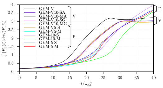
Figure 8: Reconnected flux over time in the different simulations of the GEM challenge.

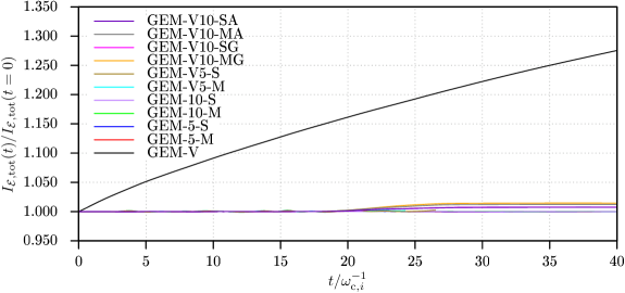
(a) Overview.

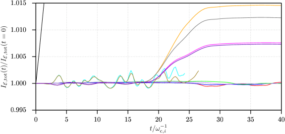
(b) Details.

Figure 9: Normalized total integrated energy over time in different simulations of the GEM challenge. For the exact definition of the total energy $I_{\mathcal{E},\mathrm{tot}}$ including the kinetic particle energy and the contributions from the electromagnetic fields. Because of the large differences between the ranges of the curves, two plots of the same data with different scaling are given.

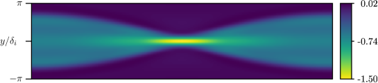
(a) GEM-10-M ($t=28.75\,\omega_{\mathrm{c},i}^{-1}$)

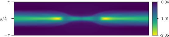
(b) GEM-V10-MA ($t=20.50\,\omega_{\mathrm{c},i}^{-1}$)

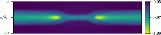
(c) GEM-V ($t=17.50\,\omega_{\mathrm{c},i}^{-1}$)

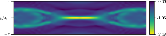
(d) GEM-V5-M ($t=24.25\,\omega_{\mathrm{c},i}^{-1}$)

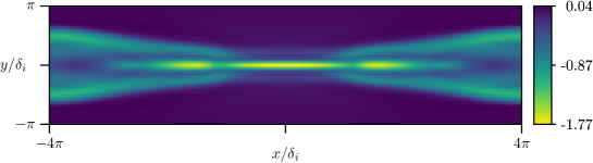
(e) GEM-5-M ($t=24.25\,\omega_{\mathrm{c},i}^{-1}$)

Figure 10: $J_{z}/(en_{0}v_{\mathrm{A}})$ in GEM challenge; comparison of different numerical schemes and models at time of comparable reconnected flux, roughly at time of highest reconnection rate (cf. 8).

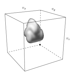
(a) GEM-V ($t=18.50\omega_{\mathrm{c},i}^{-1}$)

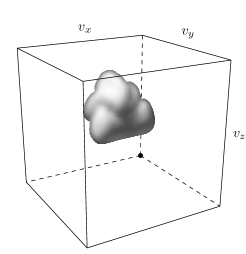
(b) GEM-V10-MG ($t=20.75\omega_{\mathrm{c},i}^{-1}$)

Figure 11: Isosurface of $f_{e}(\textbf{v})$ in different simulations of GEM challenge during time of peak reconnection rate in vicinity of X-point at $\textbf{x}=(x,y)\approx(0.15\delta_{i},-0.15\delta_{i})$.

6 Results and conclusion

A general method for enhancing the conservation properties of Vlasov solvers working on a spatial grid is proposed that is not bound to a specific numerical scheme. The method is tested on different test problems that stress several aspects like the behavior in the linear or the fully non-linear regime. It is found that the fully anisotropic correction scheme gives satisfactory results and very good conservation properties in all cases, while the related isotropic fitting procedure, of which the first is a generalization, leads to numerical instabilities and can thus not be used.

The next step is the application of the ten-moment fitting method to the problem of coupling fluid and kinetic codes that live in separate regions, as a generalization of the method presented in [1], also in combination with the correction method shown here. The respective results will be published in a future paper.

References

- Rieke et al. [2015] M. Rieke, T. Trost, R. Grauer, Coupled Vlasov and two-fluid codes on GPUs, Journal of Computational Physics 283 (2015) 436–452.
- Arnold and Giering [1997] A. Arnold, U. Giering, An analysis of the Marshak conditions for matching Boltzmann and Euler equations, Math. Models Methods Appl. Sci. 7 (1997) 557–577.
- Degond et al. [2010] P. Degond, G. Dimarce, L. Mieussens, A multiscale kinetic-fluid solver with dynamic localization of kinetic effects, J. Comput. Phys. 229 (2010) 4907–4933.
- Dellacherie [2003] S. Dellacherie, Kinetic-Fluid Coupling in the Field of the Atomic Vapor Isotopic Separation: Numerical Results in the Case of a Monospecies Perfect Gas, AIP Conf. Proc. 663 (2003) 947–956.
- Goudon et al. [2013] T. Goudon, S. Jin, J.-G. Liu, B. Yan, Asymptotic-preserving schemes for kinetic-fluid modeling of disperse two-phase flows., J. Comput. Phys. 246 (2013) 145–164.
- Klar et al. [2000] A. Klar, H. Neunzert, J. Struckmeier, Transition from Kinetic theory to macroscopic fluid equations: A problem for domain decompo sition and a source for new algorithms, Transport Theor. Stat. 29 (2000) 93–106.
- Tiwari and Klar [1998] S. Tiwari, A. Klar, An adaptive domain decomposition procedure for Boltzmann and Euler equations, J. Comput. Appl. Math. 90 (1998) 223–237.
- Tiwari et al. [2013] S. Tiwari, A. Klar, S. Hardt, A. Donkov, Coupled solution of the Boltzmann and Navier-Stokes equations in gas-liquid two phase flow, Comput. Fluids 71 (2013) 283–296.
- Le Tallec and Mallinger [1997] P. Le Tallec, F. Mallinger, Coupling Boltzmann and Navier-Stokes Equations by Half Fluxes, J. Comput. Phys. 136 (1997) 51–67.
- Sugiyama and Kusano [2007] T. Sugiyama, K. Kusano, Multi-scale plasma simulation by the interlocking of magnetohydrodynamic model and particle-in-cell kinetic model, J. Comput. Phys. 227 (2007) 1340–1352.
- Daldorff et al. [2014] L. K. S. Daldorff, G. Tóth, T. I. Gombosi, G. Lapenta, J. Amaya, S. Markidis, J. U. Brackbill, Two-way coupling of a global Hall magnetohydrodynamics model with a local implicit particle-in-cell model, J. Comput. Phys. 268 (2014) 236–254.
- Markidis et al. [2014] S. Markidis, P. Henri, G. Lapenta, K. Rönnmark, M. Hamrin, Z. Meliani, E. Laure, The Fluid-Kinetic Particle-in-Cell method for plasma simulations, J. Comput. Phys. (2014) 415–429.
- Wang et al. [2015] L. Wang, A. H. Hakim, A. Bhattacharjee, K. Germaschewski, Comparison of multi-fluid moment models with particle-in-cell simulations of collisionless magnetic reconnection, Physics of Plasmas 22 (2015) 012108.
- Johnson [2013] E. A. Johnson, Gaussian-moment relaxation closures for verifiable numerical simulation of fast magnetic reconnection in plasma, Ph.d. thesis, University of Wisconsin, Madison, 2013. Eprint arXiv:1409.6985 [physics.plasm-ph].
- Schmitz and Grauer [2006a] H. Schmitz, R. Grauer, Comparison of time splitting and backsubstitution methods for integrating Vlasov’s equation with magnetic fields, Comp. Phys. Commun. 175 (2006a) 86–92.
- Schmitz and Grauer [2006b] H. Schmitz, R. Grauer, Darwin–Vlasov simulations of magnetised plasmas, J. Comput. Phys. 214 (2006b) 738–756.
- Umeda and Fukazawa [2015] T. Umeda, K. Fukazawa, A high-resolution global Vlasov simulation of a small dielectric body with a weak intrinsic magnetic field on the K computer, Earth, Planets and Space 67 (2015) 49.
- Filbet et al. [2001] F. Filbet, E. Sonnendrücker, P. Bertrand, Conservative numerical schemes for the Vlasov equation, J. Comput. Phys. 172 (2001) 166–187.
- Kurganov and Levy [2000] A. Kurganov, D. Levy, A Third-Order Semidiscrete Central Scheme for Conservation Laws and Convection-Diffusion Equations, SIAM J. Sci. Comput. 22 (2000) 1461–1488.
- Shu and Osher [1988] C. W. Shu, S. Osher, Efficient Implementation of Essentially Non-oscillatory Shock-Capturing Schemes, J. Comput. Phys. 77 (1988) 439–471.
- Yee [1966] K. S. Yee, Numerical Solution of Initial Boundary Value Problems Involving Maxwell’s Equations in Isotropic Media, IEEE Trans. Antennas Propag. 14 (1966) 302–307.
- Taflove and Brodwin [1975] A. Taflove, M. E. Brodwin, Numerical Solution of Steady-State Electromagnetic Scattering Problems Using the Time-Dependent Maxwell’s Equations, IEEE Trans. Microwave Theory Tech. 23 (1975) 623–630.
- Tikhonov [1963] A. Tikhonov, Solution of incorrectly formulated problems and the regularization method, Soviet Mathematics Doklady 4 (1963) 1035–1038.
- Cauchy [1847] A. Cauchy, Méthode générale pour la résolution des systemes d’équations simultanées, Comptes Rendus de l’Académie des Sciences 25 (1847) 536–538.
- Press et al. [2007] W. H. Press, S. A. Teukolsky, W. T. Vetterling, B. P. Flannery, Numerical Recipes 3rd Edition: The Art of Scientific Computing, third ed., Cambridge University Press, New York, NY, USA, 2007.
- Leslie and Purser [1995] L. M. Leslie, R. J. Purser, Three-dimensional mass-conserving semi-Lagrangian scheme employing forward trajectories, Monthly Weather Review 123 (1995) 2551–2566.
- Birn et al. [2001] J. Birn, J. F. Drake, M. A. Shay, Geospace Environmental Modeling (GEM) Magnetic Reconnection Challenge, J. Geophys. Res. 106 (2001) 3715–3719.
- Harris [1962] E. G. Harris, On a plasma sheath separating regions of oppositely directed magnetic field, Il Nuovo Cimento 23 (1962) 115–121.