Communication-Optimal Distributed Clustering

Abstract

Clustering large datasets is a fundamental problem with a number of applications in machine learning. Data is often collected on different sites and clustering needs to be performed in a distributed manner with low communication. We would like the quality of the clustering in the distributed setting to match that in the centralized setting for which all the data resides on a single site. In this work, we study both graph and geometric clustering problems in two distributed models: (1) a point-to-point model, and (2) a model with a broadcast channel. We give protocols in both models which we show are nearly optimal by proving almost matching communication lower bounds. Our work highlights the surprising power of a broadcast channel for clustering problems; roughly speaking, to spectrally cluster $n$ points or $n$ vertices in a graph distributed across $s$ servers, for a worst-case partitioning the communication complexity in a point-to-point model is $n\cdot s$, while in the broadcast model it is $n+s$. A similar phenomenon holds for the geometric setting as well. We implement our algorithms and demonstrate this phenomenon on real life datasets, showing that our algorithms are also very efficient in practice.

1 Introduction

Clustering is a fundamental task in machine learning with widespread applications in data mining, computer vision, and social network analysis. Example applications of clustering include grouping similar webpages by search engines, finding users with common interests in a social network, and identifying different objects in a picture or video. For these applications, one can model the objects that need to be clustered as points in Euclidean space $\mathbb{R}^{d}$, where the similarities of two objects are represented by the Euclidean distance between the two points. Then the task of clustering is to choose $k$ points as centers, so that the total distance between all input points to their corresponding closest center is minimized. Depending on different distance objective functions, three typical problems have been studied: $k$-means, $k$-median, and $k$-center.

The other popular approach for clustering is to model the input data as vertices of a graph, and the similarity between two objects is represented by the weight of the edge connecting the corresponding vertices. For this scenario, one is asked to partition the vertices into clusters so that the “highly connected” vertices belong to the same cluster. A widely-used approach for graph clustering is spectral clustering, which embeds the vertices of a graph into the points in $\mathbb{R}^{k}$ through the bottom $k$ eigenvectors of the graph’s Laplacian matrix, and applies $k$-means on the embedded points.

Both the spectral clustering and the geometric clustering algorithms mentioned above have been widely used in practice, and have been the subject of extensive theoretical and experimental studies over the decades. However, these algorithms are designed for the centralized setting, and are not applicable in the setting of large-scale datasets that are maintained remotely by different sites. In particular, collecting the information from all the remote sites and performing a centralized clustering algorithm is infeasible due to high communication costs, and new distributed clustering algorithms with low communication cost need to be developed.

There are several natural communication models, and we focus on two of them: (1) a point-to-point model, and (2) a model with a broadcast channel. In the former, sometimes referred to as the message-passing model, there is a communication channel between each pair of users. This may be impractical, and the so-called coordinator model can often be used in place; in the coordinator model there is a centralized site called the coordinator, and all communication goes through the coordinator. This affects the total communication by a factor of two, since the coordinator can forward a message from one server to another and therefore simulate a point-to-point protocol. There is also an additional additive $O(\log s)$ bits per message, where $s$ is the number of sites, since a server must specify to the coordinator where to forward its message. In the model with a broadcast channel, sometimes referred to as the blackboard model, the coordinator has the power to send a single message which is received by all $s$ sites at once. This can be viewed as a model for single-hop wireless networks.

In both models we study the total number of bits communicated among all sites. Although the blackboard model is at least as powerful as the message-passing model, it is often unclear how to exploit its power to obtain better bounds for specific problems. Also, for a number of problems the communication complexity is the same in both models, such as computing the sum of $s$ length-$n$ bit vectors modulo two, where each site holds one bit vector [21], or estimating large moments [23]. Still, for other problems like set disjointness it can save a factor of $s$ in the communication [5].

1.1 Our contributions

We present algorithms for graph clustering: for any $n$-vertex graph whose edges are arbitrarily partitioned across $s$ sites, our algorithms have communication cost $\widetilde{O}(ns)$ in the message passing model, and have communication cost $\widetilde{O}(n+s)$ in the blackboard model, where the $\widetilde{O}$ notation suppresses polylogarithmic factors. The algorithm in the message passing model has each site send a spectral sparsifier of its local data to the coordinator, who then merges them in order to obtain a spectral sparsifier of the union of the datasets, which is sufficient for solving the graph clustering problem. Our algorithm in the blackboard model is technically more involved, as we show a particular recursive sampling procedure for building a spectral sparsifier can be efficiently implemented using a broadcast channel. It is unclear if other natural ways of building spectral sparsifiers can be implemented with low communication in the blackboard model. Our algorithms demonstrate the surprising power of the blackboard model for clustering problems. Since our algorithms compute spectral sparsifiers, they also have applications to solving symmetric diagonally dominant linear systems in a distributed model. Any such system can be converted into a system involving a Laplacian (see, e.g., [1]), from which a spectral sparsifier serves as a good preconditioner.

Next we show that $\Omega(ns)$ bits of communication is necessary in the message passing model to even recover a constant fraction of a cluster, and $\Omega(n+s)$ bits of communication is necessary in the blackboard model. This shows the optimality of our algorithms up to poly-logarithmic factors.

We then study clustering problems in constant-dimensional Euclidean space. We show for any $c>1$, computing a $c$-approximation for $k$-median, $k$-means, or $k$-center correctly with constant probability in the message passing model requires $\Omega(sk)$ bits of communication. We then strengthen this lower bound, and show even for bicriteria clustering algorithms, which may output a constant factor more clusters and a constant factor approximation, our $\Omega(sk)$ bit lower bound still holds. Our proofs are based on communication and information complexity. Our results imply that existing algorithms [3] for $k$-median and $k$-means with $\widetilde{O}(sk)$ bits of communication, as well as the folklore parallel guessing algorithm for $k$-center with $\widetilde{O}(sk)$ bits of communication, are optimal up to poly-logarithmic factors. For the blackboard model, we present an algorithm for $k$-median and $k$-means that achieves an $O(1)$-approximation using $\widetilde{O}(s+k)$ bits of communication. This again separates the models.

We give empirical results which show that using spectral sparsifiers preserves the quality of spectral clustering surprisingly well in real-world datasets. For example, when we partition a graph with over $70$ million edges (the Sculpture dataset) into $30$ sites, only $6\%$ of the input edges are communicated in the blackboard model and $8\%$ are communicated in the message passing model, while the values of the normalized cut (the objective function of spectral clustering) given in those two models are at most $2\%$ larger than the ones given by the centralized algorithm, and the visualized results are almost identical. This is strong evidence that spectral sparsifiers can be a powerful tool in practical, distributed computation. When the number of sites is large, the blackboard model incurs significantly less communication than the message passing model, e.g., in the Twomoons dataset when there are $90$ sites, the message passing model communicates $9$ times as many edges as communicated in the blackboard model, illustrating the strong separation between these models that our theory predicts.

1.2 Related work

There is a rich literature on spectral and geometric clustering algorithms from various aspects (see, e.g., [2, 19, 20, 22]). Balcan et al. [3, 4] and Feldman et al. [10] study distributed $k$-means ([3] also studies $k$-median), and present provable guarantees on the clustering quality. Very recently Guha et al. [11] studied distributed $k$-median/center/means with outliers. Cohen et al. [7] study dimensionality reduction techniques for the input data matrices that can be used for distributed $k$-means. The main takeaway is that there is no previous work which develops protocols for spectral clustering in the common message passing and blackboard models, and lower bounds are lacking as well. For geometric clustering, while upper bounds exist (e.g., [3, 4, 10]), no provable lower bounds in either model existed, and our main contribution is to show that previous algorithms are optimal. We also develop a new protocol in the blackboard model.

2 Preliminaries

Let $G=(V,E,w)$ be an undirected graph with $n$ vertices, $m$ edges, and weight function $V\times V\rightarrow\mathbb{R}_{\geq 0}$. The set of neighbors of a vertex $v$ is represented by $N(v)$, and its degree is $d_{v}=\sum_{u\sim v}w(u,v)$. The maximum degree of $G$ is defined to be $\Delta(G)=\max_{v}\{d_{v}\}$. For any set $S\subseteq V$, let $\mu(S)\triangleq\sum_{v\in S}d_{v}$. For any sets $S,T\subseteq V$, we define $w(S,T)\triangleq\sum_{u\in S,v\in T}w(u,v)$ to be the total weight of edges crossing $S$ and $T$. We define the conductance of any set $S$ by

$$\phi(S)=\frac{w(S,V\setminus S)}{\mu(S)}.$$

For two sets $X$ and $Y$, the symmetric difference of $X$ and $Y$ is defined as $X\triangle Y\triangleq(X\setminus Y)\cup(Y\setminus X)$.

For any matrix $A\in\mathbb{R}^{n\times n}$, let $\lambda_{1}(A)\leq\cdots\leq\lambda_{n}(A)=\lambda_{\max}(A)$ be the eigenvalues of $A$. For any two matrices $A,B\in\mathbb{R}^{n\times n}$, we write $A\preceq B$ to represent $B-A$ is positive semi-definite (PSD). Notice that this condition implies that $x^{\intercal}Ax\leq x^{\intercal}Bx$ for any $x\in\mathbb{R}^{n}$. Sometimes we also use a weaker notation $(1-\varepsilon)A\preceq_{r}B\preceq_{r}(1+\varepsilon)A$ to indicate that

$$(1-\varepsilon)x^{\intercal}Ax\leq x^{\intercal}Bx\leq(1+\varepsilon)x^{\intercal}Ax$$

for all $x$ in the row span of $A$.

2.1 Graph Laplacian

The Laplacian matrix of $G$ is an $n\times n$ matrix $L_{G}$ defined by $L_{G}=D_{G}-A_{G}$, where $A_{G}$ is the adjacency matrix of $G$ defined by $A_{G}(u,v)=w(u,v)$, and $D_{G}$ is the $n\times n$ diagonal matrix with $D_{G}(v,v)=d_{v}$ for any $v\in V[G]$. Alternatively, we can write $L_{G}$ with respect to a signed edge-vertex incidence matrix: we assign every edge $e=\{u,v\}$ an arbitrary orientation, and let $B_{G}(e,v)=1$ if $v$ is $e$’s head, $B_{G}(e,v)=-1$ if $v$ is $e$’s tail, and $B_{G}(e,v)=0$ otherwise. We further define a diagonal matrix $W_{G}\in\mathbb{R}^{m\times m}$, where $W_{G}(e,e)=w_{e}$ for any edge $e\in E[G]$. Then, we can write $L_{G}$ as $L_{G}=B_{G}^{\intercal}W_{G}B_{G}$. The normalized Laplacian matrix of $G$ is defined by $\mathcal{L}_{G}\triangleq D_{G}^{-1/2}L_{G}D_{G}^{-1/2}=I-D_{G}^{-1/2}A_{G}D_{G}^{-1/2}$. We sometimes drop the subscript $G$ when the underlying graph is clear from the context.

2.2 Spectral sparsification

For any undirected and weighted graph $G=(V,E,w)$, we say a subgraph $H$ of $G$ with proper reweighting of the edges is a $(1+\varepsilon)$-spectral sparsifier if

$$(1-\varepsilon)L_{G}\preceq L_{H}\preceq(1+\varepsilon)L_{G}.$$ (1)

By definition, it is easy to show that, if we decompose the edge set of a graph $G=(V,E)$ into $E_{1},\ldots,E_{\ell}$ for a constant $\ell$ and $H_{i}$ is a spectral sparsifier of $G_{i}=(V,E_{i})$ for any $1\leq i\leq\ell$, then the graph formed by the union of edge sets from $H_{i}$ is a spectral sparsifier of $G$. It is known that, for any undirected graph $G$ of $n$ vertices, there is a $(1+\varepsilon)$-spectral sparsifier of $G$ with $O(n/\varepsilon^{2})$ edges, and it can be constructed in almost-linear time [15].

The following lemma shows that a spectral sparsifier preserves the clustering structure of a graph.

Lemma 2.1.

Let $H$ be a $(1+\varepsilon)$-spectral sparsifier of $G$ for some $\varepsilon\leq 1/3$. Then, it holds for any set $S\subseteq V$ that $\phi_{H}(S)\in\left(\frac{1}{2},2\right)\phi_{G}(S)$.

Proof.

Let $x_{u}\in\mathbb{R}^{n}$ be the indicator vector of vertex $u$, i.e., $x_{u}(v)=1$ if $u=v$, and $x_{u}(v)=0$ otherwise. We have that

$$(1-\varepsilon)\cdot x_{u}^{\intercal}L_{G}x_{u}\leq x_{u}^{\intercal}L_{H}x_{u}\leq(1+\varepsilon)\cdot x_{u}^{\intercal}L_{G}x_{u},$$

which implies that $(1-\varepsilon)\cdot\mu_{G}(S)\leq\mu_{H}(S)\leq(1+\varepsilon)\cdot\mu_{G}(S)$ for any subset $S$.

Similarly, for any set $S\subseteq V$ we define the indicator vector of $S$ by $x_{S}\in\mathbb{R}^{n}$, where $x_{S}(u)=1$ if $u\in S$, and $x_{S}(u)=0$ otherwise. Hence, $x_{S}^{\intercal}L_{G}x_{S}=w_{G}(S,V\setminus S)$, and $x_{S}^{\intercal}L_{H}x_{S}=w_{H}(S,V\setminus S)$. Combining these with (1), we have that

$$(1-\varepsilon)\cdot w_{G}(S,V\setminus S)\leq w_{H}(S,V\setminus S)\leq(1+\varepsilon)\cdot w_{G}(S,V\setminus S).$$

Hence, for any subset $S$ we have that

$$\phi_{H}(S)=\frac{w_{H}(S,V\setminus S)}{\mu_{H}(S)}\leq\frac{(1+\varepsilon)w_{G}(S,V\setminus S)}{(1-\varepsilon)\mu_{G}(S)}\leq 2\cdot\phi_{G}(S),$$

where the last inequality holds by assuming $\varepsilon\leq 1/3$. Similarly, we have that

$$\phi_{H}(S)=\frac{w_{H}(S,V\setminus S)}{\mu_{H}(S)}\geq\frac{(1-\varepsilon)w_{G}(S,V\setminus S)}{(1+\varepsilon)\mu_{G}(S)}\geq\frac{1}{2}\cdot\phi_{G}(S).$$

Hence, $\phi_{H}(S)$ and $\phi_{G}(S)$ differ by at most a factor of 2 for any vertex set $S$. ∎

2.3 Models of computation

We study distributed clustering in two models for distributed data: the message passing model and the blackboard model. The message passing model represents those distributed computation systems with point-to-point communication, and the blackboard model represents those where messages can be broadcast to all parties.

More precisely, in the message passing model there are $s$ sites $\mathcal{P}_{1},\ldots,\mathcal{P}_{s}$, and one coordinator. These sites can talk to the coordinator through a two-way private channel. In fact, this is referred to as the coordinator model in Section 1, where it is shown to be equivalent to the point-to-point model up to small factors. The input is initially distributed at the $s$ sites. The computation is in terms of rounds: at the beginning of each round, the coordinator sends a message to some of the $s$ sites, and then each of those sites that have been contacted by the coordinator sends a message back to the coordinator. At the end, the coordinator outputs the answer. In the alternative blackboard model, the coordinator is simply a blackboard where these $s$ sites $\mathcal{P}_{1},\ldots,\mathcal{P}_{s}$ can share information; in other words, if one site sends a message to the coordinator/blackboard then all the other $s-1$ sites can see this information without further communication. The order for the sites to speak is decided by the contents of the blackboard.

For both models we measure the communication cost as the total number of bits sent through the channels. The two models are now standard in multiparty communication complexity (see, e.g., [5, 21, 23]). They are similar to the congested clique model [16] studied in the distributed computing community; the main difference is that in our models we do not post any bandwidth limitations at each channel but instead consider the total number of bits communicated.

2.4 Communication complexity

For any problem $\mathcal{A}$ and any protocol $\Pi$ solving $\mathcal{A}$, the communication complexity of a protocol $\Pi$ is the maximum communication cost of $\Pi$ over all possible inputs $X$. When the protocol is randomised, we define the error of $\Pi$ by

$$\max_{X}\mathbb{P}\left(\mbox{the coordinator outputs an incorrect answer on $X$}\right),$$

where the $\max$ is over all inputs $X$ and the probability is over all random strings of the coordinator and $s$ sites. The $\delta$-error randomised communication complexity $\mathsf{R}_{\delta}(\mathcal{A})$ of a problem $\mathcal{A}$ in the message passing model is the minimum communication complexity of any randomised protocol $\Pi$ that solves $\mathcal{A}$ with error at most $\delta$.

Let $\mu$ be an input distribution on $X$. We call a deterministic protocol $(\delta,\mu)\text{-error}$ if it gives the correct answer for $\mathcal{A}$ on at least a $1-\delta$ fraction of all input pairs, weighted by the distribution $\mu$. We denote $\mathsf{D}_{\delta,\mu}(\mathcal{A})$ as the cost of the minimum-communication $(\delta,\mu)\text{-error}$ protocol. A standard lemma in communication complexity called Yao’s minimax lemma shows that $\mathsf{R}_{\delta}(\mathcal{A})\geq\max_{\mu}\mathsf{D}_{\delta,\mu}(\mathcal{A}).$

2.5 Information complexity

We abuse notation by using $\Pi$ for both the protocol and its transcript (its concatenation of messages). In the message passing model, let $\Pi_{i}\ (i\in[s])$ be the transcript (set of messages exchanged) between the $i$-th site and the coordinator. Then $\Pi$ can be seen as a concatenation $\Pi_{1}\circ\Pi_{2}\circ\ldots\circ\Pi_{s}$ ordered by the timestamps of the messages. We define the information complexity of a problem $\mathcal{A}$ in the message passing model by

$$\mathsf{IC}_{\mu,\delta}(\mathcal{A})=\min_{(\delta,\mu)\text{-error}\ \Pi}\sum_{i\in[s]}I(X_{1},\ldots,X_{s};\Pi_{i}),$$

where $I(\cdot\ ;\ \cdot)$ is the mutual information function. It has been shown in [12] that $\mathsf{R}_{\delta}(\mathcal{A})\geq\mathsf{IC}_{\delta,\mu}(\mathcal{A})$ for any input distribution $\mu$.

3 Distributed graph clustering

In this section we study distributed graph clustering. We assume that the vertex set of the input graph $G=(V,E)$ can be partitioned into $k$ clusters, where vertices in each cluster $S$ are highly connected to each other, and there are fewer edges between $S$ and $V\setminus S$. To formalize this notion, we define the $k$-way expansion constant of graph $G$ by

$$\rho(k)\triangleq\min_{\mbox{\footnotesize partition $A_{1},\ldots,A_{k}$}}\max_{1\leq i\leq k}\phi_{G}(A_{i}).$$

Notice that a graph $G$ has $k$ clusters if the value of $\rho(k)$ is small. It was shown in [14] that $\rho(k)$ closely relates to $\lambda_{k}(\mathcal{L}_{G})$ by the following higher-order Cheeger inequality:

$$\frac{\lambda_{k}(\mathcal{L}_{G})}{2}\leq\rho(k)\leq O(k^{2})\sqrt{\lambda_{k}(\mathcal{L}_{G})}.$$

Hence, a large gap between $\lambda_{k+1}(\mathcal{L}_{G})$ and $\rho(k)$ implies (i) the existence of a $k$-way partition $\{S_{i}\}_{i=1}^{k}$ such that every $S_{i}$ has small conductance $\phi_{G}(S_{i})\leq\rho(k)$, and (ii) any $(k+1)$-way partition of $G$ contains a subset with high conductance $\rho(k+1)\geq\lambda_{k+1}(\mathcal{L}_{G})/2$. Therefore, a large gap between $\lambda_{k+1}(\mathcal{L}_{G})$ and $\rho(k)$ ensures that $G$ has exactly $k$ clusters. In the following, we assume that

$$\Upsilon\triangleq\lambda_{k+1}(\mathcal{L}_{G})/\rho(k)=\Omega(k^{3})$$

to ensure that the input graph $G$ has exactly $k$ clusters. The same assumption has been used in the literature for studying graph clustering in the centralized setting [20].

Both algorithms presented in the section are based on the following spectral clustering algorithm: (i) compute the $k$ eigenvectors $f_{1},\ldots,f_{k}$ of $\mathcal{L}_{G}$ associated with $\lambda_{1}(\mathcal{L}_{G}),\ldots,\lambda_{k}(\mathcal{L}_{G})$; (ii) embed every vertex $v$ to a point in $\mathbb{R}^{k}$ through the embedding

$$F(v)=\frac{1}{\sqrt{d_{v}}}\cdot(f_{1}(v),\ldots,f_{k}(v));$$

(iii) run $k$-means on the embedded points $\{F(v)\}_{v\in V}$, and group the vertices of $G$ into $k$ clusters according to the output of $k$-means.

3.1 The message passing model

We assume the edges of the input graph $G=(V,E)$ are arbitrarily allocated among $s$ sites $\mathcal{P}_{1},\cdots,\mathcal{P}_{s}$, and we use $E_{i}$ to denote the edge set maintained by site $\mathcal{P}_{i}$. Our proposed algorithm consists of two steps: (i) every $\mathcal{P}_{i}$ computes a linear-sized $(1+\varepsilon)$-spectral sparsifier $H_{i}$ of $G_{i}\triangleq(V,E_{i})$, for a small constant $\varepsilon\leq 1/10$, and sends the edge set of $H_{i}$, denoted by $E_{i}^{\prime}$, to the coordinator; (ii) the coordinator runs a spectral clustering algorithm on the union of received graphs $H\triangleq\left(V,\bigcup_{i=1}^{k}E_{i}^{\prime}\right)$. The theorem below summarizes the performance of this algorithm, and shows the approximation guarantee of this algorithm is as good as the provable guarantee of spectral clustering known in the centralized setting, which is shown in the lemma below.

Lemma 3.1 ([20]).

Let $G$ be a graph satisfying the condition $\Upsilon=\Omega(k^{3})$, and $k\in\mathbb{N}$. Then, a spectral clustering algorithm outputs sets $A_{1},\ldots,A_{k}$ such that $\mu(A_{i}\triangle S_{i})=O\left(k^{3}\cdot\Upsilon^{-1}\cdot\mu(S_{i})\right)$ holds for any $1\leq i\leq k$, where $S_{i}$ is the optimal cluster corresponding to $A_{i}$.

Theorem 3.2.

Let $G=(V,E)$ be an $n$-vertex graph with $\Upsilon=\Omega(k^{3})$, and suppose the edges of $G$ are arbitrarily allocated among $s$ sites. Assume $S_{1},\cdots,S_{k}$ is an optimal partition that achieves $\rho(k)$. Then, the algorithm above computes a partition $A_{1},\ldots,A_{k}$ satisfying $\mu(A_{i}\triangle S_{i})=O\left(k^{3}\cdot\Upsilon^{-1}\cdot\mu(S_{i})\right)$ for any $1\leq i\leq k$. The total communication cost of this algorithm is $\widetilde{O}(ns)$ bits.

Proof.

By the definition of the Laplacian matrix, we have that $L_{G}=\sum_{i=1}^{s}L_{G_{i}}$. Since every $H_{i}$ is a $(1+\varepsilon)$-spectral sparsifier of graph $G_{i}$, we have that $(1-\varepsilon)L_{H_{i}}\preceq L_{G_{i}}\preceq(1+\varepsilon)L_{H_{i}}$. This implies that $(1-\varepsilon)L_{H}\preceq L_{G}\preceq(1+\varepsilon)L_{H}$, by the definition of $H_{i}$ and graph Laplacians. Now we show that our assumption on $\Upsilon$ is preserved in $H$. By Lemma 2.1, we have for any $1\leq i\leq k$ that $\phi_{H}(S_{i})\in\left(\frac{1}{2},2\right)\phi_{G}(S_{i})$, which implies that $S_{i}$ has low conductance in $H$, and $\rho_{H}(k)\in\left(\frac{1}{2},2\right)\rho_{G}(k)$. To show that $\lambda_{k}(\mathcal{L}_{H})$ is a constant approximation of $\lambda_{k}(\mathcal{L}_{G})$, notice that

$$(1-c)\cdot x^{\intercal}L_{G}x\leq x^{\intercal}L_{H}x\leq(1+c)\cdot x^{\intercal}L_{G}x$$

holds for any $x\in\mathbb{R}^{n}$. Hence it holds for any $x\in\mathbb{R}^{n}$ that

$$(1-\varepsilon)\cdot x^{\intercal}D_{G}^{-1/2}L_{G}D_{G}^{-1/2}x\leq x^{\intercal}D_{G}^{-1/2}L_{H}D_{G}^{-1/2}x\leq(1+\varepsilon)\cdot x^{\intercal}D_{G}^{-1/2}L_{G}D_{G}^{-1/2}x.$$

Since $D_{G}^{-1/2}L_{G}D_{G}^{-1/2}=\mathcal{L}_{G}$ and $\frac{1}{2}D_{G}^{-1}\preceq D_{H}^{-1}\preceq 2D_{G}^{-1}$, we have that $\lambda_{i}\left(\mathcal{L}_{H}\right)=\Theta\left(\lambda_{i}\left(\mathcal{L}_{G}\right)\right)$, and the assumption on $\Upsilon$ in $H$ is preserved from $G$ up to a constant factor. By Lemma 3.1, the output of a spectral clustering algorithm on $H$ satisfies the claimed properties. The total communication cost of $\widetilde{O}(ns)$ bits follows from the fact that every $H_{i}$ has $O(n)$ edges. ∎

Next we show that the communication cost of our proposed algorithm is optimal up to a logarithmic factor. Our analysis is based on a reduction from graph clustering to the Multiparty Set-Disjointness problem ($\mathsf{DISJ}_{s,n}$): for any $s$ sites $\mathcal{P}_{1},\ldots,\mathcal{P}_{s}$, where each $\mathcal{P}_{i}$ has a set $S_{i}\subseteq[n]$, let $X_{i}=(X_{i}^{1},\ldots,X_{i}^{n})$ be the characteristic vector of $S_{i}$, and let $X=(X_{1},\ldots,X_{s})$ be the input matrix with $X_{i}$ being the $i$-th row. Let $X^{j}=(X_{1}^{j},\ldots,X_{s}^{j})$ be the $j$-th column of the input matrix $X$. We define a function $\mathsf{ALLONE}_{s}$ on an $s$-bit vector $Y=(Y_{1},\ldots,Y_{s})$ as $\text{{$\mathsf{ALLONE}_{s}$}}(Y)=\bigwedge_{i\in[s]}Y_{i}$, and $\text{{$\mathsf{DISJ}_{s,n}$}}(X)=\bigvee_{j\in[n]}\text{{$\mathsf{ALLONE}_{s}$}}(X^{j})$. Then the $\mathsf{DISJ}_{s,n}$ problem asks the value of $\text{{$\mathsf{DISJ}_{s,n}$}}(X)$. We introduce two hard input distributions for $\mathsf{ALLONE}_{s}$ and $\mathsf{DISJ}_{s,n}$ respectively.

• Hard input distribution $\nu$ on $Y\in\{0,1\}^{s}$ for $\mathsf{ALLONE}_{s}$: with probability $1/2$, we choose each $Y_{i}\ (i\in[s])$ to be $0$ or $1$ with equal probability; with probability $1/4$ we choose $Y$ to be an all-$1$ vector; and with the remaining probability $1/4$ we choose $Y$ to be a random vector with $n-1$ coordinates being $1$’s and a random coordinate being $0$.

• Hard input distribution $\mu_{n}$ on $X\in\{0,1\}^{s\times n}$ for $\mathsf{DISJ}_{s,n}$: For each $j\in[n]$, we choose $X^{j}\sim\nu$.

Theorem 3.3 ([5]).

It holds that $\mathsf{IC}_{0.49,\nu}(\text{{$\mathsf{ALLONE}_{s}$}})=\Omega(s)$, and $\mathsf{IC}_{0.49,\nu}(\text{{$\mathsf{DISJ}_{s,n}$}})=\Omega(sn)$.

Lemma 3.4.

In the message passing model, any randomized algorithm that computes $\mathsf{DISJ}_{s,n}$ correctly with probability $0.9$ needs $\Omega(sn)$ bits of communication.

Proof.

The lemma follows from Theorem 3.3 and Yao’s minimax lemma. ∎

Theorem 3.5.

Let $G$ be an undirected graph with $n$ vertices, and suppose the edges of $G$ are distributed among $s$ sites. Then, any algorithm that correctly outputs a constant fraction of a cluster in $G$ requires $\Omega(ns)$ bits of communication. This holds even if each cluster has constant expansion.

Proof.

Our proof is based on the reduction from graph clustering to the Multiparty Set-Disjointness problem ($\mathsf{DISJ}_{s,n}$). For any item $j$ and site $\mathcal{P}_{i}$, we set $X^{j}_{i}=0$ if item $j$ appears in site $\mathcal{P}_{i}$, and $X^{j}_{i}=1$ otherwise. Then $\text{{$\mathsf{DISJ}_{s,n}$}}(X)=1$ if there is some item not appearing in any site. Now we construct a graph $G$ based on the hard instance $X$ of $\mathsf{DISJ}_{n,s}$ as follows: initially, graph $G$ consists of $n$ isolated vertices $\ell_{1},\ldots,\ell_{n}$, and $r$ isolated vertices $r_{1},\ldots,r_{s}$. Then, we add an edge between $\ell_{j}$ and $r_{i}$ if item $j$ appears in site $\mathcal{P}_{i}$. With this construction, it is easy to see that $\text{{$\mathsf{DISJ}_{s,n}$}}(X)=0$ if every vertex $\ell_{j}$ is connected to some $r_{i}$, and $\text{{$\mathsf{DISJ}_{s,n}$}}(X)=1$ if there are some isolated vertices $\ell_{j}$.

We will show that, when $\text{{$\mathsf{DISJ}_{s,n}$}}(X)=0$, our constructed graph $G$ is a bipartite expander, i.e., $G$ has only $1$ cluster. To prove this, notice that, from the hard input distribution $\mu$ on $Y\in\{0,1\}^{s}$ described above, with probability $1/2$ we choose each $Y_{i}(i\in[s])$ to be $0$ or $1$ with equal probability. This implies that, for any $\ell_{i}$ and $r_{j}$, there is an edge between $\ell_{i}$ and $r_{j}$ independently with probability at least $1/4$. By standard results on constructing expanders, this implies $G$ is a bipartite expander with constant expansion, and in particular is connected.

On the other side, when $\text{{$\mathsf{DISJ}_{s,n}$}}(X)=1$, every isolated vertex $\ell_{j}$ itself forms a cluster with conductance $0$ and constant expansion, and the giant component of $G$ forms a cluster with conductance $0$ and constant expansion (since, as argued in the previous paragraph, it is a bipartite expander). Let $k$ be the number of connected components in graph $G$. Then, $\rho(k)=0$, and our assumption on $\Upsilon=\lambda_{k+1}(\mathcal{L}_{G})/\rho(k)=\Omega(k^{3})$ holds trivially. Hence any clustering algorithm that is able to find a constant fraction of each cluster in graph $G$ satisfying $\Upsilon=\Omega(k^{3})$ can be used to solve $\mathsf{DISJ}_{s,n}$. The lower bound on the communication complexity of graph clustering follows from the lower bound for $\mathsf{DISJ}_{s,n}$. ∎

As a remark, it is easy to see that this lower bound also holds for constructing spectral sparsifiers: for any $n\times n$ $\mathsf{PSD}$ matrix $A$ whose entries are arbitrarily distributed among $s$ sites, any distributed algorithm that constructs a $(1+\Theta(1))$-spectral sparsifier of $A$ requires $\Omega(ns)$ bits of communication. This follows since such a spectral sparsifier can be used to solve the spectral clustering problem. Spectral sparsification has played an important role in designing fast algorithms from different areas, e.g., machine learning, and numerical linear algebra. Hence our lower bound result for constructing spectral sparsifiers may have applications to studying other distributed learning algorithms.

3.2 The blackboard model

Next we present a graph clustering algorithm with $\widetilde{O}(n+s)$ bits of communication cost in the blackboard model. Our result is based on the observation that a spectral sparsifier preserves the structure of clusters, which was used for proving Theorem 3.2. So it suffices to design a distributed algorithm for constructing a spectral sparsifier in the blackboard model.

Our distributed algorithm is based on constructing a chain of coarse sparsifiers [18], which is described as follows: for any input PSD matrix $K$ with $\lambda_{\max}(K)\leq\lambda_{u}$ and all the non-zero eigenvalues of $K$ at least $\lambda_{\ell}$, we define $d=\lceil\log_{2}(\lambda_{u}/\lambda_{\ell})\rceil$ and construct a chain of $d+1$ matrices

$$[K(0),K(1),\ldots,K(d)],$$ (2)

where $\gamma(i)=\lambda_{u}/2^{i}$ and $K(i)=K+\gamma(i)I$. Notice that in the chain above every $K(i-1)$ is obtained by adding weights to the diagonal entries of $K(i)$, and $K(i-1)$ approximates $K(i)$ as long as the weights added to the diagonal entries are small. We will construct this chain recursively, so that $K(0)$ has heavy diagonal entries and can be approximated by a diagonal matrix. Moreover, since $K$ is the Laplacian matrix of a graph $G$, it is easy to see that $d=O(\log n)$ as long as the edge weights of $G$ are polynomially upper-bounded in $n$.

Lemma 3.6 ([18]).

The chain (2) satisfies the following relations: (1) $K\preceq_{r}K(d)\preceq_{r}2K$; (2) $K(\ell)\preceq K(\ell-1)\preceq 2K(\ell)$ for all $\ell\in\{1,\ldots,d\}$; (3) $K(0)\preceq 2\gamma(0)I\preceq 2K(0)$.

Based on Lemma 3.6, we will construct a chain of matrices

$$\left[\widetilde{K}(0),\widetilde{K}(1),\ldots,\widetilde{K}(d)\right]$$ (3)

in the blackboard model, such that every $\widetilde{K}(\ell)$ is a spectral sparsifier of $K(\ell)$, and every $\widetilde{K}(\ell+1)$ can be constructed from $\widetilde{K}(\ell)$. The basic idea behind our construction is to use the relations among different $K(\ell)$ shown in Lemma 3.6 and the fact that, for any $K=B^{\intercal}B$, sampling rows of $B$ with respect to their leverage scores can be used to obtain a matrix approximating $K$.

Theorem 3.7.

Let $G$ be an undirected graph on $n$ vertices, where the edges of $G$ are allocated among $s$ sites, and the edge weights are polynomially upper bounded in $n$. Then, a spectral sparsifier of $G$ can be constructed with $\widetilde{O}(n+s)$ bits of communication in the blackboard model. That is, the chain (3) can be constructed with $\widetilde{O}(n+s)$ bits of communication in the blackboard model.

Proof.

Let $K=B^{\intercal}B$ be the Laplacian matrix of the underlying graph $G$, where $B\in\mathbb{R}^{m\times n}$ is the edge-vertex incidence matrix of $G$. We will prove that every $\widetilde{K}(i+1)$ can be constructed based on $\widetilde{K}(i)$ with $\widetilde{O}(n+s)$ bits of communication. This implies that $\widetilde{K}(d)$, a $(1+\varepsilon)$-spectral sparsifier of $K$, can be constructed with $\widetilde{O}(n+s)$ bits of communication, as the length of the chain $d=O(\log n)$.

First of all, notice that $\lambda_{u}\leq 2n$, and the value of $n$ can be obtained with communication cost $\widetilde{O}(n+s)$ (different sites sequentially write the new IDs of the vertices on the blackboard). In the following we assume that $\lambda_{u}$ is the upper bound of $\lambda_{\max}$ that we actually obtained in the blackboard.

Base case of $\ell=0$: By definition, $K(0)=K+\lambda_{u}\cdot I$, and $\frac{1}{2}\cdot K(0)\preceq\gamma(0)\cdot I\preceq K(0)$, due to Statement 3 of Lemma 3.6. Let $\oplus$ denote appending the rows of one matrix to another. We define $B_{\gamma(0)}=B\oplus\sqrt{\gamma(0)}\cdot I$, and write $K(0)=K+\gamma(0)\cdot I=B^{\intercal}_{\gamma(0)}B_{\gamma(0)}$. By defining $\tau_{i}=b_{i}^{\intercal}\left(K(0)\right)^{\intercal}b_{i}$ for each row of $B_{\gamma(0)}$, we have $\tau_{i}\leq b_{i}^{\intercal}\left(\gamma(0)\cdot I\right)b_{i}\leq 2\cdot\tau_{i}$. Let $\widetilde{\tau}_{i}=b_{i}^{\intercal}\left(\gamma(0)\cdot I\right)^{+}b_{i}$ be the leverage score of $b_{i}$ approximated using $\gamma(0)\cdot I$, and let $\widetilde{\tau}$ be the vector of approximate leverage scores, with the leverage scores of the $n$ rows corresponding to $\sqrt{\gamma(0)}\cdot I$ rounded up to 1. Then, with high probability sampling $O(\varepsilon^{-2}n\log n)$ rows of $B$ will give a matrix $\widetilde{K}(0)$ such that $(1-\varepsilon)K(0)\preceq\widetilde{K}(0)\preceq(1+\varepsilon)K(0)$. Notice that, as every row of $B$ corresponds to an edge of $G$, the approximate leverage scores $\widetilde{\tau}_{i}$ for different edges can be computed locally by different sites maintaining the edges, and the sites only need to send the information of the sampled edges to the blackboard, hence the communication cost is $\widetilde{O}(n+s)$ bits.

Induction step: We assume that $(1-\varepsilon)K(\ell)\preceq_{r}\widetilde{K}(\ell)\preceq_{r}(1+\varepsilon)K(\ell)$, and the blackboard maintains the matrix $\widetilde{K}(\ell)$. This implies that $(1-\varepsilon)/(1+\varepsilon)\cdot K(\ell)\preceq_{r}1/(1+\varepsilon)\cdot\widetilde{K}(\ell)\preceq_{r}K(\ell).$ Combining this with Statement 2 of Lemma 3.6, we have that

$$\frac{1-\varepsilon}{2(1+\varepsilon)}K(\ell+1)\preceq_{r}\frac{1}{2(1+\varepsilon)}\widetilde{K}(\ell)\preceq K(\ell+1).$$

We apply the same sampling procedure as in the base case, and obtain a matrix $\widetilde{K}(\ell+1)$ such that $(1-\varepsilon)K(\ell+1)\preceq_{r}\widetilde{K}(\ell+1)\preceq_{r}(1+\varepsilon)K(\ell+1)$. Notice that, since $\widetilde{K}(\ell)$ is written on the blackboard, the probabilities used for sampling individual edges can be computed locally by different sites, and in each round only the sampled edges will be sent to the blackboard in order for the blackboard to obtain $\widetilde{K}(\ell+1)$. Hence, the total communication cost in each iteration is $\widetilde{O}(n+s)$ bits. Combining this with the fact that the chain length $d=O(\log n)$ proves the theorem. ∎

Combining Theorem 3.7 and the fact that a spectral sparsifier preserves the structure of clusters, we obtain a distributed algorithm in the blackboard model with total communication cost $\widetilde{O}(n+s)$ bits, and the performance of our algorithm is the same as in the statement of Theorem 3.2. Notice that $\Omega(n+s)$ bits of communication are needed for graph clustering in the blackboard model, since the output of a clustering algorithm contains $\Omega(n)$ bits of information and each site needs to communicate at least one bit. Hence the communication cost of our proposed algorithm is optimal up to a poly-logarithmic factor.

4 Distributed geometric clustering

We now consider geometric clustering, including $k$-median, $k$-means and $k$-center. Let $P$ be a set of points of size $n$ in a metric space with distance function $d(\cdot,\cdot)$, and let $k\leq n$ be an integer. In the $k$-center problem we want to find a set $C\ (|C|=k)$ such that $\max_{p\in P}d(p,C)$ is minimized, where $d(p,C)=\min_{c\in C}d(p,c)$. In $k$-median and $k$-means we replace the objective function $\max_{p\in P}d(p,C)$ with $\sum_{p\in P}d(p,C)$ and $\sum_{p\in P}(d(p,C))^{2}$, respectively.

4.1 The message passing model

As mentioned, for constant dimensional Euclidean space and a constant $c>1$, there are algorithms that $c$-approximate $k$-median and $k$-means using $\widetilde{O}(sk)$ bits of communication [3]. For $k$-center, the folklore parallel guessing algorithms (see, e.g., [9]) achieve a $2.01$-approximation using $\widetilde{O}(sk)$ bits of communication.

The following theorem states that the above upper bounds are tight up to logarithmic factors. The proof uses tools from multiparty communication complexity. We in fact can prove a stronger statement that any algorithm that can differentiate whether we have $k$ points or $k+1$ points in total in the message passing model needs $\Omega(sk)$ bits of communication.

Theorem 4.1.

For any $c>1$, computing $c$-approximation for $k$-median, $k$-means or $k$-center correctly with probability $0.99$ in the message passing model needs $\Omega(sk)$ bits of communication.

Proof.

We can in fact prove a more general result: we can show that the $\Omega(sk)$ lower bound holds for any eligible function which evaluates to $0$ if there are at most $k$ points, and evaluates to a value greater than $0$ if there are at least $k+1$ points. Note that $k$-median, $k$-means and $k$-center are all eligible functions. We prove this by a simple reduction from $\mathsf{DISJ}_{s,\ell}$ where $\ell=(k+1)/2$ (w.l.o.g., assuming $k$ is odd).

The reduction is as follows. Given an $s$-player set-disjointness instance of size $\ell$ (i.e., $\mathsf{DISJ}_{s,\ell}$), let $X_{i}=(X_{i}^{1},\ldots,X_{i}^{\ell})$ be the $i$-th row of the input matrix $X$. Let $p^{1},\ldots,p^{\ell}$ and $q^{1},\ldots,q^{\ell}$ be $2\ell$ distinct point locations on a line under Euclidean distance. Each site $i$ does the following: for each coordinate $j$, if $X_{i}^{j}=0$ then it put a point $u_{i}^{j}$ at location $q^{j}$; otherwise if $X_{i}^{j}=1$ it put a point at location $p^{j}$. It is easy to see that $\mathsf{DISJ}_{s,\ell}=1$ if and only if the number of distinct points in $\bigcup_{i\in[s],j\in[\ell]}u_{i}^{j}$ is $2(\ell-1)+1=k$; and $\mathsf{DISJ}_{s,\ell}=1$ if and only if the number of distinct points in $\bigcup_{i\in[s],j\in[\ell]}u_{i}^{j}$ is $2(\ell-1)+2=k+1$. The lower bound follows from the definition of eligible function and Theorem 3.3. ∎

A number of works on clustering consider bicriteria solutions (e.g., [13, 6]). An algorithm is a $(c_{1},c_{2})$-approximation $(c_{1},c_{2}>1)$ if the optimal solution costs $W$ when using $k$ centers, then the output of the algorithm costs at most $c_{1}W$ when using at most $c_{2}k$ centers. We can show that for $k$-median and $k$-means, the $\Omega(sk)$ lower bound holds even for algorithms with bicriteria approximations.

Theorem 4.2.

For any $c\in[1,1.01]$, computing $(7.1-6c,c)$-bicriteria-approximation for $k$-median or $k$-means correctly with probability $0.99$ in the message passing model needs $\Omega(sk)$ bits of communication.

Before proving Theorem 4.2, we first show the following technical lemma.

Lemma 4.3.

In the message-passing model, $\Omega(s\ell)$ bits of communication is needed for computing at least a $0.8$ fraction of $j\in[\ell]$ $\mathsf{ALLONE}_{s}$$(X^{j})$ correctly with probability $0.99$ under the input distribution $X\sim\mu_{\ell}$.

Proof.

By a Markov inequality, there must exist $\Omega(s)$ coordinates $j$ such that the algorithm computes $\mathsf{ALLONE}_{s}$$(X^{j})\ (X^{j}\sim\nu)$ with error probability at most $0.24$. Call each of these coordinates $j$ good. Let $\Pi$ be the protocol transcript. We have

$$I(X;\Pi) = \sum_{j\in[\ell]}I(X^{j};\Pi\ |\ X^{-j})$$

$$\geq \sum_{j\in[\ell]}I(X^{j};\Pi)\quad(X^{j}\text{ and }X^{-j}\text{ are independent})$$

$$\geq \sum_{\text{good }j}I(X^{j};\Pi)$$

$$\geq \Omega(s)\cdot\mathsf{IC}_{0.24,\nu}(\text{{$\mathsf{ALLONE}_{s}$}})$$

$$\geq \Omega(s\ell).\quad\quad(\text{Theorem}\ \ref{thm:DISJ})$$

∎

Now we are ready to prove the theorem.

Proof of Theorem 4.2.

We consider $8\ell$ point locations on a line (under Euclidean distance) with $x$-coordinates being $1,2,\ldots,8\ell$. We put a point with infinite weight at every even point location. We name the $4\ell$ odd point locations from left to right as

$$p^{1},q^{1},p^{2},q^{2},\ldots,p^{\ell},q^{\ell},z^{1},z^{2},\ldots,z^{2\ell}.$$

For each site $i\in[s]$ and each column $j\in[\ell]$, if $X_{i}^{j}=0$ then we put a point with weight $1$ at location $q^{j}$; otherwise if $X_{i}^{j}=1$ then we put a point with weight $1$ at location $p^{j}$. We also put a point with weight $1/2$ at each of the “dummy” locations $z^{1},\ldots,z^{2\ell}$. Let the weight of a location be the sum of the weights of points falling into that location.

Given such an input $X$, for both $k$-median and $k$-means, the optimal solution ($\mathsf{OPT}$) which is allowed to use $k=6\ell$ centers will include all locations $p^{j}$ and $q^{j}$ whose weights are at least $1$ (note that there are at most $2\ell$ such locations), the $4\ell$ even point locations, and as many as dummy locations that it can still include. The cost of the optimal solution will be precisely the cost of linking the points in the rest of the dummy locations to their nearest centers (at the even locations), which can be written as

$$\mathsf{OPT}=1/2\cdot(k/3-(k/3-F_{0}))=1/2\cdot F_{0}\leq\ell,$$

where $F_{0}$ is the number of locations in $\{p^{1},q^{1},\ldots,p^{\ell},q^{\ell}\}$ that have weights at least $1$.

Now suppose our solution ($\mathsf{SOL}$) outputs $ck$ centers for a constant $c\in[1,1.01]$. Each time we include a location $q^{j}$ as a center when there is no $0$-coordinate in the input column $X^{j}$, we have a loss of $1/2$ since we miss out on including a dummy location (i.e., we can take one more dummy location instead of taking $q^{j}$ as a center). Similarly, each time we do not include a location $q^{j}$ as a center when there is a $0$-coordinate in $X^{j}$, we have a loss of $1/2$ since a point at $q^{j}$ has weight at least $1$ but a point at a dummy location has weight at $1/2$. Therefore, even if we are allowed to output $ck$ medians, we will still need to figure out whether there is any point at location $q^{j}$ for at least an $\alpha=0.9$ fraction of the coordinates $j\in[\ell]$. If not, then

$$\mathsf{SOL}-\mathsf{OPT} \geq {1}/{2}\cdot(1-\alpha)\ell-1\cdot(c-1)k\ \ \ \$$

$$= \frac{(1-\alpha)-12(c-1)}{2}\cdot\ell$$

$$\geq (6.1-6c)\mathsf{OPT},$$

where the first term in the RHS of (4.1) counts the loss of incorrectly computing the (at least) $(1-\alpha)\ell$ coordinates $j\in[\ell]$, and the second term counts the maximum gain of the extra $(c-1)k$ centers $\mathsf{SOL}$ can use (compared with $\mathsf{OPT}$).

By Lemma 4.3, we have that for any $c\in[1,1.01]$, computing $(7.1-6c,c)$-bicriteria-approximation for $k$-median or $k$-means in the message passing model correctly with probability $0.9$ under distribution $X\sim\mu$ needs $\Omega(sk)$ bits of communication. The theorem follows by Yao’s minimax principle. ∎

4.2 The blackboard model

We can show that there is an algorithm that achieves an $O(1)$-approximation using $\widetilde{O}(s+k)$ bits of communication for $k$-median and $k$-means. For $k$-center, it is straightforward to implement the parallel guessing algorithm in the blackboard model using $\widetilde{O}(s+k)$ bits of communication.

Our algorithm for $k$-median/means is an easy adaptation of the successive sampling algorithm proposed by Mettu and Plaxton [17] in the (centralized) RAM model. We first summarize their algorithm and then describe how to port it to the blackboard model.

Let $X_{1},\ldots X_{s}$ be the point sets at sites $\mathcal{P}_{1},\ldots,\mathcal{P}_{k}$ respectively. The successive sampling algorithm proceeds in rounds. At each round $j$ it does the following:

1. $s$ sites jointly sample $O(k)$ point centers, denoted by $Y_{j}$;

2. $s$ sites grow balls from each of the point centers in $Y_{j}$ synchronously until a time step when a $0.9$ fraction of points in $\bigcup_{i\in[s]}X_{i}$ are covered;

3. each site $\mathcal{P}_{i}$ updates $X_{j}$ by removing those points that are covered by any of the balls centered at points in $Y_{j}$;

4. $s$ sites remove all the points covered by balls centered at points in $Y_{j}$, and proceed to the next round $j+1$.

It is easy to see that the computation will finish in $r=O(\log n)$ rounds since at each round we remove a constant fraction of points. At the end we compute an $O(1)$-approximation of $k$-median or $k$-means on the $O(k\log n)$ points $\bigcup_{j\in[r]}Y_{j}$. In [17] it has been shown that this algorithm gives an $O(1)$-approximation to $k$-median or $k$-means with high probability.

We now describe how to implement this centralized algorithm in the blackboard model. We first consider each round. Step 1 can be done by the distributed sampling algorithm in [8] using $\widetilde{O}(k+s)$ bits of communication; note that at the end of this step the sampled points in $Y_{j}$ are written on the blackboard. Step $2$ can be done by a binary search for the minimum ball radius $t_{j}$ such that $\bigcup_{p\in Y_{j}}\mathtt{Ball}(p,t_{j})$ covers at least a $0.9$ fraction of points in $\bigcup_{i\in[s]}X_{i}$, where $\mathtt{Ball}(p,t_{j})$ denotes the ball centered at $p$ with radius $t_{j}$; this binary search can be done using $\widetilde{O}(1)$ bits of communication. Step $3$ and $4$ can be done locally without any communication. After $r$ rounds, the final clustering step can be done by any of the $s$ sites since all points in $\bigcup_{j\in[r]}Y_{j}$ have already been written on the blackboard. Therefore the total communication cost can be bounded by $\widetilde{O}(k+s)$.

Finally, we would like to mention that $\Omega(k+s)$ is an obvious lower bound, and thus our upper bound is tight up to logarithmic factors. To see this, notice that $k$ is the size of the output, and the coordinator has to communication with each of the $s$ sites for at least $1$ bit.

5 Experiments

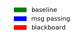
In this section we present experimental results for graph clustering in the message passing and blackboard models. We will compare the following three algorithms. (1) Baseline: each site sends all the data to the coordinator directly; (2) MsgPassing: our algorithm in the message passing model (Section 3.1); (3) Blackboard: our algorithm in the blackboard model (Section 3.2).

Besides giving the visualized results of these algorithms on various datasets, we also measure the qualities of the results via the normalized cut, defined as

$$\text{ncut}(A_{1},\ldots,A_{k})=\frac{1}{2}\sum_{i\in[k]}\frac{w(A_{i},V\backslash A_{i})}{\mu(A_{i})},$$

which is a standard objective function to be minimized for spectral clustering algorithms.

We implemented the algorithms using multiple languages, including Matlab, Python and C++. Our experiments were conducted on an IBM NeXtScale nx360 M4 server, which is equipped with 2 Intel Xeon E5-2652 v2 8-core processors, 32GB RAM and 250GB local storage.

5.1 Datasets.

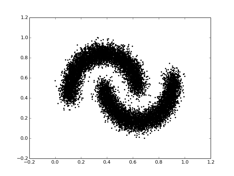
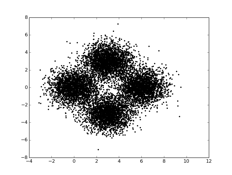
We test the algorithms in the following real and synthetic datasets, which is visualized in Figure 1.

(a) Twomoons

(b) Gauss

(c) Sculpture

Figure 1: Visualization of the datasets for our experiments.

• Twomoons: this dataset contains $n=14,000$ coordinates in $\mathbb{R}^{2}$. We consider each point to be a vertex. For any two vertices $u,v$, we add an edge with weight $w(u,v)=\exp\{-\|u-v\|_{2}^{2}/\sigma^{2}\}$ with $\sigma=0.1$ when one vertex is among the $7000$-nearest points of the other. This construction results in a graph with about $110,000,000$ edges.

• Gauss: this dataset contains $n=10,000$ points in $\mathbb{R}^{2}$. There are $4$ clusters in this dataset, each generated using a Gaussian distribution. We construct a complete graph as the similarity graph. For any two vertices $u,v$, we define the weight $w(u,v)=\exp\{-\|u-v\|_{2}^{2}/\sigma^{2}\}$ with $\sigma=1$. The resulting graph has about $100,000,000$ edges.

• Sculpture: a photo of The Greek Slave . We use an $80\times 150$ version of this photo where each pixel is viewed as a vertex. To construct a similarity graph, we map each pixel to a point in $\mathbb{R}^{5}$, i.e., $(x,y,r,g,b)$, where the latter three coordinates are the RGB values. For any two vertices $u,v$, we put an edge between $u,v$ with weight $w(u,v)=\exp\{-\|u-v\|_{2}^{2}/\sigma^{2}\}$ with $\sigma=0.5$ if one of $u,v$ is among the $5000$-nearest points of the other. This results in a graph with about $70,000,000$ edges.

In the distributed model edges are randomly partitioned across $s$ sites.

5.2 Results on clustering quality

(a) Baseline

(b) MsgPassing

(c) Blackboard

Twomoons, $k=2$;

(d) Baseline

(e) MsgPassing

(f) Blackboard

Gauss, $k=4$

(g) Baseline

(h) MsgPassing

(i) Blackboard

Sculpture, $k=3$.

Figure 2: Visualization of the results on Twomoons, Gauss and Sculpture. In the message passing model each site samples $5n$ edges; in the blackboard model all sites jointly sample $10n$ edges (in Twomoons  and Gauss) or $20n$ edges (in Sculpture) and the chain has length $18$. $s=15$.

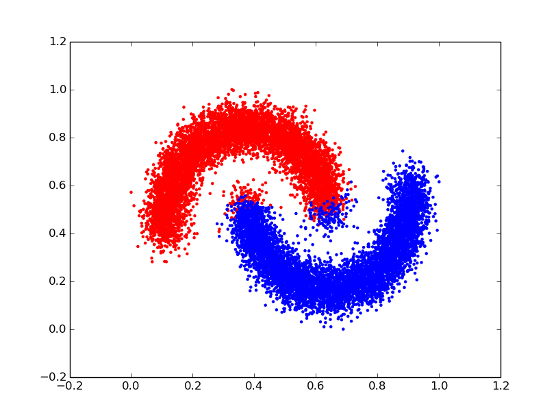
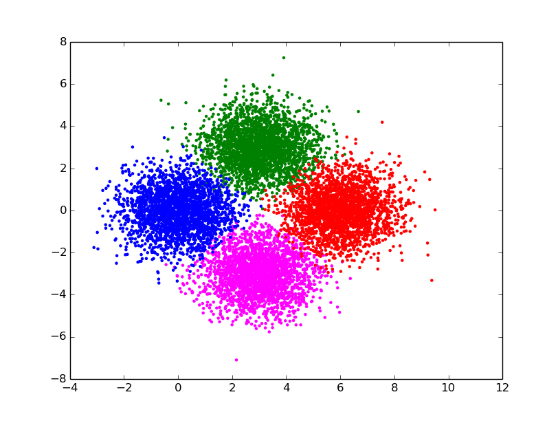
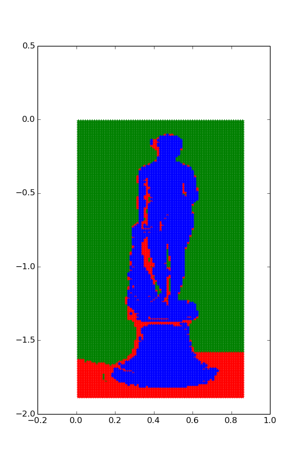
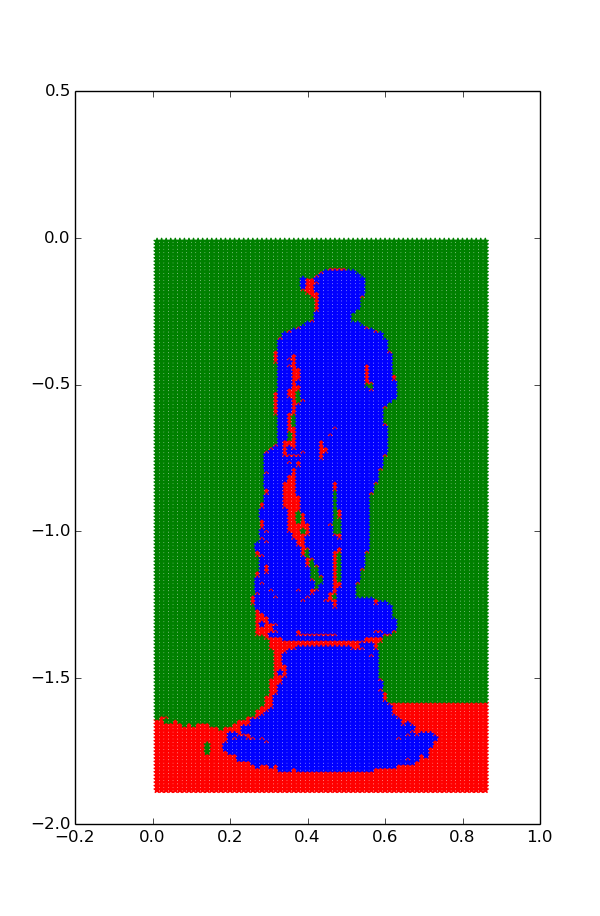
We visualize the clustered results for the Twomoons, Gauss and Sculpture in Figure 2. It can be seen that Baseline, MsgPassing and Blackboard give results of very similar qualities. For simplicity, here we only present the visualization for $s=15$. Similar results were observed when we varied the values of $s$.

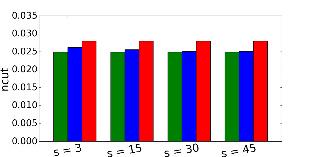
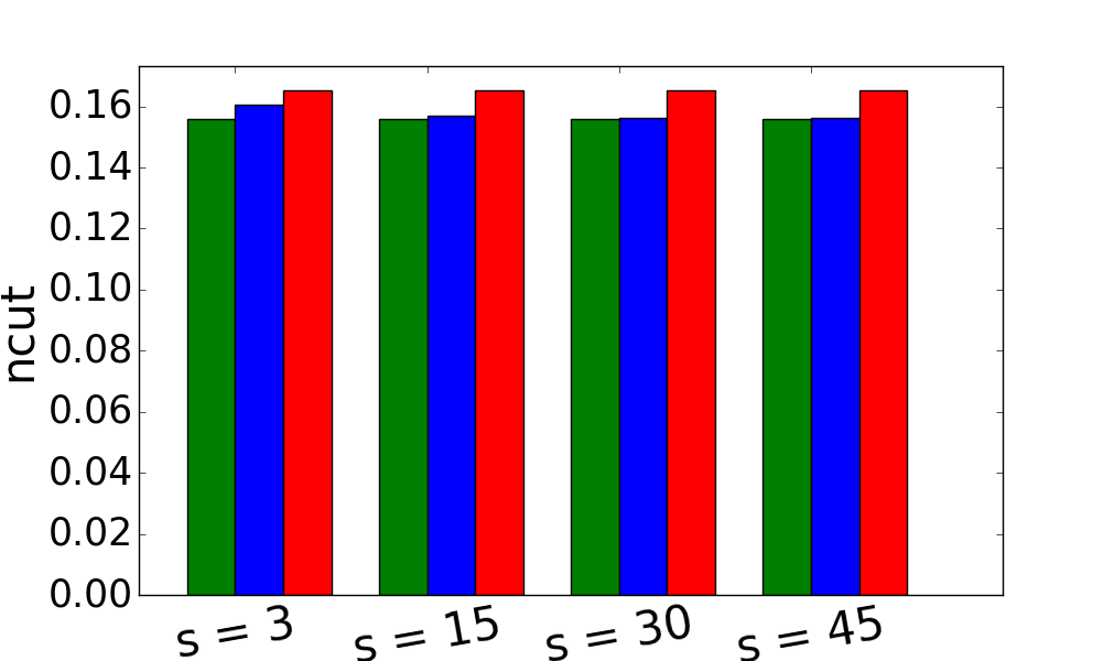
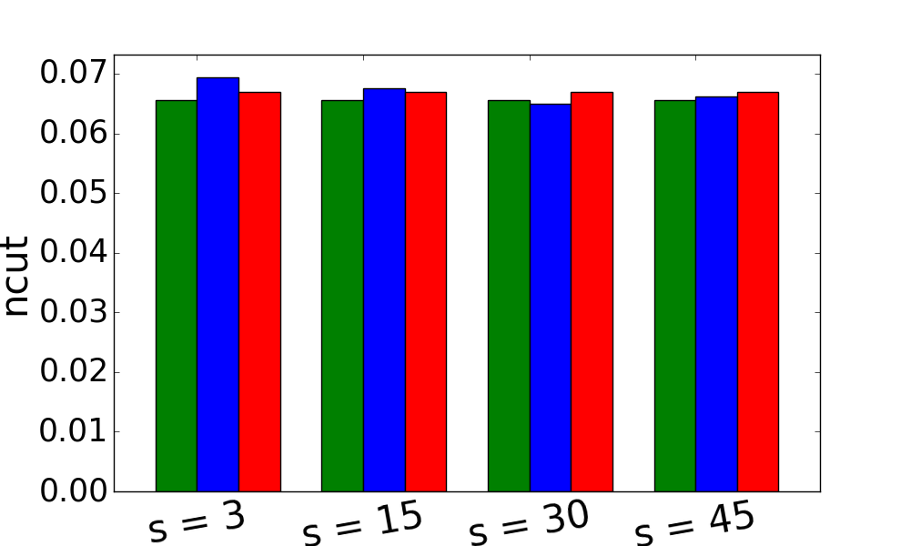
We also compare the normalized cut (ncut) values of the clustering results of different algorithms. The results are presented in Figure 3. In all datasets, the ncut values of different algorithms are very close. The ncut value of MsgPassing slightly decreases when we increase the value of $s$, while the ncut value of Blackboard is independent of $s$.

(a) Twomoons

(b) Gauss

(c) Sculpture

Figure 3: Comparisons on normalized cuts. In the message passing model, each site samples $5n$ edges; in each round of the algorithm in the blackboard model, all sites jointly sample $10n$ edges (in Twomoons and Gauss) or $20n$ edges (in Sculpture) edges and the chain has length $18$.

5.3 Results on communication costs

(a) Twomoons

(b) Gauss

(c) Sculpture

(d) Twomoons

(e) Gauss

(f) Sculpture

Figure 4: Comparisons on communication costs. In the message passing model, each site samples $5n$ edges; in each round of the algorithm in the blackboard model, all sites jointly sample $10n$ (in Twomoons and Gauss) or $20n$ (in Sculpture) edges and the chain has length $18$.

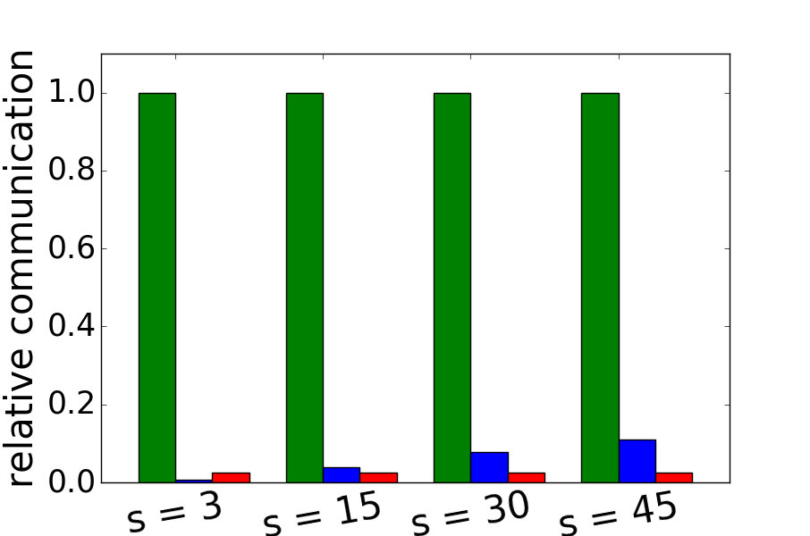
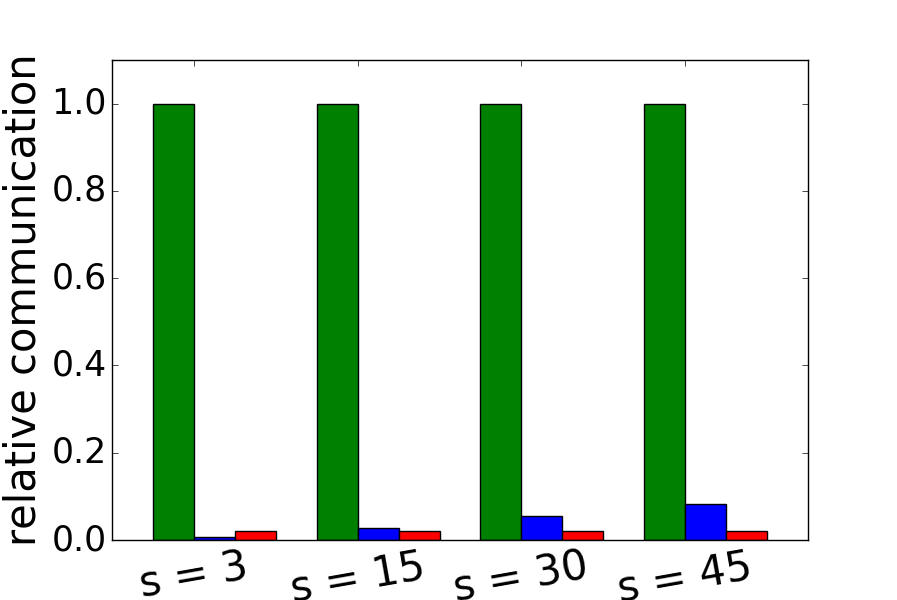
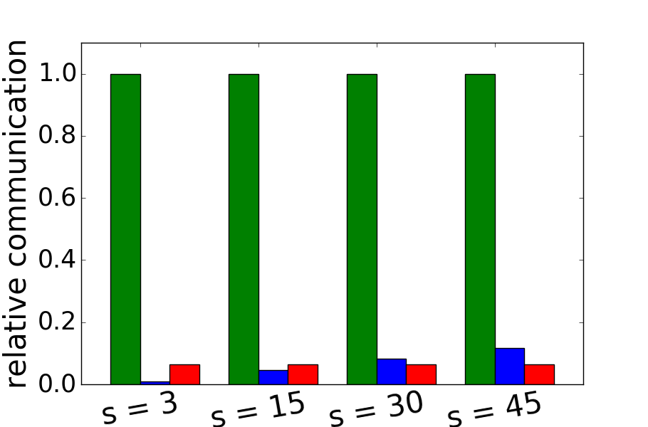
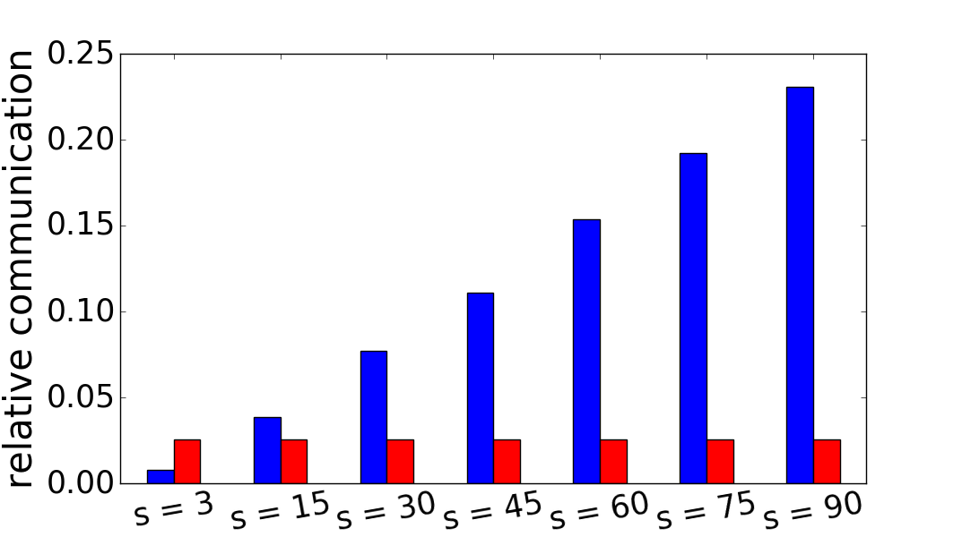
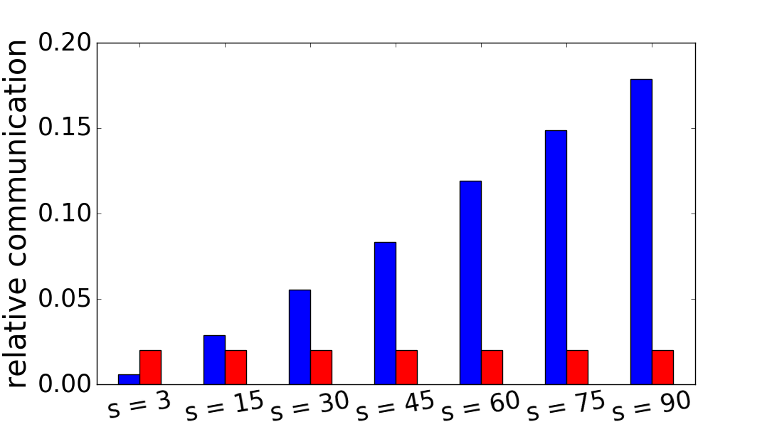
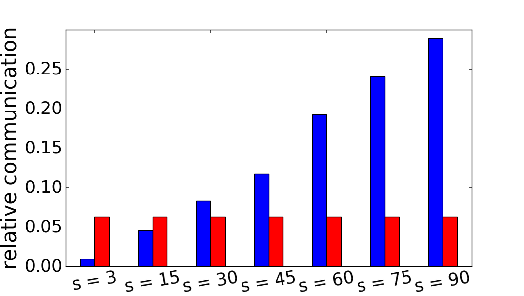
We compare the communication costs of different algorithms in Figure 4. We observe that while achieving similar clustering qualities as Baseline, both MsgPassing and Blackboard are significantly more communication-efficient (by one or two orders of magnitudes in our experiments). We also notice that the value of $s$ does not affect the communication cost of Blackboard, while the communication cost of MsgPassing grows almost linearly with $s$; when $s$ is large, MsgPassing uses significantly more communication than Blackboard. These confirm our theory.

5.4 Parameters in MsgPassing and Blackboard

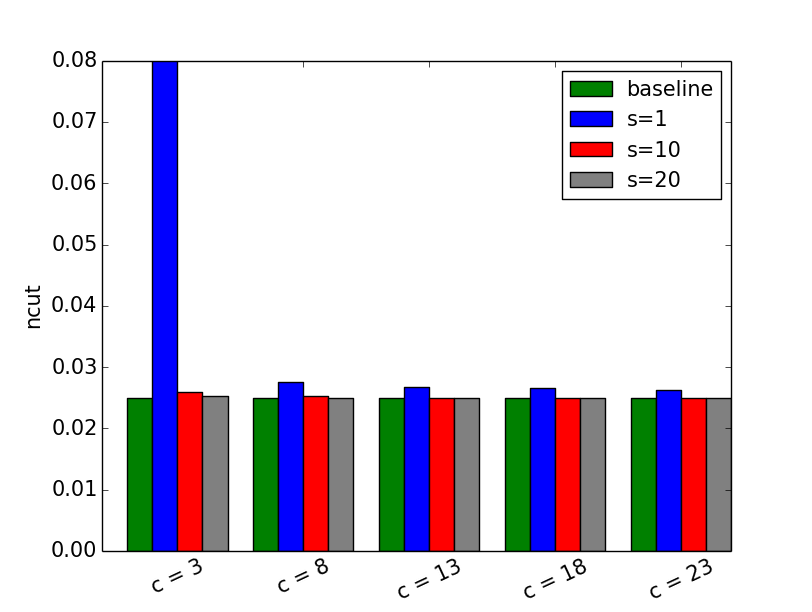
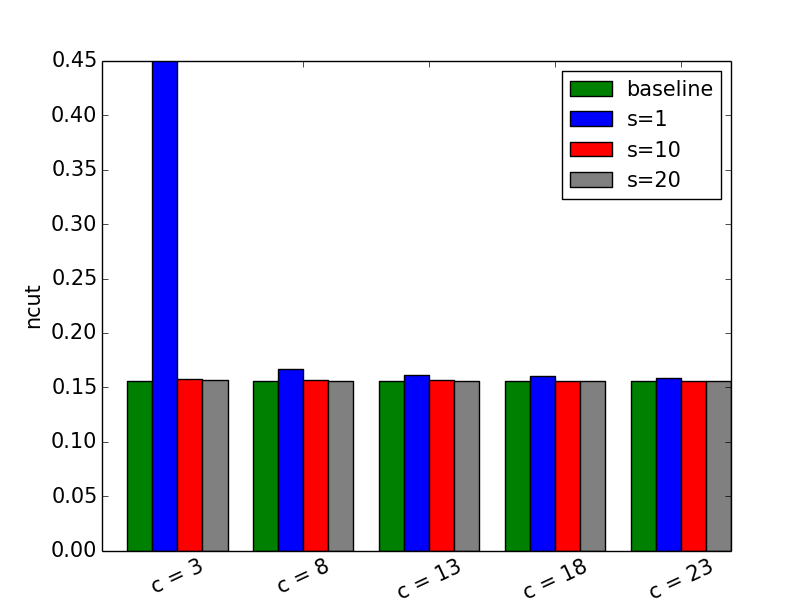
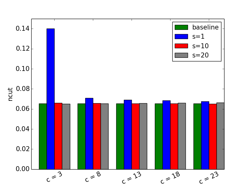
Figure 5 shows in MsgPassinghow the value of ncut is affected by the number of sites and the number of edges sampled in each site. Here, each site samples $cn$ edges. When $c=3$ and $s=1$, the ncut value diverges in all datasets. This is because with such a small $c$, the algorithm does not generate a valid sparsifier. In general, increasing $c$ or $s$ will slightly decrease the ncut value. But once they are above some thresholds, the ncut values of MsgPassing and Baseline become very close.

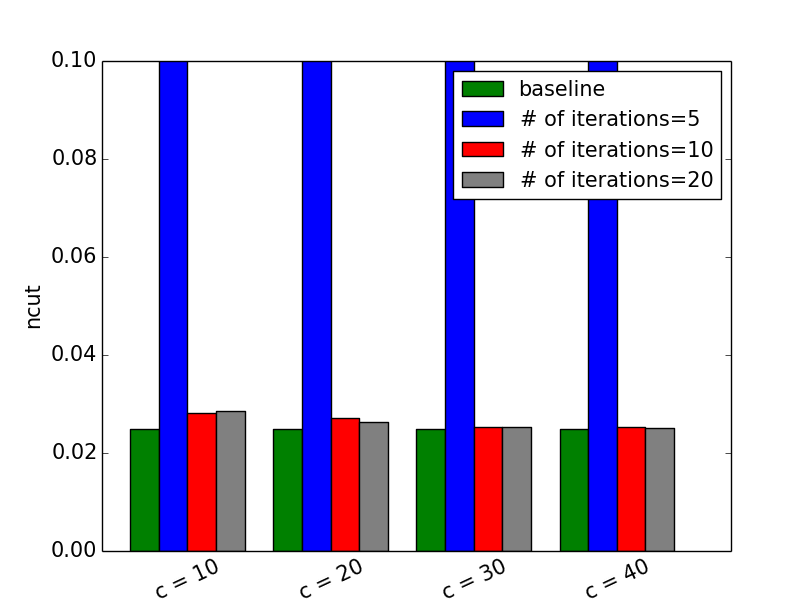
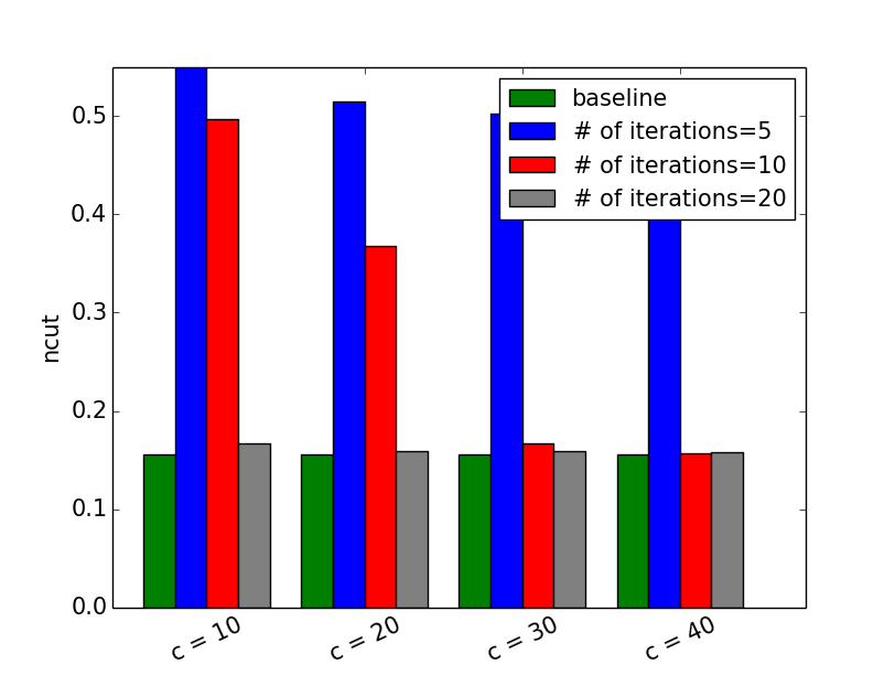
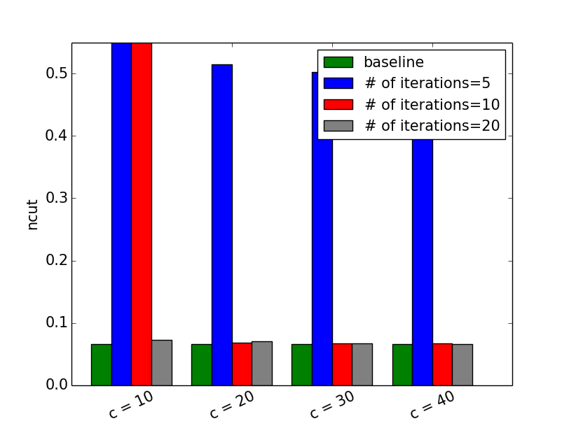
Figure 6 shows in Blackboardhow the ncut value is affected by the number of iterations and the number of edges sampled. When the number of iterations is set to be $5$, ncut values diverge in all datasets. This is because we cannot expect to generate a valid sparsifier by using such few iterations. It can be seen from 6(b) that for a fixed $c$, performing more iterations will help to reduce ncut values. From the same figure, one can also conclude that for fixed iterations, increasing $c$ also helps to reduce the ncut values.

(a) Twomoons

(b) Gauss dataset

(c) Sculpture

Figure 5: The pictures above show the ncut values with respect to the values of $c$ and $s$ for the MsgPassing algorithm. Here each site samples $cn$ edges.

(a) Twomoons

(b) Gauss

(c) Sculpture

Figure 6: The pictures above show how the ncut values are affected by the number of iterations and the value of $c$ for the Blackboard algorithm. Here all sites jointly sample $cn$ edges.

References

- [1] Alexandr Andoni, Jiecao Chen, Robert Krauthgamer, Bo Qin, David P. Woodruff, and Qin Zhang. On sketching quadratic forms. In ITCS, pages 311–319, 2016.
- [2] David Arthur and Sergei Vassilvitskii. -means++: The advantages of careful seeding. In SODA, pages 1027–1035, 2007.
- [3] Maria-Florina Balcan, Steven Ehrlich, and Yingyu Liang. Distributed -means and -median clustering on general communication topologies. In NIPS, pages 1995–2003, 2013.
- [4] Maria-Florina Balcan, Vandana Kanchanapally, Yingyu Liang, and David P. Woodruff. Improved distributed principal component analysis. CoRR, abs/1408.5823, 2014.
- [5] Mark Braverman, Faith Ellen, Rotem Oshman, Toniann Pitassi, and Vinod Vaikuntanathan. A tight bound for set disjointness in the message-passing model. In FOCS, pages 668–677, 2013.
- [6] Moses Charikar, Samir Khuller, David M. Mount, and Giri Narasimhan. Algorithms for facility location problems with outliers. In SODA, pages 642–651, 2001.
- [7] Michael B. Cohen, Sam Elder, Cameron Musco, Christopher Musco, and Madalina Persu. Dimensionality reduction for -means clustering and low rank approximation. In STOC, pages 163–172, 2015.
- [8] Graham Cormode, S. Muthukrishnan, Ke Yi, and Qin Zhang. Continuous sampling from distributed streams. J. ACM, 59(2):10, 2012.
- [9] Graham Cormode, S Muthukrishnan, and Wei Zhuang. Conquering the divide: Continuous clustering of distributed data streams. In ICDE, pages 1036–1045, 2007.
- [10] Dan Feldman, Melanie Schmidt, and Christian Sohler. Turning big data into tiny data: Constant-size coresets for k-means, PCA and projective clustering. In SODA, pages 1434–1453, 2013.
- [11] Sudipto Guha, Yi Li, and Qin Zhang. Distributed partial clustering. Manuscript, 2017.
- [12] Zengfeng Huang, Bozidar Radunovic, Milan Vojnovic, and Qin Zhang. Communication complexity of approximate matching in distributed graphs. In STACS, pages 460–473, 2015.
- [13] Madhukar R. Korupolu, C. Greg Plaxton, and Rajmohan Rajaraman. Analysis of a local search heuristic for facility location problems. In SODA, pages 1–10, 1998.
- [14] James R. Lee, Shayan Oveis Gharan, and Luca Trevisan. Multi-way spectral partitioning and higher-order cheeger inequalities. In STOC, pages 1117–1130, 2012.
- [15] Yin Tat Lee and He Sun. Constructing linear-sized spectral sparsification in almost-linear time. In FOCS, pages 250–269, 2015.
- [16] Zvi Lotker, Elan Pavlov, Boaz Patt-Shamir, and David Peleg. MST construction in communication rounds. In SPAA, pages 94–100, 2003.
- [17] Ramgopal R. Mettu and C. Greg Plaxton. Optimal time bounds for approximate clustering. Machine Learning, 56(1-3):35–60, 2004.
- [18] Gary L. Miller and Richard Peng. Iterative approaches to row sampling. CoRR, abs/1211.2713, 2012.
- [19] Andrew Y. Ng, Michael I. Jordan, and Yair Weiss. On spectral clustering: Analysis and an algorithm. Advances in neural information processing systems, 2:849–856, 2002.
- [20] Richard Peng, He Sun, and Luca Zanetti. Partitioning well-clustered graphs: Spectral clustering works! In COLT, pages 1423–1455, 2015.
- [21] Jeff M. Phillips, Elad Verbin, and Qin Zhang. Lower bounds for number-in-hand multiparty communication complexity, made easy. SIAM J. Comput., 45(1):174–196, 2016.
- [22] Ulrike Von Luxburg. A tutorial on spectral clustering. Statistics and computing, 17(4):395–416, 2007.
- [23] David P. Woodruff and Qin Zhang. Tight bounds for distributed functional monitoring. In STOC, pages 941–960, 2012.