Design, Analysis and Application of A Volumetric Convolutional Neural Network

Abstract

The design, analysis and application of a volumetric convolutional neural network (VCNN) are studied in this work. Although many CNNs have been proposed in the literature, their design is empirical. In the design of the VCNN, we propose a feed-forward K-means clustering algorithm to determine the filter number and size at each convolutional layer systematically. For the analysis of the VCNN, the cause of confusing classes in the output of the VCNN is explained by analyzing the relationship between the filter weights (also known as anchor vectors) from the last fully-connected layer to the output. Furthermore, a hierarchical clustering method followed by a random forest classification method is proposed to boost the classification performance among confusing classes. For the application of the VCNN, we examine the 3D shape classification problem and conduct experiments on a popular ModelNet40 dataset. The proposed VCNN offers the state-of-the-art performance among all volume-based CNN methods.

1 Introduction

3D shape classification [1] is an important yet challenging task arising in recent years. Larger repositories of 3D models [2] such as google sketchup and Yobi 3D have been built for many applications. They include 3D printing, game design, mechanical manufacture, medical analysis, and so on. To handle the increasing size of repositories, an accurate 3D shape classification system is in demand.

Quite a few hand-craft features [3], [4], [5] were proposed to solve the 3D shape classification problem before. Interesting properties of a 3D model are explored from different representations such as views [6], [7], [8], volumetric data [9], [10], [11], and mesh models [12], [13], [14], [15]. However, these features are not discriminative enough to overcome large intra-class variation and strong inter-class similarity. In recent years, solutions based on the convolutional neural network (CNN) [16], [17] have been developed for numerous computer vision applications with significantly better performances. As evidenced by recent publications [18], [19], [20], the CNN solutions also outperform traditional methods relying on hand-craft features in the 3D shape classification problem.

A CNN method classifies 3D shapes using either view-based [21], [22] or volume-based input data [23], [24], [25]. A view-based CNN classifies 3D shapes by analyzing multiple rendered views while a volume-based CNN conducts classification directly in the 3D representation. Currently, the classification performance of the view-based CNN is better than that of the volume-based CNN since the resolution of the volumetric input data has to be much lower than that of the view-based input data due to higher memory and computational requirements of the volumetric input. On the other hand, since volume-based methods preserve the 3D structural information, it is expected to have a greater potential in the long run.

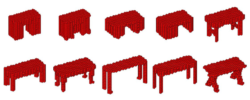
(a) Desk and table

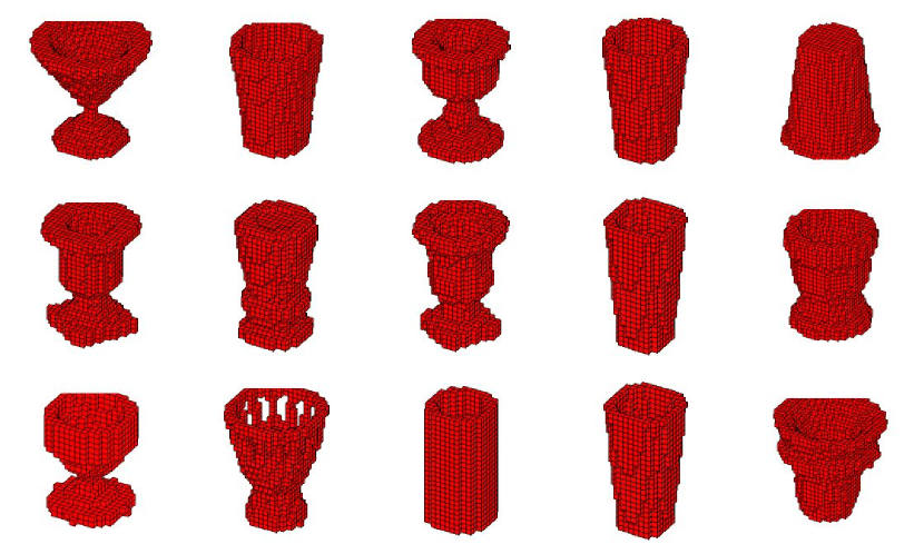
(b) Cup, flower pot and vase

Figure 1: Two sets of confusing classes: (a) desks (the first row) and tables (the second row), and (b) cups (the first row), flower pots (second row) and vases (third row). The confusion is attributed to the similar global appearance of these 3D shapes.

In this work, we target at shrinking the performance gap between volume-based CNN methods and view-based CNN methods, and call the resulting solution the “Volumetric CNN” or VCNN in short. Furthermore, we attempt to conduct fundamental research on network design and understanding in the following two aspects.

1. The VCNN architecture is similar to that of the VoxNet [23]. In traditional CNN design, the network parameters are chosen empirically with high computational complexity. Here, we determine the VCNN network parameters with theoretic support. Specifically, we propose a feed-forward K-means clustering algorithm to identify the optimal filter number and the filter size systematically.

2. Being similar to any other real world classification problem, there exist sets of confusing classes in the 3D shape classification problem [26]. We propose a method to determine whether two shape classes could be confusing based on the network property alone. To enhance the classification performance among confusing classes, we propose a hierarchical clustering method to split samples of the same confusion set into multiple subsets. Then, samples in a subset are reclassified using a random forest (RF) classifier.

To illustrate the second point above, we show two confusion sets in Fig. 1. It will be argued that the filter weights that connect the last fully connected (FC) layer and the output layer carry very valuable information. It points to the centroid of feature vectors of shapes in the same class, and is therefore called the ”shape anchor vector” (SAV) for the class. Two shape classes are confusing if the angle of their SAVs is small and at least one of them has a large inter-class variance (or diversity).

The rest of this paper is organized as follows. Related work is reviewed in Sec. 2. The proposed VCNN system is presented in Sec. 3. Experimental results are given to demonstrate the superior performance of the VCNN method in Sec. 4. Finally, concluding remarks are given in Sec. 5.

2 Related Work

There are two main approaches proposed to classify 3D shape models: the view-based approach and the volume-based approach. They are reviewed below. The view-based approach renders a 3D shape into multiple views as the representation. Classifying a 3D shape becomes analyzing a bundle of views collectively. The Multi-View Convolutional Neural Network (MVCNN) [22] method renders a 3D shape into 12 or 80 views. By adding a view-pooling layer in the VGG network model [27], views of the input shape are merged before the fully connected layers to identify salient regions and overcome the rotational variance. The DeepPano [21] method constructs panoramic views for a 3D shape. A row-wise max-pooling layer is proposed to remove the shift variance. The MVCNN-Sphere method [24] builds a resolution pyramid for each view using sphere rendering based on the MVCNN structure. The classification performance is improved by combining decisions from inputs of different resolutions. View-based methods can preserve the high resolution of 3D shapes since they leverage the view projection and lower the complexity from 3D to 2D. Furthermore, a view-based CNN can be fine-tuned from a pretrained CNN that was trained by 2D images. However, the view-based CNN has two potential shortcomings. First, the surface of a 3D shape can be affected by the shading effect. Second, reconstructing the relationship among views is difficult since the 3D information is lost after the view-pooling process.

The volume-based approach voxelizes a 3D mesh model for a 3D representation. Several CNN networks have been proposed to classify the 3D shapes directly. Examples include the 3D ShapeNet [25], the VoxNet [23] and the SubVolume supervision method [24]. Although the network architectures of volume-based methods are typically shallow (e.g., the VoxNet model consists of two convolutional layers and one fully connected layer), they strike a balance between the number of available training samples and the network model complexity. Volume-based methods have two drawbacks. First, to control computational complexity, the resolution of a 3D voxel model is much lower than that of its corresponding 2D view-based representation. As a result, high frequency components of the original 3D mesh are sacrificed. Second, there are few pretrained CNN models on 3D data, volume-based networks have to be trained from scratch. Although a volumetric representation preserves the 3D structural information of an object, the performance of classifying 3D mesh models directly is still lower than that of classifying the corresponding view-based 2D models.

3 Proposed VCNN Method

3.1 System Overview

An overview of the proposed VCNN solution is shown in Fig. 2. Before the supervised network training phase, we first perform a feed-forward unsupervised clustering procedure to determine the proper size and number of anchor vectors at each layer. Then, in the training phase, the end-to-end backpropagation is conducted, and all filter weights in the network are fine-tuned. The feature vector of the last layer of the VCNN, called the the VCNN feature, is acquired after the training process. Afterwards, a confusion matrix based on SAVs is used to identify confusing sets categorized into pure sets and mixed sets. Each pure set contains a single class of shapes. Each mixed set, which includes multiple classes of samples, is split further into pure subsets and mixed subsets by a proposed tree-structured hierarchical clustering algorithm. Each mixed subset is trained by a random forest classifier. In the testing phase, a sample is assigned to a subset based on its VCNN feature. If the sample is assigned to a pure subset, its label is immediately output. Otherwise, it is assigned to a mixed subset and its label will be determined by the random forest classifier associated with that subset.

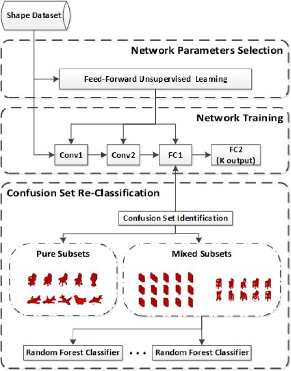
Figure 2: The flow chart of the proposed system

3.2 Shape Anchor Vectors (SAVs)

One key tool adopted in our work is the RECOS (Rectified-COrrelations on a Sphere) model for CNNs as proposed in [28]. The weights of a filter at intermediate layers are interpreted as a cluster centroid of the corresponding inputs. Thus, these weights define an ”anchor vector”. The convolution and nonlinear activation operations at one layer is viewed as projection onto a set of anchor vectors followed by rectification in the RECOS model. The number of anchor filters is related to the approximation capability of a certain layer. The more the number of anchor vectors, the better the approximation capability yet the higher the computational complexity. We will find a way to balance approximation accuracy and computational complexity in Sec. 3.3.

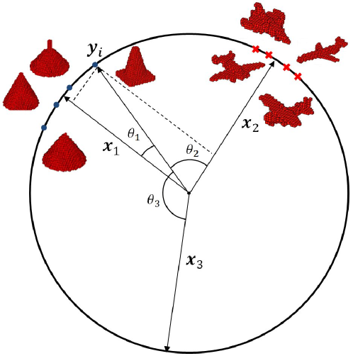
Figure 3: Illustration of anchor vectors at the last stage of a CNN, where each anchor vector points to a 3D shape class. They are called the shape anchor vectors (SAVs). In this example, one SAV points to the airplane class while another SAV points to the cone class.

The anchor vectors at the last stage of a CNN connect the last FC layer to the output. They have a special physical meaning as shown in Fig. 3, where each anchor vector points to a 3D shape class. Thus, they are called the shape anchor vectors (SAVs). In this example, one SAV points to the airplane class while another SAV points to the cone class. There are four blue dots and four red crosses along the surface of a high-dimensional sphere. They represent the feature vectors of 3D shape samples from the cone and the airplane classes, respectively. The classification of each sample to a particular class is determined by the shortest geodesic distance between the sample and the tip of the SAV of the selected class (or, equivalently, the maximum correlation between the sample vector and the SAV). Thus, sample $y_{i}$ is classified to the cone class as shown in this figure.

The relationship between two SAVs and the sample distribution of a particular class plays a critical role in determining whether two classes are confusing or not. If the angle between two SAVs is small and the samples of a particular class are distributed over a wider range, we will get confusing classes. This will be elaborated in Sec. 3.4.

3.3 Network Parameters Selection

The determination of network parameters such as the filter size and number per layer is often conducted in an ad hoc manner in the current literature. Here, we propose a systematic method to decide these parameters based on a feed-forward unsupervised splitting approach. It consists of two steps: 1) representative sample selection, and 2) representative sample clustering.

Problem Formulation. We can formulate the network design problem as follows. The input to the $j^{th}$ RECOS (or the $j$th convolutional layer) has the following dimension:

$$M^{j-1}\times N^{j-1}\times D^{j-1}\times K^{j-1}.$$

where $M^{j-1}\times N^{j-1}\times D^{j-1}$ are spatial dimensions while $K^{j-1}$ represents the spectral dimension (or the number of anchor vectors) in the previous layer. Its output has the following dimension:

$$M^{j}\times N^{j}\times D^{j}\times K^{j}.$$

Since the $2\times 2\times 2$ to $1\times 1\times 1$ maximum pooling is adopted, we have $M^{j}=0.5M^{j-1},N^{j}=0.5N^{j-1},D^{j}=0.5D^{j-1}.$ Furthermore, the filter from the input to the output has a dimension of

$$m^{j}\times n^{j}\times d^{j}\times K^{j}.$$

We set $m^{j}=n^{j}=d^{j}.$ This is because the input volumetric data is of the cubic shape with the same resolution in all three spatial dimension. Note $(M^{0},N^{0},D^{0},K^{0})=(30,30,30,1)$ is the dimension of the input 3D shape. Given $(M^{j-1},N^{j-1},D^{j-1},K^{j-1})$, the question is how to determine the filter size parameter, $m^{j}$, and the filter number, $K^{j}$.

Representative sample selection. The dimension of the input vector is $m^{j}\times n^{j}\times d^{j}\times K^{j-1}=(m^{j})^{3}\times K^{j-1}$. Let $Y^{j-1}$ denotes the set of all training input samples. However, these input samples are not equally important. Some samples have less discriminant power than others. A good sample selection algorithm can guide the network to learn a more meaningful way to partition the feature space to select more discriminant SAVs for better decisions.

We first normalize all patterns $y^{j-1}\in Y^{j-1}$ to have the unit length. Then, the set $P^{j-1}$ of all normalized inputs can be written as

$$P^{j-1}=\{p^{j-1}\,|\,p^{j-1}=y^{j-1}/||y^{j-1}||,\,y^{j-1}\in Y^{j-1}\}.$$

Next, we adopt the saliency principle in representative pattern selection. That is, we compute the variance of elements in $p^{j-1}$ and choose those of a larger variance value. If the variance of an input is small, it has a flat element-wise distribution and, thus, has a low discriminant power.

We propose a two-stage screening process.In the first stage, a small threshold $\epsilon$ is adopted to remove inputs with very small variance values. That is, if the variance of an input is less than $\epsilon$, it is removed from the candidate sample set. In the second stage, we select top $T\%$ samples with the largest variance values in the filtered candidate sample set to keep all remaining candidates sufficiently salient.

After the above two-stage screening process, we have a smaller candidate sample set that contain salient samples. If we want to reduce the size of the candidate set furthermore to simplify the following computations, a uniform random sampling strategy can be adopted.

Representative sample clustering. Our objective is to find $K^{j}$ anchor vectors from the candidate set of representative samples obtained from the above step. Here, we adopt an unsupervised clustering algorithm such as the K-means algorithm to group them. The cluster centroids are then set to the desired anchor vectors for the current RECOS model.

To choose the optimal parameters, $m^{j}$ and $K^{j}$, we can maximize the inter-cluster margin and minimize the intra-cluster variance by adopting the Bayesian Information Criterion (BIC) function [29]. The approximation of the BIC function in the K-means algorithm can be expressed as

$$BIC(m^{j},K^{j},P^{j-1})=-2\sum_{k_{j}=1}^{K^{j}}{L_{k_{j}}}+2K^{j}C^{j}\log{N},$$ (1)

where $C^{j}=(m^{j})^{3}\times K^{j-1}$ is the dimension of input vectors, $N$ is the total number of elements in $P^{j-1}$, and $L$ is the log-likelihood distance. Under the normal distribution model, we have

$$L_{k_{j}}=-\frac{N_{k_{j}}}{2}\sum_{c_{j}=1}^{C_{j}}\log(\delta_{c_{j}}^{2}+\delta_{c_{j}k_{j}}^{2}),$$ (2)

where $N_{k_{j}}$ is the number of samples in the $k_{j}$th cluster, $\delta_{c_{j}}^{2}$ is the variance of the $c_{j}$th feature variable over all samples, and $\delta_{c_{j}k_{j}}^{2}$ is the variance of the $c_{j}$th feature variable in the $k_{j}$th cluster. By fixing parameter $C_{j}$, the optimal value of $K_{j}$ is determined by detecting the valley point of the BIC function.

The relationship between two consecutive RECOS models is worthy discussion. The problem of selecting optimal parameter pairs, $(m^{j},K^{j})$, across multiple layers is actually inter-dependent. Here, we adopt a greedy algorithm to predict these parameters in a feed-forward manner. The centroids after each K-means clustering serve as the anchor vectors of each RECOS model and they can be used to generate input samples for the next RECOS model.

3.4 Confusion Sets Identification and Re-Classification

In principle, the network parameter selection algorithm presented in the last subsection can be used to decide optimal network parameters for the RECOS models in the leading layers. As the network goes to the end, we need to consider another factor. That is, the number of SAVs in the last layer has to be equal to the number of classes due to the supervised learning framework. The discriminant power of the feature space before the output layer can still be limited and, as a result, SAVs in the last stage may not be able to separate 3D shapes of different classes completely. Then, shapes from different classes can be mixed, leading to confusion sets. In this subsection, we will develop a method to identify these confusion sets. In particular, we would like to address the following two questions: 1) how to split 3D shapes of the same class into multiple sub-classes according to their VCNN features? and 2) what is the relationship between SAVs and visually similar shapes?

Generation of Sub-classes. For the first question, we adopt a tree-structured hierarchical clustering algorithm to split a class into sub-classes, where the class can be either the ground-truth or the predicted one. The algorithm initially splits the feature space into two clusters according to their Euclidean distance by using the K-means algorithm with $K=2$ [30]. Then, for each cluster, the variance is calculated to determine its tightness. A cluster with a large variance is split furthermore. The termination of the splitting process is decided by one of the following two criteria: 1) reaching a sufficiently small variance (say, below threshold $\zeta$), and 2) reaching a sufficiently small size (say, below threshold $\eta$). The number of sub-classes under each class can be automatically determined by the two pre-selected threshold values, $\zeta$ and $\eta$.

(a) Chair

(b) Mantel

(c) Sink

Figure 4: Illustration of 3D shapes in sub-classes obtained from (a) the Chair class, (b) the Mantel class and (c) the Sink class. We provide 16 representative shapes for each sub-class and encircle them with a blue box.

We examine the power of the VCNN features and the tree-structure hierarchical clustering algorithm using the ground-truth label. Results for three classes are shown in Fig. 4. They are chair, mantel and sink. We see that the VCNN features can generate sub-classes that contain visually similar shapes automatically. For example, the chair class can be divided into four sub-classes. They are round chairs, chairs with four feet, wheel chairs and long chairs. The mantel class can be further partitioned into three sub-classes. They are thin mantels, thick mantels and hollow mantels. The sink class can be clustered into four sub-classes; namely, deep sinks, flat sinks, sinks with a hose and table-like sinks. This shows the discriminant power of the VCNN features, which are highly optimized by the backpropagation of the CNN, and the power of the clustering algorithm in identifying intra-class differences.

Confusion Matrix Analysis and Confusion Set Identification. After running samples through the CNN, we will get predicted labels (instead of ground-truth labels). Then, samples of globally similar appearance but from different classes can be mixed in the VCNN feature space. This explains the source of confusion. To resolve confusion among multiple confusing classes, we adopt a merge-and-split strategy. That is, we first merge several confusing classes into one confusion set and, then, split the confusion set into multiple subsets as done before.

We denote the directional confusion score of $i^{th}$ sample, $y_{i}$, to the $k^{th}$ class, $c_{k}$, as $s(y_{i},c_{k})$. Theoretically, it is reciprocal to the projection distance between $y_{i}$ and the SAV of $c_{k}$. By normalizing the projection distances from $y_{i}$ to the SAVs of all classes by using the softmax function, the directional confusion score $s(y_{i},c_{k})$ is equivalent to the soft decision score. The confusion factor (CF) between two classes $c_{k}$ and $c_{l}$ is determined by the average of two directional confusion scores as

$$CF(c_{k},c_{l})=\frac{1}{2N_{k}}\sum_{y_{i}\in c_{k}}s(y_{i},c_{l})+\frac{1}{2N_{l}}\sum_{y_{j}\in c_{l}}s(y_{j},c_{k}),$$ (3)

where $N_{k}$ and $N_{l}$ are the numbers of samples in $c_{k}$ and $c_{l}$, respectively. This CF value can be computed using training samples.

Figure 5: A mixed or pure set is enclosed by a blue box. Each mixed set contains multiple shape classes which are separated by green vertical bars. Two representative 3D shapes are shown for each class. Each row has one mixed set and several pure sets. The mixed set in the first row contains bookshelf, wardrobe, night stand, radio, xbox, dresser and tv stand; that in the second row contains cup, flower pot, lamp, plant and vase; that in the third row contains bench, desk and table; that in the four row contains chair and stool; that in the fifth row contains curtain and door; and that in the six row contains mantel and sink.

Since the confusion matrix defines an affinity matrix, we adopt the spectral clustering algorithm [31] to cluster samples into multiple confusion sets that have strong confusion factors. After the spectral clustering algorithm, we obtain either pure or mixed sets. A pure set contains 3D shapes from the same class. Fig. 5 shows the results of both mixed and pure sets obtained by the confusion matrix analysis. Each confusion set is enclosed by a blue box. Inside a confusion set, each class is represented by two instances. Two different classes are separated by a green bar. Some pure sets are generated because they are isolated from other classes in the clustering process. It is worthwhile to emphasize that each mixed set contains 3D shapes of similar appearance yet under different class labels. For example, the mixed set in the first row contains seven classes: bookshelf, wardrobe, night stand, radio, xbox, dresser and tv stand. All of them are cuboid like.

In the testing phase, if a test sample is classified to a pure set, the class label of that set is output as the desired answer. A mixed set contains 3D shapes from multiple classes, and further processing is needed to separate them. This will be discussed below.

(a)

(b)

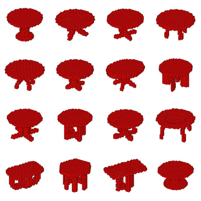
(c)

(d)

(e)

(f)

Figure 6: The split of the confusion set of bench, desk and table yields three pure subsets (a) bench, (b) desk and (c) table and three mixed subsets (d) bench and table, (e) desk and table and (f)bench, desk and table.

(a)

(b)

(c)

(d)

(e)

(f)

Figure 7: The split of the confusion set of lamp, flower pot, cup and vase yields three pure subsets (a) lamp, (b) plant and (c) cup and three mixed subsets (d) flower pot and vase, (e) flower pot and plant and (f) cup, flower pot, lamp, vase.

Confusion Set Re-Classification. We split a confusion set into multiple subsets using the tree-structured hierarchical clustering algorithm. Some of them contain samples from the same class while others still contain samples from multiple classes. They form pure subsets and mixed subsets, respectively. We show splitting results of two confusion sets in Fig. 6 and Fig. 7, respectively. We see from the two figures that shapes in pure subsets are distinctive from other subsets while shapes in the mixed subsets share similar appearances.

To deal with the challenging cases in each mixed subset, we need to train a more effective classifier than the softmax classifier. Furthermore, we have to avoid the potential overfitting problem due to a very limited number of training samples. For the above two reasons, we choose the random forest classifier [32]. Classes are weighted to overcome the unbalance sample distribution for each mixed subset. In the testing phase, a sample is first assigned to a subset based on its VCNN feature using the nearest neighbor rule. If it is assigned to a pure subset, the class label is output as the predicted label. Otherwise, we run the random forest classifier trained for the particular mixed subset to make final class decision.

4 Experimental Results

We test the network parameter selection algorithm and the confusion set re-classification algorithm on the popular dataset ModelNet40 [25]. The ModelNet40 dataset contains 9,843 training samples and 2,468 testing samples categorized into 40 classes. The original mesh model is voxelized into dimension $30\times 30\times 30$ before training and testing. The basic structure of the proposed VCNN is the same as VoxNet [23]: two convolutional layers followed by one fully connected layer. However, we allow to have different filter sizes and filter numbers at these layers.

Results of Network Parameters Selection Alone. We compare the BIC scores with three spatial filter sizes $m^{j}=3,5,7$ in the two convolutional layer. The filter number is chosen to be $K^{j}=$ 32, 64, 128, 256, 512, 768, 1024. For the fully connected layer, the filter number is set to $K^{f}=128,256,512,1024,2048$. We show the BIC scores by adjusting $m^{j}$ and $K^{j}$ at the first convolutional layer in Fig. 8. To keep the BIC scores at the same scale of different filter sizes and training sample numbers, we normalize the BIC function in Eq. 1 by $(m^{j})^{3}$ and keep $N$ independent of $m^{j}$. Three valley points can be easily detected at $(m^{1},K^{1})=(3,256)$, $(5,512)$ and $(7,512)$. This result is reasonable since we need more filters to represent larger spatial patterns. By comparing the three curves, the choice of $(m^{1},K^{1})=(3,256)$ gives the lowest BIC score. By adopting the greedy search algorithm introduced in Section 3.3, the network parameters in all layers of the proposed VCNN are summarized in Table 1. We also include the network parameters of the VoxNet in the table for comparison.

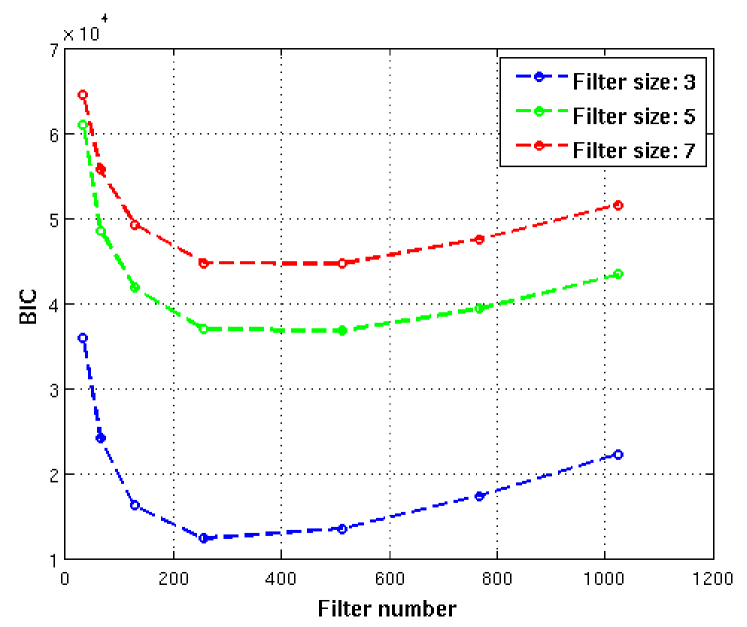
Figure 8: Three BIC curves measured under three different filter sizes $m_{j}=3,5,7$ and seven different filter numbers $K_{j}=32,64,128,256,512,768,1024$ for the first convolutional layer.

Table 1: Comparison of network parameters of the proposed VCNN and the VoxNet, where the numbers in each cell follow the format $(m^{j})^{3}\times K^{j-1}.$

	Conv1	Conv2	FC	Output
VoxNet	$5^{3}\times 1$	$3^{3}\times 32$	$6^{3}\times 32$	$1\times 1\times 128$
Our VCNN	$3^{3}\times 1$	$3^{3}\times 256$	$6^{3}\times 128$	$1\times 1\times 1024$

Table 2: Comparison of ACA and AIA scores of several state-of-the-art methods for the ModelNet40 dataset. Our results are set to bold.

Volume-based methods	ACA	AIA
3DShapeNets[25]	77.30%	-
VoxNet[23]	83.01%	87.40%
3D-Gan [33]	83.30%	-
SubVolume[24]	86.00%	89.20%
AniProbing [24]	85.60%	89.90%
VCNN /wo ReC	85.66%	89.34%
VCNN /w ReC	86.23%	89.78%
View-based methods	ACA	AIA
DeepPano [21]	77.63%	-
GIFT [34]	83.10%	-
MVCNN [22]	90.10%	-
Pairwise [35]	90.70%	-
FusionNet [36]	90.80%	-

Figure 9: Comparison of accuracy per classe between the VoxNet method (blue bars) and our VCNN design (yellow bars).

To compare the performance of the proposed VCNN and other benchmarking methods, we use two performance measures: average class accuracy (ACA) and average instance accuracy (AIA). The ACA score averages the prediction accuracy scores over classes, while the AIA score takes the average of prediction scores over testing samples. The results are shown in Table 2, where methods are classified into the view-based and the volume-based two categories. For the proposed VCNN, we consider two cases: with and without confusion set reclassification. We first focus on the contribution of the network parameters selection algorithm without the confusion set reclassification (w/o ReC) module. The VCNN w/o ReC outperforms the VoxNet by $2.65\%$ and $1.94\%$ in ACA and AIA, respectively. The gap between volume-based and view-based methods is narrowed. Although the ACA performance of the VCNN w/o ReC is lower than that of the SubVolume method by $0.34\%$ and its AIA performance is lower than that of the AniProbing method by $0.56\%$, these two methods use more complex network structures such as multi-orientation pooling and subvolume supervision.

It is worthwhile to examine the classification accuracy for each individual class. We compare the accuracy of the proposed VCNN with that of the VoxNet in Fig. 9. By leveraging the network parameters selection, the performance of most classes is boosted with VCNN. Furthermore, classes of low classification accuracy belong to some confusion sets. The observed results are consistent with those shown in Fig. 5.

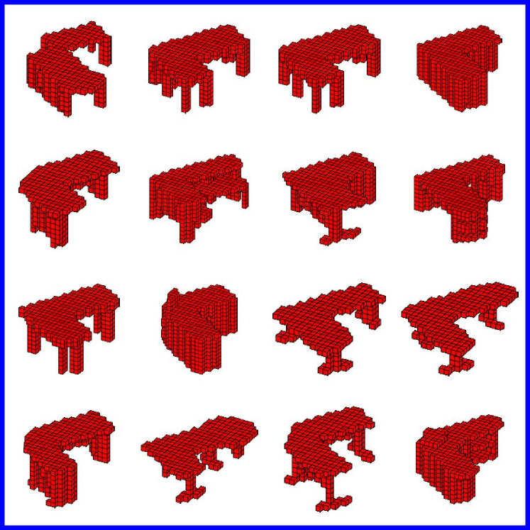
(a) Desk

(b) Lamp

(c) Chair

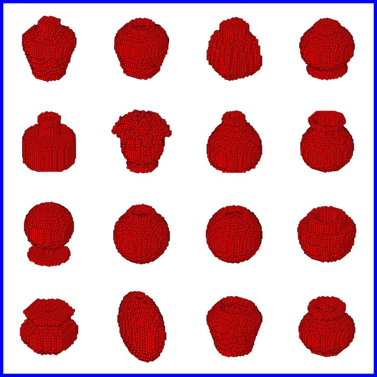
(d) Vase

Figure 10: Four examples of corrected errors: (a) desk, (b) lamp, (c) chair, (d) vase. Each example has a testing sample on the top and its assigned subset on the bottom.

(a) Cup

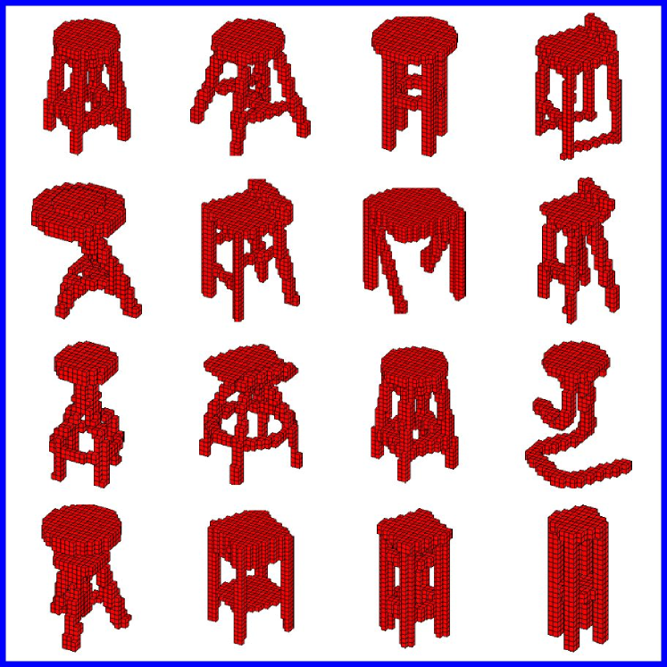
(b) Desk

(c) Dresser

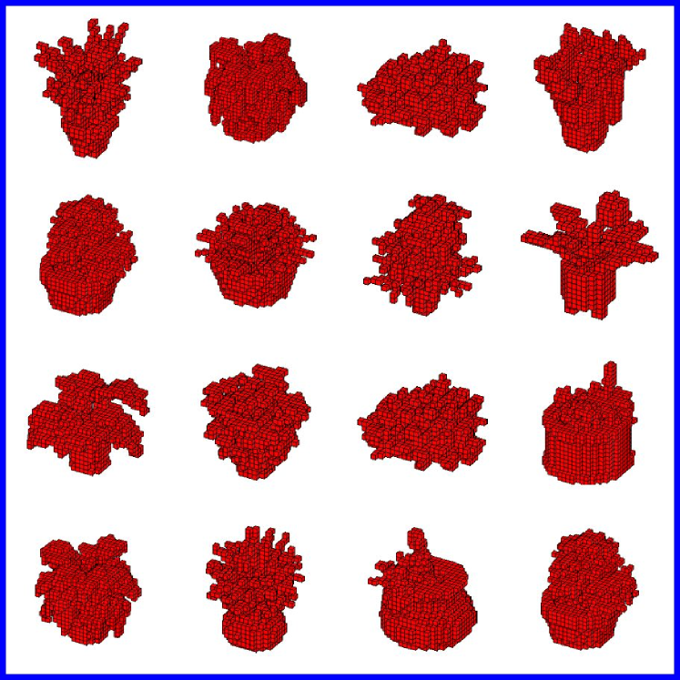
(d) Plant

Figure 11: Four examples of uncorrected errors: (a) cup, (b) desk, (c) dresser, (d) plant. Each example includes a testing sample on the top and the assigned subset on the bottom.

Results of Confusion Set Re-Classification. As shown in Table 2, the classification accuracy can be boosted furthermore by the proposed re-classification algorithm. The improved ACA and AIA values are $0.57\%$ and $0.44\%$. Since the error cases in mixed subsets are difficult cases, such performance gains are good. We observe two cases in the improvement, where wrongly predicted samples can be corrected. First, a sample is assigned to a correct pure subset so that its prediction can be corrected directly. Examples are given in Figs. 10 (a) and (b), where a desk shape and a lamp shape are correctly assigned to one of their pure subsets, respectively. Second, a sample is assigned to a mixed subset and the random forest classifier helps correct the prediction result. Examples are given in Figs. 10 (c) and (d). A chair shape is assigned to a mixed subset containing chairs and stools in Fig. 10 (c). A vase shape is assigned a mixed subset containing flower pots and vases. in Fig. 10 (d). They can be eventually correctly classified using the random forest classifier. The power of the confusion set identification and re-classification procedure is demonstrated by these examples.

Although errors still exist, they can be clearly analyzed based on our clustering results. Uncorrected errors come from the strong feature similarity. In Fig. 11 (a) and (b), a cup shape and a desk shape are wrongly assigned to a mixed subset of vase and flower pot and a mixed subset of chair and stool, respectively. In Fig. 11(c), although a dresser shape is assigned to a mixed subset containing dressers, night stands, radio, tv stands and wardrobe, the VCNN features are not distinctive enough to produce a correct classification. Similarly in Fig. 11 (d), a plant shape cannot be differentiated from the flower pot in its mixed subset. These mistakes are due to their highly visual similarity with shapes in other classes. Additionally, the success of our confusion set identification algorithm offers the possibility of using more advanced methods (e.g., a part-based classifier [37]) to improve the classification performance on erroneous samples. A higher classification accuracy is expected in the future.

5 Conclusion

The design, analysis and application of a volumetric convolutional neural network (VCNN) were presented. We proposed a feed-forward K-means clustering algorithm to determine the filter number and size. The cause of confusion sets was identified. Furthermore, a hierarchical clustering method followed by a random forest classification method was proposed to boost the classification performance among confusing classes. Finally, experiments were conducted on a popular ModelNet40 dataset. The proposed VCNN offers the state-of-the-art performance among all volume-based CNN methods.

References

- [1] P. Shilane, P. Min, M. Kazhdan, T. Funkhouser, The princeton shape benchmark, in: Shape modeling applications, 2004. Proceedings, IEEE, 2004, pp. 167–178.
- [2] S. Spaeth, P. Hausberg, Can open source hardware disrupt manufacturing industries? the role of platforms and trust in the rise of 3d printing, in: The Decentralized and Networked Future of Value Creation, Springer, 2016, pp. 59–73.
- [3] B. Li, A. Godil, M. Aono, X. Bai, T. Furuya, L. Li, R. J. López-Sastre, H. Johan, R. Ohbuchi, C. Redondo-Cabrera, et al., Shrec’12 track: Generic 3d shape retrieval., in: 3DOR, 2012, pp. 119–126.
- [4] B. Li, Y. Lu, C. Li, A. Godil, T. Schreck, M. Aono, M. Burtscher, Q. Chen, N. K. Chowdhury, B. Fang, et al., A comparison of 3d shape retrieval methods based on a large-scale benchmark supporting multimodal queries, Computer Vision and Image Understanding 131 (2015) 1–27.
- [5] J. W. Tangelder, R. C. Veltkamp, A survey of content based 3d shape retrieval methods, Multimedia tools and applications 39 (3) (2008) 441–471.
- [6] M. Chaouch, A. Verroust-Blondet, A new descriptor for 2d depth image indexing and 3d model retrieval, in: 2007 IEEE International Conference on Image Processing, Vol. 6, IEEE, 2007, pp. VI–373.
- [7] D.-Y. Chen, X.-P. Tian, Y.-T. Shen, M. Ouhyoung, On visual similarity based 3d model retrieval, in: Computer graphics forum, Vol. 22, Wiley Online Library, 2003, pp. 223–232.
- [8] R. Ohbuchi, K. Osada, T. Furuya, T. Banno, Salient local visual features for shape-based 3d model retrieval, in: Shape Modeling and Applications, 2008. SMI 2008. IEEE International Conference on, IEEE, 2008, pp. 93–102.
- [9] M. Kazhdan, T. Funkhouser, S. Rusinkiewicz, Rotation invariant spherical harmonic representation of 3 d shape descriptors, in: Symposium on geometry processing, Vol. 6, 2003, pp. 156–164.
- [10] M. Novotni, R. Klein, Shape retrieval using 3d zernike descriptors, Computer-Aided Design 36 (11) (2004) 1047–1062.
- [11] H. Sundar, D. Silver, N. Gagvani, S. Dickinson, Skeleton based shape matching and retrieval, in: Shape Modeling International, 2003, IEEE, 2003, pp. 130–139.
- [12] A. M. Bronstein, M. M. Bronstein, L. J. Guibas, M. Ovsjanikov, Shape google: Geometric words and expressions for invariant shape retrieval, ACM Transactions on Graphics (TOG) 30 (1) (2011) 1.
- [13] M. M. Bronstein, I. Kokkinos, Scale-invariant heat kernel signatures for non-rigid shape recognition, in: Computer Vision and Pattern Recognition (CVPR), 2010 IEEE Conference on, IEEE, 2010, pp. 1704–1711.
- [14] R. Gal, A. Shamir, D. Cohen-Or, Pose-oblivious shape signature, IEEE transactions on visualization and computer graphics 13 (2) (2007) 261–271.
- [15] D. Smeets, J. Keustermans, D. Vandermeulen, P. Suetens, meshsift: Local surface features for 3d face recognition under expression variations and partial data, Computer Vision and Image Understanding 117 (2) (2013) 158–169.
- [16] A. Krizhevsky, I. Sutskever, G. E. Hinton, Imagenet classification with deep convolutional neural networks, in: Advances in neural information processing systems, 2012, pp. 1097–1105.
- [17] Y. LeCun, Y. Bengio, G. Hinton, Deep learning, Nature 521 (7553) (2015) 436–444.
-
[18]
A. X. Chang, T. A. Funkhouser, L. J. Guibas, P. Hanrahan, Q. Huang, Z. Li,
S. Savarese, M. Savva, S. Song, H. Su, J. Xiao, L. Yi, F. Yu,
Shapenet: An information-rich 3d model
repository, CoRR abs/1512.03012.
URL http://arxiv.org/abs/1512.03012 - [19] M. Savva, F. Yu, H. Su, M. Aono, B. Chen, D. Cohen-Or, W. Deng, H. Su, S. Bai, X. Bai, et al., Shrec’16 track large-scale 3d shape retrieval from shapenet core55.
- [20] J. Xie, Y. Fang, F. Zhu, E. Wong, Deepshape: Deep learned shape descriptor for 3d shape matching and retrieval, in: Proceedings of the IEEE Conference on Computer Vision and Pattern Recognition, 2015, pp. 1275–1283.
- [21] B. Shi, S. Bai, Z. Zhou, X. Bai, Deeppano: Deep panoramic representation for 3-d shape recognition, IEEE Signal Processing Letters 22 (12) (2015) 2339–2343.
- [22] H. Su, S. Maji, E. Kalogerakis, E. Learned-Miller, Multi-view convolutional neural networks for 3d shape recognition, in: Proceedings of the IEEE International Conference on Computer Vision, 2015, pp. 945–953.
- [23] D. Maturana, S. Scherer, Voxnet: A 3d convolutional neural network for real-time object recognition, in: Intelligent Robots and Systems (IROS), 2015 IEEE/RSJ International Conference on, IEEE, 2015, pp. 922–928.
- [24] C. R. Qi, H. Su, M. Niessner, A. Dai, M. Yan, L. J. Guibas, Volumetric and multi-view cnns for object classification on 3d data, arXiv preprint arXiv:1604.03265.
- [25] Z. Wu, S. Song, A. Khosla, F. Yu, L. Zhang, X. Tang, J. Xiao, 3d shapenets: A deep representation for volumetric shapes, in: Proceedings of the IEEE Conference on Computer Vision and Pattern Recognition, 2015, pp. 1912–1920.
- [26] J. Dong, Q. Chen, J. Feng, K. Jia, Z. Huang, S. Yan, Looking inside category: subcategory-aware object recognition, IEEE Transactions on Circuits and Systems for Video Technology 25 (8) (2015) 1322–1334.
- [27] K. Simonyan, A. Zisserman, Very deep convolutional networks for large-scale image recognition, CoRR abs/1409.1556.
-
[28]
C. J. Kuo, Understanding convolutional
neural networks with A mathematical model, CoRR abs/1609.04112.
URL http://arxiv.org/abs/1609.04112 - [29] D. Pelleg, A. W. Moore, et al., X-means: Extending k-means with efficient estimation of the number of clusters., in: ICML, Vol. 1, 2000.
- [30] J. A. Hartigan, M. A. Wong, Algorithm as 136: A k-means clustering algorithm, Journal of the Royal Statistical Society. Series C (Applied Statistics) 28 (1) (1979) 100–108.
- [31] A. Y. Ng, M. I. Jordan, Y. Weiss, et al., On spectral clustering: Analysis and an algorithm, Advances in neural information processing systems 2 (2002) 849–856.
- [32] L. Breiman, Random forests, Machine learning 45 (1) (2001) 5–32.
- [33] J. Wu, C. Zhang, T. Xue, W. T. Freeman, J. B. Tenenbaum, Learning a probabilistic latent space of object shapes via 3d generative-adversarial modeling, arXiv preprint arXiv:1610.07584.
- [34] S. Bai, X. Bai, Z. Zhou, Z. Zhang, L. J. Latecki, Gift: A real-time and scalable 3d shape search engine, arXiv preprint arXiv:1604.01879.
- [35] E. Johns, S. Leutenegger, A. J. Davison, Pairwise decomposition of image sequences for active multi-view recognition, arXiv preprint arXiv:1605.08359.
- [36] V. Hegde, R. Zadeh, Fusionnet: 3d object classification using multiple data representations, arXiv preprint arXiv:1607.05695.
- [37] N. Zhang, J. Donahue, R. Girshick, T. Darrell, Part-based r-cnns for fine-grained category detection, in: European conference on computer vision, Springer, 2014, pp. 834–849.