Spatio-temporal canards in neural field equations

Abstract

Canards are special solutions to ordinary differential equations that follow invariant repelling slow manifolds for long time intervals. In realistic biophysical single cell models, canards are responsible for several complex neural rhythms observed experimentally, but their existence and role in spatially-extended systems is largely unexplored. We describe a novel type of coherent structure in which a spatial pattern displays temporal canard behavior. Using interfacial dynamics and geometric singular perturbation theory, we classify spatio-temporal canards and give conditions for the existence of folded-saddle and folded-node canards. We find that spatio-temporal canards are robust to changes in the synaptic connectivity and firing rate. The theory correctly predicts the existence of spatio-temporal canards with octahedral symmetry in a neural field model posed on the unit sphere.

I Introduction

Spatially extended, continuum, deterministic neural field models take the form Bressloff (2012, 2014); Ermentrout and Terman (2010)

$$\partial_{t}u(x,t)=-u(x,t)+\int_{\mathbb{R}}W(x,y)f(u(y,t)-h)\,dy,$$ (1)

where $u$ denotes the coarse-grained activity of a neural population at position $x\in\mathbb{R}$ and time $t\in\mathbb{R}^{+}$, $W$ is a synaptic kernel modelling the strength of connections from neurons at positions $y$ to those at position $x$, $f$ is a firing rate function converting neural activity into synaptic inputs and $h$ is a firing rate threshold. Nonlocal equations of this type, originally proposed by Wilson and Cowan Wilson and Cowan (1972) and Amari Amari (1975), provide a coarse-grained model of macroscopic brain activity Folias and Bressloff (2005a), and have been used to explain experimental observations of cortical waves in vitro Richardson et al. (2005) and in vivo Huang et al. (2004); González-Ramírez et al. (2015), as well as electroencephalogram recordings Steyn-Ross et al. (2003) and feature selectivity in the primary visual cortex Camperi and Wang (1998).

In this article we demonstrate that neural fields described by Eq. (1) support generically a novel type of coherent structure, in which a spatial pattern displays temporal canard behavior Benoît et al. (1981). We refer to these solutions as spatio-temporal canards. Canards are considered to be a footprint of time scale separation in ordinary differential equations (ODEs): these special solutions follow (locally) invariant repelling slow manifolds for long time intervals, and manifest themselves via $O(1)$ amplitude changes that take place within an exponentially small range of parameter values. In planar systems, this brutal growth of solutions is referred to as a canard explosion Benoît et al. (1981); Krupa and Szmolyan (2001).

It is widely accepted that canards have a functional role in biophysical single-neuron models of Hodgkin–Huxley-type, where they approximate excitability thresholds Desroches et al. (2013a); Mitry et al. (2013) and organise abrupt transitions from resting to spiking states Moehlis (2006), or from spiking to bursting regimes Kramer et al. (2008); Rinzel (1987). In addition, canards underpin complex neural rhythms such as mixed-mode oscillations Desroches et al. (2012) or spike-adding phenomena Desroches et al. (2013b) in bursters.

An intriguing open question concerns the existence and role of temporal canards in spatially extended dynamical systems with time scale separation. Numerical simulations indicate that canards do indeed exist in such systems Gandhi et al. (2016), but the absence of a rigorous geometric singular perturbation theory near non-hyperbolic slow manifolds for infinite-dimensional dynamical systems requires that the interpretation of such computations be treated with caution. The reduction procedure described in the first part of this paper overcomes this difficulty in a key example.

Figure 1: Time simulations of the system (4) for $\varepsilon=3.62\!\cdot\!10^{-3}$, $\beta\!=\!\gamma\!=\!0$ and (a) $\alpha\!=0.49$, (b) $0.50$, (c) $0.51$; $W$ is as in Eq. (9) with $a=\Lambda=1$ and $b=0.3$; $\Theta(u)=1/(1+\exp(-50u))$. In (b) we superimpose the threshold crossings $x=\pm\xi(t)$ on the pattern, shown for $t\in[12.5,25]$ on a lighter background for better contrast. (d) Examples of the functions $\psi_{i}$ corresponding to kernels $W_{i}$, $i=1,2,3$, commonly used in neural field models: $W_{1}(x,y)=(1+0.5|x-y|)\exp(-|x-y|)$ is a purely excitatory, translation-invariant kernel used, for instance, in Ref. Coombes (2005); $W_{2}(x,y)=\exp(-0.25|x-y|)(0.25\sin|x-y|+\cos|x-y|)$ is an excitatory-inhibitory, oscillatory, translation-invariant kernel used in Refs. Laing and Troy (2003); Rankin et al. (2014); $W_{3}$ is the oscillatory heterogeneous kernel (9) used in (a)–(c) and in all other calculations of this paper Bressloff (2001); Coombes and Laing (2011); Avitabile and Schmidt (2015). We plot $\xi$ on the vertical axis, so that the figure can be read as a bifurcation diagram of the full neural field system (1). Solid (dashed) lines indicate stable (unstable) stationary patterns.

In this article we identify canards in neural field models of the type shown in Eq. (1). When the threshold $h$ is constant, the neural field admits an $h$-dependent family of coexisting stationary localized solutions organised along a branch with one or more folds Laing et al. (2002); Coombes et al. (2003). When $h$ varies slowly with respect to the macroscopic characteristic time $t$ of Eq. (1) the system may drift along this branch of equilibria but abrupt transitions, excitable dynamics on the faster time scale $t$, may occur in the vicinity of the folds where the state of the system ‘jumps’ to a different state. We remark that the time scales of interest in our study are different from those used in previous work on canards: these structures have thus far only been found when there exists a time scale separation at the level of a single cell, between the membrane potential (fast) and gating variables (slow); in the present study we find canards in neural fields, which are coarse-grained models of neural networks, and the time scale separation is between the threshold crossing dynamics (slow) and the activity variable $u$ (fast). Our findings can be summarized as follows: (i) If the firing threshold $h$ varies slowly, complex spatio-temporal patterns containing canard segments exist for steep firing rates $f$ and for generic choices of the synaptic kernel $W$; (ii) A theory for the classification of such spatio-temporal canards can be derived using interfacial dynamics; (iii) Spatio-temporal canards of folded-node or folded-saddle types are present, depending on the coupling between $h$ and $u$; (iv) The behavior described above is robust to changes in the synaptic kernel $W$ and to perturbations in the firing rate function $f$.

II Interface dynamics

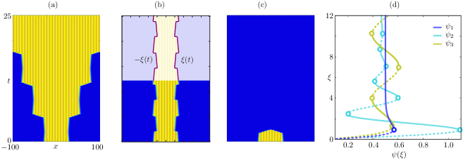
The interfacial description Coombes et al. (2012) applies in the case $f(u)=\Theta(u)$, where $\Theta(u)$ is the Heaviside step function. As customary, we consider localized regions of activity $-\xi(t)\leq x\leq\xi(t)$, where the interfaces (or threshold crossings) $x=\pm\xi(t)$ are defined by the level set conditions $u(\pm\xi(t),t)=h(t)$ with $\partial_{x}u(\pm\xi(t),t)\lessgtr 0$, for all $t\in\mathbb{R}^{+}$, and take their width $2\xi(t)$ as a measure of the spatial extent of the solution (see for instance Fig. 1(b)). Integrating (1), we find that solutions $u(x,t)$ can be expressed in terms of the interfacial functions $\xi(t)$ and the initial datum $u(x,0)$,

$$u(x,t)=e^{-t}u(x,0)+\int_{0}^{t}\int_{-\xi(s)}^{\xi(s)}e^{s-t}W(x,y)\,dy\,ds.$$ (2)

The approach of Refs. Coombes and Laing (2011); Coombes et al. (2012) can be extended to the case of time-dependent $h$. In this case differentiation of the level set condition for $\xi$ with respect to time leads to a closed scalar evolution equation for the half-width of the pattern. Using (1) we obtain

$$\varphi(\xi,t)\dot{\xi}=h+\dot{h}-\psi(\xi),$$ (3)

where $\varphi(\xi,t)=\partial_{x}u(\xi,t)$ and $\psi(\xi)=\int_{-\xi}^{\xi}W(\xi,y)\,dy$. By hypothesis $\varphi$ is strictly negative at all times. The function $\psi$ encodes the neural connectivity of the model, as it depends solely on the synaptic kernel $W$, which models arbitrary heterogeneous synaptic circuits. Figure 1(d) shows $\psi(\xi)$ for several commonly used kernels $W(\xi,y)$ and highlights that $\psi$ generically possesses folds. These are marked by circles in Fig. 1(d) and correspond to locations where $\psi^{\prime}=0$. Equation (3) represents an exact reduction of the field equation (1) for $u$ with a time-dependent threshold and Heaviside firing rate, and constitutes a key tool for the study of spatio-temporal canards.

If $h$ is a constant control parameter, Eq. (3) admits equilibria for all $h$ and $\xi$ such that $h=\psi(\xi)$. In other words, the curves in Fig. 1(d) can be interpreted as branches of steady (patterned) states of the full system (1) with the parameter $h$ identified with $\psi(\xi)$ in Fig. 1(d). This strategy for constructing patterns, contained in the original work of Amari Amari (1977), can be extended also to study stability: to each fold of $\psi$ corresponds a saddle-node bifurcation of the full system. In Ref. Avitabile and Schmidt (2015) it was shown that sinusoidal modulation of the kernel in space generates an infinite number of saddle-nodes organized in a snakes-and-ladders bifurcation structure Knobloch (2015).

The firing rate threshold parameter, $h$, is therefore a common continuation parameter in neural field studies: as $h$ is varied, we obtain branches of patterned stationary states and, depending on the choice of the kernel, secondary symmetry-breaking bifurcations may occur. It is therefore natural to search for canards in cases where $h$ is slowly varying. Variations of $h$ have been considered before in the literature: in Ref. Brackley and Turner (2007); Thul et al. (2016), the firing threshold was subject to fluctuations induced by noise, decoupled from the network activity; in Refs. Coombes and Owen (2005, 2007) the threshold $h$ was coupled directly to the local value of $u$, in order to mimic spike-frequency adaptation, observed experimentally in in vitro experiments of rat pyramidal neurons Madison and Nicoll (1984).

In the following we study spatio-temporal canards by combining a spatially-extended neural field with a slowly-varying oscillatory threshold $h(t)$ which may arise, for instance, from the competition between adaptation and facilitation processes, coupled to the neural field via the macroscopic width of the pattern, and describe a simple example of the dynamics that result when $h$ evolves on a slow time scale. Depending on the choice of control parameters, we consider limits where $h$ influences $u$ (but not vice-versa), as well as cases where the dynamics of $h$ and $u$ are fully coupled, as previously done in Refs. Brackley and Turner (2007); Thul et al. (2016) and Coombes and Owen (2005, 2007), respectively. Specifically, we study the extended neural field model

$$\partial_{t}u(x,t)=-u(x,t)+\!\!\int_{\mathbb{R}}W(x,y)\Theta\big{[}u(y,t)\!-\!h(t)\!\big{]}dy,$$ (4)

$$\ddot{h}(t)+\varepsilon^{2}h(t)=\varepsilon^{2}(\alpha+\beta\xi(t))+\varepsilon\gamma\dot{\xi}(t),$$

$$\xi(t)=\frac{1}{2}\int_{\mathbb{R}}\Theta\big{[}u(y,t)-h(t)\big{]}\,dy.$$

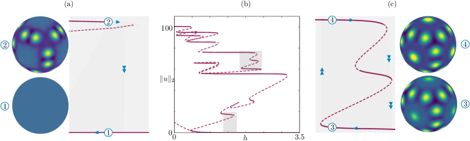
Thus $h$ obeys a weakly forced oscillator equation with a low natural frequency $\varepsilon$ that is coupled to the neural field via both $\xi$ and $\dot{\xi}$. In Figs. 1(a)–(c) we show direct simulations of the model (4), displaying strong sensitivity to changes in the parameter $\alpha$. We will show below that spatio-temporal canards organise abrupt transitions between branches patterned states, and are therefore responsible for the behavior shown in Figs. 1(a)–(c).

Interactions between excitable systems and slow oscillations are known to produce canard-type dynamics in ODEs with folded saddles Mitry et al. (2013); Desroches et al. (2016). This type of interaction motivated our choice of the coupling in model (4), which indeed produces canards in a spatially-extended system. In terms of the slow time $\tau=\varepsilon t$, system (4) is equivalent to

$$\varepsilon|\varphi_{\varepsilon}(\xi,\tau)|\dot{\xi} =\psi(\xi)-h-\varepsilon(q+\gamma\xi),$$ (5)

$$\dot{h} =q+\gamma\xi,$$

$$\dot{q} =\alpha+\beta\xi-h,$$

where $\varphi_{\varepsilon}$ is a rescaled version of $\varphi$ and we used the fact that $\varphi$ and $\varphi_{\varepsilon}$ are both strictly negative at all times. Crucially, we passed from model (4), which involves an evolution equation for the scalar field $u(x,t)$, to model (5), whose state variables are the scalars $(\xi(t),h(t))$. Since $\lim_{\varepsilon\to 0^{+}}\varepsilon|\varphi_{\varepsilon}(\xi,\tau)|=0$ for all $\tau\in\mathbb{R}^{+}$, Eqs. (5) take the form of a singularly perturbed system, with one fast variable $\xi$ and two slow variables $h$ and $q$. An important object for understanding the dynamics of such systems is the critical manifold $S^{0}$, defined as the $\varepsilon=0$ limit of the fast nullsurface Krupa and Szmolyan (2001). In the present case, this manifold is the folded surface $\{(h,q,\xi)\in\mathbb{R}^{3}\colon h=\psi(\xi)\}$. The limit yields the differential-algebraic system

$$0 =\psi(\xi)-h,$$ (6)

$$\dot{h} =q+\gamma\xi,$$

$$\dot{q} =\alpha+\beta\xi-h,$$

or equivalently the reduced system (or slow subsystem)

$$-\psi^{\prime}(\xi)\dot{\xi} =-q-\gamma\xi,$$ (7)

$$\dot{q} =\alpha+\beta\xi-\psi(\xi).$$

This system is singular when $\psi^{\prime}(\xi)=0$, that is, at the folds of the critical manifold separating attracting sheets from repelling ones. For the problem under consideration, the singularity occurs at fold lines $\{(h,q,\xi_{*})\in\mathbb{R}^{3}\colon h=\psi(\xi_{*}),\;\psi^{\prime}(\xi_{*})=0\}$; in passing we note that $\xi_{*}$ can be any of the folds marked by circles in Fig. 1(d). It is possible to remove this singularity by rescaling time by the factor $-\psi^{\prime}(\xi)$, leading to the desingularised reduced system (DRS)

$$\dot{\xi} =-q-\gamma\xi,$$ (8)

$$\dot{q} =\psi^{\prime}(\xi)\big{[}\psi(\xi)-\alpha-\beta\xi\big{]}.$$

We carry out this rescaling because it is helpful in deciphering the flow of system (7) near the fold lines. Indeed, the rescaling has two major consequences: (i) Orbits of system (7) are extended in system (8) to the fold lines, where (7) is undefined; (ii) System (7) may possess equilibria on the fold lines. As we shall see below, these equilibria are related to canards in system (8).

Figure 2: Examples of solutions containing spatio-temporal canards of folded-saddle type. (a): Time simulation of the folded-saddle case for $\alpha=0.5$, $\beta=\gamma=0$, and remaining parameters as in Fig. 1(b). (b): Solution to the full spatio-temporal model (4), also shown in (a) and in Fig. 1(b), projected on the $(h,q,\xi)$ phase space (blue), where we also plot the critical manifold $S^{0}$ (grey) and singular canards of (7) on $S^{0}$ (red). (c): Projection on the $(q,\xi)$ plane, showing the attracting (A) and repelling (R) sheets of $S^{0}$, revealing a spatio-temporal canard.

III Folded singularities and canards in the extended system

System (8) has an equilibrium at $(\xi_{*},-\gamma\xi_{*})$, where $\xi_{*}$ satisfies $\psi^{\prime}(\xi_{*})=0$, i.e., on a fold line of the surface $S^{0}$. This is not an equilibrium of the reduced system (7) because of the time rescaling by $-\psi^{\prime}(\xi)$, which reverses the orientation of trajectories on the repelling sheets of $S^{0}$. Therefore solutions to the reduced system (7) approach the point $(\xi_{*},-\gamma\xi_{*})$ along an attracting sheet of $S^{0}$, cross it in finite time, and continue to flow along a repelling sheet of $S^{0}$: these solutions of system (7) are called singular canards and persist for small $\varepsilon>0$ as canard solutions of system (5), and hence as spatio-temporal canards of system (4).

Equilibria $(\xi_{*},-\gamma\xi_{*})$ of the DRS (8) are called folded singularities (of node, saddle or focus type) and are therefore important in the classification of canards. Other equilibria of the DRS may exist as true equilibria of the reduced system (7): these states are not generically related to canards and are not considered here. The Jacobian at $(\xi_{*},-\gamma\xi_{*})$ is given by

$$\begin{pmatrix}-\gamma&-1\\ \pi(\xi_{*})&0\end{pmatrix},\qquad\pi(\xi_{*})=\psi^{\prime\prime}(\xi_{*})\big{[}\psi(\xi_{*})-\alpha-\beta\xi_{*}\big{]},$$

and hence $(\xi_{*},-\gamma\xi_{*})$ is either (i) a folded saddle (if $\pi(\xi_{*})<0$) or (ii) a folded node (if $0<\pi(\xi_{*})<\gamma^{2}/4$), corresponding in (5) to (i) excitable dynamics and (ii) mixed-mode dynamics.

Classical theory Desroches et al. (2012) now guarantees the presence of canards in (5), and these correspond to spatio-temporal canards in (4) for sufficiently small $\varepsilon>0$, close to the above-mentioned folded singularities.

Figure 3: Additional features of the folded-saddle scenario. In (a)–(b) we repeat the simulation of Fig. 2 with $\varepsilon=3.6\cdot 10^{-3}$, finding a periodic solution displaying a jump-on canard. (a): Projection of the trajectory of the full spatio-temporal model on the $(h,q,\xi)$ space (blue), where we also plot the critical manifold $S^{0}$ (grey) and singular canards on $S^{0}$ (red). (b): Projection on the $(q,\xi)$ plane with attracting (A) and repelling (R) sheets of $S^{0}$. In (c)–(d) we show a family of orbit segments passing near the folded saddle and displaying sensitivity to initial conditions, separating orbits jumping up towards (A) or jumping down towards another attracting sheet of $S^{0}$ (also marked as (A) in panel (b)).

We have confirmed these predictions using the full model (4) with the heterogeneous synaptic kernel

$$W(x,y)=\frac{1}{2}e^{-|x-y|}\Big{(}a+b\cos\frac{y}{\Lambda}\Big{)},$$ (9)

where $a,b\geq 0$, $\Lambda>0$ and the firing rate function

$$f(u)=(1+e^{-\mu u})^{-1}.$$ (10)

For $\mu\gg 1$ this sigmoidal function approximates a Heaviside firing rate employed in the theory. We use the spectral algorithm developed in Ref. Rankin et al. (2014) to solve the resulting equations. System (1), where $h$ is a fixed parameter, admits branches of localized steady states arranged in a characteristic snakes-and-ladders bifurcation structure exhibiting countably many folds at which $\psi^{\prime}(\xi_{*})=0$ (Fig. 1(d)).

III.1 Spatio-temporal folded-saddle canards

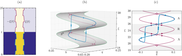
We first consider the uncoupled case with $\alpha=0.5$, $\beta=\gamma=0$, which leads to spatio-temporal folded-saddle canards. Figure 2(a) shows the solution of the full spatial system (4) in the form of a space-time plot while Fig. 2(b) shows the same results but projected onto the $(h,q,\xi)$ space (blue curve), compared with the singular canards of (7) (red curves). For reference we plot $S^{0}$ in grey. In Fig. 2(c) we show a projection onto the $(\xi,q)$ plane, where we indicate folded saddles (open circles) and the attracting (A) and repelling (R) sheets of $S^{0}$. For these parameters the theory predicts the presence of a folded-saddle spatio-temporal canard in system (4) and the projection indeed displays behavior typical of folded-saddle singularities in ODEs: the orbit follows the upper attracting sheet, passes the folded singularity from right to left (Fig. 2(c)) and then continues near a repelling sheet of $S^{0}$ for an $O(1)$ time, before a fast (anterior) jump leads to the lower attracting sheet; the orbit returns to the upper attracting sheet with a second (posterior) fast jump.

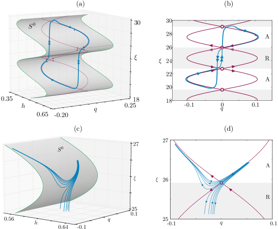
Since the latter jump occurs near a folded saddle, this opens the possibility of a jump-on canard segment, in which the orbit jumps and lands on the upper repelling sheet of $S^{0}$ before returning to the upper attracting one. We observe this behavior in canard cycles obtained with slightly different parameter values, as reported in Figs. 3(a)–(b): the solution is periodic and passes near four different folded-saddle singularities, marked with red circles in Fig. 3(b); this trajectory contains one clear canard segment near the topmost folded saddle; this segment is a jump-on canard, as the orbit makes a fast upward jump and then follows directly a repelling segment along the maximal canard of the folded saddle. The trajectory then passes near the other folded saddles, without displaying a clear canard segment.

In Figs. 3(c)–(d) we present a family of solutions of Eqs. (4) for different initial conditions near an attracting sheet of $S^{0}$. This experiment explains the sensitivity documented in Figs. 1(a)–(c), and highlights the transition through the canard in the folded-saddle case. This corresponds—modulo a change of direction near the repelling sheets of $S^{0}$—to a perturbation of the stable manifold of the folded saddle (as a saddle equilibrium of the DRS). Indeed, trajectories approach the canard and follow it past the folded saddle; the trajectories are then repelled and jump to a lower or upper attracting sheet of $S^{0}$, depending on their initial condition. In Fig. 3(d) we plot the singular canards associated with this folded saddle: the true canard (from A to R) and the so-called “false” (or faux) canard (from R to A), both shown in red. In this scenario, the true canard plays the role of a separatrix between trajectories that jump upwards, following the faux canard, and downwards, towards a different attracting sheet of $S^{0}$.

III.2 Spatio-temporal folded-node canards

Figure 4: Examples of solutions containing spatio-temporal canards of folded-node type. Parameters are as in Fig. 2, except $\alpha=\gamma=1$, $\beta=0$, for which the theory predicts folded-node canards. In (a)–(c) we plot the full spatio-temporal solution (a), its projection on the $(h,q,\xi)$ space (b) and on the $(q,\xi)$ plane (c); the latter show oscillations typical of folded-node canards, and therefore correspond to spatio-temporal folded-node canards in the neural field model. In (d)–(i) we set $\varepsilon=3.6\cdot 10^{-3}$, $\alpha=1$, $\gamma=0.7$ and retain all other parameter values; when initial conditions are varied slightly, a variable number of small oscillations is found near the folded node, as expected from the ODE theory. We set $q(0)=-18.35$ (label 1 in (d), (e), (f), (i)) and $q(0)=-18.40$ (label 2 in (f), (g), (h), (i)). (f): Projections on the $(q,\xi)$ plane, revealing an initial drift near the folded node, during which trajectory 1 (2) displays 3 (5) small-amplitude oscillations around the folded singularity (see inset (i)).

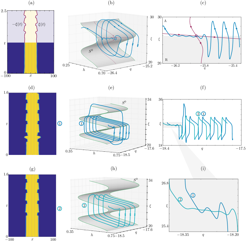
We next repeat our numerical analysis for the fully coupled system (4) when $\alpha=1$, $\beta=0$, $\gamma=1$ for which the theory predicts spatio-temporal canards of folded-node type (Fig. 4(a)–(c)). The folded-node scenario is richer than the folded-saddle one: first, solutions containing canard segments exist for $O(1)$ ranges of initial conditions and parameter values; second, there are many more possible waveforms due to the existence of a funnel region around the folded-node singularity that induces a rotation of the trajectories as they pass through it; this effect is clearly visible in Fig. 4(b)–(c) as small amplitude spiraling motion in the vicinity of the fold, and rather less clearly as the minute oscillations for $t\in[0,1.5]$ in Fig. 4(a). As initial conditions change, the number of these small (subthreshold) oscillations in the funnel region varies and this phenomenon defines rotation sectors near $S^{0}$. The boundaries between different rotation sectors correspond to canard solutions generating mixed-mode dynamics in the system. For fixed parameter values, the maximum number of subthreshold oscillations is given by the eigenvalue ratio of the folded node Desroches et al. (2012), seen as an equilibrium of Eqs. (8). Thus trajectories with different initial conditions will be trapped in the funnel and pass near the folded node while making different numbers of subthreshold oscillations, thereby encoding the possible waveforms in this regime.

We exemplify this behavior in Figs. 4(d)–(i) by time-stepping (4) with slightly different initial conditions, close to a folded node, when $\alpha=1$, $\beta=0$, $\gamma=0.7$. In the experiment under consideration we pre-computed a stationary pattern $u_{0}(x)$ for the neural field equation with constant firing rate threshold, $h=0.57$, $\dot{h}=0$, that is, we select a stationary state on $S^{0}$. We then perturb this state and compute two trajectories, with initial conditions close to the folded node by setting $u(x,0)=u_{0}(x)$, $h(0)=0.58$, $q(0)=-18.40$ (label 1) and $q(0)=-18.35$ (label 2). Figures 4(d,g) show the corresponding space-time evolution $u(x,t)$ while Figs. 4(e,h) show the corresponding trajectories in $(h,q,\xi)$ space. Panel (c) and the enlargement in (f) show the projections of these trajectories on the $(q,\xi)$ plane. The trajectories are initially close and exhibit the drifting and spiralling motion predicted by the theory Desroches et al. (2012), with respectively three and five subthreshold oscillations near the folded node. After an initial transient, in which trajectory 1 visits the upper attracting sheet of $S^{0}$, both trajectories wrap clockwise around the middle and bottom attracting sheets of $S^{0}$ (Figs. 4(e,h)). Both also display jump-on canard segments at every turn, in the vicinity of the left boundary of the upper repelling sheet of $S^{0}$, although these become less pronounced as time increases.

IV Neural fields posed on a sphere

We have also studied neural field models posed on a more realistic spherical domain and identified spatio-temporal canards with octahedral symmetry where interfaces are no longer points but curves in 3D. The above theory does not readily generalize to this setting but we nevertheless successfully tested its predictions in the folded-saddle case, when $u$ and $h$ are decoupled. As shown in Fig. 5, the model displays orbits with canard segments (and canard cycles). In this case the system with constant $h$ admits an intricate bifurcation diagram (not shown), where coexisting stable states with octahedral, icosahedral and rotational symmetry are interconnected via symmetry-breaking bifurcations and saddle-node bifurcations.

Figure 5: Spatio-temporal canards of folded-saddle type occurring in a neural field model posed on a spherical domain using $h$ as the continuation parameter. (b) Bifurcation diagram of steady states with octahedral symmetry in the system (11). (a,c) Bifurcation diagram (red), orbit (blue) and representative patterns obtained when $h$ varies slowly through (a) a low-lying fold, and (c) one of the higher folds. When the evolution of $h$ is decoupled from $u$, we observe spatio-temporal canards of folded-saddle type (see the animations canardCycle.mp4, canardDown.mp4, canardUp.mp4 for further details).

The calculations for neural fields posed on the unit sphere were performed using a neural field model with a constant threshold crossing $h$,

$$\partial_{t}u(\bm{x},t) =-u(\bm{x},t)$$ (11)

$$+\kappa\int_{\mathbb{S}^{2}}W\big{(}\langle\bm{x},\bm{y}\rangle\big{)}f\big{(}u(\bm{y},t)-h\big{)}\,d\sigma(\bm{y}),$$

where $\bm{x}\in\mathbb{S}^{2}=\{\bm{z}\in\mathbb{R}^{3}\colon|\bm{z}|=1\}$ and the integral is over $\mathbb{S}^{2}$. In this integro-differential equation the kernel $W$ models the synaptic wiring between two points $\bm{x},\bm{y}$ on the surface of a sphere; we assume that this wiring depends solely on the great-circle distance (geodesic) between $\bm{x}$ and $\bm{y}$, hence the dependence on the scalar product $\langle\bm{x},\bm{y}\rangle$. We use an excitatory-inhibitory Gaussian synaptic kernel

$$W(\xi)=A_{1}\exp(-\xi^{2}/B_{1})-A_{2}\exp(-\xi^{2}/B_{2}).$$ (12)

Stationary patterned states of (11) were continued in the parameter $h$ using a Nyström scheme, combined with standard path-following techniques as well as high-order, highly efficient, icosahedral- or tetrahedral-invariant quadrature schemes. A comprehensive study of branches of patterned states supported by this model, their symmetries and stability, as well as the properties of the numerical scheme will be described in a separate publication Avitabile et al. (2017). A sample result showing a branch of states with octahedral symmetry is reported in Fig. 5(b). Solutions with this symmetry bifurcate transcritically from the homogeneous steady state, and then undergo a sequence of saddle-nodes and symmetry-breaking bifurcations shown in the figure.

We are interested in testing the predictions of the theory developed for 1D domains for more realistic cortical surfaces. For physical domains in higher dimensions, it is possible to reduce the equations as for 1D domains, but the reduction is still a spatially-extended dynamical system. In 1D, the activity set is given by $\mathcal{A}(t)=[-\xi(t),\xi(t)]\in\mathbb{R}$ and, differentiating one of the threshold conditions, say $u(\xi(t),t)=h(t)$, we obtain

$$\partial_{x}u(\xi(t),t)\dot{\xi}(t)=h(t)+\dot{h}(t)-\int_{-\xi(t)}^{\xi(t)}W(x,y)\,dy$$ (13)

which is an evolution equation for the scalar variable $\xi$. To extend this procedure to the sphere, we assume that the activity set $\mathcal{A}(t)=\{\bm{x}\in\mathbb{S}^{2}\colon u(\bm{x},t)\geq h(t)\}$ has a boundary which can be parameterized as follows,

$$\partial\mathcal{A}(t) =\bigcup_{k=1}^{K}\mathcal{C}_{k}(t),$$

$$\mathcal{C}_{k}(t) =\{\bm{x}\in\mathbb{S}^{2}\colon\bm{x}=\bm{\xi}_{k}(s,t),\;s\in[0,2\pi)\},$$

where the functions $\{\bm{\xi}_{k}\}$ are $2\pi$-periodic and smooth in the variable $s$. In other words, we assume that the boundary of the activity set on the spherical domain is the union of $K$ disjoint curves on the spherical surface $\mathbb{S}^{2}$. We seek evolution equations for the functions $\{\bm{\xi}_{k}\}$. Since the solution $u(\bm{x},t)$ crosses the threshold $h(t)$ on each of the curves $\mathcal{C}_{k}$, we differentiate the threshold condition $u(\bm{\xi}_{k}(s,t),t)=h(t)$ with respect to $t$ to obtain

$$\big{\langle}\bm{\nabla}u\big{(}\bm{\xi}_{k}(s,t),t\big{)}, \;\partial_{t}\bm{\xi}_{k}(s,t)\big{\rangle}=h(t)+\dot{h}(t)$$ (14)

$$-\int_{\mathcal{A}(t)}W\big{(}\langle\bm{\xi}_{k}(s,t),\bm{y}\rangle\big{)}\,d\sigma(\bm{y}),$$

$$s\in[0,2\pi),\quad k=1,\ldots,K,$$

$$\bm{\xi}_{k}(0,t) =\bm{\xi}_{k}(2\pi,t),\quad k=1,\ldots,K,$$ (15)

where the gradient is in spherical coordinates. It can be shown that, under suitable assumptions on the kernel, the inner product on the left hand side and the surface integral on the right hand side of (14) can be written Coombes et al. (2012, 2013) in terms of line integrals over the closed curves $\mathcal{C}_{k}(t)$. The system (14)–(15) is therefore closed and represents a generalization of (13). In this case, however, the state variables are the functions $\{\bm{\xi}_{k}(s)\}$, as opposed to the scalar $\xi$, and a canard theory for this system is currently unavailable.

We can, however, simulate the system (11) or the system (14)–(15) numerically and search for evidence of spatio-temporal canards. More precisely, we have performed numerical experiments to test the robustness of the 1D theory to

1. Changes in the geometry of the problem: the spherical model includes curvature effects via the great-circle distance $\langle\bm{x},\bm{y}\rangle$ between points $\bm{x}$, $\bm{y}$ on the spherical cortex (see Eq. (11)).

2. Changes in the synaptic connectivity function: the kernel (12) is different from that used in the 1D computations; in particular, the kernel (12) is excitatory-inhibitory and homogeneous while kernel (9) is purely excitatory and heterogeneous.

3. Changes in the firing rate function: the theory is valid for a Heaviside firing rate which is approximated in the 1D simulations by a steep sigmoid (Eq. (10) with $\mu=50$); in the spherical simulations we employ a shallow firing rate ($\mu=8$).

4. Changes in the evolution equation of the firing threshold $h$: in the spherical simulations, $h$ evolves slowly and independently from $u$, but not harmonically:

   $$h(t)=\begin{cases}\varepsilon t+h_{0}&0\leq t<(h_{1}-h_{0})/\varepsilon\\ -\varepsilon t+2h_{1}-h_{0}&t\geq(h_{1}-h_{0})/\varepsilon,\end{cases}$$ (16)

   where $h_{1}$ is a fold point in the bifurcation diagram (located using standard bifurcation analysis techniques) and $h_{0}<h_{1}$. Consequently, $h$ undergoes a slow linear increase up to the fold, followed by a slow linear decrease.

In each case we found that the qualitative predictions of the 1D theory carried over to this much more complicated situation.

V Conclusions and perspectives

To the best of our knowledge, this article presents the first theory for folded-singularity temporal canards in a spatially-extended system. This result paves the way towards a systematic study of spatio-temporal mixed-mode oscillations (MMOs) in spatially-extended systems, with the view of explaining the origin of MMOs observed in spatio-temporal signals modelling spike-frequency adaptation and synaptic depression Folias and Bressloff (2005b). The spatio-temporal structures discussed here are also directly relevant to neural mass and connectomic models, in which a discrete connectomic matrix replaces the heterogeneous kernel $W$ Haimovici et al. (2013): canard structures in these models would offer a rigorous explanation of the brutal transitions observed, for instance, in models of partial epilepsy Proix et al. (2014). There is a general consensus that spike (and more generally burst) timings, durations and rates are involved in information coding in the brain Borst and Theunissen (1999). Being able to identify boundaries (represented by spatio-temporal canards) between different activity regimes (e.g. spiking/bursting or mixed-mode oscillations with different signatures) may shed further light on the transmission of information in the brain.
Acknowledgement: This work was supported in part by the Engineering and Physical Sciences Research Council under grant EP/P510993/1 (DA) and by the National Science Foundation under grant DMS-1613132 (EK). DA thanks Luke Wood and Oliver Smith for their work on neural field models during their final-year undergraduate dissertations.

Author contributions: DA and MD contributed equally to this work.

References

- Bressloff (2012) P. C. Bressloff, J. Phys. A 45, 033001 (2012).
- Bressloff (2014) P. C. Bressloff, Waves in Neural Media (Springer, New York, NY, 2014).
- Ermentrout and Terman (2010) G. B. Ermentrout and D. H. Terman, Mathematical Foundations of Neuroscience (Springer, New York, 2010).
- Wilson and Cowan (1972) H. R. Wilson and J. D. Cowan, Biophys. J. 12, 1 (1972).
- Amari (1975) S.-I. Amari, Biol. Cybern. 17, 211 (1975).
- Folias and Bressloff (2005a) S. Folias and P. Bressloff, Phys. Rev. Lett. 95, 208107 (2005a).
- Richardson et al. (2005) K. A. Richardson, S. J. Schiff, and B. J. Gluckman, Phys. Rev. Lett. 94, 028103 (2005).
- Huang et al. (2004) X. Huang, W. C. Troy, Q. Yang, H. Ma, C. R. Laing, S. J. Schiff, and J.-Y. Wu, J. Neurosci. 24, 9897 (2004).
- González-Ramírez et al. (2015) L. R. González-Ramírez, O. J. Ahmed, S. S. Cash, C. E. Wayne, and M. A. Kramer, PLoS Comput. Biol. 11, e1004065 (2015).
- Steyn-Ross et al. (2003) M. L. Steyn-Ross, D. A. Steyn-Ross, J. W. Sleigh, and D. R. Whiting, Phys. Rev. E 68, 021902 (2003).
- Camperi and Wang (1998) M. Camperi and X.-J. Wang, J. Comput. Neurosci. 5, 383 (1998).
- Benoît et al. (1981) E. Benoît, J.-L. Callot, F. Diener, and M. Diener, Collect. Math. 32, 37 (1981).
- Krupa and Szmolyan (2001) M. Krupa and P. Szmolyan, J. Differ. Equations 174, 312 (2001).
- Desroches et al. (2013a) M. Desroches, M. Krupa, and S. Rodrigues, J. Math. Biol. 67, 989 (2013a).
- Mitry et al. (2013) J. Mitry, M. McCarthy, N. Kopell, and M. Wechselberger, J. Math. Neurosci. 3, 1 (2013).
- Moehlis (2006) J. Moehlis, J. Math. Biol. 52, 141 (2006).
- Kramer et al. (2008) M. A. Kramer, R. D. Traub, and N. J. Kopell, Phys. Rev. Lett. 101, 68103 (2008).
- Rinzel (1987) J. Rinzel, in Proc. Intern. Congr. Math., Vol. 1-2 (Amer. Math. Soc., Providence, RI, 1987) pp. 1578–1593.
- Desroches et al. (2012) M. Desroches, J. Guckenheimer, B. Krauskopf, C. Kuehn, H. M. Osinga, and M. Wechselberger, SIAM Rev. 54, 211 (2012).
- Desroches et al. (2013b) M. Desroches, T. J. Kaper, and M. Krupa, Chaos 23, 046106 (2013b).
- Gandhi et al. (2016) P. Gandhi, C. Beaume, and E. Knobloch, in Nonlinear Dynamics: Materials, Theory and Experiments, edited by M. Tlidi and M. G. Clerc (Springer, New York, 2016) pp. 303–316.
- Coombes (2005) S. Coombes, Biol. Cyber. 93, 91 (2005).
- Laing and Troy (2003) C. R. Laing and W. C. Troy, SIAM J. Appl. Dyn. Sys. 2, 487 (2003).
- Rankin et al. (2014) J. Rankin, D. Avitabile, J. Baladron, G. Faye, and D. J. B. Lloyd, SIAM J. Sci. Comput. 36, B70 (2014).
- Bressloff (2001) P. C. Bressloff, Phys. D 155, 83 (2001).
- Coombes and Laing (2011) S. Coombes and C. Laing, Phys. Rev. E 83, 011912 (2011).
- Avitabile and Schmidt (2015) D. Avitabile and H. Schmidt, Phys. D 294, 24 (2015).
- Laing et al. (2002) C. R. Laing, W. C. Troy, B. Gutkin, and G. B. Ermentrout, SIAM J. Appl. Math. 63, 62 (2002).
- Coombes et al. (2003) S. Coombes, G. Lord, and M. Owen, Phys. D 178, 219 (2003).
- Coombes et al. (2012) S. Coombes, H. Schmidt, and I. Bojak, J. Math. Neurosci. 2, 9 (2012).
- Amari (1977) S.-I. Amari, Biol. Cybern. 27, 77 (1977).
- Knobloch (2015) E. Knobloch, Annu. Rev. Condens. Matter Phys. 6, 325 (2015).
- Brackley and Turner (2007) C. A. Brackley and M. S. Turner, Phys. Rev. E 75, 041913 (2007).
- Thul et al. (2016) R. Thul, S. Coombes, and C. R. Laing, J. Math. Neurosci. 6, 1 (2016).
- Coombes and Owen (2005) S. Coombes and M. R. Owen, Phys. Rev. Lett. 94, 148102 (2005).
- Coombes and Owen (2007) S. Coombes and M. R. Owen, in Fluids and Waves: Recent Trends in Applied Analysis: Research Conference, May 11-13, 2006, the Universtiy of Memphis, Memphis, TN, Vol. 440 (American Mathematical Soc., 2007) p. 123.
- Madison and Nicoll (1984) D. V. Madison and R. A. Nicoll, J. Physiol. 354, 319 (1984).
- Desroches et al. (2016) M. Desroches, M. Krupa, and S. Rodrigues, Phys. D 331, 58 (2016).
- Avitabile et al. (2017) D. Avitabile, R. Nicks, and O. Smith, in preparation (2017).
- Coombes et al. (2013) S. Coombes, H. Schmidt, and D. Avitabile, in Neural Field Theory, edited by S. Coombes, P. beim Graben, R. Potthast, and J. J. Wright (Springer, New York, 2013) pp. 187–211.
- Folias and Bressloff (2005b) S. E. Folias and P. C. Bressloff, SIAM J. Appl. Math. 65, 2067 (2005b).
- Haimovici et al. (2013) A. Haimovici, E. Tagliazucchi, P. Balenzuela, and D. R. Chialvo, Phys. Rev. Lett. 110, 178101 (2013).
- Proix et al. (2014) T. Proix, F. Bartolomei, P. Chauvel, C. Bernard, and V. K. Jirsa, J. Neurosci. 34, 15009 (2014).
- Borst and Theunissen (1999) A. Borst and F. E. Theunissen, Nat. Neurosci. 2, 947 (1999).