Effect of Scrape-Off-Layer Current on Reconstructed Tokamak Equilibrium

Abstract

Methods are described that extend fields from reconstructed equilibria to include scrape-off-layer current through extrapolated parametrized and experimental fits. The extrapolation includes both the effects of the toroidal-field and pressure gradients which produce scrape-off-layer current after recomputation of the Grad-Shafranov solution. To quantify the degree that inclusion of scrape-off-layer current modifies the equilibrium, the $\chi$-squared goodness-of-fit parameter is calculated for cases with and without scrape-off-layer current. The change in $\chi$-squared is found to be minor when scrape-off-layer current is included however flux surfaces are shifted by up to $3\;cm$. The impact on edge modes of these scrape-off-layer modifications is also found to be small and the importance of these methods to nonlinear computation is discussed. Published version: Phys. Plasmas 24, 012504 (2017) [http://dx.doi.org/10.1063/1.4972822]

I Introduction

Understanding of tokamak plasmas has greatly benefited from the separation of time scales inherent in strongly magnetized plasmas. All orderings of strongly-magnetized plasma equations show that the magnetic pressure and line-bending contributions from $\mathbf{J}\times\mathbf{B}$ and the force-density from $\nabla p$ are the largest terms in the center-of-mass momentum equation. Assuming symmetry and nested flux surfaces allows one to derive the Grad-Shafranov equation Shafranov (1971) that describes the lowest-order steady-state fields. This solution is conventionally described as the plasma equilibrium. Perturbations that drive the plasma away from equilibrium launch Alfvén waves that quickly act to restore the plasma to equilibrium Jenkins et al. (2010). Transport occurs on slower time scales, while symmetry-breaking macroscopic instabilities occur on intermediate time scales between the transport and the stiff Alfvén time scale.

This paradigm well-describes the experimental phenomenology, and solutions to the Grad-Shafranov equation are routinely calculated hundreds of times per plasma discharge to provide a measure of the location of magnetic-flux surfaces. As such, these solutions are indispensable to controlling the plasma and interpreting diagnostic data. Thus Grad-Shafranov theory may be considered as one of the most successful applications of tokamak-plasma theory. Measurement of both the macro- and micro-scopic perturbations confirms the small-fluctuation assumption embedded in the theory: tearing modes, for example, have perturbed magnetic energies four orders of magnitude below the equilibrium stored magnetic energy Sauter et al. (1997), and ion-temperature-gradient-driven turbulence produces density fluctuations less than one percent of the equilibrium density White et al. (2008). The small-fluctuation hierarchy coupled with slow temporal evolution permits the common approach of extended-MHD modeling about a Grad-Shafranov equilibrium (e.g. Ref. King et al. (2017)), as opposed to modeling the symmetric fields with the full extended-MHD equations (e.g. Ref. Ferraro and Jardin (2009)). The effects encompassed by extended-MHD are variable: extended-MHD refers to models beyond resistive MHD that include some combination of anisotropic thermal conduction and stresses Sovinec et al. (2004), two-fluid evolution Sovinec and King (2010), finite-Larmor-radius closures Schnack et al. (2006); King et al. (2011), and/or advanced drift-kinetic-equation closures Held et al. (2015).

One challenge to simulating small fluctuations about an equilibrium state is that errors in the equilibrium can be on the order of the perturbation magnitude. This issue is recognized by Grimm et al. Grimm et al. (1976) with the first ‘mapping code’, a code that employs numerical maps to transfer fields from the spatial discretization of an equilibrium code onto the spatial discretization of another code, where the second code typically assesses stability or the evolution of nonlinear perturbations. Despite considerable effort to increase the accuracy of mapping codes, mapping errors are difficult, if not impossible, to completely eliminate. In practice, extended-MHD codes, such as nimrod Sovinec et al. (2004); Sovinec and King (2010) and m3d-c1 Jardin et al. (2007); Ferraro et al. (2010), recompute the Grad-Shafranov equilibrium with their native spatial discretizations to circumvent these errors. Burke et al. Burke et al. (2010) discusses an example of the impact of mapping errors. In that work, the nimrod extended-MHD code is benchmarked with the linear-MHD codes gato Bernard et al. (1981) and elite Snyder et al. (2002) on peeling-ballooning modes in tokamak equilibria. gato, like other global linear-MHD codes, uses mapped equilibria while elite uses Miller equilibria Miller et al. (1998) that effectively act to provide the same accuracy as re-solving the Grad-Shafranov equation. In nimrod calculations with mapped equilibria, better agreement with gato is obtained, whereas when the nimeq code Howell and Sovinec (2014) is used to recompute the Grad-Shafranov equation for the nimrod initial condition, better agreement with elite is obtained.

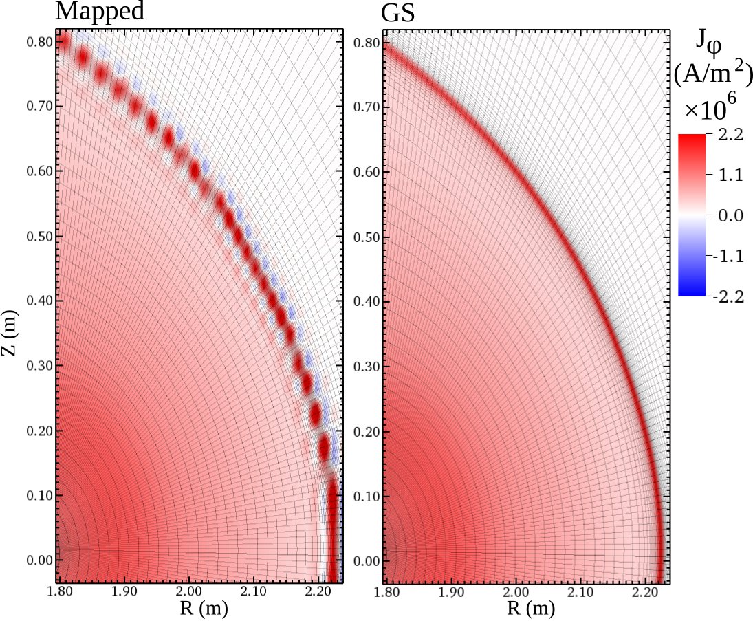
Figure 1: [color online] Toroidal current on the upper half of the outboard midplance from equilibria that are mapped (left) and that use a recomputed Grad-Shafranov solution (right). From a reconstruction of DIII-D shot 145098 at 1800 ms.

While this example demonstrates the importance of high-accuracy Grad-Shafranov solutions that are recomputed within a code’s native spatial discretization, a further example is provided with Fig. 1. The figure shows a comparison of the toroidal current density from both a mapped equilibrium along with a case where the Grad-Shafranov solution is recomputed with nimeq. This high-resolution computation is performed with a $72\times 512$ finite-element grid with bi-quartic elements. The bumps in the mapped solution roughly correspond to the resolution of the $129\times 129$ grid used during the reconstruction. Computations of edge-mode growth rates with the mapped equilibria give markedly different results relative to using the solution recomputed with nimeq.

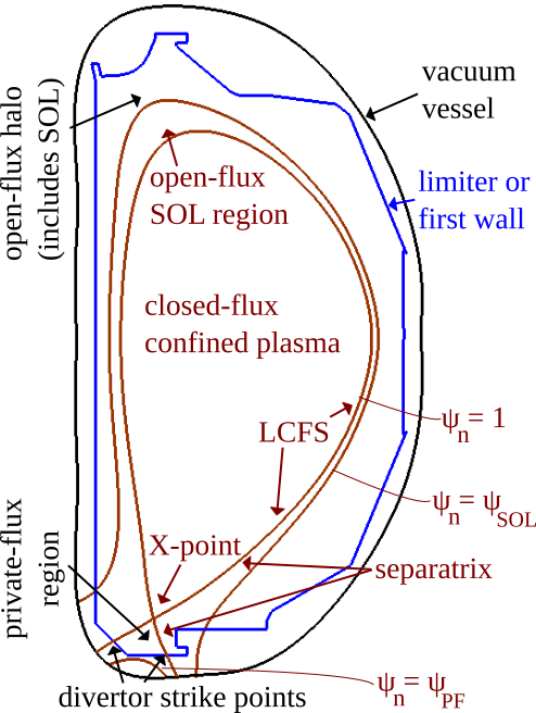
Figure 2: [color online] Diagram of topological regions of a diverted, lower-single-null shot within the DIII-D tokamak.

The work of Burke et al. considered the simple case of an artificial peeling-ballooning equilibrium with exclusively closed and nested-flux surfaces without diverted magnetic topology. A diagram of the topology associated with cases considered in this work, a diverted lower-single-null shot within the DIII-D tokamak, is shown in Fig. 2 along with labels of the terminology used for the topological regions and contours. Operation with a divertor implies the presence of a separatrix field line that separates the open- and closed-flux regions. The surface immediately inside the separatrix is the last-closed-flux surface (LCFS). The separatrix and LCFS are indistinguishable from a practical standpoint, aside from the separatrix field lines that extend to the divertor strike point. The open field lines between the LCFS and the first wall define the halo region Strauss et al. (2004); Kruger et al. (2005), and in the modeling of Burke et al. this region was approximated as a closed-field-line region. Traditionally in linear-MHD modeling, this halo region is treated as a vacuum; i.e., it has neither current nor plasma density. In extended-MHD modeling, the term halo region is used instead to denote that it is a cold-plasma region, capable of containing current, surrounding the hot, closed-field-line region.

The goal of this work is to relax the vacuum constraint of the halo region while remaining consistent with the measurements that are used to produce the reconstruction. For model fidelity to experiments, it is important to carefully consider the vacuum assumption in the halo region relative to the dynamics of study. Edge modeling is likely sensitive to current and flows present in the scrape-off-layer (SOL) region Groth et al. (2007), a subregion of the halo that directs the energy and particle exhaust from the hot plasma onto the divertor. Most published simulations to date are initialized from equilibrium that do not have current or flow in the halo region. This is largely because this current is typically not included in reconstructed equilibria from the highly successful, workhorse efit code Lao et al. (1985a, b). Without SOL current, reconstructions must have one of two undesirable properties: 1) either there is an artificial constraint on the current which must smoothly vanish at the separatrix or 2) there is a current discontinuity at the separatrix. The former constraint leads to the incorrect edge profiles, whereas the latter impacts convergence – particularly for high-order spatial discretizations such as those employed by nimrod and m3d-c1. Importantly, cases with either constraint fail to include the measured profiles outside the LCFS.

In this paper, we discuss our method for adding SOL current to equilibrium reconstructions generated by efit. One notable case that uses this method is the DIII-D QH-mode modeling in Ref. King et al. (2017). The difficulties with the current and flow discontinuities and a desire for more accurate modeling of the QH-mode instabilities motivated the development of our methods that include SOL profile gradients. This paper begins by reviewing details of the efit reconstructions, and discussing important metrics for determining the quality of the reconstructions in Sec. II. The methods for recomputing equilibria with separatrices along with the details on how we add SOL current to these new equilibria are described in Sec. III. Example cases that use these methods are introduced in Sec. IV. We then compare the new and original equilibria using synthetic diagnostics that are similar to those used to constrain the original reconstructed equilibrium in Sec. V. Finally, we examine the minor modification to the linear growth rates of peeling-ballooning modes (PBMs) by the addition of SOL current in Sec. VI before making concluding remarks in Sec. VII.

II Overview of efit equilibrium reconstructions

Determination of the experimental configuration of tokamak plasmas has become essential for understanding and optimizing stability and confinement in fusion research devices. Reconstruction of the experimental equilibrium from a combined set of magnetic, temperature and density measurements is computed by minimizing the error between modeled and observed signals. This technique, now routine, was pioneered with the efit code which originally used only magnetic diagnostics external to the first wall as a constraint Lao et al. (1985a, b). Later, the motional Stark effect diagnostic Wroblewski et al. (1990); Rice et al. (1999) greatly improved the accuracy of the reconstructions by providing internal measurements of the magnetic and electric fields. More recently, measurements of the density and temperature profiles via Thompson scattering Carlstrom et al. (1992); Eldon et al. (2012) and charge exchange recombination (CER) Groebner et al. (1990); Chrystal et al. (2015) spectroscopy provide further constraints on the pressure profiles Lao et al. (1990).

To quantify a reconstruction’s accuracy, results from efit Grad-Shafranov solves are applied to a $\chi$-squared test against the experimental measurements. In other words, the goal is to find a Grad-Shafranov solution that minimizes

$$\chi^{2}=\sum_{i}{\left(\frac{M_{i}-C_{i}}{\sigma_{i}}\right)^{2}}$$ (1)

where $M_{i}$ is the measured signal, $C_{i}$ is the computed signal, and $\sigma_{i}$ is the measurement uncertainty. In this paper, we perform this $\chi$-squared calculation to quantify the change that arises from the numerical errors associated with mapping, our recomputation of the Grad-Shafranov solution, and the addition of the SOL pressure profiles and associated current during the recomputation.

Typically, efit reconstructions do not include SOL current and treat the region between the separatrix and wall, i.e. the halo region, as current free. This implies that if the plasma discharge has a finite current on the separatrix, which is often the case for H-mode discharges that contain large bootstrap and Pfirsch-Schlüter currents, there will be a discontinuity at the LCFS. Equivalently within the context of the Grad-Shafranov equation, the efit profiles are constrained such that the pressure and toroidal magnetic field are constant in the halo region. With finite gradients at the LCFS, this leads to discontinuities in the first derivatives of these profiles. These inconsistencies lead to subtle but significant issues when evolving tokamak-edge unstable cases initialized from efit reconstructions. For example, in codes that retain the magneto-sonic wave physics both the SOL current and profile gradients must be included such that the equilibrium is consistent with force balance. Furthermore during nonlinear computations, any inconsistencies to the Grad-Shafranov equation, including discretization errors from discontinuous fields, can launch spurious magneto-sonic waves.

It must be noted that efit has the ability to include force-free, poloidal current in the SOL through finite gradients in the toroidal magnetic flux Lao and Jensen (1991); Strait et al. (1991). However, this capability is rarely exercised and there is no published work on the inclusion of finite pressure gradients in the SOL.

III Algorithms: Bounding Contours and SOL Fits

Initializing a nimrod computation from a reconstruction is a two-step process that involves mapping from the reconstructed equilibrium, and then recomputation of the equilibrium. The mapping code fluxgrid creates both a partially flux-aligned finite-element mesh and maps the reconstructed-equilibrium fields onto this mesh. This mapped solution is refined through solution of the Grad-Shafranov equation with the nimeq code Howell and Sovinec (2014). The solution can then be iteratively passed between fluxgrid and nimeq for further grid refinement and Grad-Shafranov solves, as needed. The Grad-Shafranov solve is formulated as a boundary-value problem where the boundary condition is specified by the value of $\psi$ from the mapped reconstruction. This boundary condition constrains both the fields from the external coils and those generated by the internal plasma that are also determined by the pressure and toroidal-flux profiles. With this method, the recomputed fields closely resemble the reconstructed versions; however, mapping errors are largely eliminated and the Grad-Shafranov equation is satisfied up to an input tolerance.

Relative to the methods described in Ref. Howell and Sovinec (2014), we employ extensions that identify the open- and closed-flux regions of the domain in order to apply the appropriate fitted form of the pressure and toroidal flux profiles. Within the closed-flux regions, these profiles are specified by efit reconstructions as a function of normalized flux ($\psi_{n}=(\psi-\psi_{o})/(\psi_{x}-\psi_{o})$ which is zero at the O-point where $\psi=\psi_{o}$ and unity on the separatrix where $\psi=\psi_{x}$). With the exception of private-flux regions, regions with $\psi_{n}<1$ contain closed field lines and regions with $\psi_{n}>1$ contain open-field lines. Applying these profiles to the domain requires identification of the closed-flux region. In practice, we find the bounding LCFS contour and use a simple algorithm that counts the number of crossings of a line that extends from a finite-element node to the boundary to determine if each node is enclosed by the contour. The separatrix contour and location of the extrema of $\psi$ in the core are allowed to change and must be recomputed after each iteration of the Grad-Shafranov solve. As the X-point on the separatrix contour associated with diverted magnetic topology consists of a stagnation point for field-line tracing, we instead elect to find a contour vanishingly close to the separatrix which numerically approximates the LCFS. For our purposes, we only need to bound the finite-element nodes that are within the separatrix. We employ two methods that use field-line tracing of the polodial field to find this approximate LCFS contour. The first method uses bisection of the domain to determine where the field lines transition from closed to open within a specified tolerance. For the parallel implementation, it becomes an N-section method where each core is assigned a seed point between the known closed- and open-field-line locations. The second method is to use the oculus code to find the saddle point in $\psi$ that is associated with the X-point, and a field-line seeded with a vanishingly small offset towards the O-point is used as the LCFS in order to avoid stagnation of the field-line tracing near the X-point. The latter method has the advantage of being somewhat more robust for high-resolution cases, but the disadvantage of not being amenable to a straight-forward parallel implementation.

As discussed earlier, efit solutions have zero profile gradients outside the LCFS. A cubic-spline fit of this data is used to evaluate these fields within the LCFS. Equilibrium generated using these spline fits with constant profile values outside the LCFS closely match the solution given by efit while largely eliminating mapping errors. One goal of this work is to contrast this recomputed solution with a solution that contains SOL-profile gradients.

SOL-profile gradients and associated currents are included by defining bounding contours and normalizing the flux as an extension to the methods used to determine the open- and closed-flux regions. The SOL region is defined as the region between the LCFS contour and contours with $\psi_{n}=\psi_{sol}$ and $\psi_{n}=\psi_{pf}$ where $\psi_{sol}$ ($>1$) defines a contour(s) at the edge of the SOL region and $\psi_{pf}$ ($<1$) defines a contour(s) in the private-flux region(s) (see Fig. 2). The algorithm that determines these contours is able to handle an arbitrary number of intersections of this region and the computational boundary of the domain and thus diverted topology such as double null configurations is tractable. The algorithm works as follows: The initial SOL bounding region is assumed to be the computational boundary. The algorithm checks the value of $\psi_{n}$ at each finite-element node location outside the LCFS but contained within this ‘working’ SOL region. If the condition $\psi_{pf}<\psi_{n}<\psi_{sol}$ is not satisfied, the location between the wall and the O-point where $\psi_{n}=\psi_{sol}$ or $\psi_{n}=\psi_{pf}$ is identified, and a new contour is traced. Absent integration error, the new contour is terminated at the boundary. The section of the domain that does not encircle the O-point is removed from the ‘working’ SOL region until only nodes with the property $\psi_{pf}<\psi_{n}<\psi_{sol}$ remain. This new SOL contour, in addition to the LCFS contour, bound the SOL region.

The appropriate pressure and toroidal magnetic flux profiles are defined within the SOL region via two methods: either by fits from the experimental data (if available) or through modified bump function fits. Two fits are performed for each field: one fit for the SOL region immediately outside the separatrix with $\psi_{n}>\psi_{x}$, and one for the private-flux SOL region with $\psi_{n}<\psi_{x}$. The modified bump function uses the form

$$f\left(\psi_{n}\right)=f_{0}Exp\left[\frac{-\Delta^{2}}{\psi^{2}_{n,sol}-\psi^{2}_{n}}\right]+f_{c}\;.$$ (2)

This function has vanishing derivatives of all orders at its endpoint and thus ensures that the current goes smoothly to zero at the transition contour between the SOL region and the current-free region. With this form, five free parameters are available ($\psi_{sol}$, $\psi_{pf}$, $f_{0}$, $f_{c}$ and $\Delta$). The values of $\psi_{sol}$ and $\psi_{pf}$ are inputs that influence the width of the SOL and may be inferred from experimental measurements. The other three parameters may be determined either by requiring $C^{2}$ continuity at the LCFS or by setting the functional value at $\psi_{sol}$ and enforcing $C^{1}$ continuity at the LCFS. The former constraint has the advantage of producing a $C^{1}$ smooth current profile, whereas the latter method allows specification of the density and/or temperature in the current-free regions. If the fit requires that the function first reverse the sign of its derivative, a truncated Gaussian is fit to half of the domain followed by the bump function as is used in Ref. Groebner et al. (2011).

IV Example cases

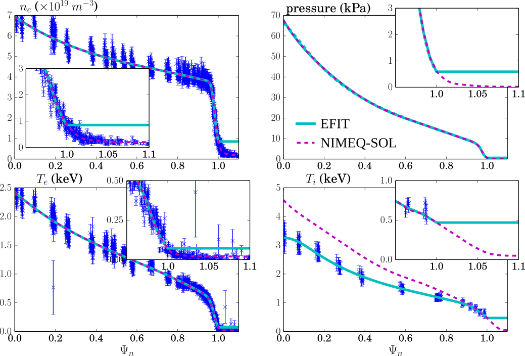
Figure 3: [color online] Fitted profiles (lines) from the Thompson (electron density and temperature) and CER (ion temperature) data from shot 160414 at 3025 ms. The solid lines are fits to raw data inside the LCFS where total pressure is computed from the measured species’ data and includes contributions from energetic particles. The dashed lines are the fits that include the SOL region and dashed ion temperature is computed after constraint by a two temperature model and quasineutrality.

In order to demonstrate and quantify the impact of our methods that recompute the Grad-Shafranov solution and add SOL-profile gradients, we choose two specific cases to study in detail: a low SOL-current case and a high SOL-current case. The first of these cases is an efit reconstruction of DIII-D shot 160414 at 3025 ms with profiles as shown in Fig. 3. Profiles are specified as function of normalized flux. The profiles shown are as included from the efit reconstruction and for fits with SOL-profile gradients (nimeq-SOL) along with the experimental Thomson and CER measurements . This shot is from an experiment of lithium pellet injection for edge-localized-mode pacing and the specific time represents the last 20% of the inter-ELM period. The reconstruction contains a relatively cold plasma at the LCFS, and thus a small pressure gradient in the fitted profiles within the SOL region. This implies modest SOL current and modification to the resulting equilibria when the SOL profiles are included in the Grad-Shafranov solve. In particular, at the LCFS $T_{e}=72$ eV, $T_{i}=470$ eV and $n_{e}=8.6\times 10^{18}$ $m^{-3}$ and in the current-free region $T_{e}=20$ eV, $T_{i}=50$ eV and $n_{e}=2.1\times 10^{18}$ $m^{-3}$ where the latter values only apply to equilibria with SOL-profile gradients.

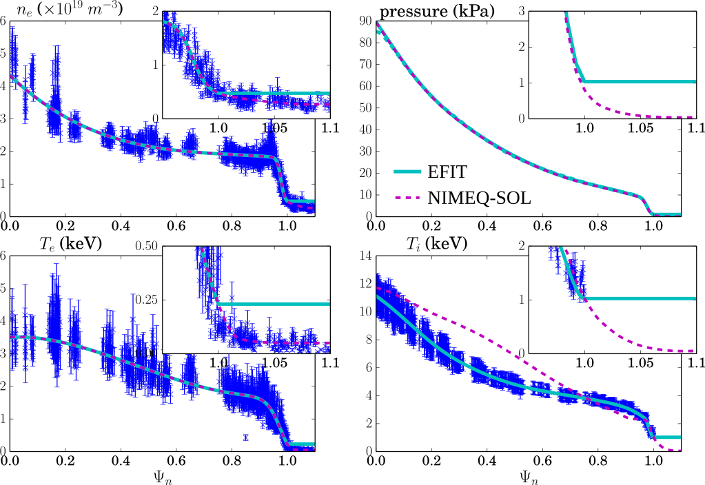
Figure 4: [color online] Fitted profiles (lines) from the Thompson (electron density and temperature) and CER (ion temperature) data from shot 145098 at 1800 ms. The solid lines are fits to raw data inside the LCFS where total pressure is computed from the measured species’ data and includes contributions from energetic particles. The dashed lines are the fits that include the SOL region and dashed ion temperature is computed after constraint by a two temperature model and quasineutrality.

The second case studied is an efit reconstruction of DIII-D shot 145098 at 1800 ms as shown in Fig. 4. Again, the profiles shown are as included from the efit reconstruction and for fits with SOL-profile gradients (nimeq-SOL) along with the experimental Thomson and CER measurements. This shot is from a DIII-D QH-mode experiment with ITER-like shaping during a period with edge harmonic oscillations (low-$n_{\phi}$ perturbations). This shot contains a relatively large pressure gradient from the fitted profiles in the SOL region. Thus relative to the reconstruction from shot 160414, we expect greater modifications to the equilibria resulting from the inclusion of the SOL-profile gradients in the Grad-Shafranov solve. In particular, at the LCFS $T_{e}=230$ eV, $T_{i}=1020$ eV and $n_{e}=4.8\times 10^{18}$ $m^{-3}$ and in the current-free region $T_{e}=50$ eV, $T_{i}=50$ eV and $n_{e}=2.7\times 10^{18}$ $m^{-3}$ where the latter values only apply to equilibria with SOL-profile gradients.

As is clear from Figs. 3 and  4, the nimeq-SOL ion-temperature profiles do not match the CER measured data. This is a consequence of a two-temperature model which over-constrains the profiles. Specifically, with a two-temperature model assuming quasi-neutrality ($n_{e}=Z_{i}n_{i}$) only the electron and ion fluids contribute to the pressure:

$$p^{2T}=p_{e}+p_{i}=n_{e}T_{e}+\frac{n_{e}}{Z_{i}}T_{i}^{2T}\;.$$ (3)

Thus only three of the four profiles shown in the figures ($n_{e}$, $p$, $T_{e}$, and $T_{i}$) can be matched exactly. Initializing computations with the measured pressure profile is essential as both the Grad-Shafranov solution and ideal stability are critically dependent on this profile. Secondary to this, the electron temperature profile determines the resistivity profile and the density profile sets Alfvén speed (among other collisionality parameters).

Within the context of an extended-MHD simulation, the ion-temperature profile typically becomes significant only when a two-fluid model is evolved and thus is often allowed to vary with respect to experimental measurements. In experiment, the pressure has contributions from both impurities and non-Maxwellian, or ‘hot’, ion particles from neutral-beam injection:

$$p=p_{e}+p_{i}+p_{imp}+p_{hot}=n_{e}T_{e}+n_{i}T_{i}\\ +\sum_{j}^{imp}n_{j}T_{j}+\sum_{h}^{hot}n_{h}T_{h}\;.$$ (4)

Comparing Eqns. (3) and (4), the ion temperature used to initialize our simulations includes the contributions from the other species:

$$T^{2T}_{i}=T_{i}\ +\sum_{j}^{imp}\frac{n_{j}Z_{i}}{n_{e}}T_{j}+\sum_{h}^{hot}\frac{n_{h}Z_{i}}{n_{e}}T_{h}\;.$$ (5)

As expected from this relation and as shown in the plots, the nimeq-SOL ion temperature (equivalent to $T^{2T}_{i}$ in Eqn. (5)) over estimates the measured ion temperature. For these cases, $Z_{i}$ is chosen such that the edge ion-temperature profile approximately matches the measured data within Figs. 3 and 4 ($Z_{i}=1.25$) . Thus computations in this work use the nimeq-SOL fits for $\psi_{n}<1$ and only the computations with SOL-profile gradients use the nimeq-SOL fits where $\psi_{n}>1$. Modeling that includes separate species for hot particles and/or impurities is required to eliminate the discrepancy with the measurements in the ion-temperature profile, and is thus planned for future study.

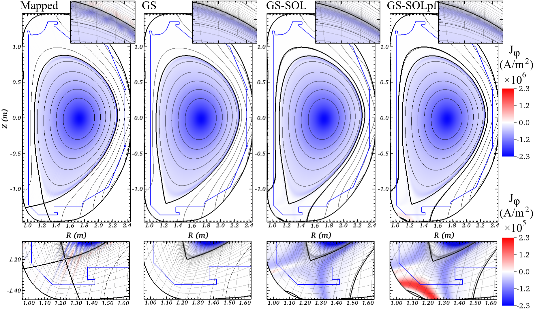
Figure 5: [color online] Toroidal current density from shot 160414 at 3025 ms plotted with LCFS, SOL (if applicable) and DIII-D limiter contours for four different cases: a mapped solution (using a finite-element computation for $\mathbf{B}$ and $\mathbf{J}$), resolving the Grad-Shafranov equation (GS), and resolving the Grad-Shafranov equation with two different treatments of the SOL (labeled GS-SOL and GS-SOLpf) as described in the text. The zoomed plots of the divertor region use a $10\times$ smaller contour color scale to show current features.

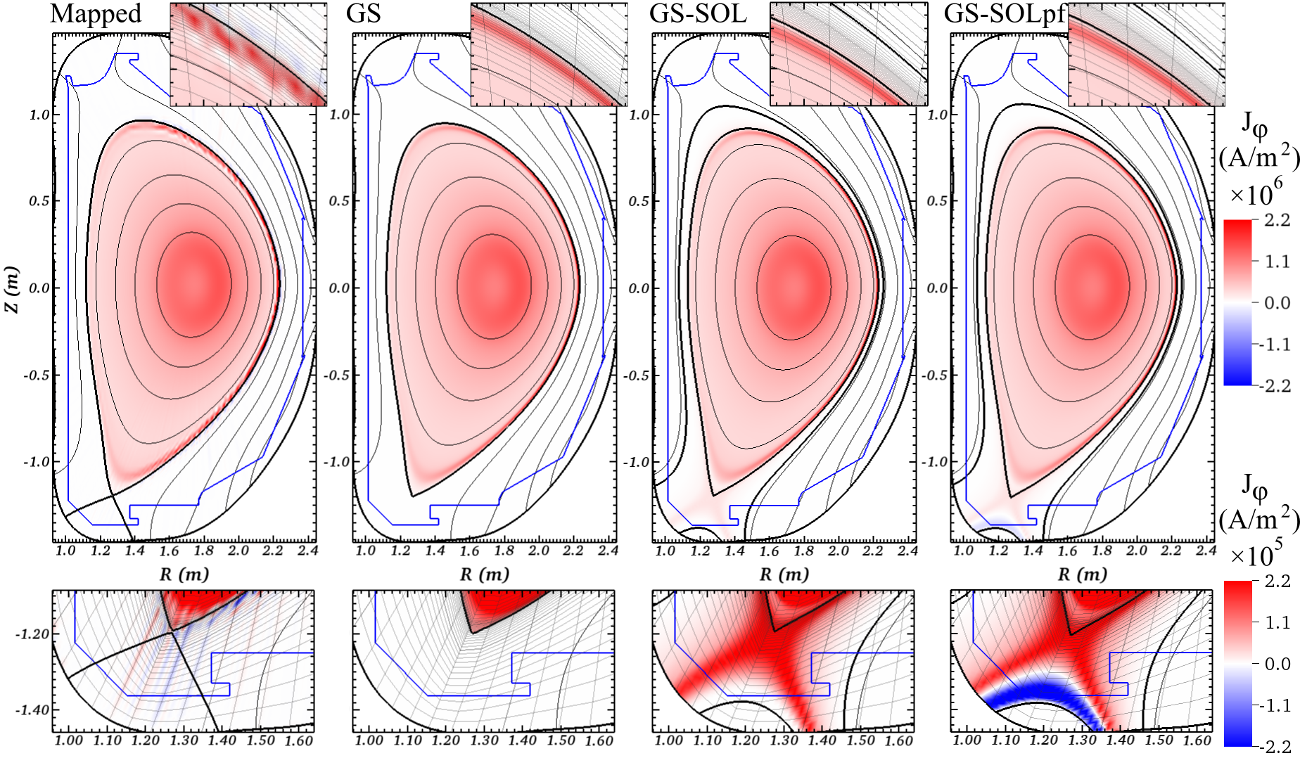
Figure 6: [color online] Toroidal current density from shot 145098 at 1800 ms plotted with LCFS, SOL (if applicable) and DIII-D limiter contours for four different cases: a mapped solution (using a finite-element computation for $\mathbf{B}$ and $\mathbf{J}$), resolving the Grad-Shafranov equation (GS), and resolving the Grad-Shafranov equation with two different treatments of the SOL (labeled GS-SOL and GS-SOLpf) as described in the text. The zoomed plots of the divertor region use a $10\times$ smaller contour color scale to show current features.

To further examine the reduction of mapping errors through the recomputation of the Grad-Shafranov solution, Figs. 5 and 6 show the resulting current-density distributions from the mapped and recomputed (GS) cases without SOL-profile gradients, along with two cases with SOL-profile gradients that are discussed later in this section, based on reconstructions from shots 160414 and 145098, respectively. The DIII-D first wall, LCFS and SOL contours are superimposed into the plotted computational domains. Shot 145098 uses a reversed plasma current relative to 160414, which uses the standard current orientation for DIII-D. These cases use a $72\times 64$ high-order finite-element mesh with bi-quartic elements. For both reconstructions, the mapped current is clearly distorted and contains numerical oscillations. This is particularly evident for the edge current shown in the zoomed insets of the figures and outside the LCFS as shown in the inset figures that magnify the details near the X-point. The numerical bumps in the current profiles inside the LCFS are a result of the mapping and are associated with the resolution of the efit grid. They are not eliminated but rather only resolved with enhanced nimeq resolution (see Fig. 1. While it is possible to partially circumvent this issue with the closed-flux mapped current by using a high-resolution efit (see, for example, Ref. Aiba et al. (2007); King et al. (2016)), in practice most efit reconstructions are generated at relatively low resolution relative to what is required for extended-MHD computations. The spatial requirements to solve for Grad-Shafranov equilibria are less stringent than those to solve for 3D MHD perturbations where, for example, the edge computations presented in Sec. VI use a finite element grid with $72\times 512$ with high-order bi-quintic elements. The current outside the LCFS in the mapped case results from the representation of the discontinuous current profile on nimeq’s $C^{0}$ finite-element spatial discretization. The mapped plots in Figs. 5 and 6 are generated with finite-element calculations that compute the poloidal magnetic field and current from the mapped $\psi$ and $RB_{\Phi}$ fields. Alternatively, splines may be used to map the poloidal magnetic field and current density. While this method produces smooth, but not consistent, fields, the derivatives of these fields with nimeq’s $C^{0}$ finite-element representation are used in extended-MHD calculations. Thus mapped magnetic fields and current densities with a spline spatial representation in effect hide, but do not eliminate, the mapping errors.

For the presented cases with SOL current, we use $\psi_{n,sol}=1.1$ and $\psi_{n,pf}=0.96$ in the fits to the electron density and temperature profiles from Thomson scattering measurements and extrapolate the ion temperature to an assumed $50eV$. The resulting profiles are shown as the dashed purple line in Figs. 3 and 4. The half width of the electron pressure profiles are roughly $3.3\;mm$ and $2.7\;mm$ at the outboard mid-plane and $7.3\;cm$ and $4.7\;cm$ at the divertor plate for the cases from shots 160414 and 145098, respectively. This results in SOL widths that are roughly consistent with the measured half width of the heat-flux during the later half of the inter-ELM period of DIII-D ELMy H-mode discharges in Ref. Eich et al. (2013).

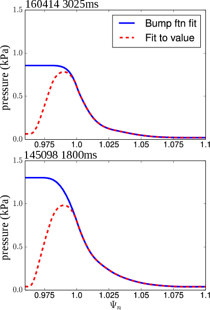
Figure 7: [color online] Fitted pressure profiles in the SOL and private-flux region with two different fits, one with bump function fits in the private-flux region (SOL case) and the second with a fit that specifies a low pressure at the edge of the private-flux region (SOLpf case), for two different shots, 160414 at 3025ms (top) and 145098 at 1800 ms (bottom).

Currently, we do not have diagnostic information about appropriate profiles for the private-flux region. Two methods employing the bump function extrapolations are compared with profiles shown in Fig 7. In the first method, $C^{2}$ continuity is enforced at $\psi_{n}=1$ resulting in a high-pressure, high-density private-flux region. With the second method, $C^{1}$ continuity is enforced at $\psi_{n}=1$ and the values at $\psi_{pf}$ are set to the same as those at $\psi_{sol}$. In the figures and tables, these cases are referred to as GS-SOL and GS-SOLpf, respectively. The profiles generated with the second method (GS-SOLpf) roughly match the measured heat-flux profile Groebner et al. (2011); Eich et al. (2013).

In addition to the mapped and recomputed cases without SOL current, Figs. 5 and 6 plot cases with SOL currents. With low pressure in the private-flux region the toroidal current density reverses locally near the divertor strike points after the Grad-Shafranov solve as shown in the inset figure for the GS-SOLpf case. Currents near and outside the limiter are likely an artifact of our method. In this cold-plasma region, additional terms in the momentum equation become large (e.g. interactions with neutrals and the first wall) that are outside the scope of the Grad-Shafranov equation. As such, the approximation that quatities are functions of the flux surfaces breaks down. However, at present our focus is on the effects of the SOL-profile gradients near the LCFS where there is the potential for interaction with perturbations that originate from inside the separatrix. With SOL-profile gradients, there is a modest modification (less than 1%) to the plasma current. For the cases shown here, we re-normalize the total current to match the value from the efit reconstruction using the method of Ref. Lütjens et al. (1996). Cases with and without current re-normalization produce similar results, where the $\chi^{2}$ values discussed in the Sec. V are slightly smaller for cases with re-normalization.

The poloidal current in the SOL that flows into and out of the divertor plate are solely an effect of the profile gradient in the toroidal magnetic flux within the SOL. For these cases, a bump-function fit that enforces $C^{2}$ continuity at $\psi_{n}=1$ determines the toroidal-magnetic-flux profile in the SOL. The resulting poloidal currents have a maximum value on the divertor plate of 4000 and 500 $A/m^{2}$ for the cases from shots 160414 and 145098, respectively. This current must be less than the ion saturation current ($J_{max}=n_{e}ec_{s}$). With a Deuteron ion species, a conservative calculation of the ion saturation current (using the vacuum temperatures and densities from each case) is over $2\times 10^{4}$ $A/m^{2}$ for both cases.

V Synthetic diagnostics

Analysis between each nonlinear Grad-Shafranov-solve iteration provides a confirmation that the macroscopic quantities of the equilibrium (e.g. total current, toroidal flux and internal energy) are invariant between the mapped equilibrium and the new solution. In the interest of showing that our methods which recompute the Grad-Shafranov equilibrium and add SOL profiles and current only minimally impact the relative agreement with measurements, we use a more advanced comparison that computes a $\chi^{2}$ value. The Python code nimnostics is used to calculate a $\chi^{2}$ from the shots and sub-cases previously discussed. nimnostics models the magnetic coils, MSE and Thomson scattering through local evaluations of the fields where linear interpolation is used between finite-element nodes. Thus the boundary of the domain is chosen as the approximate vacuum vessel instead of the limiter in order to encompass the magnetic coil locations for comparison.

Table 1: Values of $\chi^{2}/N$, where $N$ is the number of measurements, for each diagnostic for the reconstruction, change in plasmas current relative to the efit value (-1178772 Amps), and change in the X-point and maximum Z value of the LCFS for shot 160414 at 3025ms.

$\chi^{2}/N$	mapped	GS	GS-SOL	GS-SOLpf
Thom. $T_{e}$	22.3	23.4	4.80	4.15
Thom. $n_{e}$	19.4	20.5	4.07	3.33
CER $T_{i}$	6.98	6.96	6.74	6.84
MSE	1.49	1.49	1.46	1.47
Mag. Coils	0.61	0.63	0.82	0.70
$\Delta$s	mapped	GS	GS+SOL	GS+SOLpf
$\Delta I/I_{0}$	6.95$\times 10^{-5}$	7.97$\times 10^{-4}$	3.22$\times 10^{-7}$	3.22$\times 10^{-7}$
$\Delta\mathbf{r}_{xpt}$ (cm)	N/A	ref.	0.72	1.07
$\Delta\mathbf{r}_{zmax}$ (cm)	N/A	ref.	0.35	0.19

Table 2: Values of $\chi^{2}/N$, where $N$ is the number of measurements, for each diagnostic for the reconstruction, change in plasmas current relative to the efit value (1063788 Amps), and change in the X-point and maximum Z value of the LCFS for shot 145098 at 1800ms.

$\chi^{2}/N$	mapped	GS	GS-SOL	GS-SOLpf
Thom. $T_{e}$	60.9	61.7	7.77	6.99
Thom. $n_{e}$	2.87	5.22	11.4	9.93
CER $T_{i}$	10.2	10.3	19.7	19.6
MSE	1.14	1.13	1.13	1.13
Mag. Coils	1.65	1.60	4.57	3.27
$\Delta$s	mapped	GS	GS+SOL	GS+SOLpf
$\Delta I/I_{0}$	9.86$\times 10^{-5}$	5.46$\times 10^{-3}$	-3.57$\times 10^{-7}$	-3.57$\times 10^{-7}$
$\Delta\mathbf{r}_{xpt}$ (cm)	N/A	ref.	0.86	0.55
$\Delta\mathbf{r}_{zmax}$ (cm)	N/A	ref.	2.82	2.12

Summaries of the $\chi^{2}$ value by diagnostic and case for the reconstructions from shots 160414 and 145098 are shown in Tabs. 1 and 2, respectively. In both shots, the mapped and recomputed equilibria without SOL-profile gradients (GS cases) are roughtly equivalent indicating that the equilibrium resulting from the recomputation is substantially similar. For the cases with modest SOL-profile gradients and currents (shot 160414), the $\chi^{2}$ values for a given measurement either decreases and the deviations of the LCFS contour are modest or are roughly the same as the mapped and GS cases. However, cases from the shot with large SOL current and profile gradients exhibit mixed results with some measurements decreasing in $\chi^{2}$ (Thomson electron temperature) and others increasing in $\chi^{2}$ (Thomson electron density, MSE and coils) when comparing relative to the mapped and GS cases. The deviation of the LCFS contour is also as much as 2 cm on the upper side of the contour. This deviation is apparent in the inset figures of Fig. 6.

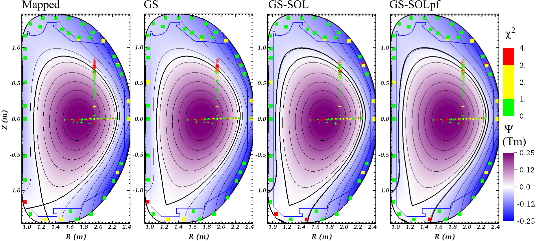
Figure 8: [color online] Values of $\chi^{2}$ from different local measurements (crosses are from Thomson measurements of electron density, diamonds are from MSE measurements, and squares are from coil measurements of the poloidal magnetic field) plotted with a color plot of the $\psi$ solution and LCFS, SOL (if applicable) and DIII-D limiter contours from shot 160414 at 3025 ms for four different cases: a mapped solution (using a finite-element computation for $\mathbf{B}$ and $\mathbf{J}$), resolving the Grad-Shafranov equation (GS), and resolving the Grad-Shafranov equation with two different treatments of the SOL (GS-SOL and GS-SOLpf) as described in the text.

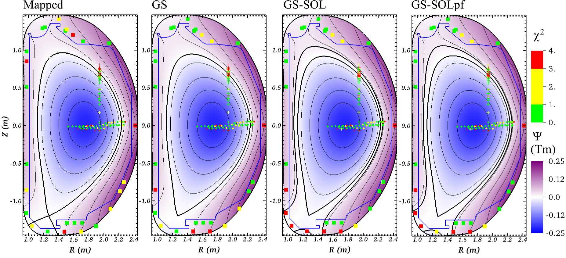
Figure 9: [color online] Values of $\chi^{2}$ from different local measurements (crosses are from Thomson measurements of electron density, diamonds are from MSE measurements, and squares are from coil measurements of the poloidal magnetic field) plotted with a color plot of the $\psi$ solution and LCFS, SOL (if applicable) and DIII-D limiter contours from shot 145098 at 1800 ms for four different cases: a mapped solution (using a finite-element computation for $\mathbf{B}$ and $\mathbf{J}$), resolving the Grad-Shafranov equation (GS), and resolving the Grad-Shafranov equation with two different treatments of the SOL (GS-SOL and GS-SOLpf) as described in the text.

In order to examine the source of the changes in $\chi^{2}$ in detail, Figs. 8 and 9 show the local values of $\chi^{2}$ from Thomson electron density, MSE and magnetic coils measurements for our four different cases on shots 160414 and 145098, respectively. With shot 160414 the aggregate $\chi^{2}$ values are improved or comparable for every diagnostic when comparing the cases with SOL gradients to those without (as seen in Tab. 1). We note that $\chi^{2}$ values are particularly improved with SOL-profile gradients for the Thomson measurements, and Fig. 8 shows that this is a result of improved agreement in the SOL region. The results are mixed for shot 145098 (as seen in Tab. 2). While the aggregate $\chi^{2}$ value for the Thompson electron temperature profile improves when SOL-profile gradients are included, the $\chi^{2}$ value for the Thomson electron density profile is degraded. Examination of Fig. 9 shows that while the $\chi^{2}$ values in the SOL region are smaller when the SOL-profile gradients are included, the values near the LCFS become large consistent with the approximately 2 cm movement of the separatrix line relative to the cases without SOL-profile gradients. Additionally, the $\chi^{2}$ values for the magnetic-coil measurements become marginally larger near the divertor region as these values are affected by the inclusion of toroidal current in this region.

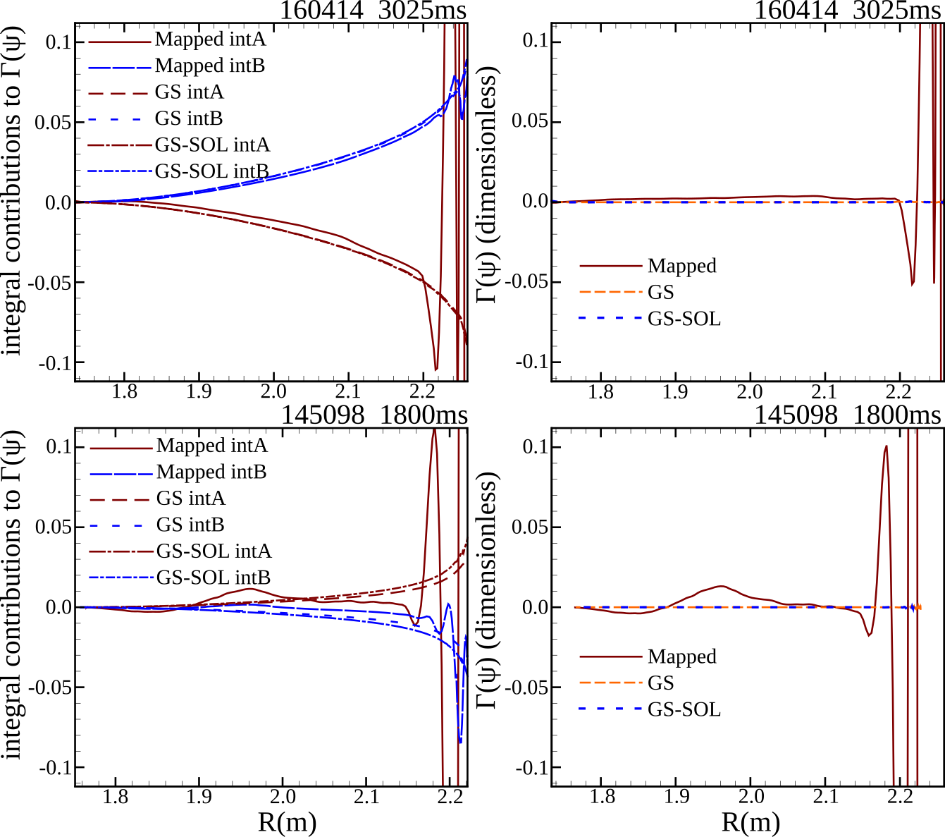
Figure 10: [color online] The flux-surface-averaged geometrical quantity of Eqn. (6) from Ref. Ramos (2015a), $\Gamma(\psi)$ (right), and decomposition by integral contributions from the two integrals in the expression (left) which are referred to as intA and intB, respectively. Figures from both example cases, shot 160414 (top) and 145098 (bottom), are shown. The integral vanishes analytically, and this behavior is only reproduced numerically with recomputation of the Grad-Shafranov solution.

As an additional test of the quality of the equilibrium, we calculate the flux-surface-averaged geometrical quantity discussed in Ref. Ramos (2015a),

$$\Gamma(\psi)=2\frac{d}{d\psi}\oint dl\mathbf{B}\cdot\nabla R^{2}\\ +\oint\frac{dl}{B}[2\mathbf{b}\cdot\nabla(\nabla\psi\cdot\nabla lnR^{2})+\nabla\psi\cdot\nabla(\mathbf{b}\cdot\nabla ln|B|)]$$ (6)

where $\mathbf{b}=\mathbf{B}/|B|$. Figure 10 shows the result of this calculation and the decomposition of the expression in Eqn. (6) into separate contributions from the two integrals in the expression (referred to as intA and intB, respectively) for both shots examined in our studies. This integral is known to vanish analytically Ramos (2015b), however this behavior is only reproduced numerically with recomputation of the Grad-Shafranov solution. Consistent with the relatively large motion of the flux surfaces ($2-3\;cm$) in the large SOL-current case (145098), the contributing integrals for this case differ slightly between the GS and GS-SOL cases where only the latter includes the SOL current. The contributing integrals lie on top of each other for the low SOL-current case (160414). The improved equilibria provided by recomputation of the Grad-Shafranov solution are critical in NIMROD drift-kinetic computations Held et al. (2015). For example, an accurate account of $\mathbf{b}\cdot\nabla ln|B|$ in latter integral of Eqn. (6) (intB) is essential when assessing how trapped particles affect parallel closures for NIMROD’s fluid system.

VI Effect on linear peeling ballooning modes

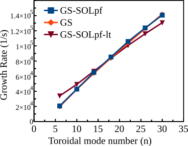
Figure 11: [color online] Growth rates vs. toroidal mode from shot 145098 at 1800 ms with and without SOL current. The presence of the SOL current does not modify the growth rate (compare GS-SOLpf and GS cases). The GS-SOLpf-lt case is a modification to the SOLpf case with $T_{e}=1$ eV at the edge of the SOL. The low edge temperature enhances the vacuum response Burke et al. (2010); Ferraro et al. (2010) and modestly modifies the growth rate.

In order to assess the impact, if any, on linear stability we examine the toroidal-mode-number ($n_{\phi}$) growth-rate spectrum for shot 145098 at 1800 ms with and without SOL-profile gradients. The reconstruction from shot 160414 is during a stable inter-ELM period and thus it is not considered. As seen in Fig. 11, the growth rates are only minimally impacted by the inclusion of SOL-profile gradients where the difference between the growth rates is at most 5% (at $n_{\phi}=6$). A $72\times 512$ mesh with bi-quintic elements is used for these computations. The growth rates with the SOL current are larger than those without for $n_{\phi}<30$ and 1% smaller at $n_{\phi}=30$. This is consistent with the effect of enhanced resistivity and decreased density outside the LCFS as associated with the SOL-profile gradients that leads the dynamics in this region to produce a more vacuum-like response (see Refs. Burke et al. (2010); Ferraro et al. (2010)) whereby the low-$n_{\phi}$ modes are destabilized and the high-$n_{\phi}$ modes are stabilized. In order to investigate this response further, we examine a case with a low electron temperature, 1 eV, at the edge of the SOL region (annotated as GS-SOLpf-lt in the figure). The stabilizing effect at low $n_{\phi}$ and destabilization at high $n_{\phi}$ from the enhanced vacuum-like response is more apparent for this case. Relative to the case without SOL current, the growth rates for this case are 7% larger at $n_{\phi}=6$ and 8% smaller at $n_{\phi}=30$. Thus the effect of the SOL-profile gradients is modest compared to the effect of drift-stabilization (see e.g. Refs. King et al. (2016); King and Kruger (2014)) - a result that is consistent with prior PBM calculations Snyder et al. (2002).

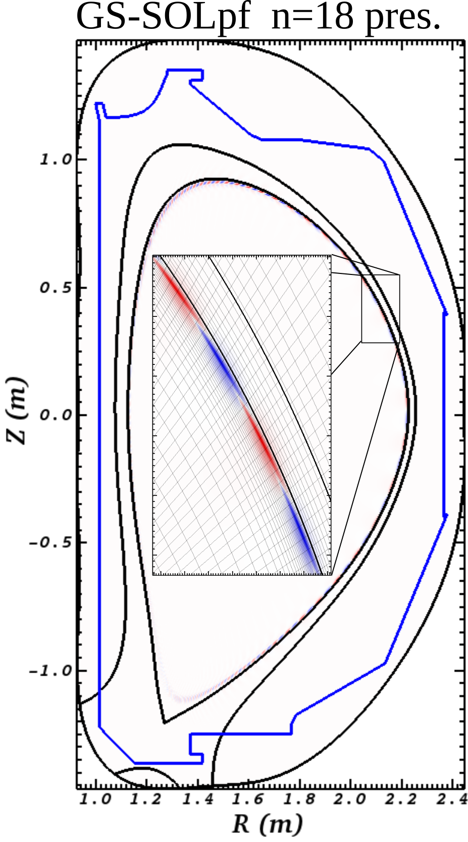
Figure 12: [color online] Pressure contours (arbitrary units) from an extended-MHD calculation of a $n_{\phi}=18$ mode during shot 145098 at 1800 ms where SOL current is included in the equilibrium. The localization within the LCFS is consistent with the small effect of the SOL current on the mode.

As seen in Fig. 12, the mode structure is localized within the region just inside the LCFS. Convergence is affected by discontinuity in the current-density profile when SOL-profile gradients are not included even though the mode is localized away from this discontinuity. nimrod does not enforce the $\nabla\cdot B=0$ constraint through the spatial discretization, but rather converges to a solution with small $\nabla\cdot B$ error. The $\ell^{2}$-norm of $\nabla\cdot B$ is reduced by approximately 50% in the cases with SOL-profile gradients relative to cases without as a result of the continuous equilibrium profiles.

VII Discussion and Conclusions

Relative to the effect on linear computations (Sec. VI), the inclusion of SOL-profile gradients and associated continuous current-density profiles has a greater impact on nonlinear modeling with perturbations that are advected across the separatrix such as the studies of QH-mode evolution of Ref. King et al. (2017). Nonlinear computations can be affected by the inclusion of SOL-profile gradients in multiple ways: the spatial resolution required to converge on the dynamics at the LCFS is less with a continuous current profile as the dynamics are affected by discontinuities in the current and by the changes in the vacuum-like response as described in Sec. VI.

Perhaps more importantly, the methods described to extrapolate the thermodynamic profiles in the SOL can be applied to modeling with flows. Typically, the measured flows do not vanish at the LCFS and can be extrapolated to zero in the SOL region. Including this extrapolation both affects the dynamics of the perturbations as they cross the LCFS and prevents the computationally pathological case where perturbations may be advected quickly inside the LCFS and not at all outside. Again, an example that applies these methods to modeling with flows is found in Ref. King et al. (2017).

The inclusion of SOL-profile gradients may have an effect outside the context of modeling with initial value codes. The last-closed flux-surface locations are shifted by up to $3\;cm$ in the cases included in this study. While this shift may not greatly affect MHD stability, it could have an impact on methods that are predicated on highly accurate reconstructions such as RF injection for current drive and/or tearing mode stabilization. These considerations may motivate the inclusion of the SOL-profile gradients within the reconstruction itself.

One limitation to the methods described here is that the flux from the plasma that penetrates through the walls remains fixed. The flux can be decomposed into plasma and external-coil contributions ($\psi=\psi_{plasma}+\psi_{ext.coil}$). A potential extension to this work is to perform a free-boundary computation where $\psi_{ext.coil}$ is fixed but $\psi_{plasma}$ is allowed to vary. Additionally, $\psi_{ext.coil}$ could be extended to include contributions from return currents flowing through the wall. Ultimately, as these computations become more sophisticated it may be better to include the SOL-profile gradients in the $\chi^{2}$ minimization performed during the reconstruction.

Even with this caveat, our methods represent substantial progress on the initial condition for edge modeling. In particular, we have developed a workflow whereby SOL-profile gradients and current can be included in the initial condition for nimrod even if they are not included in the reconstruction. Using both global (e.g. total current) and local (e.g. the separatrix location) metrics as well as a $\chi^{2}$ test we quantify the impact of our methods on the accuracy of the initial condition after inclusion of SOL-profile gradients. We find that this impact is small and that the modified initial condition closely resembles the state found by the reconstruction. While linear stability is modestly impacted by the inclusion of the SOL-profile gradients through an enhancement of the vacuum-like response, we argue that our methods are more important for nonlinear modeling of dynamics across the separatrix.