Flavor-dependent neutrino angular distribution in core-collapse supernovae

Abstract

According to recent studies, the collective flavor evolution of neutrinos in core-collapse supernovae depends strongly on the flavor-dependent angular distribution of the local neutrino radiation field, notably on the angular intensity of the electron-lepton number carried by neutrinos. To facilitate further investigations of this subject, we study the energy and angle distributions of the neutrino radiation field computed with the Vertex neutrino-transport code for several spherically symmetric (1D) supernova simulations (of progenitor masses 11.2, 15 and 25 $M_{\odot}$) and explain how to extract this information from additional models of the Garching group. Beginning in the decoupling region (“neutrino sphere”), the distributions are more and more forward peaked in the radial direction with an angular spread that is largest for $\nu_{e}$, smaller for $\bar{\nu}_{e}$, and smallest for $\nu_{x}$, where $x=\mu$ or $\tau$. While the energy-integrated $\nu_{e}$ minus $\bar{\nu}_{e}$ angle distribution has a dip in the forward direction, it does not turn negative in any of our investigated cases.

MPP-2017-9, INT-PUB-17-007

1. Introduction

Neutrinos are the main agents of energy and lepton-number transport in core-collapse supernovae (SNe). Within the delayed explosion mechanism of Bethe and Wilson, neutrinos cause the explosion by shock reheating and determine nucleosynthesis yields (Janka, 2012; Burrows, 2013). Neutrinos will also allow us to monitor core-collapse phenomenology when high event statistics will be collected by existing and future large-volume detectors in the event of a nearby SN explosion (Scholberg, 2012).

The energies and densities in core-collapse environments are of typical nuclear-physics scales, i.e., $\mu$ and $\tau$ leptons do not exist except perhaps for some muons in the hottest regions. Hence, heavy-lepton neutrinos, often collectively called $\nu_{x}$, mostly interact by neutral-current processes, whereas $\nu_{e}$ and $\bar{\nu}_{e}$ interact predominantly by $\beta$ reactions. Neutrino transport, emission, and their detection therefore have a pronounced flavor dependence.

Developing a reliable theoretical understanding of neutrino flavor evolution in astrophysical environments with high neutrino density has been surprisingly difficult because of neutrino-neutrino refraction (Duan et al., 2006, 2010; Mirizzi et al., 2016; Chakraborty et al., 2016a). Flavor evolution is here a dynamical phenomenon as neutrinos feed back upon themselves, i.e., one needs to study collective flavor degrees of freedom of the entire ensemble, not only of individual neutrinos or individual momentum modes. These collective modes can show instabilities such that flavor conversion can occur even in regions where the large matter effect suppresses normal flavor oscillations of individual modes. One generic type of process is pair conversion $\nu_{e}\bar{\nu}_{e}\leftrightarrow\nu_{x}\bar{\nu}_{x}$ on the forward-scattering (refractive) level. It does not violate flavor-lepton number and of course proceeds anyway by normal non-forward scattering, but can be collectively enhanced even without neutrino flavor mixing.

For the neutrino energies relevant in collapsed stars, the weak processes are usually described by the four-fermion interaction proportional to the Fermi constant $G_{\rm F}$. The space-time structure is of current-current form and implies that the interaction energy between relativistic neutrinos is proportional to $(1-\cos\vartheta)$, where $\vartheta$ is their relative angle of propagation. In particular, parallel-moving neutrinos have no mutual refractive effect at all. Therefore, in this context, we cannot treat neutrinos as flowing in a purely radial direction.

To account for the crucial neutrino angle distribution, one often adopted a simple “bulb model” of neutrino emission (Duan et al., 2006). It consists of an emitting surface, the “neutrino sphere,” as a source of flavor-dependent neutrino spectra with a common angle distribution. The latter was often taken to be black-body like, i.e., isotropic into the outer half-space, or in the form of “single-angle emission,” i.e., only one zenith angle of emission relative to the local radial direction with local axial symmetry. Some tentative studies used different local angle distributions between $\nu_{x}$ and a common one for $\nu_{e}$ and $\bar{\nu}_{e}$ in a schematic way (Mirizzi & Serpico, 2012). On the other hand, non-trivial angle distributions, especially between $\nu_{e}$ and $\bar{\nu}_{e}$, may be crucial for a full appreciation of flavor evolution (Sawyer, 2005, 2009, 2016; Chakraborty et al., 2016b; Dasgupta et al., 2017; Izaguirre et al., 2017; Wu & Tamborra, 2017).

At large distances from the SN core, the neutrino flux is essentially a narrow “beam” with small opening angle. In addition, residual scattering provides a wide-angle “halo” which has low intensity, yet it is responsible for a non-negligible contribution to the $(1-\cos\vartheta)$ term (Cherry et al., 2012; Sarikas et al., 2012b). By the same token, a “backward” flux toward the SN core exists and is particularly important near the decoupling region where neutrinos flow in all directions with different intensities. Therefore, a simple treatment of flavor evolution as a function of radius with only an inner boundary condition at the arbitrarily defined “neutrino sphere” does not necessarily capture this physical situation (Izaguirre et al., 2017). Moreover, if the $\nu_{e}$ and $\bar{\nu}_{e}$ distributions are sufficiently different, “fast flavor instabilities” can ensue. The latter do not depend on neutrino mass differences and, specifically, are driven by the angle distribution of the electron lepton number (ELN) carried by neutrinos.

Despite the role played by neutrino angle distributions in the flavor evolution, it is difficult to glean enough insight about them from the published literature on numerical SN simulations. The basic picture of how neutrinos interact and decouple tells us that the $\nu_{e}$ distribution should be broader than that of $\bar{\nu}_{e}$, and both broader than that of $\nu_{x}$. However, to mimic the local radiation field at some distance $r$ by assuming these flavors are emitted by different neutrino spheres, i.e., a separate “bulb model” for each species, for sure is overly simplistic, especially close to the SN core where backward propagating neutrinos are important as well.

The main point of our paper is to fill this gap in the literature and to provide a first overview of neutrino energy and angle distributions. In this way we hope to provide crucial input information for further studies of collective neutrino flavor evolution. In particular, we present angle-dependent distributions from hydrodynamical simulations of three SN progenitors with masses of 11.2, 15 and $25\,M_{\odot}$ and characterize their variation as a function of the distance from the core. These models were developed by Hüdepohl (2013) with the 1D version of the Garching group’s Prometheus-Vertex code.

In principle, it would be desirable to provide neutrino distributions from 3D models. One expects an even richer phenomenology and a greater diversity of cases regarding the local neutrino distributions. However, the numerical approximations used in state-of-the-art 3D simulations (such as ray-by-ray or two-moment closure schemes) are not qualified to provide reliable neutrino angle distributions. Solutions of the Boltzmann transport equation in 3D are needed to obtain full phase-space information for the neutrinos. Corresponding methods, however, are still being developed. First results for static and stationary conditions in 3D (Sumiyoshi et al., 2015) and time-dependent simulations in 2D (Ott et al., 2008; Brandt et al., 2011; Nagakura et al., 2017) with multi-angle transport are available, but still suffer from major shortcomings, e.g. the lack of energy-bin coupling (Ott et al., 2008; Brandt et al., 2011), and coarse resolution, especially in the momentum space. Therefore, studies similar to the one presented here, but for 3D models, will have to wait for the next generation of 3D SN simulations including Boltzmann neutrino transport, which will require exascale computing.

In Sec. 2 we introduce our models and in Sec. 3 we describe the angle-integrated features of the neutrino field and their variations as functions of radius. In Sec. 4 we study the neutrino distributions as functions of zenith-angle, radius, and post-bounce time. Conclusions and an outlook are provided in Sec. 5. Appendix A reports a glossary of the definitions usually adopted in neutrino radiative transport vs. the terminology more common in flavor oscillation studies. The neutrino angle distributions for our models are provided as supplementary material and instructions on how to use these data are provided in Appendix B.

2. Numerical supernova models

We will explore the characteristics of the neutrino radiation field during the accretion phase of three spherically symmetric SN simulations with progenitor masses 11.2, 15 and $25\,M_{\odot}$. The nuclear equation of state is from Lattimer & Swesty (1991) with compressibility modulus $K=220$ MeV (Hüdepohl, 2013). The simulations were performed with the 1D version of the Prometheus-Vertex code. It couples an explicit third-order Riemann-solver-based Newtonian hydrodynamics code with an implicit three-flavor, multi-energy group two-moment closure scheme for neutrino transport. The neutrino transport applied here used three species $\nu_{e}$, $\bar{\nu}_{e}$ and $\nu_{x}$ (with $\nu_{x}=\nu_{\mu},\nu_{\tau},\bar{\nu}_{\mu},\bar{\nu}_{\tau}$), and the variable Eddington-factor closure for the two-moment equations is obtained from a model Boltzmann equation, whose solution is based on a tangent-ray discretization and provides also information on the angle-dependent neutrino intensities (Rampp & Janka, 2002), which are of central importance for the present work.

General relativistic (GR) corrections are accounted for by using an effective gravitational potential (case A of Marek et al., 2006) and by including GR redshift and time dilation in the transport. The relatively small effects of GR ray bending in the NS environment, however, are ignored in the neutrino treatment, i.e., the tangent-ray method assumes neutrinos to propagate along straight paths instead of curved geodesics. Tests showed good overall agreement until several 100 ms after core bounce (Marek et al., 2006; Liebendörfer et al., 2005) with fully relativistic simulations of the Basel group’s Agile-Boltztran code. A more recent comparison with a GR program (Müller et al., 2010) that combines the CoCoNuT hydro solver (Dimmelmeier et al., 2002) with the Vertex neutrino transport, revealed almost perfect agreement except for a few quantities with deviations of at most 7–10$\%$ until several seconds. Our models presented here include the full set of neutrino reactions described in Appendix A of Buras et al. (2006) with the original references given there. (The simulation setup is analog to the “full” opacity case discussed in Hüdepohl et al. 2010.) In particular, we account for nucleon recoils and thermal motions, nucleon-nucleon (NN) correlations, weak magnetism, a reduced effective nucleon mass and quenching of the axial-vector coupling at high densities, NN bremsstrahlung, $\nu\nu$ scattering, and neutrino-antineutrino-pair conversions between different flavors (Buras et al., 2003). In addition, we include electron capture and inelastic neutrino scattering on nuclei (Langanke et al., 2003, 2008).

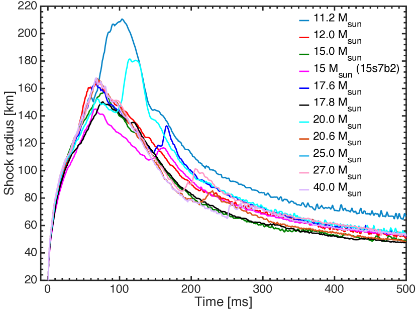
The progenitor models employed for our stellar core-collapse simulations are taken from Woosley & Weaver (1995) in the case of the 15 $M_{\odot}$ progenitor model s15s7b2 and from Woosley et al. (2002) for all other investigated cases. Figure 1 shows the evolution of the shock radius as a function of the post-bounce time. All the simulated models exhibit similar features; see also the angle-integrated neutrino emission properties shown in Fig. 7 of Janka et al. (2012). The 11.2 and the $25\,M_{\odot}$ progenitors gauge the maximum variation of the neutrino light curves of the broader simulated mass range of SN progenitors shown in Fig. 7 of Janka et al. (2012), while the $15\,M_{\odot}$ progenitor is an intermediate case.

Figure 1.— Shock radii as functions of post-bounce time for the progenitor models of Hüdepohl (2013). The model labelled as “15s7b2” corresponds to our benchmark case of 15 $M_{\odot}$.

For each of the three progenitors discussed here, we inspect the neutrino angle and energy distributions at three representative post-bounce times. These are chosen such as to represent the neutrino-field properties soon after the shock-breakout burst (early accretion phase), just before the drop in the luminosity due to the infall of the Si/SiO shell interface, usually occurring around 200 ms post bounce, and in the late accretion phase. The selected post-bounce times for each model are $t=61$, 250 and 550 ms for the $11.2\,M_{\odot}$ progenitor, $t=150$, 280 and 500 ms for $15\,M_{\odot}$, and $t=63$, 250 and 350 ms for $25\,M_{\odot}$. Unless otherwise specified, the $t=280$ ms snapshot of the $15M_{\odot}$ model will be used as a benchmark case.

The fundamental quantity to describe the neutrino radiation field for each flavor $\nu_{\alpha}=\nu_{e}$, $\bar{\nu}_{e}$ and $\nu_{x}$ is the spectral intensity $I_{E,\Omega}$ as explained in Appendix A, where we provide a glossary of different definitions used in neutrino radiative transport and in studies of neutrino flavor evolution. The spectral intensity is the energy of a given species $\nu_{\alpha}$ that streams at energy $E$ per unit time through a unit area in a unit solid angle around direction $\Omega$ perpendicular to the area. It has units ${\rm cm}^{-2}~{}{\rm s}^{-1}~{}{\rm ster}^{-1}$ (note that the energy units in numerator and denominator cancel). In spherically symmetric SN simulations, the intensity is axially symmetric. For each radial grid point $r_{i}$, the intensity is discretized at the zenith-angle points $\mu_{ij}$ (where $\mu=\cos\theta$) on a tangent-ray grid, i.e., the zenith-angle grid is different for different radial positions $r_{i}$ (Rampp & Janka, 2002). In our benchmark case, a maximum of 824 angular bins was used. The energy grid $E_{k}$ is made from 21 bins up to 380 MeV with nearly geometric spacing.

The quantity provided by our SN simulations is the monochromatic neutrino intensity for each flavor $\nu_{\alpha}$, integrated over the energy bin $[E_{k,\mathrm{min}},E_{k,\mathrm{max}}]$ centered on $E_{k}$

$$I_{ijk}=\int_{E_{k,\mathrm{min}}}^{E_{k,\mathrm{max}}}I_{E,\Omega}(r_{i},\mu_{ij},E)\,dE\,$$ (1)

in units of ${\rm MeV}~{}{\rm cm}^{-2}~{}{\rm s}^{-1}~{}{\rm ster}^{-1}$. Notice that the discrete variables $r_{i}$ and $E_{k}$ are at the center of their respective bins. In the following, we will define the corresponding discrete quantities for the neutrino field as directly connected to the numerical grid of the simulation.

Traditionally, SN neutrino flavor oscillation studies were concerned with relatively large distances and typically used a description of the neutrino field as seen by a distant observer. On the other hand, if we consider the neutrino-matter decoupling region, it may be more appropriate to use Lagrangian coordinates comoving with the local matter flow. The output quantities of the Garching simulations are given in this comoving frame and we will use it here as well.

Figure 2.— Radial variation of global properties of our benchmark case, the 280 ms snapshot of the $15\ M_{\odot}$ model. The blue, red and green lines are for $\nu_{e}$, $\bar{\nu}_{e}$ and $\nu_{x}$ as indicated. Left panels: Neutrino luminosity, number luminosity (or total number flux), and local number density. Right panels: Matter velocity, baryon-mass density, and electron fraction (number of electrons per baryon). All quantities are given in the comoving fluid frame, so the discontinuity of the fluid velocity at the shock-wave radius at about $75$ km imprints itself on other quantities by appropriate red-shift factors.

3. Radial variation of neutrino radiation field

As a first overview, we show the radial variation of several global properties of the neutrino radiation field in our benchmark model, the 280 ms snapshot of the $15\,M_{\odot}$ simulation. The flux density of energy (${\rm MeV}~{}{\rm cm}^{-2}~{}{\rm s}^{-1}$) for a given species $\nu_{\alpha}$ at a given radius $r_{i}$ is

$${F}(r_{i})=2\pi\sum_{k=1}^{N_{E}}\sum_{j=1}^{N_{\mu}}\Delta\mu_{ij}{I}_{ijk}\mu_{ij}\,,$$ (2)

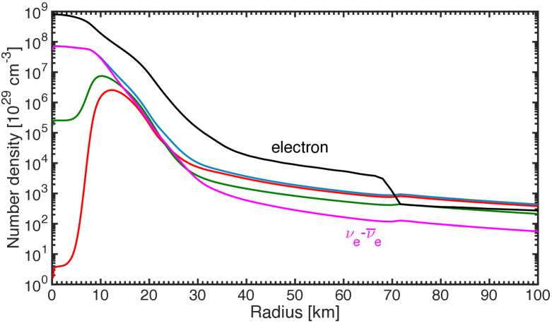
where $\Delta\mu_{ij}$ is the width of the $\mu=\cos\theta$ bin centered on $\mu_{ij}$ and the factor $2\pi$ arises from the azimuth integration $\int d\varphi$. The corresponding number flux density $\tilde{F}(r_{i})$ is the same expression with $\tilde{I}_{ijk}={I}_{ijk}/E_{k}$ under the sum. The overall neutrino luminosity of species $\nu_{\alpha}$ (${\rm MeV}~{}{\rm s}^{-1}$) at radial position $r_{i}$ is $L(r_{i})=4\pi r_{i}^{2}F(r_{i})$ and the analogous expression for the number luminosity or number flux (${\rm s}^{-1}$) is $\tilde{L}(r_{i})=4\pi r_{i}^{2}\tilde{F}(r_{i})$. The local neutrino number density (${\rm cm}^{-3}$) is

$$n(r_{i})=2\pi c^{-1}\sum_{k=1}^{N_{E}}\sum_{j=1}^{N_{\mu}}\Delta\mu_{ij}\tilde{I}_{ijk}\,.$$ (3)

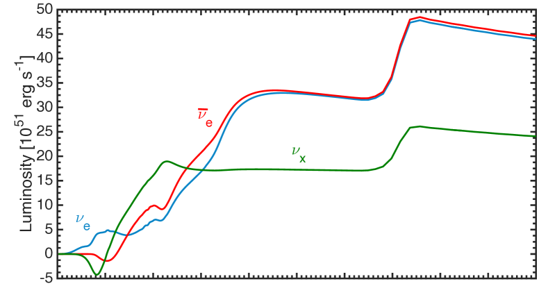
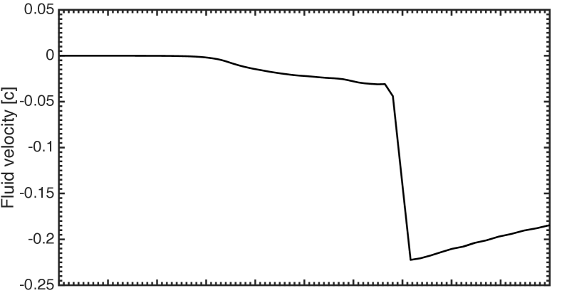
Figure 2 shows the radial variation of these and other characteristics, where quantities for $\nu_{e}$ are shown in blue, for $\bar{\nu}_{e}$ in red, and for $\nu_{x}$ in green. The upper left panel shows the flavor-dependent neutrino luminosities. Within the proto-neutron star, they show fast variations and are also negative in some region, indicating inward-flowing energy in agreement with the temperature profile shown in Fig. 3 which has a maximum at around 10 km. The radial variation depends strongly on flavor in agreement with the usual picture of flavor-dependent neutrino production and transport. The sudden increase at the shock-wave radius of around 75 km is an artifact of expressing the luminosities in the comoving fluid frame. The large infall velocity of around $-0.2\,c$ outside of the shock wave (upper right panel) introduces a significant blue shift of both the neutrino energies and their rate-of-flow. From the perspective of a distant observer in the laboratory frame, the luminosities remain continuous through the shock-wave region and are essentially constant beyond the decoupling region except for smaller changes (of the order of a few percent) due to energy deposition in the gain layer below the shock wave at around 75 km.

The $\nu_{x}$ flavor decouples at a smaller radius than $\nu_{e}$ and $\bar{\nu}_{e}$ and it reaches its shoulder in the luminosity profile at around 20 km. Also in this case, a further luminosity decline of a few percent (in the distant-observer frame) occurs from the energy transfer by inelastic neutrino-nucleon scattering of neutrinos on the cooler stellar plasma between the energy sphere and the transport sphere (Raffelt, 2001; Keil et al., 2003).

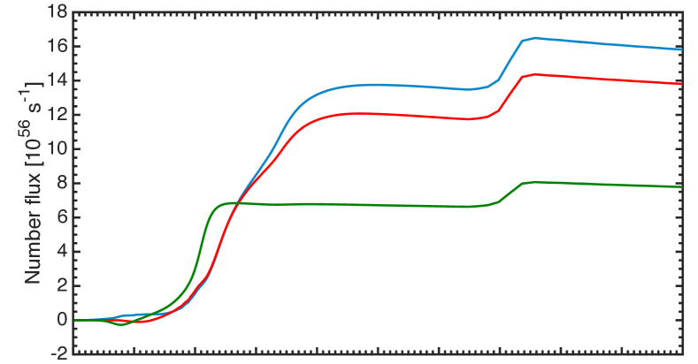
The neutrino number flux (or number luminosity) $\tilde{L}$ is shown in the left middle panel of Fig. 2. Qualitatively, its radial variation follows the luminosities. However, while the $\nu_{e}$ and $\bar{\nu}_{e}$ luminosities are nearly equal, the number fluxes differ by the $\nu_{e}$ deleptonization flux, compensated by lower average $\nu_{e}$ energies.

The local electron and neutrino number densities and the electron-neutrino lepton ($\nu_{e}-\bar{\nu}_{e}$) number density are shown in the lower left panel. From this plot one concludes that within the shock-wave radius all matter effects are certainly dominated by electrons, which, however, does not necessarily preclude neutrino self-induced flavor conversion.

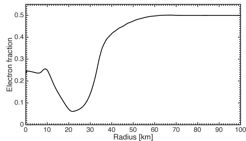
The electron fraction (bottom right panel) is locally defined as the ratio of the net electron number density to the proton plus neutron number density. Its profile reflects the deleptonization evolution of the infalling matter of the stellar core with the well-known trough around the neutrinospheric region and the continuous rise from the corresponding minimal value to the value of 0.5 (reached at 55 km) of the surrounding layers of the progenitor star.

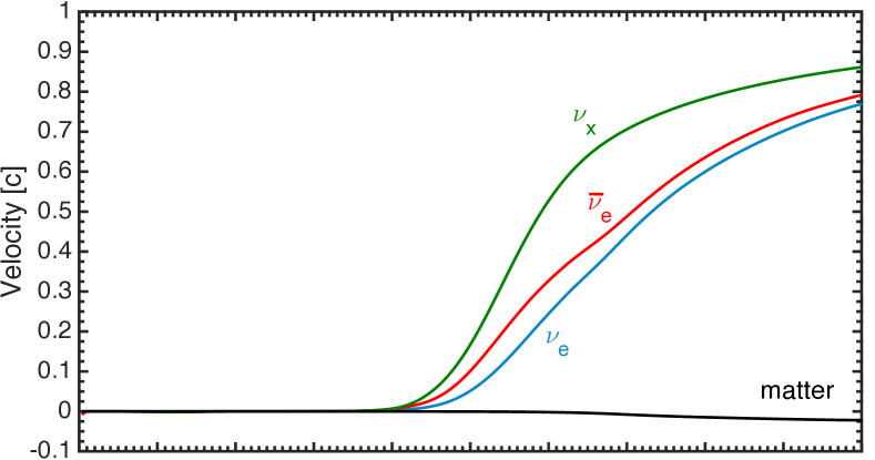
A quantity which nicely illustrates neutrino decoupling is the effective outward velocity of the neutrino fluid

$$v_{\rm eff}(r_{i})=\frac{\tilde{F}(r_{i})}{n(r_{i})}\,,$$ (4)

which is the number flux density divided by the number density. The ratio of $v_{\rm eff}$ to the speed of light, $f=v_{\rm eff}/c$ (displayed in the upper panel of Fig. 3), is often considered as the “flux factor” in neutrino-transport discussions. Figure 3 (upper panel) shows this quantity as a function of $r$ for the three species and also the fluid velocity of matter, which is the same as in the upper right panel of Fig. 2. Deep in the core, where the neutrino distribution is basically isotropic, $v_{\rm eff}$ is zero, whereas at large radii, where all neutrinos stream essentially in the radial direction with the speed of light, it approaches $c$. In agreement with Fig. 2, the decoupling happens in a flavor-dependent way and neutrinos start to decouple from the matter fluid at around 22 km. However, while $\nu_{x}$ decouple almost instantaneously, $\nu_{e}$ and $\bar{\nu}_{e}$ decouple over a much broader radial interval, in agreement with the upper left panel of Fig. 2.

Figure 3.— Radial variation of further properties of our benchmark model, supplementing Fig. 2 on a zoomed radial scale. Top panel: Effective neutrino velocity as defined in Eq. (4), normalized by the speed of light (“flux factor”), and the fluid velocity of the matter as in the upper-right panel of Fig. 2. Bottom panel: Local effective temperature of $\nu_{x}$ as defined in Eq. (5) and of the matter background.

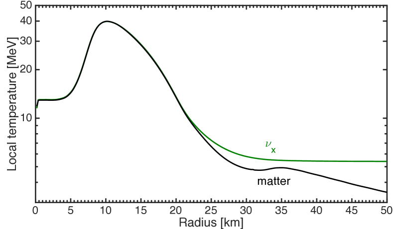
Another quantity that illustrates neutrino decoupling is the average neutrino energy at a given radius, where we mean the average $\langle E\rangle_{0}$ defined in Eq. (A9), which is the local neutrino energy density divided by the local number density without weighting with the angular projection factors $\mu$. For $\nu_{x}$ with vanishing chemical potential we define an effective temperature as

$$T(r_{i})=\frac{180\,\zeta_{3}}{7\pi^{4}}\,\langle E\rangle_{0}\simeq\frac{\sum_{k=1}^{N_{E}}\sum_{j=1}^{N_{\mu}}\Delta\mu_{ij}I_{ijk}}{3.15\sum_{k=1}^{N_{E}}\sum_{j=1}^{N_{\mu}}\Delta\mu_{ij}\tilde{I}_{ijk}}\,.$$ (5)

This quantity and the matter temperature are plotted in the bottom panel of Fig. 3. At $r\simeq 22$ km, the $\nu_{x}$ start to decouple from the stellar material and their temperature differs relative to the one of the surrounding matter. The effective $T$ of the final $\nu_{x}$ flux is considerably lower than it is at the “energy sphere” where $\nu_{x}$ begins to decouple; see Keil et al. (2003) for more details.

4. Angular variation of neutrino radiation field

In this section, we finally explore the neutrino angle distributions for all flavors, and in particular, how they vary with radius and evolve in time. We also observe that the local neutrino spectrum in a given direction of propagation is well described by a Gamma distribution.

4.1. Radial variation and temporal evolution of the neutrino angle distributions

In order to grasp the general trend of how the neutrino angular distributions vary in space and time we introduce at a given radius the local number intensity (see also Eq. A4),

$$\tilde{I}_{\mu}=2\pi\sum_{k=1}^{N_{E}}\tilde{I}_{ijk}\,,$$ (6)

which is the local number density of streaming neutrinos, integrated over energy and azimuth angle, but differential with regard to $\mu=\cos\theta$, and has units of ${\rm cm}^{-2}~{}{\rm s}^{-1}$. More specifically, in what follows, we will show the corresponding number density (not the number intensity), i.e., $\tilde{I}_{\mu}/c$, which has units ${\rm cm}^{-3}$.

Figure 4 shows $\tilde{I}_{\mu}/c$ for $\bar{\nu}_{e}$ as a function of $\theta$ for the indicated radial distances. The upper panel shows the distributions at small radii. As expected, inside the decoupling region the distribution is almost isotropic (see the magenta curve at $r=20$ km). At larger radii, the angle distributions become more and more forward peaked, corresponding to $\theta=0$. However, even at $r=37$ km (black curve), a non-negligible backward contribution remains clearly visible in this linear plot, confirming that neutrinos stream fully in the forward direction only for $r>40$ km, as speculated from Fig. 2. For $r=54$ km (blue curve), the distribution already becomes similar to a beam with a broad opening angle that becomes smaller with distance from the source, corresponding to the angular size of the SN core as seen from the given distance.

A logarithmic plot (bottom panel of Fig. 4), however, reveals that this picture is not complete. As neutrinos stream outward, they suffer residual collisions with the matter layers. As a consequence, the “neutrino beam” emerging from the source is accompanied by a “halo” which extends to all directions. The neutrino halo populating the large $\theta$ phase space is visible in the bottom panel of Fig. 4. One can see as the number intensity of the neutrino halo is small with respect to the neutrino beam propagating forward ($\theta\simeq 0$), but its broad angular distribution allows it to dominate the neutrino-neutrino interaction energy as discussed by Sarikas et al. (2012b).

Figure 4.— Number intensities for $\bar{\nu}_{e}$ as a function of zenith angle for the indicated radial distances of the 280 ms snapshot of our $15\,M_{\odot}$ model. Top: Linear plot for small radii. The angular distributions become more forward peaked for larger radii, but even at 37 km (black curve) they still stream in all directions. Bottom: Log-log-plot for larger radii, revealing the forward-peaked “neutrino beam” and a broad “halo” arising from residual scattering of the beam.

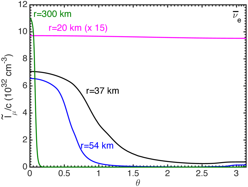
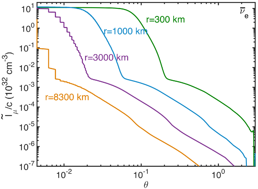
Figure 5 is a polar map of the normalized $\bar{\nu}_{e}$ monochromatic intensity $I_{E,\Omega}$ introduced in Eq. (1) for $E_{k}=10$ MeV and at different radii. For larger radii, the distributions become more forward peaked, and outside of the neutrino-decoupling region the intensity is essentially conserved along radiation paths that point outward from the radiating neutrinosphere. A similar behavior was also found by Thompson et al. (2003), see their Figs. 4 and 10–12.

Figure 5.— Radial variation of the normalized spectral intensity $I_{E,\Omega}$ of $\bar{\nu}_{e}$ for $E=10$ MeV and the 280 ms snapshot of our $15\,M_{\odot}$ model as a function of the zenith direction angle. The angle $\theta=0$ refers to the local radial direction.

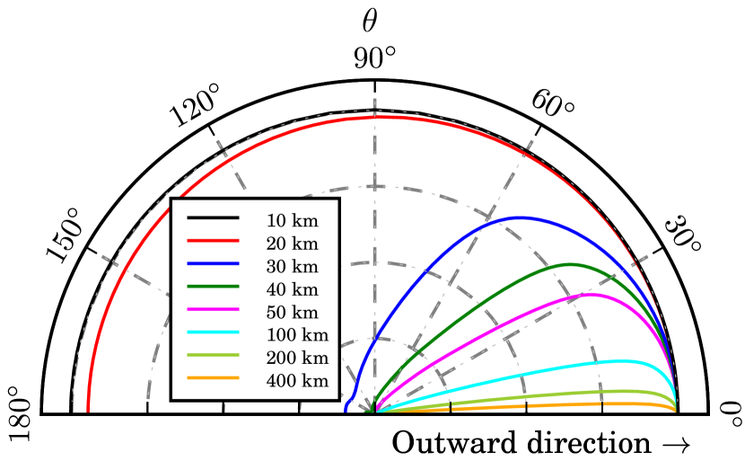
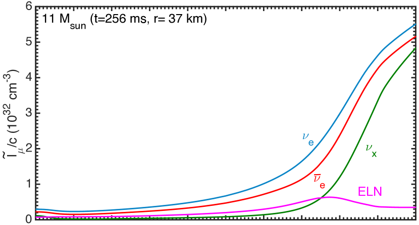
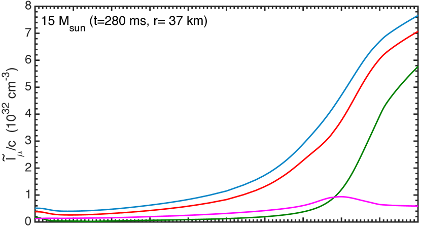
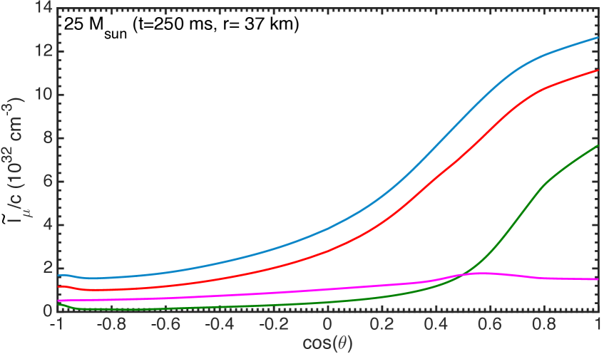
Figure 6 shows the flavor dependent angle distributions for our three progenitors. The width of the distributions decreases in the sequence $\nu_{e}$, $\bar{\nu}_{e}$ and $\nu_{x}$ (Ott et al., 2008; Sarikas et al., 2012a) as expected from the decreasing interaction rates in the medium. Qualitatively, this behavior is the same for all progenitors. At some radii, the angular distributions of $\nu_{e}$ and $\nu_{x}$ or the ones of $\bar{\nu}_{e}$ and $\bar{\nu}_{x}$ may cross as assumed in Mirizzi & Serpico (2012).

Figure 6.— Neutrino number intensity as a function of $\cos\theta$ for the species $\nu_{e}$ in blue, $\bar{\nu}_{e}$ in red, $\nu_{x}$ in green, and $\nu_{e}-\bar{\nu}_{e}$ in magenta as indicated. From top to bottom for snapshots at comparable times at 37 km for our three progenitor models as indicated in the panels. As expected, the height and width of the distributions decreases in the sequence $\nu_{e}$, $\bar{\nu}_{e}$ and $\nu_{x}$.

4.2. Neutrino electron lepton number

A new issue in the context of self-induced neutrino flavor conversion is the question of the angular distribution of the electron lepton number (ELN) carried by neutrinos and in particular the question of possible crossings of the $\bar{\nu}_{e}$ with the $\nu_{e}$ angle distributions (Sawyer, 2016; Izaguirre et al., 2017). Such situations could trigger fast flavor conversion, i.e., self-induced flavor conversion where the instability scale is not set by the neutrino mass differences, but rather by the neutrino-neutrino interaction energy, a much larger scale for typical SN conditions.

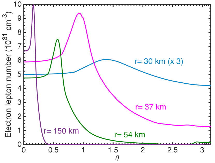
The ELN carried by neutrinos, defined as $(\tilde{I}_{\mu,\nu_{e}}-\tilde{I}_{\mu,\bar{\nu}_{e}})/c$, is shown in magenta in Fig. 6 for the selected snapshots of our three progenitors. It is comparable in intensity for all three progenitors, but the dip in the forward direction is less pronounced for the $25\,M_{\odot}$ SN model for the selected post-bounce time and radius. Figure 7 shows the ELN as a function of $\theta$ for different radii for our benchmark model. It develops a dip in the forward direction as the radius increases. We also provide an animation of the ELN variation with radius for the $15\,M_{\odot}$ progenitor here. In all of our models we have found the ELN to be always positive. In particular, the universal dip in the forward direction never turns negative, so there is no crossing between the $\nu_{e}$ and $\bar{\nu}_{e}$ angular distributions. On the contrary, crossings in the ELN distribution naturally appear in compact merger remnants because of the different emission geometry with respect to SNe and the $\bar{\nu}_{e}$ flux being larger than the $\nu_{e}$ one (Wu & Tamborra, 2017).

Figure 7.— Angular distribution of the neutrino electron lepton number for the 280 ms snapshot of the $15\,M_{\odot}$ progenitor extracted at different radii as indicated.

This behavior could change in 3D models, for example in the presence of LESA (Lepton-Emission Self-sustained Asymmetry; Tamborra et al., 2014a). LESA manifests itself in a pronounced large-scale dipolar pattern in the ELN emission. This is a consequence of large-scale convection modes inside the newly formed neutron star with a strong dipolar flow component, which grows during the contraction phase (Janka et al., 2016) and has significant feedback also on the accretion flow around the neutron star (Tamborra et al., 2014a). LESA naturally implies a change of sign in $(\tilde{I}_{\mu,\nu_{e}}-\tilde{I}_{\mu,\bar{\nu}_{e}})$. It is therefore conceivable that, especially in the regions where the ELN changes its sign, crossings in the ELN angular distributions may occur.

Existing 3D simulations employ, however, the ray-by-ray transport approximation (Melson et al., 2015b, a; Lentz et al., 2015; Takiwaki et al., 2014) or multi-dimensional two-moment treatments with algebraic closure relations such as the “M1 methods” Roberts et al. (2016). None of these can provide reliable angle distributions. M1 solvers use the neutrino energy and momentum equations to evolve the angle-integrated moments of the neutrino intensity (i.e., the energy-dependent energy and flux densities). The ray-by-ray approximation, even if based on a two-moment solver with Boltzmann closure (Rampp & Janka, 2002; Buras et al., 2006), makes use of the assumption that the neutrino intensity is locally axially symmetric around the radial direction. It thus ignores non-radial flux components and off-diagonal elements in the pressure tensor. For certain questions (e.g. for rough estimates of observable emission asymmetries) one can work around the missing phase-space information by using low-order multipole approximations of the intensity based on energy-density and flux-density information (Müller et al., 2012; Tamborra et al., 2014b). Detailed, accurate phase-space information, however, requires the solution of the time-dependent Boltzmann transport equation for the neutrino intensity in dependence on all three spatial and all three momentum-space variables.

Existing supercomputers can hardly tackle this high-dimensional problem in two spatial dimensions despite severe restrictions with respect to resolution and sophistication of the employed weak-interaction physics (Ott et al., 2008; Brandt et al., 2011; Nagakura et al., 2017). Time-dependent numerical solutions of the Boltzmann transport equation in 3D will require exascale computing capability, but will still be very challenging when high resolution in momentum space is required. The results based on a tangent-ray integration of the energy and angle-dependent Boltzmann equation in 1D presented in this work are therefore likely to set the benchmark for neutrino-oscillation studies for the coming years.

4.3. Spectral fit

Figure 8.— Representative example for the $\bar{\nu}_{e}$ spectrum (energy distribution) at $r=30$ km for the 280 ms snapshot of the $15\,M_{\odot}$ model, where blue is for $\cos(\theta)=1$ and red for $\cos(\theta)=-0.9$. Top panel: Normalized histogram of the numerical spectrum and fit by a Gamma distribution (smooth line). Bottom panel: Same fit (blue line) as well as a similar fit for a nearly backward direction, both of them normalized to the same value at maximum. The backward flux has larger energies caused by the energy dependence of the neutrino cross sections.

Flavor oscillation effects generally depend both on neutrino energy and angle. Therefore, in our data files we also provide information about the energy distribution. It has been observed previously that SN neutrino energy spectra often can be well approximated by a Gamma distribution  (Keil et al., 2003; Tamborra et al., 2012), sometimes also referred to as “$\alpha$ fit.” In our context it means that we will express the spectral intensities in the form

$$I_{E,\theta}\propto\left(\frac{E}{E_{\theta}}\right)^{\alpha_{\theta}}e^{-(\alpha_{\theta}+1)E/E_{\theta}}\,,$$ (7)

where the energy $E_{\theta}=\langle E\rangle_{\theta}$ is the average energy of the neutrinos streaming in direction $\theta$, whereas the shape parameter $\alpha_{\theta}$ measures the amount of spectral pinching. It is related to the first and second energy moments through

$$\frac{\langle E^{2}\rangle_{\theta}}{\langle E\rangle_{\theta}^{2}}=\frac{2+\alpha_{\theta}}{1+\alpha_{\theta}}\,.$$ (8)

Besides the energy-integrated intensity $I_{\mu}$ we provide the first two energy moments (Eqs. B2, B3) for any $\mu$ and in this way characterize the spectra with reasonable accuracy.

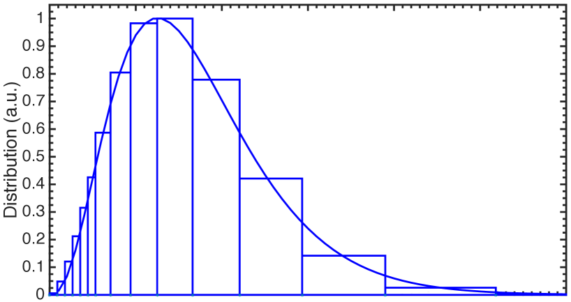
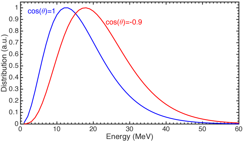
As a representative example, we show in Fig. 8 the $\bar{\nu}_{e}$ energy spectrum at $r=30$ km for our benchmark SN model. We consider the outward direction ($\mu=1$ in blue) and a nearly backward direction ($\mu=-0.9$ in red). For the former we show both the numerical distribution as a histogram and the fit by a Gamma distribution (top panel). We then compare the smooth fits for both directions (bottom panel of Fig. 8), illustrating that the energy distributions depend significantly on direction simply because of the energy-dependent neutrino scattering cross sections. A similar comparison was provided by Sarikas et al. (2012b) at large distances to compare the spectrum of the neutrinos coming directly from the SN core vs. the halo flux which arises from residual scattering. In our case, we find that the $\bar{\nu}_{e}$ streaming in the forward direction have $E_{\theta}=17.1$ MeV and $\alpha_{\theta}=2.7$ and are therefore cooler and less pinched than the quasi-backward direction, where $E_{\theta}=22.1$ MeV and $\alpha_{\theta}=4$. More energetic neutrinos are typically more isotropically distributed in energy than less energetic ones.

5. Conclusions

Recent developments in the context of neutrino-neutrino interactions in dense media have highlighted the role of the neutrino angular distributions. For the first time, we have carried out a careful analysis of the neutrino angular distributions from one-dimensional hydrodynamical SN simulations with sophisticated neutrino transport.

To facilitate dedicated studies of flavor conversion, we provide data of the energy and angle distributions as supplementary material. We specifically explore the angle distributions of neutrinos in three SN progenitors with masses of 11.2, 15 and $25\,M_{\odot}$, and scan three different post-bounce times during the accretion phase for each of them.

The neutrino radiation field ranges from being completely isotropic inside the proto-neutron star, where neutrinos frequently scatter, to being forward peaked at large distances from the proto-neutron star (50 km for the analyzed models) where neutrinos stream almost freely. However, while propagating further, neutrinos scatter on nuclei in the stellar envelope, generating a broad “halo” and backward distribution, becoming relevant at larger radii. The neutrino radiation flowing in the backward direction is in general characterized by an energy spectrum hotter and more pinched than the forward streaming component.

The question if fast flavor conversion occurs in the neutrino decoupling region will require a better theoretical understanding of the behavior of the neutrino radiation field in the SN environment. Our present study provides the input information that is required for such studies.

Appendix A Neutrino Radiation Field

In the context of neutrino flavor oscillation studies, the local neutrino radiation field for a given species $\nu_{e}$, $\bar{\nu}_{e}$ or $\nu_{x}$ is traditionally described by occupation numbers (classical phase-space densities) $f({\bf p})$ for every momentum mode ${\bf p}$. These can be extended to $3{\times}3$ matrices $\varrho({\bf p})$ to capture flavor coherence on the off-diagonal elements. On the other hand, in the traditional treatment of neutrino radiative transfer, one uses the spectral intensity $I_{E,\Omega}$ as the fundamental quantity, i.e., the energy carried by the given neutrino species per unit area and unit time, differential with respect to neutrino energy $E$ and solid angle $\Omega$ (see Eq. 1). Moreover, in the particle-physics tradition one uses natural units with $\hbar=c=1$, although we will keep $\hbar$ and $c$ explicitly here. In this appendix, we provide a brief dictionary between these languages because simple issues of definition, normalization or units can be a source of confusion.

Taking neutrinos to be massless, their energy is $E=c|{\bf p}|$. Therefore, the differential local number density is

$$dn=\frac{f_{\bf p}}{\hbar^{3}}\,\frac{d^{3}{\bf p}}{(2\pi)^{3}}=\frac{f_{E,\Omega}}{(\hbar c)^{3}}\,\frac{E^{2}dEd\Omega}{(2\pi)^{3}}\,,$$ (A1)

where we show the dependence on ${\bf p}$, $E$, or $\Omega$ as indices. In the second expression the neutrino momentum is represented by its energy and direction of motion. Noting that massless neutrinos stream with the speed of light $c$ in a given direction $\Omega$, the spectral intensity is

$$I_{E,\Omega}=cE\,\frac{dn}{dEd\Omega}=\frac{f_{E,\Omega}}{\hbar^{3}c^{2}}\,\frac{E^{3}}{(2\pi)^{3}}$$ (A2)

in units of ${\rm cm}^{-2}~{}{\rm s}^{-1}~{}{\rm ster}^{-1}$. Integrating over all energies, the intensity is $I_{\Omega}=\int_{0}^{\infty}I_{E,\Omega}\,dE$ in units of ${\rm MeV}~{}{\rm cm}^{-2}~{}{\rm s}^{-1}~{}{\rm ster}^{-1}$.

In the neutrino flavor evolution context, the relevant quantities are number densities and number fluxes, not energy densities or fluxes. To develop a systematic notation we here use a tilde on a symbol for the corresponding number quantity. In particular, we define the spectral number intensity

$$\tilde{I}_{E,\Omega}=\frac{I_{E,\Omega}}{E}=c\,\frac{dn}{dEd\Omega}=\frac{f_{E,\Omega}}{\hbar^{3}c^{2}}\,\frac{E^{2}}{(2\pi)^{3}}$$ (A3)

in units of ${\rm cm}^{-2}~{}{\rm s}^{-1}~{}{\rm MeV}^{-1}~{}{\rm ster}^{-1}$.

For producing a weak potential on other neutrinos, a more intuitive quantity is the local number density, differential with regard to energy and solid angle. Therefore, without introducing a special symbol, our real quantity of interest is $\tilde{I}_{E,\Omega}/c$ in units of ${\rm cm}^{-3}~{}{\rm MeV}^{-1}~{}{\rm ster}^{-1}$. Of course, in natural units where $c=1$, both quantities are the same. Still, there is a conceptual difference between a flux-like quantity ($I_{E,\Omega}$ or $\tilde{I}_{E,\Omega}$) and a density, even though for relativistic particles they are equivalent except for units.

Henceforth we assume that the radiation field is axially symmetric around the local radial direction. Moreover, we assume that the overall SN model is spherically symmetric. We use local polar coordinates $\Omega=(\theta,\varphi)$ with the differential $d\Omega=d\mu\,d\varphi$ with $\mu=\cos\theta$. The azimuthal integration $\int d\varphi\to 2\pi$ is trivial because of the assumed symmetry.

In particular, we are interested in the number intensity, integrated over energy and azimuth angle, which is

$$\frac{\tilde{I}_{\mu}}{c}=\int dE\,d\varphi\frac{\tilde{I}_{E,\Omega}}{c}=\int dE\frac{f_{E,\mu}}{(\hbar c)^{3}}\,\frac{E^{2}}{(2\pi)^{2}}$$ (A4)

in units of ${\rm cm}^{-3}$, a quantity which remains differential with regard to $\mu$. Integrating it over $d\mu$ gives us the local number density $n$ of the given neutrino species.

We define the local specific flux density (of energy) in the radial direction in the form

$$F_{E}=\int d\Omega\,\mu\,I_{E,\Omega}=\int d\Omega\,\mu\,\frac{f_{E,\Omega}}{\hbar^{3}c^{2}}\,\frac{E^{3}}{(2\pi)^{3}}$$ (A5)

in units of ${\rm cm}^{-2}~{}{\rm s}^{-1}$. The corresponding energy flux density is

$$F=\int dE\,d\Omega\,\mu\,I_{E,\Omega}=\int dE\,d\Omega\,\mu\,\frac{f_{E,\Omega}}{\hbar^{3}c^{2}}\,\frac{E^{3}}{(2\pi)^{3}}$$ (A6)

in units of ${\rm MeV}~{}{\rm cm}^{-2}~{}{\rm s}^{-1}$. Finally, the luminosity of the entire SN at a given radius $r$ is

$$L=4\pi r^{2}F=4\pi r^{2}\int dE\,d\Omega\,\mu\,I_{E,\Omega}$$ (A7)

in units of ${\rm MeV}~{}{\rm s}^{-1}$. The corresponding number-quantities (symbols with tildes) are the same expressions with $E^{-1}$ under the integrals. In particular, $\tilde{L}$, the “number luminosity,” is the total number of neutrinos per second of the given species streaming outward through a surface of radius $r$.

At large distances from the SN, we usually define the average neutrino energy in the form

$$\langle E\rangle=\frac{F}{\widetilde{F}}=\frac{\int dE\,d\Omega\,\mu\,\frac{f_{E,\Omega}}{\hbar^{3}c^{2}}\,\frac{E^{3}}{(2\pi)^{3}}}{\int dE\,d\Omega\,\mu\,\frac{f_{E,\Omega}}{\hbar^{3}c^{2}}\,\frac{E^{2}}{(2\pi)^{3}}}\,,$$ (A8)

which is the average energy of the neutrino flux at distance $r$. In deeper regions around and below the weak decoupling region, we may also consider the local average energy, without weighting it with the angular projection factor $\mu$, so

$$\langle E\rangle_{0}=\frac{\int dE\,d\Omega\,\frac{f_{E,\Omega}}{\hbar^{3}c^{2}}\,\frac{E^{3}}{(2\pi)^{3}}}{\int dE\,d\Omega\,\frac{f_{E,\Omega}}{\hbar^{3}c^{2}}\,\frac{E^{2}}{(2\pi)^{3}}}\,.$$ (A9)

It is this quantity which we have shown in Fig. 3 as temperature ($T_{0}=\langle E\rangle_{0}/3.15$).

Appendix B Data Structure

The quantity provided by SN simulations is the monochromatic neutrino intensity for each flavor $\nu_{\alpha}$, integrated over the energy bin centered on $E_{k}$, for each radial point $r_{i}$ and zenith-angle $\mu_{ij}$. Those data can be downloaded from the Garching SN Archive upon request.

We here provide data useful for neutrino oscillation studies for three progenitors and three selected post-bounce times as supplementary material and give brief instructions on how to read the data files. All data refer to quantities in a coordinate frame that moves with the matter fluid.

The files named as “radial-neutrino-properties-time-SNmass.dat” list the angle-integrated neutrino emission properties as a function of the radius ($r_{i}$). The first column lists the radius. The luminosities $L(r_{i})$ of $\nu_{e}$, $\bar{\nu}_{e}$ and $\nu_{x}$ are stored in the second, third, and fourth columns, respectively. The first energy moments, defined as in Eq. (A8), for $\nu_{e}$, $\bar{\nu}_{e}$ and $\nu_{x}$ are stored in the fifth, sixth and seventh columns. The second energy moments for these flavors are stored in the eighth, ninth and tenth columns. By using these data and Eq. (7) one can reconstruct the variation of the neutrino energy spectra in the SN comoving frame as a function of the distance from the proto-neutron star radius.

The files named as “angular-quantities-nualpha-time-SNmass.dat” list the angle- and radius-dependent neutrino emission properties for each flavor $\nu_{\alpha}$ and for each selected post-bounce time and progenitor mass. The radius $r_{i}$ is listed in the first column, $\mu_{ij}$ is reported in the second column. Note that the binning in $\mu_{ij}$ is not uniform as a function of $r_{i}$ because of the tangent-ray discretization of the Boltzmann transport equation (see Rampp & Janka (2002) for more details). Moreover, degenerate angular zones of measure zero may be present around $\theta=\pi/2$ due to the peculiar angular-grid formulation.

The third column of the file “angular-quantities-nualpha-time-SNmass.dat” lists the differential (with respect to $\mu$, i.e., per unit interval of the cosine of the zenith angle) neutrino number luminosity (0-th moment, in units of s^-1) defined as

$$\tilde{L}_{\mu}(r_{i},\mu_{ij})=4\pi r_{i}^{2}\sum_{k=1}^{N_{E}}2\pi\tilde{I}_{ijk}\ .$$ (B1)

We recover the neutrino number luminosity $\tilde{L}(r_{i})$ by integrating the equation above over $\mu_{ij}$. The fourth column represents the first energy moment (in units of MeV s^-1):

$$L_{\mu}(r_{i},\mu_{ij})=4\pi r_{i}^{2}\sum_{k=1}^{N_{E}}2\pi I_{ijk}\ ,$$ (B2)

while the second energy moment (in units of MeV² s^-1) is reported in fifth column and it is defined as

$$S_{\mu}(r_{i},\mu_{ij})=4\pi r_{i}^{2}\sum_{k=1}^{N_{E}}2\pi I_{ijk}E_{k}\ .$$ (B3)

The differential neutrino density is stored in the sixth column (in units of cm^-3) and it is defined as

$$\frac{\tilde{I}_{\mu}(r_{i},\mu_{ij})}{c}=2\pi c^{-1}\sum_{k=1}^{N_{E}}\tilde{I}_{ijk}\ .$$ (B4)

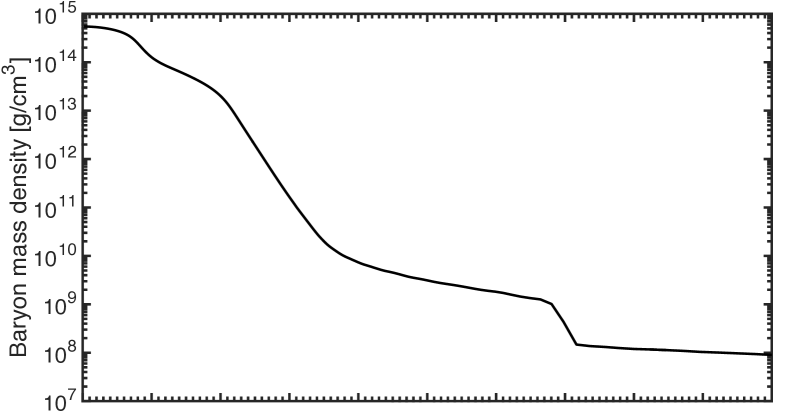
For all SN models, we used 21 nearly geometrically spaced energy bins up to 380 MeV and a number tangent rays and radial grid points that vary as functions of post-bounce time: $N_{\mu}=510,N_{r}=235$ for $t=61$ ms, $N_{\mu}=836,N_{r}=398$ for $t=256$ ms and $N_{\mu}=838,N_{r}=399$ for $t=550$ ms for the $11.2M_{\odot}$ model; $N_{\mu}=672,N_{r}=316$ for $t=150$ ms, $N_{\mu}=824,N_{r}=392$ for $t=280$ ms and $N_{\mu}=914,N_{r}=437$ for $t=500$ ms for the $15M_{\odot}$ SN progenitor; $N_{\mu}=510,N_{r}=235$ for $t=63$ ms, $N_{\mu}=780,N_{r}=370$ for $t=252$ ms and $N_{\mu}=784,N_{r}=372$ for $t=352$ ms for the $25M_{\odot}$ SN progenitor. For all studied progenitors and post-bounce times, we also provide data on the matter density profile, the electron abundance, the velocity profile, central and boundary values of the energy bins, and the radial grid.

References

- Brandt et al. (2011) Brandt, T. D., Burrows, A., Ott, C. D., & Livne, E. 2011, Astrophys. J., 728, 8
- Buras et al. (2003) Buras, R., Janka, H.-T., Keil, M. T., Raffelt, G. G., & Rampp, M. 2003, ApJ, 587, 320
- Buras et al. (2006) Buras, R., Rampp, M., Janka, H.-T., & Kifonidis, K. 2006, A&A, 447, 1049
- Burrows (2013) Burrows, A. 2013, Rev. Mod. Phys., 85, 245
- Chakraborty et al. (2016a) Chakraborty, S., Hansen, R., Izaguirre, I., & Raffelt, G. G. 2016a, Nucl. Phys. B, 908, 366
- Chakraborty et al. (2016b) Chakraborty, S., Hansen, R. S., Izaguirre, I., & Raffelt, G. G. 2016b, JCAP, 1603, 042
- Cherry et al. (2012) Cherry, J. F., Carlson, J., Friedland, A., Fuller, G. M., & Vlasenko, A. 2012, Phys. Rev. Lett., 108, 261104
- Dasgupta et al. (2017) Dasgupta, B., Mirizzi, A., & Sen, M. 2017, JCAP, 1702, 019
- Dimmelmeier et al. (2002) Dimmelmeier, H., Font, J. A., & Müller, E. 2002, A&A, 388, 917
- Duan et al. (2006) Duan, H., Fuller, G. M., Carlson, J., & Qian, Y.-Z. 2006, Phys. Rev. D, 74, 105014
- Duan et al. (2010) Duan, H., Fuller, G. M., & Qian, Y.-Z. 2010, Ann. Rev. Nucl. Part. Sci., 60, 569
- Hüdepohl (2013) Hüdepohl, L. 2013, PhD thesis, Technische Universität München
- Hüdepohl et al. (2010) Hüdepohl, L., Müller, B., Janka, H.-T., Marek, A., & Raffelt, G. G. 2010, Phys. Rev. Lett., 104, 251101, [Erratum: Phys. Rev. Lett. 105,249901(2010)]
- Izaguirre et al. (2017) Izaguirre, I., Raffelt, G. G., & Tamborra, I. 2017, Phys. Rev. Lett., 118, 021101
- Janka (2012) Janka, H.-T. 2012, Ann. Rev. Nucl. Part. Sci., 62, 407
- Janka et al. (2012) Janka, H.-T., Hanke, F., Hüdepohl, L., Marek, A., Müller, B., & Obergaulinger, M. 2012, PTEP, 2012, 01A309
- Janka et al. (2016) Janka, H. T., Melson, T., & Summa, A. 2016, Ann. Rev. Nucl. Part. Sci., 66, 341
- Keil et al. (2003) Keil, M. T., Raffelt, G. G., & Janka, H.-T. 2003, ApJ, 590, 971
- Langanke et al. (2008) Langanke, K., Martínez-Pinedo, G., Müller, B., Janka, H.-T., Marek, A., Hix, W. R., Juodagalvis, A., & Sampaio, J. M. 2008, Phys. Rev. Lett., 100, 011101
- Langanke et al. (2003) Langanke, K., Martínez-Pinedo, G., Sampaio, J. M., Dean, D. J., Hix, W. R., Messer, O. E., Mezzacappa, A., Liebendörfer, M., Janka, H.-T., & Rampp, M. 2003, Phys. Rev. Lett., 90, 241102
- Lattimer & Swesty (1991) Lattimer, J. M. & Swesty, F. D. 1991, Nucl. Phys., A535, 331
- Lentz et al. (2015) Lentz, E. J., Bruenn, S. W., Hix, W. R., Mezzacappa, A., Messer, O. E. B., Endeve, E., Blondin, J. M., Harris, J. A., Marronetti, P., & Yakunin, K. N. 2015, ApJ, 807, L31
- Liebendörfer et al. (2005) Liebendörfer, M., Rampp, M., Janka, H.-T., & Mezzacappa, A. 2005, ApJ, 620, 840
- Marek et al. (2006) Marek, A., Dimmelmeier, H., Janka, H.-T., Müller, E., & Buras, R. 2006, A&A, 445, 273
- Melson et al. (2015a) Melson, T., Janka, H.-T., Bollig, R., Hanke, F., Marek, A., & Müller, B. 2015a, Astrophys. J., 808, L42
- Melson et al. (2015b) Melson, T., Janka, H.-T., & Marek, A. 2015b, Astrophys. J., 801, L24
- Mirizzi & Serpico (2012) Mirizzi, A. & Serpico, P. D. 2012, Phys. Rev. Lett., 108, 231102
- Mirizzi et al. (2016) Mirizzi, A., Tamborra, I., Janka, H.-T., Saviano, N., Scholberg, K., Bollig, R., Hüdepohl, L., & Chakraborty, S. 2016, Riv. Nuovo Cim., 39, 1
- Müller et al. (2010) Müller, B., Janka, H.-T., & Dimmelmeier, H. 2010, ApJS, 189, 104
- Müller et al. (2012) Müller, E., Janka, H. T., & Wongwathanarat, A. 2012, Astron. Astrophys., 537, A63
- Nagakura et al. (2017) Nagakura, H., Iwakami, W., Furusawa, S., Okawa, H., Harada, A., Sumiyoshi, K., Yamada, S., Matsufuru, H., & Imakura, A. 2017
- Ott et al. (2008) Ott, C. D., Burrows, A., Dessart, L., & Livne, E. 2008, Astrophys. J., 685, 1069
- Raffelt (2001) Raffelt, G. G. 2001, ApJ, 561, 890
- Rampp & Janka (2002) Rampp, M. & Janka, H.-T. 2002, A&A, 396, 361
- Roberts et al. (2016) Roberts, L. F., Ott, C. D., Haas, R., O’Connor, E. P., Diener, P., & Schnetter, E. 2016
- Sarikas et al. (2012a) Sarikas, S., Raffelt, G. G., Hüdepohl, L., & Janka, H.-T. 2012a, Phys. Rev. Lett., 108, 061101
- Sarikas et al. (2012b) Sarikas, S., Tamborra, I., Raffelt, G. G., Hüdepohl, L., & Janka, H.-T. 2012b, Phys. Rev. D, 85, 113007
- Sawyer (2005) Sawyer, R. F. 2005, Phys. Rev. D, 72, 045003
- Sawyer (2009) —. 2009, Phys. Rev. D, 79, 105003
- Sawyer (2016) —. 2016, Phys. Rev. Lett., 116, 081101
- Scholberg (2012) Scholberg, K. 2012, Ann. Rev. Nucl. Part. Sci., 62, 81
- Sumiyoshi et al. (2015) Sumiyoshi, K., Takiwaki, T., Matsufuru, H., & Yamada, S. 2015, Astrophys. J. Suppl., 216, 5
- Takiwaki et al. (2014) Takiwaki, T., Kotake, K., & Suwa, Y. 2014, Astrophys. J., 786, 83
- Tamborra et al. (2014a) Tamborra, I., Hanke, F., Janka, H.-T., Müller, B., Raffelt, G. G., & Marek, A. 2014a, ApJ, 792, 96
- Tamborra et al. (2012) Tamborra, I., Müller, B., Hüdepohl, L., Janka, H.-T., & Raffelt, G. G. 2012, Phys. Rev. D, 86, 125031
- Tamborra et al. (2014b) Tamborra, I., Raffelt, G., Hanke, F., Janka, H.-T., & Müller, B. 2014b, Phys. Rev., D90, 045032
- Thompson et al. (2003) Thompson, T. A., Burrows, A., & Pinto, P. A. 2003, ApJ, 592, 434
- Woosley et al. (2002) Woosley, S. E., Heger, A., & Weaver, T. A. 2002, Rev. Mod. Phys., 74, 1015
- Woosley & Weaver (1995) Woosley, S. E. & Weaver, T. A. 1995, ApJ Suppl., 101, 181
- Wu & Tamborra (2017) Wu, M.-R. & Tamborra, I. 2017, arXiv:1701.06580 [astro-ph.HE]