NIMROD Modeling of Quiescent H-mode: Reconstruction Considerations and Saturation Mechanism

Abstract

The extended-MHD NIMROD code [C.R. Sovinec and J.R. King, J. Comput. Phys. 229, 5803 (2010)] models broadband-MHD activity from a reconstruction of a quiescent H-mode shot on the DIII-D tokamak [J. L. Luxon, Nucl. Fusion 42, 614 (2002)]. Computations with the reconstructed toroidal and poloidal ion flows exhibit low-$n_{\phi}$ perturbations ($n_{\phi}\simeq 1-5$) that grow and saturate into a turbulent-like MHD state. The workflow used to project the reconstructed state onto the NIMROD basis functions re-solves the Grad-Shafranov equation and extrapolates profiles to include scrape-off-layer currents. Evaluation of the transport from the turbulent-like MHD state leads to a relaxation of the density and temperature profiles. Published version: Nucl. Fusion 57 022002 (2017) [http://dx.doi.org/10.1088/0029-5515/57/2/022002]

I Introduction

It is desirable to have an ITER ITER Physics Basis Editors (1999) H-mode regime that is quiescent to edge-localized modes (ELMs) Connor et al. (1998); Leonard et al. (2006). ELMs deposit large, localized and impulsive heat loads that can damage the divertor. A quiescent regime with edge harmonic oscillations (EHO) or broadband MHD activity is observed in some DIII-D Burrell et al. (2001, 2005, 2009); Garofalo et al. (2011); Burrell et al. (2012, 2013); Solomon et al. (2014); Garofalo et al. (2015), JT-60U Sakamoto et al. (2004); Oyama et al. (2005), JET Solano et al. (2010) and ASDEX-U Suttrop et al. (2005), discharge scenarios. These ELM-free discharges have the pedestal-plasma confinement necessary for burning-plasma operation in ITERGarofalo et al. (2015). The mode activity associated with the EHO or broadband MHD on DIII-D is characterized by small toroidal-mode numbers ($n_{\phi}\simeq 1-5$) and is thus suitable for simulation with global MHD codes. Measurements from beam-emission spectroscopy, electron-cyclotron emission, and magnetic probe diagnostics show highly coherent density, temperature and magnetic oscillations associated with EHO. The particle and impurity Grierson et al. (2015) transport is enhanced during QH-mode, leading to essentially steady-state profiles in the pedestal region.

Relative to QH-mode operation with EHO, operation with broadband MHD tends to occur at higher densities and lower rotation and thus may be more relevant to potential ITER discharge scenarios. While there are computational investigations of the discharges with EHO Liu et al. (2015); Battaglia et al. (2014), there is less computational analysis of discharges with broadband MHD. In this paper, we investigate the broadband-MHD state with nonlinear NIMROD Sovinec et al. (2004); Sovinec and King (2010) simulations initialized from a reconstruction of a DIII-D QH-mode discharge with broadband MHD. These simulations include the reconstructed flow and saturate into a turbulent-like state.

This paper is organized as follows. As an initial-value computation, our simulations require accurate and smooth initial conditions to avoid spurious instabilities. Section II describes how the reconstructed fields are imported into the NIMROD spatial discretization. One of the novel methods in our approach to this edge modeling is to extrapolate the pressure and density profiles through the scrape-off layer (SOL) to maintain first-order continuity and thus a continuous current profile when solving the Grad-Shafranov equation. The section concludes by discussing our assumptions where the reconstructed fields are in steady state, and how our modeling simulates the dynamics of perturbations about this steady state. In Sec. III, the model equations and the dynamics of our nonlinear MHD simulations that saturate into a turbulent-like state are considered. The magnetic stochasticity and transport induced from these perturbations are analyzed in Sec. IV. Finally, we conclude with a discussion of the implications and limitations of our present modeling and mention future directions for this work.

II Extended equilibrium reconstruction for NIMROD

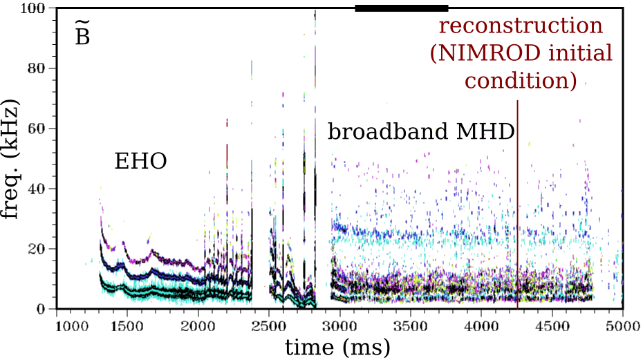
Figure 1: [Color online] Cross-power spectrum plot of the magnetic fluctuation probe measurements from DIII-D shot 145098. An initial phase contains coherent EHO fluctuations followed by a phase with broadband-MHD activity. The NIMROD simulation is initialized from a reconstruction during the latter phase at 4250 ms.

The cross-power spectrum from magnetic fluctuation probe measurements on DIII-D during shot 145098 is shown in Fig. 1. This shot is part of a campaign to create a QH-mode discharge with ITER-relevant parameters and shape, the ultimate results of which are summarized in Ref. Garofalo et al. (2015). As the torque is ramped down the mode activity transitions from EHO to broadband MHD. An EFIT Lao et al. (1985, 2005) reconstruction, constrained by magnetic-probe, motional-stark-effect, Thomson-scattering, and charge-exchange-recombination (CER) measurements, is used to specify the initial condition in the NIMROD code. High quality equilibria are essential for extended-MHD modeling with initial-value codes such as NIMROD. Typically the spatial resolution requirements for extended-MHD modeling, which must resolve singular-layer physics and highly anisotropic diffusion, are more stringent than the resolution of equilibrium reconstructions from experimental discharges. To circumvent mapping errors, we re-solve the Grad-Shafranov equation with open-flux regions using the NIMEQ Howell and Sovinec (2014) solver to generate a new equilibrium while using the mapped results for both an initial guess and to specify the boundary condition.

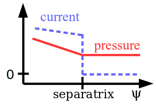
Figure 2: [Color online] Sketch that shows a discontinuous first derivative in pressure causes a discontinuous current profile when solving the Grad-Shafranov equation.

Additionally, reconstructions commonly assume that the region outside the last closed flux surface (LCFS) is current free. The pressure, temperature and density profiles are specified only up to the LCFS and are assumed to be constant outside the LCFS as illustrated in Fig. 2. For discharges with large pedestal current, as is commonly found during QH-mode, this can lead to a large discontinuity in the current density at the LCFS that is problematic for MHD modeling. During our re-solve of the Grad-Shafranov equation, we relax the current-free assumption outside the LCFS and include temperature and density profiles with non-zero gradients which generate associated small currents in the scrape-off layer (SOL) that cause the overall current profile to be continuous. Modified-bump-function fits are used to smoothly extrapolate the pressure, electron temperature and particle density in the SOL region. Derivatives of all orders vanish for this functional fit at the edge of the SOL region and thus the resulting current profile smoothly decays to zero. For this case, the pressure drops from $922$ to $581\;Pa$, the electron temperature drops from $186$ to $30\;eV$ and the density drops from $4.6\times 10^{18}$ to $2.5\times 10^{18}\;m^{-3}$ in the SOL region. The half width of the electron pressure profile is roughly $2.5\;mm$ at the outboard mid-plane and $2\;cm$ at the divertor plate. This results in a SOL width that is slightly smaller than the measured half width of the heat-flux during the later half of the inter-ELM period of DIII-D ELMy H-mode discharges in Ref. Eich et al. (2013). These profiles fits, made with a focus on the resulting current and resistivity profiles, result in an ion-temperature profile that remains above $1\;keV$ throughout the domain. This inconsistency will be removed in future modeling. The new solution is an equilibrium that closely resembles the original reconstruction with the exception of the open-flux currents and additional quantification of these methods will be described in a future manuscript King et al. . This regenerated equilibrium is consistent with the core profiles that are measured by the high quality diagnostics on DIII-D.

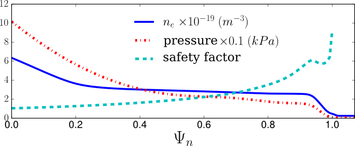
Figure 3: [Color online] Density, pressure and safety-factor profiles as a function of normalized flux. SOL profiles for density and pressure are also shown for $\psi_{n}>1$.

The density, pressure and safety-factor profiles as a function of normalized flux are shown in Fig. 3, where the SOL profiles for density and pressure are included where $\psi_{n}>1$. The current-profile that results from our re-solve of the Grad-Shafranov equation is plotted in Fig. 4. The SOL region contains small, but non-zero, currents that terminate poloidally on the divertor.

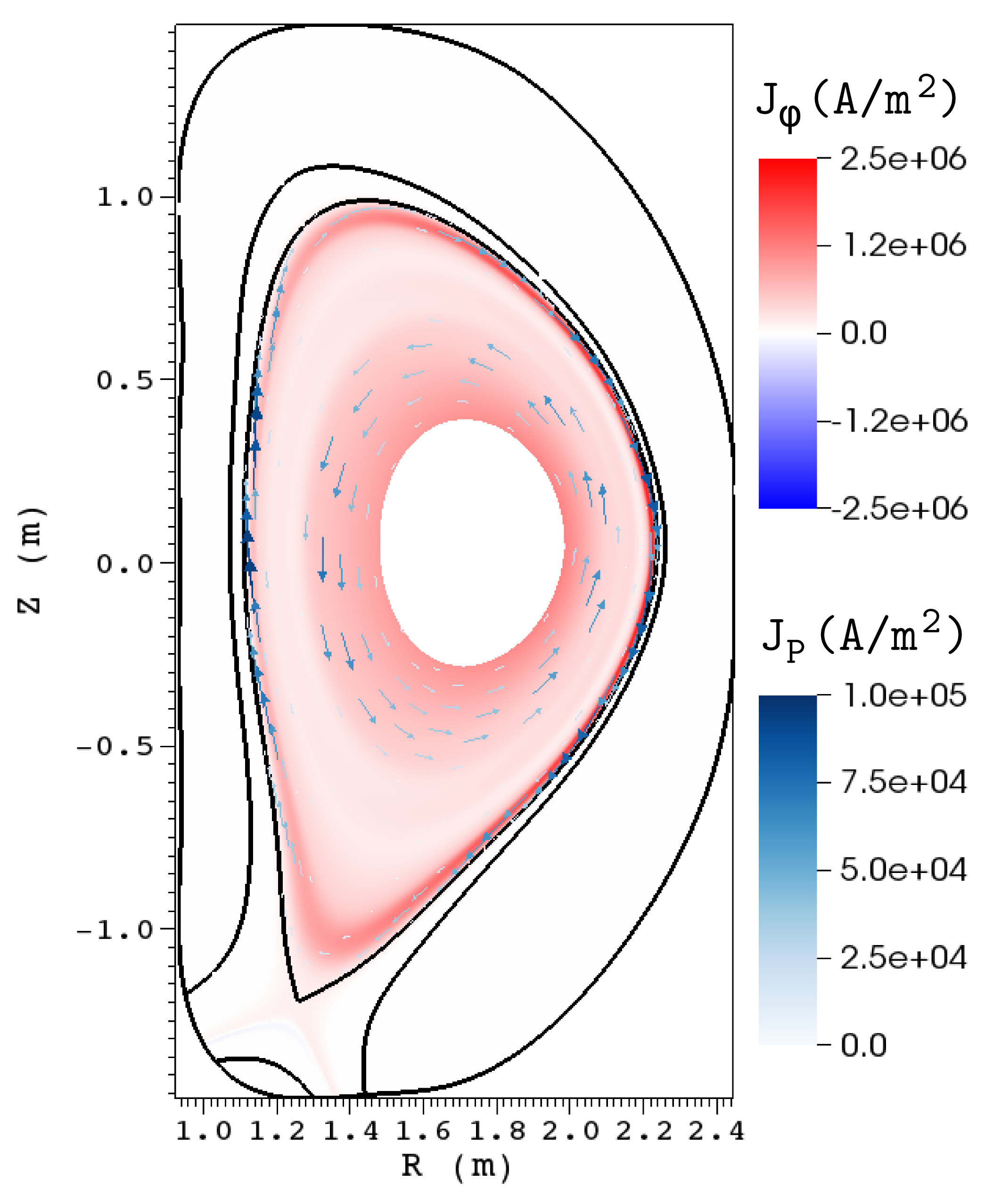
Figure 4: [Color online] Initial current density (contour colors for toroidal current and arrow vectors for poloidal current) from the reconstructed state with an extrapolated SOL region. The SOL region contains small, but non-zero currents that terminate poloidally on the divertor.

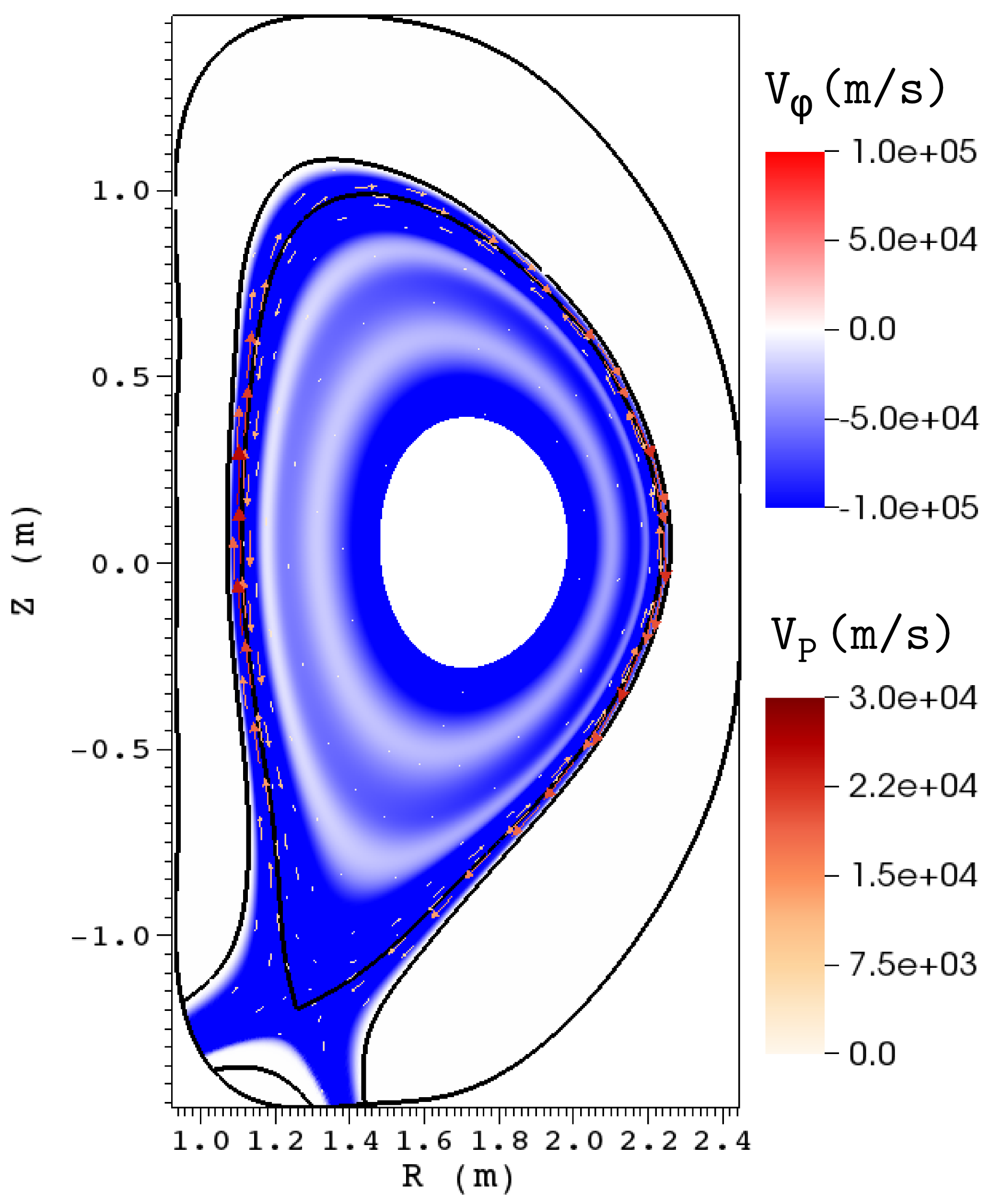
Figure 5: [Color online] The reconstructed toroidal (contour colors) and poloidal (arrow vector) flow with extrapolated flows in the SOL region. The poloidal flow flips sign just inside the LCFS with flows closer to the core proceeding counter-clockwise and flows near and outside the LCFS proceeding clockwise.

Importantly, our initial conditions include the full reconstructed toroidal and poloidal flows as shown in Fig. 5. Experimentally, these flows are critical to the observation of QH-mode where, in particular, large $\mathbf{E}\times\mathbf{B}$ flow shear is highly correlated with quiescent operation Garofalo et al. (2011). Like the thermodynamic profiles, the flow profiles are specified up to and are non-zero at the LCFS. Thus we extrapolate these profiles to zero within the SOL.

Typically only MHD-force balance (a Grad-Shafranov solution) is strictly enforced for the steady state. In practice, perturbations about a time-independent equilibrium are evolved, and that the time-independent equilibrium need not be a time-independent solution of the source-free resistive MHD equations Sovinec et al. (2004); Charlton et al. (1986). This effectively assumes the presence of implicit (in the sense that they are calculable but not calculated) sources, fluxes and sinks. With these assumptions, if the code is run on a MHD-stable case with $n_{\phi}>0$ perturbations, the modification to the $n_{\phi}=0$ fields is insignificant. Alternatively, when the case is MHD-unstable, the initial $n_{\phi}=0$ fields are self-consistently modified by the presence of the unstable modes.

The NIMROD code has the capability to compute the extended-MHD evolution of the reconstructed fields. However, it is well-known that physical mechanisms outside the scope of our modeling equations mediate tokamak transport such as neoclassical bootstrap current, toroidal viscosity, and poloidal flow damping, neutral beam and RF drives, kinetic turbulence, and coupling to the scrape-off layer (SOL), neutrals, impurities and the material boundary. Including these effects requires explicit calculation of the sources, fluxes and sinks. These transport-type calculations are possible and are becoming practical (e.g. Jenkins and Kruger (2012); Jenkins and Held (2015); Held et al. (2015)), but this sort of integrated modeling remains in the future. Thus in this work we assume that the initial reconstructed fields are steady state and our goal is to model the evolution of the 3D perturbations around this state.

III Nonlinear evolution

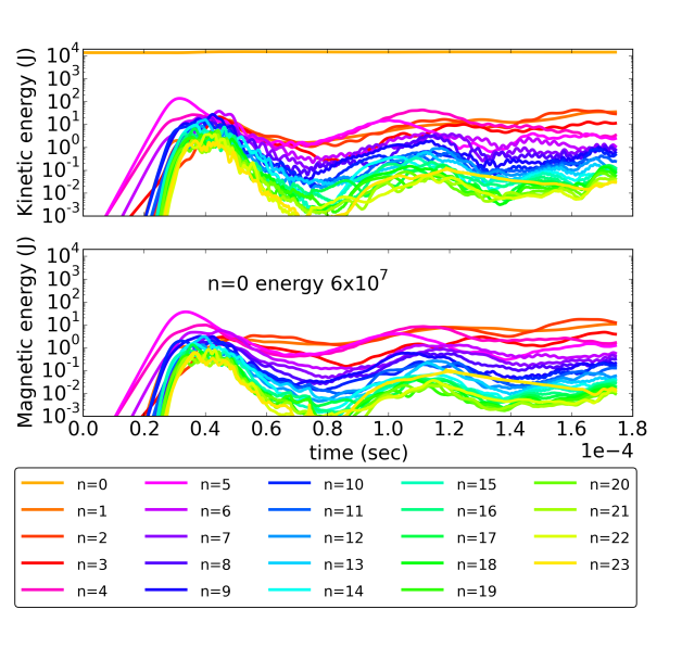
Figure 6: [Color online] Simulated kinetic and magnetic energy decomposed by toroidal mode number ($n_{\phi}$).

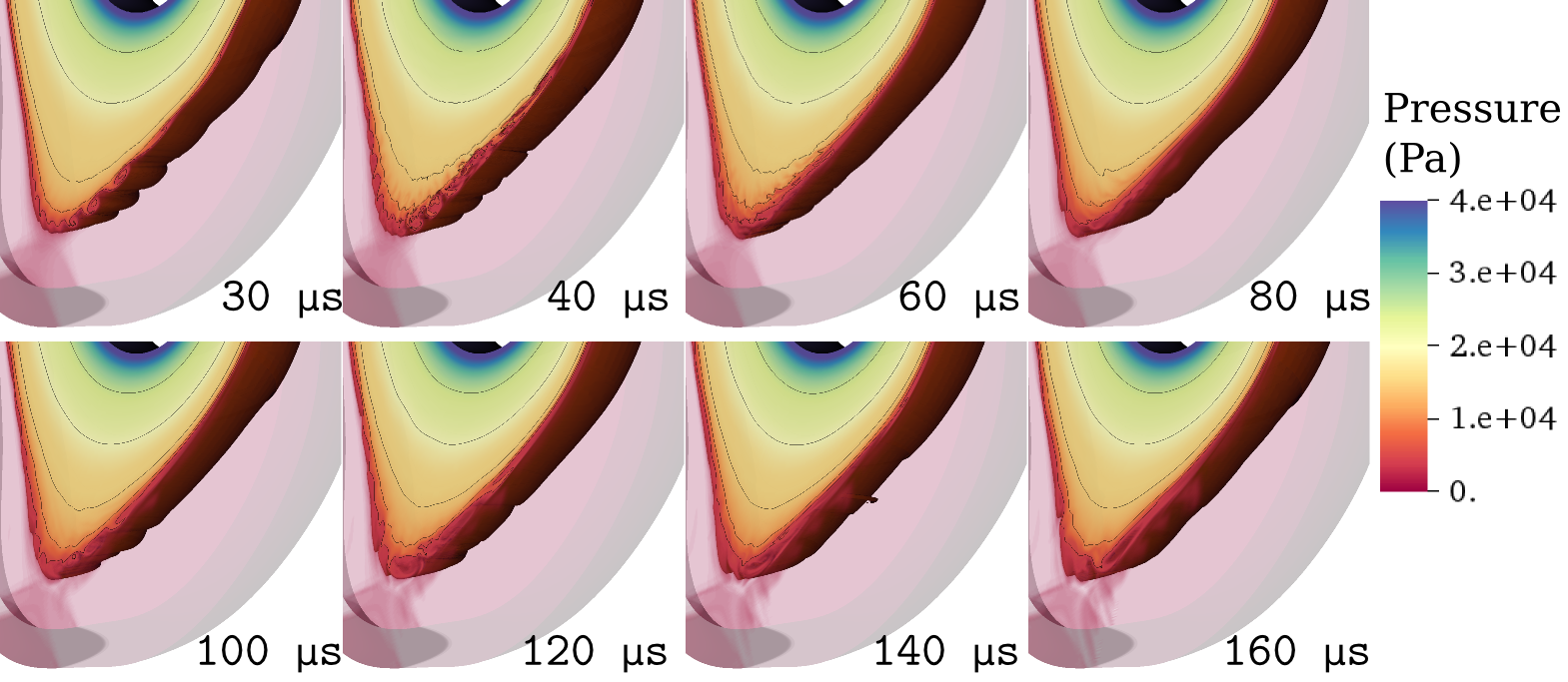
Figure 7: [Color online] A slice of the 3D domain that shows the evolution of the pressure contours at eight different times. During the initial stages (t=$30$ and $40\;\mu s$), eddies of hot, high density plasma are ejected from the pedestal and are advected poloidally in the counter-clockwise direction. Later in time these eddies are sheared apart and the dynamics become a more turbulent-like state with smoke-like off gassing which precesses poloidally counter-clockwise.

The nonlinear simulation uses a single-fluid, single-temperature (assuming fast equilibration in the perturbations) MHD model with a temperature-dependent resistivity profile where the Lundquist number, $S$, in the core is $1.1\times 10^{6}$. Here $S=\tau_{R}/\tau_{A}$, where $\tau_{A}$ is the Alfvén time ($\tau_{A}=R_{o}/v_{A}$), $v_{A}$ is the Alfvén velocity ($B/\sqrt{m_{i}n_{i}\mu_{0}}$), $\tau_{R}$ is the resistive diffusion time ($\tau_{R}=R_{o}^{2}\mu_{0}/\eta$), $R_{o}=1.748m$ is the radius of the magnetic axis, $\eta$ is the electrical resistivity, $\mu_{0}$ is the permeability of free space, $m_{i}$ is the ion mass, and $n_{i}$ is the ion density. This choice of resistivity is enhanced by a factor of 100 relative to the Spitzer value for computational practicality. The model includes large parallel and small perpendicular diffusivities in the momentum and energy equations. The parallel-momentum-stress contribution is

$$\mathbf{\Pi}_{\parallel i}=m_{i}n_{i}\nu_{\parallel i}\left(\hat{\mathbf{b}}\hat{\mathbf{b}}-\frac{1}{3}\mathbf{I}\right)\left(3\hat{\mathbf{b}}\cdot\nabla\mathbf{v}_{i}\cdot\hat{\mathbf{b}}-\nabla\cdot\mathbf{v}_{i}\right)\;,$$ (1)

where $\mathbf{v}_{i}$ is the ion velocity, $\hat{\mathbf{b}}=\mathbf{B}/|B|$, $\mathbf{I}$ is the identity tensor, and $\nu_{\parallel i}=10^{5}\;m^{2}/s$. The parallel-heat-flux contribution is

$$\mathbf{q}_{\parallel}=-n_{i}\chi_{\parallel}\hat{\mathbf{b}}\hat{\mathbf{b}}\cdot\nabla T\;,$$ (2)

where $T$ is the temperature and $\chi_{\parallel}=10^{8}\;m^{2}/s$. The small perpendicular diffusivites are modeled as isotropic particle, momentum and thermal diffusivities with a magnitude of $1\;m^{2}/s$.

The 3D nonlinear simulation is performed with a $60\times 128$ high-order (biquartic) finite element mesh packed around the pedestal region to resolve the poloidal plane and $24$ Fourier modes in the toroidal direction. The simulation is initialized from a linear computation of modes with a restricted toroidal mode number range ($n_{\phi}=1-8$). The mode energies at $t=0s$ are small, the largest energy is contained within the $n_{\phi}=4$ mode which has a spectral kinetic energy content of $4.2\times 10^{-5}\;J$ and a spectral magnetic energy content of $4.4\times 10^{-6}\;J$.

The boundary conditions, on both the inner annulus and outer wall, are no-slip for the velocity, Dirichlet for the density and temperature and a perfectly conducting wall boundary condition for the magnetic field. Linear computations show that the mode growth rates are unaffected by presence of the inner boundary, however there is an important effect in nonlinear computations. The Dirichlet condition on density and temperature provides an unrestricted particle and energy source in the core to maintain the profiles at the inner boundary in the presence of fluctuation-induced transport. With respect to the outer boundary, a sheath boundary condition is not applied at the divertor and consideration of an improved divertor boundary condition is a direction for future research.

The energy evolution from a nonlinear NIMROD simulation, decomposed by toroidal mode number, of DIII-D QH-mode shot 145098 at $4250\;ms$ with broadband MHD activity is shown in Fig 6. The simulations are initially dominated by a $n_{\phi}=5$ perturbation that saturates at around $30\;\mu s$. After this time a saturated turbulent-like state develops and the $n_{\phi}=1$ and $2$ modes become dominant through an inverse cascade. Each toroidal mode in the range of $n_{\phi}=1-5$ is dominant at a different time and continued interplay between modes is observed as the simulation progresses, particularly in the kinetic energy spectrum. Figure 7 plots the lower half of a poloidal cut of the 3D pressure contours at eight different time slices. The first time slice ($30\;\mu s$) shows a coherent structure associated with the dominant $n_{\phi}=5$ mode. By $40\;\mu s$, this structure becomes sheared apart leading to a turbulent-like state at later times. Higher-time resolution plots show the perturbations are advected in the counter-clockwise direction consistent with the direction of the ion poloidal flow inside the LCFS with a smoke-like off-gassing behavior.

IV Transport induced by the MHD perturbations

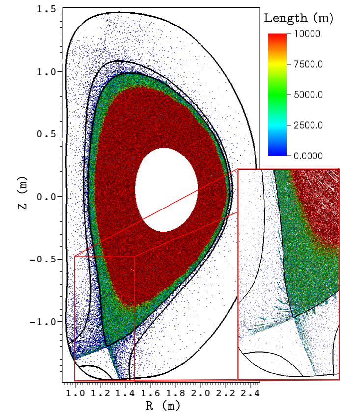
Figure 8: [Color online] Poincaré plot of magnetic fieldlines at t=$40\;\mu s$ . The pedestal region becomes stochastic where the original LCFS and SOL-region bounding contours are shown for reference. Inset shows homoclinic tangle structure near the divertor x-point.

In the presence of these electro-magnetic MHD perturbations, the pedestal region becomes stochastic as shown in Fig. 8 at t=$40\;\mu s$ by a magnetic field-line Poincaré (or puncture) plot. Field-lines in this figure are followed for $10^{4}\;m$ or until they hit the wall and then are color coded by their total length. The region from near the top of the pedestal out to the LCFS becomes stochastic. As the inset figure shows, a homoclinic tangle structure Evans et al. (2002); Roeder et al. (2003); Evans et al. (2005) develops near the divertor x-point. Given the large parallel thermal conductivity and stochastic magnetic fields, one expects significant energy transport within the pedestal region to result. However, as shown and discussed next, this is not the case and the energy transport is relatively small when compared with the particle transport.

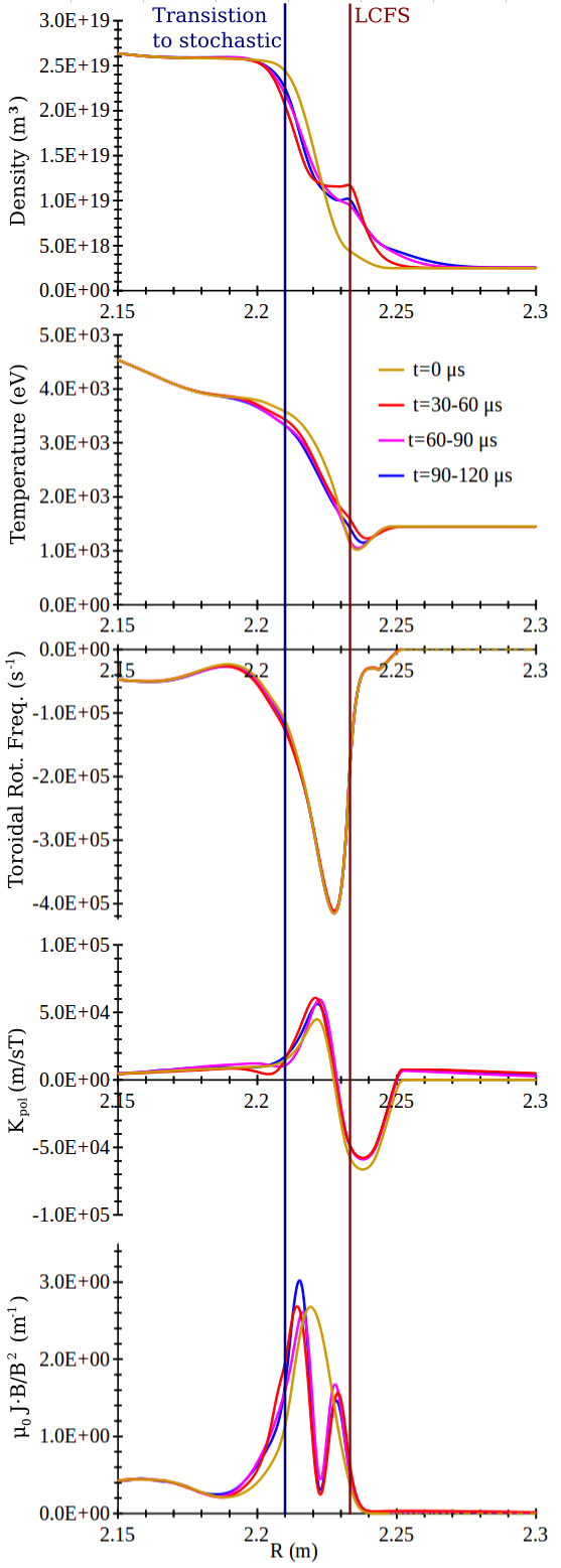
Figure 9: [Color online] Toroidal average of the density, temperature, toroidal- and poloidal-rotation, and current-density profiles on the outboard midplane for the initial condition and average values during three time windows.

Figure 9 shows the toroidal average of the density, temperature, toroidal- and poloidal-rotation, and current-density profiles on the outboard midplane for the initial conditions and average values during three time windows. The largest profile modifications occur with the density and current profiles, whereas the flow profiles are largely unchanged. Consistent with experimental observations during QH-modeGarofalo et al. (2015), the simulated state leads to large particle transport relative to the thermal transport. However, this simulation result is somewhat puzzling given the stochastic magnetic field region within the pedestal. We posit three potential explanations that require further investigation. The first possibility is that the simulation time is too short for the profiles to reach a fully relaxed state. The second theory is that the large thermal conductivity changes the phase of the temperature perturbation relative to the density perturbation in such a way that the flux-surface-averaged advective transport (where the particle flux is $(d/dV)\int_{V}\tilde{n}\tilde{\mathbf{v}}\cdot\nabla\psi/|\nabla\psi|dV$ and the thermal flux is roughly $(d/dV)\int_{V}\tilde{T}\tilde{\mathbf{v}}\cdot\nabla\psi/|\nabla\psi|dV$; here $V$ is the volume enclosed by a flux surface) is large for the plasma density but small for the plasma energy. A third hypothesis is that the stochastic transport is small because the temperature in the open-field line region is large ($\simeq 1\;keV$) and thus the effective temperature gradient along the field-lines is small. For this computation, the pressure profile (and thus implicitly the temperature profile) in the SOL was chosen to minimize the SOL currents. Future computation will include temperatures in the open-flux region that are at least an order of magnitude smaller. The experimentally relevant value is somewhat difficult to determine as the ion temperature profile is not well constrained in the open-field-line region. Given the relatively low density outside the LCFS, the CER measurements can be corrupted by effects from confined particles with large banana orbits from the higher-density pedestal region.

V Discussion and Conclusions

With regard to the saturation mechanism of the unstable modes, there are two avenues to saturation from a spectral energy perspective: (1) The unstable perturbations can directly modify the mean fields and eliminate the source of free energy by relaxing the profile gradients; or (2) the perturbations can couple to stable modes that dissipate the energy (again through modification of the mean fields or through energy flow to the boundary of the domain). Figure 9 shows that the perturbations in this case make non-trivial modifications to the $n_{\phi}=0$ fields that relax the pressure gradient and current profile leading to saturation.

One complication to this picture arises when considering the steady-state nature of the initial state from the reconstructed fields. As mentioned in Sec. II, these fields are assumed to be time independent given the presence of sources, sinks and fluxes that are outside the scope of our modeling. For a discharge state with broadband MHD activity, the contribution of the flux from the MHD perturbations is included in the steady-state assumption. In this sense, our modeling of the transport from the MHD perturbations constitutes a ‘double counting’ of this flux. For studies that compare the level of this flux to experiment there are two approaches to resolve this inconsistency: (1) The initial profiles could differ from the experiment and be more unstable such that the MHD perturbations relax the profiles to a state that resembles the reconstructed profiles; or (2) the $n_{\phi}=0$ modifications from the MHD perturbations could be cancelled (or ignored) such that the final profiles match the reconstructed values. This first approach suffers from the difficulty of finding the more unstable state, a priori, that relaxes to the reconstructed state. The second approach is the traditional way turbulent flux calculations are performed and is of interest for future studies. As this approach eliminates mode saturation through modification of the mean fields, the stability of the mode spectrum becomes critical. In particular, it is likely that simulations must be performed with an extended-MHD model that includes two-fluid, first-order finite-Larmour-radius effects that stabilize the intermediate-$n_{\phi}$ modes.

Our simulations produce an MHD turbulent-like state, which is a good candidate to at least partially explain the broadband-MHD phenomena. However, additional comparisons to experimental data are required to confidently claim these simulations truly model the discharge dynamics. Prior attempts to compare with magnetic probe data proved unsuccessful as the probe measurement temporal resolution (200 kHz) is approximately two orders of magnitude smaller than our nonlinear simulation time period. Higher time-resolution measurements that make local measurements of the perturbations (e.g. beam-emission spectroscopy and Doppler reflectometry) are a more promising avenue to pursue validation and will be the subject of future studies.