Optical Random Riemann Waves in Integrable Turbulence

Abstract

We examine integrable turbulence (IT) in the framework of the defocusing cubic one-dimensional nonlinear Schrödinger equation. This is done theoretically and experimentally, by realizing an optical fiber experiment in which the defocusing Kerr nonlinearity strongly dominates linear dispersive effects. Using a dispersive-hydrodynamic approach, we show that the development of IT can be divided into two distinct stages, the initial, pre-breaking stage being described by a system of interacting random Riemann waves. We explain the low-tailed statistics of the wave intensity in IT and show that the Riemann invariants of the asymptotic nonlinear geometric optics system represent the observable quantities that provide new insight into statistical features of the initial stage of the IT development by exhibiting stationary probability density functions.

Propagation of nonlinear random waves has recently received much attention in many areas of modern physics such as nonlinear statistical optics Picozzi et al. (2014); Laurie et al. (2012); Turitsyna et al. (2013); Pierangeli et al. (2016), hydrodynamics Herbert et al. (2010), mechanics Miquel et al. (2013), and cold-atom physics Navon et al. (2016). In all these areas a broad class of wave phenomena is modelled by integrable nonlinear partial differential equations (PDEs). Although the fundamental role of integrable PDEs has been established since the pioneering work of Fermi, Pasta and Ulam in the $1950$s Fermi et al. (1955) the significance of random input problems for such systems was realized only recently, leading to the concept of integrable turbulence (IT) Zakharov (2009); Agafontsev and Zakharov (2015); Randoux et al. (2014); Walczak et al. (2015); Suret et al. (2016); Närhi et al. (2016); Randoux et al. (2016); Zakharov et al. (2016); Agafontsev and Zakharov (2016). In this context, the one-dimensional nonlinear Schrödinger equation (1D-NLSE) plays a prominent role because it describes at leading order wave phenomena relevant to many fields of nonlinear physics.

It is now well established from experiments and numerical simulations that heavy-tailed (resp. low-tailed) deviations from gaussian statistics occur in integrable wave systems ruled by the focusing (resp. defocusing) 1D-NLSE Walczak et al. (2015); Suret et al. (2016); Randoux et al. (2014, 2016). The heavy-tailed deviations from gaussian statistics have their origin in the random formation of bright coherent structures having properties of localization in space and time similar to rogue waves Walczak et al. (2015); Suret et al. (2016); Onorato et al. (2013). On the other hand, the low-tailed deviations are due to random generation of dispersive shock waves (DSWs) and dark solitons Randoux et al. (2014, 2016). One of the key features of IT is the establishment, at long evolution time, of a state in which the statistical properties of the wave system remain stationary. Due to integrable nature of the system, the long-time statistics depends on the statistics of the input random process (cf. Agafontsev and Zakharov (2015); Randoux et al. (2014); Walczak et al. (2015); Randoux et al. (2016)). So far, there has been no satisfactory theoretical framework developed for the description of statistical features of IT due to high complexity of nonlinear wave interactions occurring over the course of its development.

In this Letter, we examine IT in optical systems described by the defocusing 1D NLSE from the perspective of dispersive hydrodynamics Biondini et al. (2016), a semi-classical theory of nonlinear dispersive waves exhibiting two distinct spatio-temporal scales: the long scale specified by initial conditions and the short scale by the internal coherence length (i.e. the typical size of the coherent structures). This scale separation enables one to split the development of IT into distinct stages characterized by qualitatively different dynamical and statistical features.

At the initial, pre-breaking stage of dispersive-hydrodynamic IT nonlinear effects dominate linear dispersion and the wave fronts of the random initial field experience gradual steepening leading to the formation of gradient catastrophes that are regularized through the generation of DSWs El and Hoefer (2016). As numerical simulations reported in ref. Randoux et al. (2016) show, the pre-breaking stage of IT is characterized by significant deviations from the gaussian statistics exhibiting the low-tailed probability density function (PDF) for the wave’s intensity, see also Fig. 1(b). In the post-breaking regime, the evolution of the statistics of the random wave field is determined by interactions among DSWs leading to further deviations from gaussianity (see ref. Randoux et al. (2016) and Fig. 1(c) showing the PDFs before the occurrence of wave breaking ($\xi=0.156$) and at long evolution distance ($\xi=1.56$), in the statistical stationary state).

In this work, we provide a quantitative explanation of the occurrence of non-gaussian statistics at the pre-breaking stage of the IT development by analysing solutions of the defocusing 1D-NLSE in the zero dispersion (nonlinear geometric optics) limit, where the dynamics can be interpreted in terms of interacting Riemann waves. Moreover, we show that Riemann invariants diagonalising the geometric optics system represent also the relevant statistical variables in IT, exhibiting stationary PDFs, in sharp contrast with evolving statistical distributions of the instantaneous power.

We consider the defocusing integrable 1D-NLSE in dimensionless form:

$$i\epsilon\frac{\partial\psi}{\partial\xi}+\frac{\epsilon^{2}}{2}\frac{\partial^{2}\psi}{\partial\tau}-|\psi|^{2}\psi=0.$$ (1)

In the optical fiber experiment realized in our work, $\psi(\xi,\tau)$ is the slowly-varying envelope of the electric field $A$ that is normalized to the square root of the mean optical power $\bar{\rho_{0}}$ of the partially coherent field propagating inside the fiber ($\psi=A/\sqrt{\bar{\rho_{0}}}$). It is usual in nonlinear fiber optics to introduce a nonlinear length $L_{NL}=1/(\gamma\bar{\rho_{0}})$ and a linear dispersion length $L_{D}=2/(\beta_{2}[\Delta\nu_{0}]^{2})$. $\gamma$ and $\beta_{2}$ are the Kerr and the second-order dispersion coefficients of the optical fiber, respectively ($\beta_{2}=+20$ps²km^-1, $\gamma=+6$W^-1km^-1, normal dispersion regime). $\Delta\nu_{0}$ represents the width of the spectrum of power fluctuations of the wave injected inside the optical fiber. With our notations, the propagation distance $z$ along the fiber is normalized as $\xi=z/\sqrt{L_{NL}L_{D}}$, the physical time $t$ is normalized as $\tau=t/T_{0}$ with $T_{0}=1/\Delta\nu_{0}$ and $\epsilon=\sqrt{L_{NL}/L_{D}}$ is the dispersion parameter which in our experiment is about $0.014$.

Considering $\epsilon$ to be a small parameter we introduce the semi-classical Madelung transformation $\psi(\xi,\tau)=\sqrt{\rho(\xi,\tau)}e^{i\frac{\phi(\xi,\tau)}{\epsilon}}$ to obtain to leading order in $\epsilon$ the nonlinear geometric optics equations for the the instantaneous power $\rho(\xi,\tau)$ and the instantaneous frequency $u(\tau,\xi)=\phi_{\tau}$ of the optical wave Forest et al. (2009); Wabnitz et al. (2013); Fatome et al. (2014); Kodama and Wabnitz (1995); Moro and Trillo (2014)

$$\rho_{\xi}+(\rho u)_{\tau}=0,\qquad u_{\xi}+uu_{\tau}+\rho_{\tau}=0\,.$$ (2)

Eqs. (2) are identical to the shallow-water equations for an incompressible fluid with $\rho>0$ and $u$ interpreted as the fluid height and the depth-averaged horizontal fluid velocity respectively and with the roles of space $\xi$ and time $\tau$ interchanged. System (2) was rigorously proved in Jin et al. (1999) to describe the pre-breaking NLS dynamics in the semi-classical ($\epsilon\to 0$) limit.

Upon introducing Riemann invariants $r_{1,2}(\xi,\tau)=u\pm 2\sqrt{\rho}$ as new variables, the system (2) becomes El and Hoefer (2016)

$$\frac{\partial r_{1,2}}{\partial\xi}+V_{1,2}\frac{\partial r_{1,2}}{\partial\tau}=0,\quad V_{1,2}=\frac{3}{4}r_{1,2}+\frac{1}{4}r_{2,1}.$$ (3)

For non-constant $r_{1,2}$ system (3) describes the propagation of two interacting Riemann waves (RWs) Whitham (2011).

Fig. 1 shows a typical result of the numerical integration of Eq. 1 by taking a random field $\psi(\xi=0,\tau)$ having gaussian statistics as initial condition. This random initial field is composed of a sum of independent Fourier modes with random phases, see Supplemental Material and ref. Randoux et al. (2016); Nazarenko (2011). Fig. 1 reveals the contrasting behaviours of dynamics and statistics of $\rho$ and $r_{1,2}$ at the pre-breaking stage of IT.

As shown in Fig. 1(a), the front edges of $\rho$ experience some steepening while the changes in $\rho$ are more pronounced at the points where the random field exhibits local maxima. At the same time, Fig. 1(b) reveals that Riemann invariants $r_{1,2}$ of the wave system behave as counterpropagating random waves, as it can be anticipated from Eq. (3).

Figure 1: Numerical simulation of Eq. (1) between $\xi=0$ and $\xi=0.156$ with $\epsilon=0.014$. Time evolution of (a) $\rho$, (b) $r_{1,2}$ and (c), (d) associated PDFs. In (c) the black dashed line represents the exponential distribution $\mathcal{P}(\rho)=e^{-\rho}$ and in (d), it represents the Rayleigh distribution ($\mathcal{P}(x)=2xe^{-x^{2}/2}$). The PDF in green line in (c) is obtained at $\xi=1.56$ where the wave system has reached a statistical stationary state.

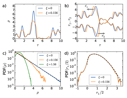
The dynamical features evidenced in Fig. 1(a),(b) determine the statistical properties characterizing IT in the pre-breaking regime. As shown in Fig. 1(c) and also previously reported in ref. Randoux et al. (2014, 2016), the PDF of $\rho$ exhibits low-tailed deviations from the exponential distribution that arise from changes in $\rho$ seen in Fig. 1(a). Contrastingly, the numerical simulations suggest that the PDFs of the Riemann invariants $r_{1,2}$ in IT remain stationary, despite the noticeable evolution of $r_{1,2}$ themselves (see Fig. 1(b) for the evolution of $r_{1,2}$ and Fig. 1(d) for the PDF of $r_{1}/2$). Moreover, as the initial velocity $u$ is close to zero, the stationary PDFs of $r_{1,2}$ are very close to the Rayleigh distribution shown in Fig. 1(d) by a dashed line.

The contrasting nature of the evolutions of the PDFs of $\rho$ and $r_{1}$ (or $r_{2}$) evidenced by the numerical simulations presented in Fig. 1 represents a striking feature that provides a new insight into the initial pre-breaking stage of the development of IT. Going beyond numerical simulations, we have used an analytical approach to investigate dynamical and statistical features typifying random Riemann waves.

First, we show that the dynamical evolution presented in Fig. 1(a) can be analyzed from the shallow water equations (2) with random initial conditions $\rho(\tau,0)=\rho_{0}(\tau)$, $u(\tau,0)=u_{0}(\tau)$, whose statistics is defined by the input Gaussian process $\psi(\tau,0)$. In our typical experimental and numerical input data, we have $u_{0}(\tau)\ll\sqrt{\rho_{0}(\tau)}$ so we shall be assuming $u_{0}(\tau)=0$ in the analytical development. Looking for the asymptotic solution of (2) in the form of “short-time” expansions for $\rho(\tau,\xi)$ and $u(\tau,\xi)$ we readily obtain for $\xi\ll 1$:

$$\rho(\tau,\xi)\simeq\rho_{0}(\tau)+\tfrac{1}{4}{[\rho_{0}^{2}(\tau)]^{\prime\prime}\xi^{2}},\ u(\tau,\xi)\simeq-\rho^{\prime}_{0}(\tau)\xi\,.$$ (4)

At the points $\tau_{m}$ of local maxima of $\rho_{0}(\tau)$ we have $[\rho_{0}^{2}(\tau_{m})]^{\prime\prime}=2\rho_{0}(\tau_{m})[\rho_{0}(\tau_{m})]^{\prime\prime}<0$ so that the first equation in (4) immediately implies the appearance of low tails in the PDF of $\rho$ due to the decrease of the maximum amplitude of the peaks of fluctuations of $\rho$ with the evolution variable $\xi$ (note that in the focusing case the expansion of $\rho$ has the same form (4) but with the minus sign for the $O(\xi^{2})$ term explaining the heavy-tailed statistics observed in Walczak et al. (2015)).

The stationary nature of the PDF of $r_{1}$ evidenced in Fig. 1(d) can be analyzed from Eq. (3) by noticing that the condition $u\ll\sqrt{\rho}$ must be satisfied at least over some propagation distance since $u_{0}(\tau)\ll\sqrt{\rho_{0}(\tau)}$. We obtain that in the regime of our interest $V_{1,2}\approx\frac{1}{2}r_{1,2}$ and Eqs. (3) can then be approximated by the system of two decoupled RWs

$$\frac{\partial r_{i}}{\partial\xi}+\frac{r_{i}}{2}\frac{\partial r_{i}}{\partial\tau}=0,\quad i=1,2.$$ (5)

Evolution of statistical parameters of random RWs has been studied in the context of Burgers turbulence Gurbatov et al. (1991). One of the straightforward results of the developed theory is that the PDF $\mathcal{P}(r;\xi)$ of a random RW field $r(\tau,\xi)$ is invariant with respect to the $\xi$-evolution, i.e. $\mathcal{P}(r;\xi)=\mathcal{P}(r;0)$. The small $u$ approximation (5) of the dispersionless dynamics (2) then implies that the PDFs of the Riemann invariants $r_{1,2}$ in the full NLS equation (1) will remain stationary or almost stationary during the initial evolution of IT.

It should be emphasized that numerical simulations shown in Fig. 1 are made for the regime in which the condition $u\ll\sqrt{\rho}$ of our theoretical analysis is not fullfilled. Hence the numerical results of Fig. 1 reveal that the conservation of the PDF of Riemann invariants holds at a much longer (but still pre-breaking) evolution time, when the two RWs are coupled and their evolution is governed by Eq. (3) instead of Eq. (5). This statistical result represents an important extension of the random RWs theory Gurbatov et al. (1991) deserving further theoretical analysis.

Now we report an optical fiber experiment in which we realize the first observation of random Riemann waves in a turbulent field. Before presenting our experimental results, let us emphasize that experimental observations of RWs that have been reported so far involve the setting implying only one ‘isolated’ RW Wetzel et al. (2016); Trillo et al. (2016). In the nonlinear optics context, this corresponds to imposing a very special relation between the wave intensity and the phase gradient (chirp) Wabnitz (2013). Such specially designed optical RWs have been recently realized in optical fiber experiments reported in ref. Wetzel et al. (2016) and the wave breaking dynamics of one simple RW has been also examined in some recent hydrodynamical experiments Trillo et al. (2016).

In the context of IT, the intrinsic random nature of nonlinear waves prevents the realization of a simple setting in which the dynamics of the wave system would be given by one Riemann invariant while the other one would remain constant. This has major implications for the experiment that must be designed in order to measure not only one hydrodynamical variable but both $\rho$ and $u$ in a simultaneous way. Moreover the observation of the changes experienced by the random RWs can be made only if $\rho$ and $u$ are simultaneously measured at the input and output ends of the nonlinear medium.

Fig. 2 represents the experimental setup that we have designed to perform the measurement of Riemann invariants in the context of IT. A partially-coherent light beam at $1064$ nm is generated by a homemade source that has a narrow linewidth together with a gaussian statistics. The typical time scale characterizing power fluctuations of this light source is $T_{0}\sim 250$ ps ($\Delta\nu_{0}=4$ GHz). The optical power of the beam is amplified to $\bar{\rho_{0}}\sim 130$ mW by using an Ytterbium fiber amplifier. The partially coherent light beam is linearly-polarized and it is launched inside a $1.4$ km-long polarization-maintaining (PM) single-mode optical fiber. In our experiment, the linear and nonlinear lengths are $L_{D}=6250$ km and $L_{NL}=1.3$ km ($\epsilon\sim 0.014$). The normalized propagation distance corresponding to the $1.4$ km physical distance is $\xi=0.0156$.

Figure 2: Experimental setup. Partially coherent light at $1064$ nm is injected inside a $1.4$-km-long PM fiber in a regime where nonlinear effects strongly dominate linear ones ($L_{NL}=1.3$ km, $L_{D}=6250$ km, $\epsilon=0.014$). Real-time observation of $\rho(\tau)$ and of $u(\tau)$ at the input and output ends of the PM fiber is achieved by combining a time-division multiplexing technique and an heterodyne measurement (see text).

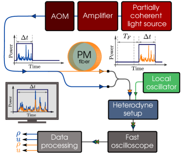
As shown in Fig. 2, the partially-coherent light wave at the input and output ends of the PM fiber is analyzed by using a heterodyne setup. The light wave is linearly mixed with an external laser source, also called local oscillator, that delivers stable single-frequency radiation at $1064$ nm. Two fast photodiodes having a bandwidth of $50$ GHz are used in the heterodyne setup to record the power fluctuations of the incoherent light wave and the beating signal between the partially-coherent light and the local oscillator. The two photodiodes are connected to a fast oscilloscope (bandwidth $65$ GHz, sampling rate $160$ GSa/s). Signals detected by the two photodiodes have been carefully synchronized with an accuracy of $\sim 3$ ps by using a mode-locked laser delivering picosecond pulses and an adjustable delay line, see Supplemental Material for details about the heterodyne measurement of $u$ and the synchronization procedure.

The experimental setup incorporates a time-division multiplexing part that enables the accurate observation of the nonlinear changes experienced by $\rho(\tau)$ and $u(\tau)$ between the input and the output ends of the PM fiber. An acousto-optic modulator (AOM) is used to periodically slice square windows with a duration $\Delta T=5.7\mu$s $\gg T_{0}\sim 250$ps in the light wave that is injected inside the PM fiber. A $50/50$ fiber coupler is used to combine light beams at the input and at the output ends of the PM fiber. Hence the heterodyne setup periodically analyzes input light fluctuations and subsequently, output light fluctuations that are delayed by a time $T_{F}\sim 7$ $\mu$s associated with propagation inside the PM fiber. Computing the autocorrelation function of the power fluctuations $P(t)$, we have been able to measure $T_{F}$ with an accuracy of $\pm 3$ ps. Data have been processed in such a way that light fluctuations at the output of the fiber are shifted backward in time by $T_{F}$, which permits the direct observation of the nonlinear changes experienced by $\rho(\tau)$ and $u(\tau)$ inside the PM fiber.

Figure 3: Experiments. Time evolution of $\rho$, $u$, and of the Riemann invariants $r_{1,2}=u\pm 2\sqrt{\rho}$ at the input end ($\xi=0$) and at the output end ($\xi=0.0156$) of the fiber ($T_{0}=250$ ps). The black dashed lines represent Riemann invariants calculated from numerical integration of Eqs. (5) while starting from the experiment initial conditions (blue lines).

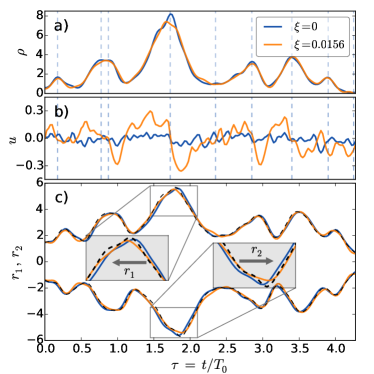
As shown in Fig. 3(a), the experiment reveals dynamical features for $\rho(\tau)$ that are similar to those evidenced by numerical simulations of Fig. 1(a). As shown in Fig. 3(b), the experiment also reveals that the instantaneous frequency $u(\tau)$ does not change in regions where $\rho(\tau)$ reaches extrema, see vertical dashed lines in Fig. 3(a)(b) indicating that the positions of maxima of $\rho$ coincide with positions where $u$ stays close to zero. This experimental result is in full agreement with the expression obtained for $u$ in Eq. 4.

Fig. 3(c) shows the two Riemann invariants $r_{1,2}=u\pm 2\sqrt{\rho}$ that are computed from the data plotted in Fig. 3(a)(b). The evolution plotted in Fig. 3(c) agrees quite well with the one given by Eq. (5). The Riemann invariants evolve as two waves that propagate in opposite directions. Even though the evolution captured by the experiment between $\xi=0$ and $\xi=0.0156$ is much less pronounced than the one evidenced by numerical simulations of Fig. 1, it should be emphasized that it is nevertheless significant and in reasonably good agrement with the evolution predicted by Eq. (5). Indeed, the dashed black lines in Fig. 3(c) represent the result of the numerical integration of Eq. (5) between $\xi=0$ and $\xi=0.0156$ while starting from initial conditions recorded in the experiment. The obtained agreement between experiments and numerical simulations is acceptable without being perfect because of limited signal to noise ratio in the measurement of $\rho$ and $u$.

Figure 4: Experimental PDFs of (a) $\rho$, (b) $r_{1}/2$. Blue (resp. yellow) lines represent PDFs at the input (resp. output) end of the fiber. In (a) the black dashed line represents the exponential distribution and in (b), it represents the Rayleigh distribution.

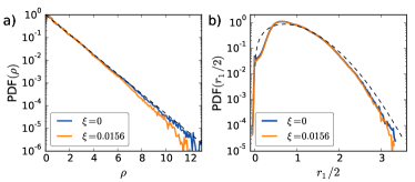
Statistical features typifying dispersive-hydrodynamic IT have been investigated from long time series lasting $500\mu$s and including $80.10^{6}$ points. As shown in Fig. 4(a), the evolution depicted by the PDF of $\rho$ is qualitatively similar to the one evidenced in Fig. 1(c) and also in ref. Randoux et al. (2014). On the other hand, as implied by the approximate decoupled RW system (5) the PDF of the Riemann invariant $r_{1}/2$ practically does not change with $\xi$: it is found to nearly retain the shape of the (initial) Rayleigh distribution (note that initially $R_{1,2}\approx\pm 2\sqrt{\rho}$), see Fig. 4(c). Note that $\sim 2\%$ of the measured points were excluded from the statistical analysis giving the PDFs of $u$ and $r_{1}/2$. For those points, the value of $\rho$ is indeed too small for the proper determination of $u$.

In conclusion, we have examined the development of IT from the perspective of dispersive hydrodynamics. Within this framework the initial stage of the IT development is described by a system of two interacting random Riemann waves. Our analysis provides an elementary theoretical explanation of the fundamental IT phenomenon of the appearance of low tails in the PDF of the wave’s intensity. We have also shown from an optical fiber experiment that Riemann invariants represent observable quantities that provide new insight into the description and the understanding of IT. We hope that the dispersive-hydrodynamic approach used in our work will pave the way to further theoretical and experimental studies in this field.

This work has been partially supported by the Agence Nationale de la Recherche through the LABEX CEMPI project (ANR-11-LABX-0007), the Ministry of Higher Education and Research, Hauts de France council and European Regional Development Fund (ERDF) through the the Nord-Pas de Calais Regional Research Council and the European Regional Development Fund (ERDF) through the Contrat de Projets Etat-Région (CPER Photonics for Society P4S).

References

- Picozzi et al. (2014) A. Picozzi, J. Garnier, T. Hansson, P. Suret, S. Randoux, G. Millot, and D. Christodoulides, Phys. Rep. 542, 1 (2014).
- Laurie et al. (2012) J. Laurie, U. Bortolozzo, S. Nazarenko, and S. Residori, Physics Reports 514, 121 (2012), one-Dimensional Optical Wave Turbulence: Experiment and Theory.
- Turitsyna et al. (2013) E. G. Turitsyna, S. V. Smirnov, S. Sugavanam, N. Tarasov, X. Shu, S. B. E. Podivilov, D. Churkin, G. Falkovich, and S. Turitsyn, Nat. Photon. 7, 783 (2013).
- Pierangeli et al. (2016) D. Pierangeli, F. Di Mei, G. Di Domenico, A. J. Agranat, C. Conti, and E. DelRe, Phys. Rev. Lett. 117, 183902 (2016).
- Herbert et al. (2010) E. Herbert, N. Mordant, and E. Falcon, Phys. Rev. Lett. 105, 144502 (2010).
- Miquel et al. (2013) B. Miquel, A. Alexakis, C. Josserand, and N. Mordant, Phys. Rev. Lett. 111, 054302 (2013).
- Navon et al. (2016) N. Navon, A. L. Gaunt, R. P. Smith, and Z. Hadzibabic, Nature 539, 72 (2016).
- Fermi et al. (1955) E. Fermi, J. Pasta, and S. Ulam, Los Alamos Report LA-1940 978 (1955).
- Zakharov (2009) V. E. Zakharov, Stud. Appl. Math. 122, 219 (2009).
- Agafontsev and Zakharov (2015) D. S. Agafontsev and V. E. Zakharov, Nonlinearity 28, 2791 (2015).
- Randoux et al. (2014) S. Randoux, P. Walczak, M. Onorato, and P. Suret, Phys. Rev. Lett. 113, 113902 (2014).
- Walczak et al. (2015) P. Walczak, S. Randoux, and P. Suret, Phys. Rev. Lett. 114, 143903 (2015).
- Suret et al. (2016) P. Suret, R. El Koussaifi, A. Tikan, C. Evain, S. Randoux, C. Szwaj, and S. Bielawski, Nature Communications 7 (2016).
- Närhi et al. (2016) M. Närhi, B. Wetzel, C. Billet, S. Toenger, T. Sylvestre, J.-M. Merolla, R. Morandotti, F. Dias, G. Genty, and J. M. Dudley, Nature Communications 7 (2016).
- Randoux et al. (2016) S. Randoux, P. Walczak, M. Onorato, and P. Suret, Physica D: Nonlinear Phenomena 333, 323 (2016).
- Zakharov et al. (2016) D. V. Zakharov, V. E. Zakharov, and S. A. Dyachenko, Physics Letters A 380, 3881 (2016).
- Agafontsev and Zakharov (2016) D. S. Agafontsev and V. E. Zakharov, Nonlinearity 29, 3551 (2016).
- Onorato et al. (2013) M. Onorato, S. Residori, U. Bortolozzo, A. Montina, and F. Arecchi, Phys. Rep. 528, 47 (2013).
- Biondini et al. (2016) G. Biondini, G. El, M. Hoefer, and P. Miller, Physica D: Nonlinear Phenomena 333, 1 (2016).
- El and Hoefer (2016) G. A. El and M. A. Hoefer, Physica D: Nonlinear Phenomena 333, 11 (2016).
- Forest et al. (2009) M. G. Forest, C.-J. Rosenberg, and O. C. Wright, Nonlinearity 22, 2287 (2009).
- Wabnitz et al. (2013) S. Wabnitz, C. Finot, J. Fatome, and G. Millot, Physics Letters A 377, 932 (2013).
- Fatome et al. (2014) J. Fatome, C. Finot, G. Millot, A. Armaroli, and S. Trillo, Phys. Rev. X 4, 021022 (2014).
- Kodama and Wabnitz (1995) Y. Kodama and S. Wabnitz, Opt. Lett. 20, 2291 (1995).
- Moro and Trillo (2014) A. Moro and S. Trillo, Phys. Rev. E 89, 023202 (2014).
- Jin et al. (1999) S. Jin, C. D. Levermore, and D. W. McLaughlin, Communications on Pure and Applied Mathematics 52, 613 (1999).
- Whitham (2011) G. B. Whitham, Linear and nonlinear waves, vol. 42 (John Wiley & Sons, 2011).
- Nazarenko (2011) S. Nazarenko, Wave Turbulence. 10.1007/978-3-642-15942-8, Lecture Notes in Physics (Springer Berlin Heidelberg, Berlin, Heidelberg, 2011).
- Gurbatov et al. (1991) S. N. Gurbatov, A. Malakhov, and A. I. Saichev, Nonlinear random waves and turbulence in nondispersive media: waves, rays, particles (Manchester University Press, 1991).
- Wetzel et al. (2016) B. Wetzel, D. Bongiovanni, M. Kues, Y. Hu, Z. Chen, S. Trillo, J. M. Dudley, S. Wabnitz, and R. Morandotti, Phys. Rev. Lett. 117, 073902 (2016).
- Trillo et al. (2016) S. Trillo, G. Deng, G. Biondini, M. Klein, G. F. Clauss, A. Chabchoub, and M. Onorato, Phys. Rev. Lett. 117, 144102 (2016).
- Wabnitz (2013) S. Wabnitz, Journal of Optics 15, 064002 (2013).