The effect of immigrant communities coming from higher incidence tuberculosis regions to a host country

Abstract

We introduce a new tuberculosis (TB) mathematical model, with $25$ state-space variables where $15$ are evolution disease states (EDSs), which generalises previous models and takes into account the (seasonal) flux of populations between a high incidence TB country (A) and a host country (B) with low TB incidence, where (B) is divided into a community (G) with high percentage of people from (A) plus the rest of the population (C). Contrary to some beliefs, related to the fact that agglomerations of individuals increase proportionally to the disease spread, analysis of the model shows that the existence of semi-closed communities are beneficial for the TB control from a global viewpoint. The model and techniques proposed are applied to a case-study with concrete parameters, which model the situation of Angola (A) and Portugal (B), in order to show its relevance and meaningfulness. Simulations show that variations of the transmission coefficient on the origin country has a big influence on the number of infected (and infectious) individuals on the community and the host country. Moreover, there is an optimal ratio for the distribution of individuals in (C) versus (G), which minimizes the reproduction number $R_{0}$. Such value does not give the minimal total number of infected individuals in all (B), since such is attained when the community (G) is completely isolated (theoretical scenario). Sensitivity analysis and curve fitting on $R_{0}$ and on EDSs are pursuit in order to understand the TB effects in the global statistics, by measuring the variability of the relevant parameters. We also show that the TB transmission rate $\beta$ does not act linearly on $R_{0}$, as is common in compartment models where system feedback or group interactions do not occur. Further, we find the most important parameters for the increase of each EDS.

Keywords:

tuberculosis; mathematical model; flux of populations; sensitivity analysis; curve fitting; reproduction number.

Mathematics Subject Classification 2010:

92D30.

1 Introduction

Tuberculosis (TB) is an infectious disease caused by the Mycobacterium tuberculosis (Mtb). Following the World Health Organization (WHO), the (Mtb) is the second cause of death worldwide from a single infectious agent, after the human immunodeficiency virus [29]. TB is present in all regions of the world. Most of the estimated number of cases in 2013 occurred in Asia ($56\%$) and the African region ($29\%$); smaller proportions of cases occurred in the Eastern Mediterranean region ($8\%$), the European region (4%) and the region of the Americas ($3\%$) [30].

In TB spread, migration plays an important role, e.g., following the International Organization for Migration (IOM), TB is a social disease and migration, as a social determinant of health, increases TB-related morbidity and mortality among migrants and surrounding communities [10]. Migrants of specific legal and social status, such as workers, undocumented migrants, trafficked and detained persons, face particular TB vulnerabilities. Among migrant workers with a legal status, their access to TB diagnosis and care is subject to their ability to access health care services and health insurance coverage, provided either by the state or the employer. Illegal migrants face particular challenges such as fear of deportation that delay or limit their access to diagnostic and treatment services. Deportation while on treatment or poor compliance with treatment may lead to drug resistant infection and increased chances of spreading TB in countries of origin, transit and destination [10].

Mathematical models are an important tool in analyzing the spread and control of infectious diseases [7, 8]. There are many mathematical dynamic models for TB, see, e.g., [1, 3, 4, 6, 27] and references cited therein. There are also models dedicated to study TB transmission dynamics in immigrants and local population. Usually, these models divide the total population into two subgroups: immigrants and local subpopulation. Each subgroup is divided into several epidemiological compartments: susceptible, latent, infectious, recovered, or other, depending on the type of the model, see, e.g., [2, 11, 32, 33]. In general, compartment models written with ordinary differential equations tend to be nice approximations of the true scenario that have rather simple formulation, e.g., with five state-space variables and a (non)autonomous quadratic vector field, because of numerical and analytic limitations and the tradeoff between complexity and the relevant information that they can present. In particular, heterogeneous situations may be studied using such models. However, no interaction between individuals in the different groups are considered in such models. We are interested in understanding how the flux and distribution of individuals affects TB on a host country. As a case-study, we have considered the situation of Angola and Portugal, although the techniques may be applied to any similar situation.

Angola is the seventh-largest country in Southern Africa with a total population of approximately $24.3$ million [9]. WHO predicts that by 2017 the TB cases rate may rise significantly in Angola. A natural question is to try to understand how this may affect the rest of the world. According to Celestino Teixeira, the Coordinator of the Fight Against Tuberculosis Programme, in 2013 Angola reported a total of $60,807$ cases of TB in all forms, observing an increase of $11\%$ over the previous year [39]. Portugal is a country in Southwest Europe with a total population of approximately $10.5$ million [9]. In 2014, for the first time, the incidence of TB in Portugal was estimated to be lower than $20$ new cases per $100,000$ inhabitants, placing Portugal among the countries with low TB incidence. However, there are still some regions (Lisbon and Porto) with much higher TB incidences [17]. Portugal is a relevant geographically area of study for TB because its infection behaviour is not similar to the rest of Europe, in the sense that has higher incidence of tuberculosis. Aside from the independence period, Angola is characterized by a reduced emigration and is becoming gradually an attractive region, receiving migrants from different regions, including Portugal [19]. Following the Portuguese Emigration Observatory, in 2014 there were 126,356 Portuguese emigrants living in Angola [40]. According to the Organisation for Economic Co-operation and Development (OECD) [16], for the first time in five years, 2012 saw the number of long-term entry visas grow. Visas to Angolans doubled in 2012, mainly for study. According to the Portuguese Foreigners and Borders Service, in 2012 there were 20,177 Angolans citizens living in Portugal [21]. Although Angolans living in Portugal are dispersed throughout the country, there is a very high concentration in the district of Lisbon, followed by Setúbal and Porto [15].

In this paper, we propose and study a new mathematical model for TB that generalises the one proposed in [13]. We consider three different populations: people living in a high TB incidence country (A), people living in a low TB incidence country in a semi-closed community of the high incidence country natives (G), and the other persons living in the low incidence country (C). Each of these three groups of population are subdivided into the five epidemiological categories considered in the model from [13]. Our model considers the movement of persons from the high TB incidence country to the low TB incidence country and vice-versa. We assume that the individuals that arrive and depart from the low TB incidence country are split into the ones that enter/leave the semi-closed community of the high TB incidence country natives and the ones that enter/leave other regions of the low TB incidence country. Our model is quite different from [13] and other TB models in the literature, since it has internal transfer of individuals between the subgroups, high TB incidence country, semi-closed community of high TB incidence country natives and other persons living in the low TB incidence country. We consider a case study where the low TB incidence country is represented by Portugal and the high TB incidence country is represented by Angola.

The paper is organized as follows. In Section 2, we explain how we construct our model. The basic reproduction number is algebraically and numerically computed in Section 3 for the autonomous case. This section also includes a sensitivity analysis of the basic reproduction number with respect to TB transmission rates, transfer of individuals and ratio of individuals that stay in the community versus spread in the host country. Section 4 is devoted to numerical simulations, which help us to make a qualitative sensitivity analysis for each epidemiological category of the subgroups Angola, semi-closed community of Angola natives and other persons living in Portugal, when relevant TB parameters are perturbed. We end with Section 5 of conclusions and future work.

2 Mathematical model

We construct a model with three components, based on [13], where there exists seasonal flux of population between some of the components. The model from [13] divides the total population $N$ in five epidemiological compartments: susceptible individuals ($\mathcal{S}$) that never have been in contact with (Mtb), primary infected individuals ($\mathcal{P}$) that have been infected by (Mtb) but it is not certain if the disease will progress, actively infected and infectious individuals ($\mathcal{I}$) that are not yet in treatment, latent infected individuals ($\mathcal{L}$) and under treatment individuals ($\mathcal{T}$). Susceptible individuals become primary infected at a rate $\lambda=\beta\nu\mathcal{I}$ $yrs^{-1}$, where $\beta$ is the transmission coefficient and $\nu$ is the proportion of pulmonary TB cases. A proportion $\phi$ and $(1-\phi)$ of individuals in the class $\mathcal{P}$ is transferred to the class $\mathcal{I}$ and $\mathcal{L}$, respectively, at a rate $\delta\,yrs^{-1}$. Each year, a proportion $k$ of individuals in the class $\mathcal{I}$ is detected and start TB treatment at a rate $\tau\,yrs^{-1}$, entering the class $\mathcal{T}$. It is assumed that individuals in the class $\mathcal{T}$ are neither infectious nor susceptible to reinfection. A fraction $\phi_{T}$ of individuals in class $\mathcal{T}$ is transferred to class $\mathcal{I}$ due to either treatment failure or default, while the remaining $(1-\phi_{T})$ are successfully treated and enter in the class $\mathcal{L}$. The inverse of treatment length is denoted by $\delta_{T}$. In [13], birth and death rates are assumed equal, here we assume that they can be different and we denote the recruitment rate by $\eta\,yrs^{-1}$ and the death rate by $\mu\,yrs^{-1}$. The reinfection factor is denoted by $\sigma$ (see [13] for more details). Optimal control strategies for such model were studied in [20, 23, 24].

Let $\mathcal{S}\equiv\mathcal{S}(t)$, $\mathcal{P}\equiv\mathcal{P}(t)$, $\mathcal{I}\equiv\mathcal{I}(t)$, $\mathcal{L}\equiv\mathcal{L}(t)$, $\mathcal{T}\equiv\mathcal{T}(t)$, where $t$ represents time in years. The model described above is given by the following system of ordinary differential equations:

$$\left\{\begin{array}[]{l}\dot{\mathcal{S}}=\eta N-\left(\lambda(t)+\mu\right)\mathcal{S},\\ \dot{\mathcal{P}}=\lambda(t)\mathcal{S}+\sigma\lambda(t)\mathcal{L}-\left(\delta+\mu\right)\mathcal{P},\\ \dot{\mathcal{I}}=\phi\delta\mathcal{P}+\omega\mathcal{L}+\phi_{T}\delta_{T}\mathcal{T}-\left(\tau k+\mu\right)\mathcal{I},\\ \dot{\mathcal{L}}=(1-\phi)\delta\mathcal{P}+(1-\phi_{T})\delta_{T}\mathcal{T}-\left(\sigma\lambda(t)+\omega+\mu\right)\mathcal{L},\\ \dot{\mathcal{T}}=\tau k\mathcal{I}-\left(\delta_{T}+\mu\right)\mathcal{T}.\end{array}\right.$$ (2.1)

We have $N=\mathcal{S}+\mathcal{P}+\mathcal{I}+\mathcal{L}+\mathcal{T}$ and $\lambda(t)=\beta\nu\mathcal{I}N^{-1}$. Then

$$\dot{\lambda}=\beta\nu\left(\dot{\mathcal{I}}N^{-1}-\mathcal{I}\,N^{-2}\dot{N}\right).$$

On the other hand, $\dot{N}=(\eta-\mu)N$, so if $\eta=\mu$ then the population is constant. The system can be written in a matrix form as

$$\dot{\mathcal{X}}=\left(\beta\nu\mathcal{I}\mathcal{A}+\mathcal{B}\right)\mathcal{X}+\mathcal{C},$$ (2.2)

where $\mathcal{X}=(\mathcal{S},\mathcal{P},\mathcal{I},\mathcal{L},\mathcal{T})$,

$$\mathcal{A}=\left(\begin{array}[]{ccccc}-1&0&0&0&0\\ 1&0&0&\sigma&0\\ 0&0&0&0&0\\ 0&0&0&-\sigma&0\\ 0&0&0&0&0\end{array}\right),\quad\mathcal{B}=\left(\begin{array}[]{ccccc}-\mu&0&0&0&0\\ 0&-(\delta+\mu)&0&0&0\\ 0&\phi\delta&-(\tau k+\mu)&\omega&\phi_{T}\delta_{T}\\ 0&(1-\phi)\delta&0&-(\omega+\mu)&(1-\phi_{T})\delta_{T}\\ 0&0&\tau k&0&-(\delta_{T}+\mu)\end{array}\right),$$

and $\mathcal{C}=(\eta N,0,0,0,0)$. We can verify that the matrix $\lambda(t)\mathcal{A}+\mathcal{B}$ can be diagonalizable, so there is a semi-closed form solution for the problem (it is not closed a priori because $\lambda$ still depends on $I$ and $N$).

Suppose this system interacts with (a convex combination of) another two similar systems $\tilde{X}_{1}$ and $\tilde{X}_{2}$, in the following way: there exist functions $\gamma(t),\tilde{\gamma}(t)\in[0,1]$ and a value $\zeta\in[0,1]$ such that

$$\left\{\begin{array}[]{l}\dot{\mathcal{S}}=\eta N-\left(\lambda(t)+\gamma(t)+\mu\right)\mathcal{S}+\tilde{\gamma}(t)\left((1-\zeta)\tilde{\mathcal{S}}_{1}+\zeta\tilde{\mathcal{S}}_{2}\right),\\ \dot{\mathcal{P}}=\lambda(t)\mathcal{S}+\sigma\lambda(t)\mathcal{L}-\left(\delta+\gamma(t)+\mu\right)\mathcal{P}+\tilde{\gamma}(t)\left((1-\zeta)\tilde{\mathcal{P}}_{1}+\zeta\tilde{\mathcal{P}}_{2}\right),\\ \dot{\mathcal{I}}=\phi\delta\mathcal{P}+\omega\mathcal{L}+\phi_{T}\delta_{T}\mathcal{T}-\left(\tau k+\gamma(t)+\mu\right)\mathcal{I}+\tilde{\gamma}(t)\left((1-\zeta)\tilde{\mathcal{I}}_{1}+\zeta\tilde{\mathcal{I}}_{2}\right),\\ \dot{\mathcal{L}}=(1-\phi)\delta\mathcal{P}+(1-\phi_{T})\delta_{T}\mathcal{T}-\left(\sigma\lambda(t)+\omega+\gamma(t)+\mu\right)\mathcal{L}+\tilde{\gamma}(t)\left((1-\zeta)\tilde{\mathcal{L}}_{1}+\zeta\tilde{\mathcal{L}}_{2}\right),\\ \dot{\mathcal{T}}=\tau k\mathcal{I}-\left(\delta_{T}+\gamma(t)+\mu\right)\mathcal{T}+\tilde{\gamma}(t)\left((1-\zeta)\tilde{\mathcal{T}}_{1}+\zeta\tilde{\mathcal{T}}_{2}\right).\end{array}\right.$$ (2.3)

Adding $N=\mathcal{S}+\mathcal{P}+\mathcal{I}+\mathcal{L}+\mathcal{T}$ as a new state variable, we have

$$\left\{\begin{array}[]{l}\dot{\mathcal{S}}=\eta N-\left(\lambda+\gamma(t)+\mu\right)\mathcal{S}+\tilde{\gamma}(t)\left((1-\zeta)\tilde{\mathcal{S}}_{1}+\zeta\tilde{\mathcal{S}}_{2}\right),\\ \dot{\mathcal{P}}=\lambda\mathcal{S}+\sigma\lambda\mathcal{L}-\left(\delta+\gamma(t)+\mu\right)\mathcal{P}+\tilde{\gamma}(t)\left((1-\zeta)\tilde{\mathcal{P}}_{1}+\zeta\tilde{\mathcal{P}}_{2}\right),\\ \dot{\mathcal{I}}=\phi\delta\mathcal{P}+\omega\mathcal{L}+\phi_{T}\delta_{T}\mathcal{T}-\left(\tau k+\gamma(t)+\mu\right)\mathcal{I}+\tilde{\gamma}(t)\left((1-\zeta)\tilde{\mathcal{I}}_{1}+\zeta\tilde{\mathcal{I}}_{2}\right),\\ \dot{\mathcal{L}}=(1-\phi)\delta\mathcal{P}+(1-\phi_{T})\delta_{T}\mathcal{T}-\left(\sigma\lambda+\omega+\gamma(t)+\mu\right)\mathcal{L}+\tilde{\gamma}(t)\left((1-\zeta)\tilde{\mathcal{L}}_{1}+\zeta\tilde{\mathcal{L}}_{2}\right),\\ \dot{\mathcal{T}}=\tau k\mathcal{I}-\left(\delta_{T}+\gamma(t)+\mu\right)\mathcal{T}+\tilde{\gamma}(t)\left((1-\zeta)\tilde{\mathcal{T}}_{1}+\zeta\tilde{\mathcal{T}}_{2}\right),\\ \dot{N}=\left(\eta-\gamma(t)-\mu\right)N+\tilde{\gamma}(t)\left((1-\zeta)\tilde{N}_{1}+\zeta\tilde{N}_{2}\right).\end{array}\right.$$ (2.4)

Let $S=\mathcal{S}N^{-1}$, $P=\mathcal{P}N^{-1}$, $I=\mathcal{I}N^{-1}$, $L=\mathcal{L}N^{-1}$, $T=\mathcal{T}N^{-1}$. These variables now represent the percentage of the population in each state, i.e., $S+P+I+L+T=1$. Since

$$\dot{S} =\dot{\mathcal{S}}N^{-1}-\mathcal{S}N^{-2}\dot{N}$$

$$=\dot{\mathcal{S}}N^{-1}-SN^{-1}\left(\left(\eta-\gamma(t)-\mu\right)N+\tilde{\gamma}(t)\left((1-\zeta)\tilde{N}_{1}+\zeta\tilde{N}_{2}\right)\right)$$

$$=\dot{\mathcal{S}}N^{-1}-\left(\eta-\gamma(t)-\mu+\tilde{\gamma}(t)\left((1-\zeta)\tilde{N}_{1}+\zeta\tilde{N}_{2}\right){N}^{-1}\right)S,$$

$$=\dot{\mathcal{S}}N^{-1}-\left(M(t)-\gamma(t)-\mu\right)S,$$

with $M(t)\mathop{\stackrel{{\scriptstyle\mbox{\tiny def}}}{{=}}}\eta+\left((1-\zeta)\tilde{N}_{1}+\zeta\tilde{N}_{2}\right)\tilde{\gamma}(t)N^{-1}$, where the calculations for the other variables are similar, and adding $\lambda(t)=\beta\nu I$ as a new state variable, we have

$$\left\{\begin{array}[]{l}\dot{S}=\eta-\left(\lambda+M(t)\right)S+\tilde{\gamma}(t)\left((1-\zeta)\tilde{S}_{1}+\zeta\tilde{S}_{2}\right),\\ \dot{P}=\lambda S+\sigma\lambda L-\left(\delta+M(t)\right)P+\tilde{\gamma}(t)\left((1-\zeta)\tilde{P}_{1}+\zeta\tilde{P}_{2}\right),\\ \dot{I}=\phi\delta P+\omega L+\phi_{T}\delta_{T}T-\left(\tau k+M(t)\right)I+\tilde{\gamma}(t)\left((1-\zeta)\tilde{I}_{1}+\zeta\tilde{I}_{2}\right),\\ \dot{L}=(1-\phi)\delta P+(1-\phi_{T})\delta_{T}T-\left(\sigma\lambda+\omega+M(t)\right)L+\tilde{\gamma}(t)\left((1-\zeta)\tilde{L}_{1}+\zeta\tilde{L}_{2}\right),\\ \dot{T}=\tau kI-\left(\delta_{T}+M(t)\right)T+\tilde{\gamma}(t)\left((1-\zeta)\tilde{T}_{1}+\zeta\tilde{T}_{2}\right),\\ \dot{\lambda}=\beta\nu\dot{I}=\beta\nu\left(\phi\delta P+\omega L+\phi_{T}\delta_{T}T-\left(\tau k+M(t)\right)I+\tilde{\gamma}(t)\left((1-\zeta)\tilde{I}_{1}+\zeta\tilde{I}_{2}\right)\right),\\ \dot{N}=\left(M(t)-\gamma(t)-\mu\right)N.\end{array}\right.$$ (2.5)

Using the above model, we consider different population groups: people living in a high incidence TB country (A) and people living in a low incidence TB country (B), where (B) is subdivided in a community (G) with high percentage of people from (A), and (C) is the rest of the population of (B). We consider that the values of $\beta$, $\nu$, $\phi_{T}$ of the group (G) are different from the values of the group (C). The flux of population follow the distribution functions $\gamma_{A}$, from (A) to (B), and $\gamma_{B}$, from (B) to (A). We assume that the persons that arrive and departure from (B) are split in the following proportions: $\zeta$ goes to (G) and $(1-\zeta)$ goes to (C), with $\zeta\in[0,1]$ a fixed percentage value in this model.

This model accounts for an average moving value of persons $a^{A}$, $a^{B}$ that increases/decreases in time by the slopes $b^{A}$, $b^{B}$ and has a seasonality variation modeled by $p^{A}$, $p^{B}$, $\theta^{A}$, $\theta^{B}$. The flux of population will be modeled by the following functions:

$$\gamma_{A}(t)=a^{A}+b^{A}t+a^{A}p^{A}\cos\left(\theta^{A}t\right),\quad\mbox{ and }\quad\gamma_{B}(t)=a^{B}+b^{B}t+a^{B}p^{B}\cos\left(\theta^{B}t\right),$$ (2.6)

for constants $a^{A},a^{B},b^{A},b^{B},p^{A},p^{B},\theta^{A},\theta^{B}\in\mathbb{R}$ chosen to ensure that $0\leq\gamma_{A}(t),\gamma_{B}(t)\leq 1$ for all $t$ of the simulation.

The flux of population $\gamma_{A}(t)$, $\gamma_{B}(t)$ can be incorporated as state-space variables. In our case, the functions $\gamma^{A}$, $\gamma^{P}$ are solutions of the system of ODEs

$$\left\{\begin{array}[]{l}\dot{\gamma}_{A}=z^{A},\\ \dot{z}_{A}=-(\theta^{A})^{2}(\gamma_{A}-a^{A}-b^{A}\,t),\end{array}\right.\quad\mbox{ and }\quad\left\{\begin{array}[]{l}\dot{\gamma}_{B}=z^{B},\\ \dot{z}_{B}=-(\theta^{B})^{2}(x-a^{B}-b^{B}\,t),\end{array}\right.$$

which we add to the model (2.8)–(2.11), obtaining the complete model with $25$ state-space variables. Note that if $V_{N}=(N_{A},N_{C},N_{G})$, then

$$\dot{V}_{N}=\mathcal{A}(t)V_{N},$$ (2.7)

where

$$\mathcal{A}(t)=\left(\begin{array}[]{ccc}\eta^{A}-\mu^{A}-\gamma_{A}(t)&\gamma_{B}(t)(1-\zeta)&\gamma_{B}(t)\zeta\\ \gamma_{A}(t)(1-\zeta)&\eta^{C}-\mu^{C}-\gamma_{B}(t)&0\\ \gamma_{A}(t)\zeta&0&\eta^{C}-\mu^{C}-\gamma_{B}(t)\end{array}\right).$$

So the population evolution is only dependent on the moving distribution functions $\gamma^{A}$, $\gamma^{P}$, born rates $\eta$, and natural death rates $\mu$. Hence, we obtain the complete model composed by the four subsystems (2.8)–(2.11) composed by: (i) the variables of the high incidence TB country

$$\left\{\begin{array}[]{l}\dot{S}_{A}=\eta^{A}-\left(\lambda_{A}+M_{A}\right)S_{A}+\gamma_{B}\left((1-\zeta)S_{C}+\zeta S_{G}\right),\\ \dot{P}_{A}=\lambda_{A}S_{A}+\sigma^{A}\lambda_{A}L_{A}-\left(\delta^{A}+M_{A}\right)P_{A}+\gamma_{B}\left((1-\zeta)P_{C}+\zeta P_{G}\right),\\ \dot{I}_{A}=\phi^{A}\delta^{A}P_{A}+\omega^{A}L_{A}+\phi^{A}_{T}\delta^{A}_{T}T_{A}-\left(\tau^{A}k^{A}+M_{A}\right)I_{A}+\gamma_{B}\left((1-\zeta)I_{C}+\zeta I_{G}\right),\\ \dot{L}_{A}=(1-\phi^{A})\delta^{A}P_{A}+(1-\phi^{A}_{T})\delta^{A}_{T}T_{A}-\left(\sigma^{A}\lambda_{A}+\omega^{A}+M_{A}\right)L_{A}+\gamma_{B}\left((1-\zeta)L_{C}+\zeta L_{G}\right),\\ \dot{T}_{A}=\tau^{A}k^{A}I_{A}-\left(\delta^{A}_{T}+M_{A}\right)T_{A}+\gamma_{B}\left((1-\zeta)T_{C}+\zeta T_{G}\right),\\ \dot{\lambda}_{A}=\beta^{A}\nu^{A}\left(\phi^{A}\delta^{A}P_{A}+\omega^{A}L_{A}+\phi^{A}_{T}\delta^{A}_{T}T_{A}-\left(\tau^{A}k^{A}+M_{A}\right)I^{A}+\gamma_{B}\left((1-\zeta)I_{C}+\zeta I_{G}\right)\right),\\ \dot{N}_{A}=\left(M_{A}-\gamma_{A}-\mu^{A}\right)N_{A},\\ \end{array}\right.$$ (2.8)

(ii) the variables associated with the community in the host country

$$\left\{\begin{array}[]{l}\dot{S}_{G}=\eta^{C}-\left(\lambda_{G}+M_{G}\right)S_{G}+\gamma_{A}\zeta S_{A},\\ \dot{P}_{G}=\lambda_{G}S_{G}+\sigma^{C}\lambda_{G}L_{G}-\left(\delta^{C}+M_{G}\right)P_{G}+\gamma_{A}\zeta P_{A},\\ \dot{I}_{G}=\phi^{C}\delta^{C}P_{G}+\omega^{C}L_{G}+\phi^{G}_{T}\delta^{C}_{T}T_{G}-\left(\tau^{C}k^{C}+M_{G}\right)I_{G}+\gamma_{A}\zeta I_{A},\\ \dot{L}_{G}=(1-\phi^{C})\delta^{C}P_{G}+(1-\phi^{G}_{T})\delta^{C}_{T}T_{G}-\left(\sigma^{C}\lambda_{G}+\omega^{C}+M_{G}\right)L_{G}+\gamma_{A}\zeta L_{A},\\ \dot{T}_{G}=\tau^{C}k^{C}I_{G}-\left(\delta^{C}_{T}+M_{G}\right)T_{G}+\gamma_{A}\zeta T_{A},\\ \dot{\lambda}_{G}=\beta^{G}\nu^{G}\left(\phi^{C}\delta^{C}P_{G}+\omega^{C}L_{G}+\phi^{G}_{T}\delta^{C}_{T}T_{G}-\left(\tau^{C}k^{C}+M_{G}\right)I^{G}+\gamma_{A}\zeta I_{A}\right),\\ \dot{N}_{G}=\left(M_{G}-\gamma_{B}-\mu^{C}\right)N_{G},\\ \end{array}\right.$$ (2.9)

(iii) the variables related with the population of the host country excluding the community

$$\left\{\begin{array}[]{l}\dot{S}_{C}=\eta^{C}-\left(\lambda_{C}+M_{C}\right)S_{C}+\gamma_{A}(1-\zeta)S_{A},\\ \dot{P}_{C}=\lambda_{C}S_{C}+\sigma^{C}\lambda_{C}L_{C}-\left(\delta^{C}+M_{C}\right)P_{C}+\gamma_{A}(1-\zeta)P_{A},\\ \dot{I}_{C}=\phi^{C}\delta^{C}P_{C}+\omega^{C}L_{C}+\phi^{C}_{T}\delta^{C}_{T}T_{C}-\left(\tau^{C}k^{C}+M_{C}\right)I_{C}+\gamma_{A}(1-\zeta)I_{A},\\ \dot{L}_{C}=(1-\phi^{C})\delta^{C}P_{C}+(1-\phi^{C}_{T})\delta^{C}_{T}T_{C}-\left(\sigma^{C}\lambda_{C}+\omega^{C}+M_{C}\right)L_{C}+\gamma_{A}(1-\zeta)L_{A},\\ \dot{T}_{C}=\tau^{C}k^{C}I_{C}-\left(\delta^{C}_{T}+M_{C}\right)T_{C}+\gamma_{A}(1-\zeta)T_{A},\\ \dot{\lambda}_{C}=\beta^{C}\nu^{C}\left(\phi^{C}\delta^{C}P_{C}+\omega^{C}L_{C}+\phi^{C}_{T}\delta^{C}_{T}T_{C}-\left(\tau^{C}k^{C}+M_{C}\right)I^{C}+\gamma_{A}(1-\zeta)I_{A}\right),\\ \dot{N}_{C}=\left(M_{C}-\gamma_{B}-\mu^{C}\right)N_{C},\\ \end{array}\right.$$ (2.10)

(iv) and the variables measuring the flux of population

$$\left\{\begin{array}[]{l}\dot{\gamma}_{A}=z^{A},\\ \dot{z}_{A}=-(\theta^{A})^{2}(\gamma_{A}-a^{A}-b^{A}\,t),\\ \dot{\gamma}_{B}=z^{B},\\ \dot{z}_{B}=-(\theta^{B})^{2}(\gamma_{B}-a^{B}-b^{B}\,t),\end{array}\right.$$ (2.11)

where for presentation convenience we define

$$M_{A} =\eta^{A}+\left((1-\zeta)N_{C}+\zeta N_{G}\right)\gamma_{B}N_{A}^{-1},$$

$$M_{C} =\eta^{C}+(1-\zeta)\gamma_{A}N_{A}N_{C}^{-1},$$

$$M_{G} =\eta^{C}+\zeta\gamma_{A}N_{A}N_{G}^{-1}.$$

Note that

$$\dot{N}_{A}+\dot{N}_{C}+\dot{N}_{G} =(\eta^{A}-\mu^{A})N_{A}+(\eta^{C}-\mu^{C})(N_{C}+N_{G}).$$

Again, if $\eta^{A}=\mu^{A}$ and $\eta^{C}=\mu^{C}$, then the total population is constant. Moreover, if $b^{A}=b^{B}=p^{A}=p^{B}=0$, then system (2.8)–(2.11) is autonomous. For notation clarity, all parameters (i.e., constant values) have upper indices whereas state variables have lower indices.

Figure 1: Model for TB transmission.

Figure 2: Flow chart between high TB incidence country (A), natives from high TB incidence country living in Communities (G) in a low TB incidence country, remainder of population living in a low TB incidence country (C).

3 Reproduction number and its sensitivity analysis for the autonomous case

The transmissibility of an infection can be asymptotically quantified by its reproduction number $R_{0}$ (for autonomous models), defined as the mean number of secondary infections seeded by a typical infective into a susceptible population. Since $R_{0}$ is a condition for the asymptotic stability of solutions around a free disease equilibrium point, this value determines a threshold: whenever $R_{0}>1$, a typical infective gives rise, on average, to more than one secondary infection, leading to an epidemic. In contrast, when $R_{0}<1$, infectious typically give rise, on average, to less than one secondary infection, and the prevalence of infection cannot increase.

A key point is that the model (2.8)–(2.11) is a priori nonautonomous, due to the flux of population $\gamma_{A}$ and $\gamma_{B}$. For such reason, from now on we assume that $\gamma_{A}(t)\equiv a^{A}$ and $\gamma_{B}(t)=a^{B}$, i.e., $b^{A}=b^{B}=p^{A}=p^{B}=0$ in (2.6), so that model (2.8)–(2.11) becomes autonomous and we can apply the standard method from [26]. A complete nonautonomous situation will be considered in a future work.

The reproducing number $R_{0}$ of system (2.1) can be analytically determined and, when $\eta=\mu$, is given by

$$R_{0}=\frac{\beta\nu\delta(\delta_{T}+\mu)(\phi\mu+\omega)}{\mu(\delta+\mu)[(\mu+\omega)(\tau k+\delta_{T}+\mu)+\delta_{T}\tau k(1-\phi_{T})]},$$ (3.1)

see, e.g., [13]. Hence, $R_{0}$ is proportional to $\beta$, $\nu$, $\phi$, $\phi_{T}$ ($0<\phi_{T}<1$) and inverse proportional to $\tau$ and $k$. In the no-transfer situation, i.e., $\gamma_{A}\equiv\gamma_{B}\equiv 0$, our model reduces to the disjoint coupling of the (sub)systems $(A)$, $(C)$ and $(G)$ similar to (2.1), so we can compute the reproduction numbers for the subsystems (using the fixed parameters from Table 1) in the no-transfer situation using (3.1), which gives

$$R_{0}^{A}=$6.784924946$,\quad R_{0}^{C}=$1.116995163$,\quad R_{0}^{G}=$2.365451295$,$$

where $R_{0}^{A}$, $R_{0}^{C}$ and $R_{0}^{G}$ denote the basic reproduction number for populations (A), (C) and (G), respectively, when they are complete independent from each others (no flux of population between the compartments). For the complete system (2.8)–(2.11) the basic reproduction number will be denoted by $R_{0}^{T}$. Note that the coupling of only $(C)$ and $(G)$ (again in the no-transfer situation and without the components associated to $(A)$) is known in the literature as a model for heterogeneous infection risk [5, 13].

The complete system (2.8)–(2.11), although a generalization of previous models, is quite different from systems like (2.1), by the fact that it has internal transfer of individuals between subsystems $(A)$ and $(C)$ and $(G)$, so it is not expected that $R_{0}^{T}$ follows the same expression (3.1). So its relevant to understand how $R_{0}^{T}$ is affected by variation of the parameters. In order to verify the validity and to obtain the value of $R_{0}^{T}$, depending on the parameters chosen, we follow the approach in [26].

Let $x$ represent the state-space variables (in a special order) that group the individuals in each disease state and group compartment, i.e.,

$$x=(P_{A},P_{C},P_{G},I_{A},I_{C},I_{G},L_{A},L_{C},L_{G},T_{A},T_{C},T_{G},S_{A},S_{C},S_{G})\in\mathbb{R}^{15}_{+}.$$

Note that there exists an equilibrium point with $I_{A},I_{C},I_{G}=0$, if $\lambda_{A}=\lambda_{B}=\lambda_{C}=0$ and

$$\left\{\begin{array}[]{l}\eta^{A}-M_{A}S_{A}+a^{B}\left((1-\zeta)S_{C}+\zeta S_{G}\right)=0,\\ \eta^{C}-M_{C}S_{C}+a^{A}(1-\zeta)S_{A}=0,\\ \eta^{G}-M_{G}S_{G}+a^{A}\zeta S_{A}=0,\\ -\left(\delta^{A}+M_{A}\right)P_{A}+a^{B}\left((1-\zeta)P_{C}+\zeta P_{G}\right)=0,\\ -\left(\delta^{C}+M_{C}\right)P_{C}+a^{A}(1-\zeta)P_{A}=0,\\ -\left(\delta^{C}+M_{G}\right)P_{G}+a^{A}\zeta P_{A}=0,\\ \phi^{A}\delta^{A}P_{A}+\omega^{A}L_{A}+\phi^{A}_{T}\delta^{A}_{T}T_{A}=0,\\ \phi^{C}\delta^{C}P_{C}+\omega^{C}L_{C}+\phi^{C}_{T}\delta^{C}_{T}T_{C}=0,\\ \phi^{C}\delta^{C}P_{G}+\omega^{C}L_{G}+\phi^{G}_{T}\delta^{C}_{T}T_{G}=0,\\ (1-\phi^{A})\delta^{A}P_{A}+(1-\phi^{A}_{T})\delta^{A}_{T}T_{A}-\left(\omega^{A}+M_{A}\right)L_{A}+a^{B}\left((1-\zeta)L_{C}+\zeta L_{G}\right)=0,\\ (1-\phi^{C})\delta^{C}P_{C}+(1-\phi^{C}_{T})\delta^{C}_{T}T_{C}-\left(\omega^{C}+M_{C}\right)L_{C}+a^{A}(1-\zeta)L_{A}=0,\\ (1-\phi^{C})\delta^{C}P_{G}+(1-\phi^{G}_{T})\delta^{C}_{T}T_{G}-\left(\omega^{C}+M_{G}\right)L_{G}+a^{A}\zeta L_{A}=0,\\ -\left(\delta^{A}_{T}+M_{A}\right)T_{A}+a^{B}\left((1-\zeta)T_{C}+\zeta T_{G}\right)=0,\\ -\left(\delta^{C}_{T}+M_{C}\right)T_{C}+a^{A}(1-\zeta)T_{A}=0,\\ -\left(\delta^{C}_{T}+M_{G}\right)T_{G}+a^{A}\zeta T_{A}=0.\end{array}\right.$$

From the last three equations, we have

$$\left(\begin{array}[]{ccc}-\delta^{A}_{T}-M_{A}&a^{B}(1-\zeta)&a^{B}\zeta\\ a^{A}(1-\zeta)&-\delta^{C}_{T}-M_{C}&0\\ a^{A}\zeta&0&-\delta^{G}_{T}-M_{G}\end{array}\right)\left(\begin{array}[]{c}T_{A}\\ T_{C}\\ T_{G}\end{array}\right)=\left(\begin{array}[]{c}0\\ 0\\ 0\end{array}\right)\>\>\Rightarrow\>\>T_{A}=T_{C}=T_{G}=0.$$

In the same way we can see, from fourth to sixth equations, that $P_{A}=P_{C}=P_{G}=0$ and, from the other equations, that $L_{A}=L_{C}=L_{G}=0$. Since, $\eta^{A},\eta^{C}\neq 0$ and

$$M_{A}S_{A} =\eta^{A}S_{A}+\left((1-\zeta)S_{C}+\zeta S_{G}\right)a^{B},$$

$$M_{C}S_{C} =\eta^{C}S_{C}+(1-\zeta)a^{A}S_{A},$$

$$M_{G}S_{G} =\eta^{C}S_{G}+\zeta a^{A}S_{A},$$

from the first three equations, we have $S_{A}=S_{C}=S_{G}=1$. Hence, the disease free equilibrium point (DFE) is unique and given by

$$x_{0}=(0,0,0,0,0,0,0,0,0,0,0,0,1,1,1),$$

and it makes sense to define the set of all disease free states $X_{s}$ as

$$X_{s}=\{(0,0,0,0,0,0,0,0,0,0,0,0,S_{A},S_{C},S_{G})\in\mathbb{R}^{15}\>:\>S_{A},S_{C},S_{G}\geq 0\}.$$

In our model the individuals get the first contact with the infection in the states $P_{A},P_{C},P_{G}$. We have $m=12$ states where individuals have different degrees of infection and $3$ states free of disease. The vector field $X$ in (2.8)–(2.11) is now divided as $X=\mathcal{F}-(\mathcal{V}^{-}-\mathcal{V}^{+})$, where $\mathcal{F}$ is the rate of appearance of new infections, $\mathcal{V}^{+}$ is the rate of in-transfers of individuals by other means, and $\mathcal{V}^{-}$ is the rate of out-transfers of individuals by other means. We have

$$\mathcal{F}_{1-3}(x)=\left(\begin{array}[]{c}\beta^{A}\nu^{A}I_{A}\left(S_{A}+\sigma^{A}L_{A}\right)+a^{B}\left((1-\zeta)P_{C}+\zeta P_{G}\right)\\ \beta^{C}\nu^{C}I_{C}\left(S_{C}+\sigma^{C}L_{C}\right)+a^{A}(1-\zeta)P_{A}\\ \beta^{G}\nu^{G}I_{G}\left(S_{G}+\sigma^{C}L_{G}\right)+a^{A}\zeta P_{A}\end{array}\right),\quad\mathcal{F}_{j}(x)=0\mbox{ for }j\in\{4,\cdots,15\},$$

$$\mathcal{V}^{+}(x)-\mathcal{V}^{-}(x)=\left(\begin{array}[]{c}0\\ 0\\ 0\\ \phi^{A}\delta^{A}P_{A}+\omega^{A}L_{A}+\phi^{A}_{T}\delta^{A}_{T}T_{A}+a^{B}\left((1-\zeta)I_{C}+\zeta I_{G}\right)\\ \phi^{C}\delta^{C}P_{C}+\omega^{C}L_{C}+\phi^{C}_{T}\delta^{C}_{T}T_{C}+a^{A}(1-\zeta)I_{A}\\ \phi^{C}\delta^{C}P_{G}+\omega^{C}L_{G}+\phi^{G}_{T}\delta^{C}_{T}T_{G}+a^{A}\zeta I_{A}\\ (1-\phi^{A})\delta^{A}P_{A}+(1-\phi^{A}_{T})\delta^{A}_{T}T_{A}+a^{B}\left((1-\zeta)L_{C}+\zeta L_{G}\right)\\ (1-\phi^{C})\delta^{C}P_{C}+(1-\phi^{C}_{T})\delta^{C}_{T}T_{C}+a^{A}(1-\zeta)L_{A}\\ (1-\phi^{C})\delta^{C}P_{G}+(1-\phi^{G}_{T})\delta^{C}_{T}T_{G}+a^{A}\zeta L_{A}\\ \tau^{A}k^{A}I_{A}+a^{B}\left((1-\zeta)T_{C}+\zeta T_{G}\right)\\ \tau^{C}k^{C}I_{C}+a^{A}(1-\zeta)T_{A}\\ \tau^{C}k^{C}I_{G}+a^{A}\zeta T_{A}\\ \eta^{A}+a^{B}\left((1-\zeta)S_{C}+\zeta S_{G}\right)\\ \eta^{C}+a^{A}(1-\zeta)S_{A}\\ \eta^{C}+a^{A}\zeta S_{A}\\ \end{array}\right)-\left(\begin{array}[]{c}\left(\delta^{A}+M_{A}\right)P_{A}\\ \left(\delta^{C}+M_{C}\right)P_{C}\\ \left(\delta^{C}+M_{G}\right)P_{G}\\ \left(\tau^{A}k^{A}+M_{A}\right)I_{A}\\ \left(\tau^{C}k^{C}+M_{C}\right)I_{C}\\ \left(\tau^{C}k^{C}+M_{G}\right)I_{G}\\ \left(\sigma^{A}\lambda_{A}+\omega^{A}+M_{A}\right)L_{A}\\ \left(\sigma^{C}\lambda_{C}+\omega^{C}+M_{C}\right)L_{C}\\ \left(\sigma^{C}\lambda_{G}+\omega^{C}+M_{G}\right)L_{G}\\ \left(\delta^{A}_{T}+M_{A}\right)T_{A}\\ \left(\delta^{C}_{T}+M_{C}\right)T_{C}\\ \left(\delta^{C}_{T}+M_{G}\right)T_{G}\\ \left(\lambda_{A}+M_{A}\right)S_{A}\\ \left(\lambda_{C}+M_{C}\right)S_{C}\\ \left(\lambda_{G}+M_{G}\right)S_{G}\\ \end{array}\right).$$

Note that $\mathcal{F}_{1-3}$ denotes the entries of $\mathcal{F}$ from $1$ to $3$. Then $\mathcal{F}$ and $\mathcal{V}=\mathcal{V}^{+}-\mathcal{V}^{-}$ satisfy the following assumptions:

• if $x\geq 0$, then $\mathcal{F}(x)$, $\mathcal{V}^{+}(x)$, $\mathcal{V}^{-}(x)\geq 0$ (each function represents a direct transfer of individuals);

• if $x_{i}=0$, then $\mathcal{V}_{i}^{-}(x)=0$ (if the compartment is empty, then there cannot be out-transfers of individuals);

• $\mathcal{F}_{i}(x)=0$ for $i>12$;

• if $x\in X_{s}$, then $\mathcal{F}_{i}(x)=0$ and $\mathcal{V}_{i}^{+}(x)=0$ for $1\leq i\leq 12$ (if the population is free of disease, then it will remain free of disease);

• when $\mathcal{F}(x)=0$ we have that $DX(x_{0})$ is a Hurwitz matrix, i.e., all eigenvalues have negative real part (the equilibrium point $x_{0}$ is asymptotically stable).

Only assumption $(A_{5})$ creates some difficulty, since the other assumptions are evident. We numerically checked $(A_{5})$ (in all calculations made) using the Routh–Hurwitz criterion, which states that the matrix $A=DX(x_{0})$ is Hurwitz if and only if all the principal subdeterminants, of a special matrix constructed with the coefficients of the characteristic polynomial of $A$, are all strictly positive.

By Lemma 1 in [26], the derivatives $D\mathcal{F}(x_{0})$ and $D\mathcal{V}(x_{0})$ are partitioned as

$$D\mathcal{F}(x_{0})=\left(\begin{array}[]{cc}F&0\\ 0&0\end{array}\right)\quad\mbox{ and }\quad D\mathcal{V}(x_{0})=\left(\begin{array}[]{cc}V&0\\ J_{3}&J_{4}\end{array}\right),$$

where $F$ and $V$ are $m\times m$-matrices. Hence, we have $F_{i,j}(x)=0$, if $i>m$ or $j>m$, and

$$F_{1-6,1-6}=\left(\begin{array}[]{cccccc}0&a^{B}(1-\zeta)&a^{B}\zeta&\beta^{A}\nu^{A}&0&0\\ a^{A}(1-\zeta)&0&0&0&\beta^{C}\nu^{C}&0\\ a^{A}\zeta&0&0&0&0&\beta^{G}\nu^{G}\\ 0&0&0&0&0&0\\ 0&0&0&0&0&0\\ \end{array}\right).$$

The critical threshold function $R_{0}^{T}$ is then given as the spectral radius of the matrix $A=FV^{-1}$. We have that $A$ has all entries zero except

$$A_{1,i} =a^{B}(1-\zeta)V_{2,i}^{-1}+a^{B}\zeta V_{3,i}^{-1}+\beta^{A}\nu^{A}V_{4,i}^{-1},$$

$$A_{2,i} =a^{A}(1-\zeta)V_{1,i}^{-1}+\beta^{C}\nu^{C}V_{5,i}^{-1},$$

$$A_{3,i} =a^{A}\zeta V_{1,i}^{-1}+\beta^{G}\nu^{G}V_{6,i}^{-1}.$$

Considering the algebraic complexity of computing the spectral radius of $A$, in the next subsection we proceed numerically by understanding $R_{0}$ from the variation of the parameters.

3.1 Sensitivity analysis: numerical simulations

The values of the parameters $\beta$, $\nu$, $\mu$, $\delta$, $\phi$, $\sigma$, $\omega$, $\tau$, $k$, $\delta_{T}$ and $\phi_{T}$ estimated for Portugal, are based on the values proposed in [13], as well as the initial conditions $N(0)$, $\mathcal{S}(0)$, $\mathcal{P}(0)$, $\mathcal{L}(0)$, $\mathcal{I}(0)$, $\mathcal{T}(0)$. We assume that the Portuguese total population will decrease ($\eta<\mu N$), based on the projections for resident population in Portugal from Statistics Portugal [9] and the value for TB induced death that comes from [25].

We assume that the reference value for the transmission coefficient in Angola is $\beta=150$ based on [37]. According to the World Bank, the natural death rate in Angola is equal to $\mu=1/51\,yrs^{-1}$ [34]. The value for the TB induced death rate is based on [25]. The proportion of pulmonary TB cases in Angola is equal to $\nu=0.937$ and the fraction of treatment default and failure for individuals under treatment is equal to $\phi_{T}=0.219$ [36]. We assume that the reinfection factor $\sigma$ in Angola takes the value proposed in [13]. According to WHO, the proportion of detected cases in a year is equal to $k=0.79$ [29]. The rate at which infectious individuals enter treatment is estimated to be $\tau=2.13\,yrs^{-1}$. The values of the parameters $\delta$, $\phi$, $\omega$ and $\delta_{T}$ are taken from [13]. The recruitment rate value $\eta=1287900$ is based on the population projections from Population Reference Bureau [38]. The initial conditions $N(0)$, $\mathcal{S}(0)$, $\mathcal{P}(0)$, $\mathcal{L}(0)$, $\mathcal{I}(0)$, $\mathcal{T}(0)$ are based on data from [23, 35, 37]. All previous values are resumed in Table 1.

Symbol	Description	Portugal	Angola
$\beta$	Transmission coefficient	variable ($72.358\,yrs^{-1}$)	variable ($150\,yrs^{-1}$)
$\nu$	Proportion of pulmonary TB cases	$0.75$	$0.937$
$\mu$	Natural death rate	$1/80\,yrs^{-1}$	$1/51\,yrs^{-1}$
$\delta$	Rate at which individuals leave P compartment	$2\,yrs^{-1}$	$2\,yrs^{-1}$
$\phi$	Fraction of infected population developing active TB	$0.05$	$0.05$
$\sigma$	Reinfection (exogenous) factor for latent	$0.5$	$0.5$
$\omega$	Rate of endogenous reactivation for latent infections	$0.0003\,yrs^{-1}$	$0.0003\,yrs^{-1}$
$\tau$	Rate at which infectious individuals enter treatment	$4.26\,yrs^{-1}$	$2.13\,yrs^{-1}$
$k$	Proportion of detected cases in a year	$0.87$	$0.79$
$\delta_{T}$	Inverse of treatment length	$1.36\,yrs^{-1}$	$1.36\,yrs^{-1}$
$\phi_{T}$	Fraction of treatment default and failure	$0.04$	$0.219$
$\eta$	Recruitment rate for Portugal	$78672$	$1287900$
$d_{T}$	TB induced death rate for Portugal	$1/5\,yrs^{-1}$	$1/8\,yrs^{-1}$
$N(0)$	Initial total population	10560000	24300000
$\mathcal{S}(0)$	Initial susceptible population	$8947300$	$9618729$
$\mathcal{P}(0)$	Initial primary infected with TB population	$11000$	$24300$
$\mathcal{I}(0)$	Initial actively infected (and infectious) population	$500$	$16164$
$\mathcal{L}(0)$	Initial latent infected population	$1600000$	$14580000$
$\mathcal{T}(0)$	Initial under treatment population	$1200$	$60807$

Table 1: Estimated parameters and initial conditions values for Portugal and Angola.

If we firstly keep all parameters fixed (see Table 1), we have

$$R_{0}^{T}=$6.359799999$.$$

Then we vary one of the parameters $\beta^{A}$, $\beta^{C}$, $\beta^{G}$, $k^{C}$, $\phi^{G}_{T}$, $a^{A}$, $a^{B}$, or $\zeta$ in the ranges

$$\begin{array}[]{ccc}150(1-\theta)\leq\beta^{A}\leq 150(1+\theta),&72.358(1-\theta)\leq\beta^{C}\leq 72.358(1+\theta),\\ \beta^{C}=72.358\leq\beta^{G}\leq 150=\beta^{A},&0.87(1-\theta)\leq k^{C}\leq 0.87(1+\theta),\\ \phi_{T}^{C}=0.04,\leq\phi_{T}^{G}\leq 0.219=\phi_{T}^{A},&0\leq a^{A}\leq 0.1,\\ 0\leq a^{B}\leq 0.1,&0\leq\zeta\leq 1,\\ \end{array}$$

where $\theta=0.2$. Each simulation gives a curve $x\mapsto R_{0}^{T}(x)$, where $x$ is one of the above parameters, for which we find a best fitting curve in one of the models

$$P_{n}(x)=a_{0}+a_{1}x+a_{2}x^{2}+\dots+a_{n}x^{n},\>\>n\in\{0,\dots,99\},\quad\mbox{ and }\quad\frac{a_{0}+a_{1}x+a_{2}x^{2}}{b_{0}+b_{1}x+b_{2}x^{2}},$$ (3.2)

for some constants $a_{0},\dots,a_{n},b_{0},b_{1},b_{2}\in\mathbb{R}^{N}$.

Parameter	Type	Curve Fitting	$\log_{10}(SQR)$
$\beta^{A}$	best	$R_{0}^{T}=$0.009021048$+$0.0422905212$\,\beta^{A}+$4.3992950810-7$\,(\beta^{A})^{2}$
		$$-7.9926212510-10$\,(\beta^{A})^{3}$	$-5.278627639$
	as in $R_{0}^{A}$	$R_{0}^{T}=$0.042398419$\,\beta^{A}$	$-2.2700918$
$\beta^{C}$	best	$R_{0}^{T}=$6.3577692$+$2.296839610-005$\,\beta^{C}+$6.54500410-008$\,(\beta^{C})^{2}$
		$+$6.93322707310-12$\,(\beta^{C})^{3}+$8.8346355110-13$\,(\beta^{C})^{4}$	$-7.055330529$
	as in $R_{0}^{C}$	$R_{0}^{T}=$0.08671477$\,\beta^{C}$	$0.8692731$
$\beta^{G}$	best	$R_{0}^{T}=\frac{$-3639.13063363$+$1285.78172120$\,\beta^{G}-$4.168861981$\,(\beta^{G})^{2}}{$-572.32092506$+$202.21340477$\,\beta^{G}-$0.65585384$\,(\beta^{G})^{2}}$	$-7.0129799$
	as in $R_{0}^{G}$	$R_{0}^{T}=$0.0551009$\,\beta^{G}$	$1.097186$
$k^{C}$	best	$R_{0}^{T}=P_{89}(k^{C})$	$-7.058232835$
	not best	$R_{0}^{T}=\frac{$-27.075657$+$53.2692494$\,k^{C}+$215.9660609$\,(k^{C})^{2}}{$-4.2640340$+$8.36667709$\,k^{C}+$33.97750881$\,(k^{C})^{2}}$	$-6.6542336$
$\phi_{T}^{G}$	best	$R_{0}^{T}=P_{21}(\phi_{T}^{G})$	$-7.007144237$
	not best	$R_{0}^{T}=\frac{$1103.5908788$-$1522.87667500$\,\phi_{T}^{G}}{$173.537338$-$239.505221$\,\phi_{T}^{G}}$	$-7.002127$
$a^{A}$	best	$R_{0}^{T}=\frac{$38.07598473$+$2747.0900415$\,a^{A}+$42528.207079$\,(a^{A})^{2}}{$6.0248383$+$419.985378$\,a^{A}+$6317.049255$\,(a^{A})^{2}}$	$-4.27964$
$a^{B}$	best	$R_{0}^{T}=$6.78217128$-$77.5566782$\,a^{B}+$2571.6270531$\,(a^{B})^{2}$
		$-$68307.97202742$\,(a^{B})^{3}+$1194841.268572$\,(a^{B})^{4}-$12711602.9588141$\,(a^{B})^{5}$
		$+$73922994.9730162$\,(a^{B})^{6}-$179395541.509671$\,(a^{B})^{7}$	$-2.1925449$
$\zeta$	best	$R_{0}^{T}=P_{91}(\zeta)$	$-7.11446753$
	not best	$R_{0}^{T}=$6.383321621$-$0.1147570445$\,\zeta+$0.1218747529$\,\zeta^{2}$	$-3.0198063$

Table 2: Curve fitting of $R_{0}^{T}$.

Table 2 shows several curve fittings for the map $x\mapsto R_{0}^{T}(x)$. By “best fitting” we mean a model, chosen between the above models (3.2), where the square root of the sum of squares of the residuals $SQR=\sqrt{\sum_{i}r_{i}^{2}}$ has a minimum value or is smaller than the number of significant digits in determining $R_{0}^{T}$, i.e., $10^{-8}$. The same procedure applied to $R_{0}^{A},R_{0}^{C},R_{0}^{G}$ gave results compatible with the analytic formula (3.1).

3.1.1 Variation of the TB transmission rates (i.e., changing $\beta^{A}$, $\beta^{C}$ and $\beta^{G}$)

A variation of $20\%$ in the value of $\beta^{A}$ implies a variation of approximately $20\%$ to $R_{0}^{T}$. However, the same variation of $20\%$ in the values of $\beta^{C}$ and $\beta^{G}$ affects $R_{0}^{T}$ less than $1\%$. Contrary to (3.1), the parameters $\beta^{A},\beta^{C},\beta^{G}$ do not appear linearly in the calculation of $R_{0}^{T}$, although locally look similar to an affine function, see Fig. 3.

$R_{0}^{T}\in[5.1,7.6]$ vs $\beta^{A}\in[120,180]$

$R_{0}^{T}\in[6.3593,6.3603]$ vs $\beta^{C}\in[78,87]$

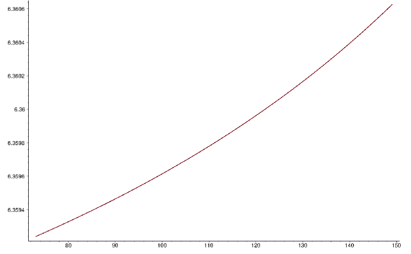
$R_{0}^{T}\in[6.3592,6.3607]$ vs $\beta^{G}\in[70,150]$

Figure 3: $R_{0}^{T}$ when varying $\beta^{A}$, $\beta^{C}$ and $\beta^{G}$, respectively.

The variation of $\beta^{A}$ has also a significative impact on the community and the host country, namely, in the number of infected and infectious individuals after $5$ years, see Fig. 4. Defining $I_{X}(t,s)=\left.I_{C}(t)\right|_{\beta^{A}=s}$ with $X\in\{C,G\}$, we have

$$\frac{I_{C}(5,180)}{I_{C}(5,150)}\approx 1.24,\quad\frac{I_{C}(5,120)}{I_{C}(5,150)}\approx 0.70,\quad\frac{I_{G}(5,180)}{I_{G}(5,150)}\approx 1.20,\quad\frac{I_{G}(5,120)}{I_{G}(5,150)}\approx 0.77.$$

An increase (decrease) of $20\%$ in $\beta^{A}$ implies a 5 years increase of approximately $20\%$ (decrease of $30\%$) in $I_{C}$ and $I_{G}$, respectively. This enforce the importance of additional effort to treat TB in countries with high TB incidence, not only because of their population health improvement, but also because of the implications on the health of individuals in other host countries.

$I_{C}(t)\in[0,0.0006]$ vs $t\in[0,5]$

$I_{G}(t)\in[0,0.0004]$ vs $t\in[0,5]$

Figure 4: $I_{C}(t)$ and $I_{G}(t)$ when varying $\beta^{A}$ (box: $\beta^{A}=120$, solid: $\beta^{A}=150$, cross: $\beta^{A}=180$).

3.1.2 Variation in the transfer of individuals (i.e., changing $a^{A}$ and $a^{B}$)

The transfer of individuals between (A) and (C)+(G) (i.e., (B)) is determined by the functions $\gamma_{A}(t)$ and $\gamma_{B}(t)$, which are here assumed to be equal to the parameters $a^{A}$ and $a^{B}$. From Fig. 5 it is clear, as expected, that an increment on the flux of individuals moving from areas of lower TB incidence to areas of higher TB incidence reduces $R_{0}^{T}$ and, on the contrary, an increment in the flux of individuals moving from areas of high TB incidence to areas of lower TB incidence increases $R_{0}^{T}$. Note that $R_{0}^{T}$ grows very fast for smaller values of $a^{A}$ and then tends to stabilize with the flux of persons coming from the high incidence TB area.

An interesting phenomena when varying $a^{A}$ appears in the variable $I_{G}$, i.e., the number of infected individuals in (G) (the community), see Fig. 6. It tells us that it is better for the community to have some moderate exchange of persons with the high incidence TB region. Such behavior and its reverse, after some time, seems to be related to the chosen value of $\zeta$ (discussed in the next subsection). It also imply that a careful study of the seasonality distribution of persons traveling between (A) and (B) may be more relevant for (G) than expected a priori. On the host country viewpoint, such phenomena is not noticed as one can see from the evolution of the total number of infected individuals in the host country, i.e., $I_{C}(t)\,N_{C}(t)+I_{G}\,N_{G}(t)$, see Fig. 6.

$R_{0}^{T}\in[6.3,6.7]$ vs $a^{A}\in[0,0.1]$

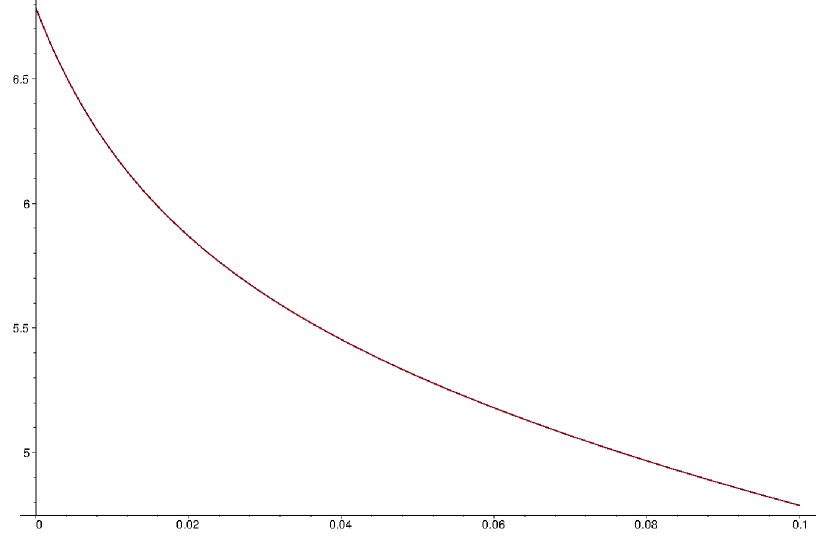
$R_{0}^{T}\in[4.8,6.8]$ vs $a^{B}\in[0,0.1]$

Figure 5: $R_{0}^{T}$ when varying $a^{A}$ and $a^{B}$, respectively.

$I_{G}(t)\in[0,0.0008]$ vs $t\in[0,5]$

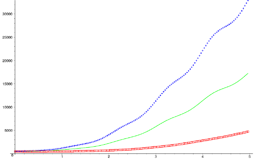
$\mathcal{N}\in[0,35000]$ vs $t\in[0,5]$

Figure 6: $I_{G}(t)$ and total number $\mathcal{N}$ of infected individuals in $(C)+(G)$ when varying $a^{A}$ (box: $a^{A}=0$, solid: $a^{A}=0.05$, cross: $a^{A}=0.1$).

3.1.3 About the ratio of individuals that stay in the community versus spread in the host country (i.e., changing $\zeta$)

In what follows we analyze the impact of the existence of a community of immigrants coming from a high incidence TB area on the host country, the country of origin and in the global situation. Recall that $\zeta$ is the percentage of persons traveling that come/go specifically to (G) versus the complementary (C). Hence, the situation $\zeta=0$ means that all persons traveling between Angola and Portugal all come/go to (C) and none to (G). On the contrary, $\zeta=1$ means that all persons traveling between Angola and Portugal all come/go to (G). From the analysis of Fig. 7 (right), it is clear that the existence of a community of immigrants coming from a high incidence TB area is convenient for the host country in order to better control TB spread. Regarding the point of view of Angola, a change in $\zeta$ is not significative as one can see, in Table 3, that $I_{A}$ is not affected by a change in $\zeta$.

On a global viewpoint, a change in $\zeta$ has a big impact on the reproduction number $R_{0}^{T}$, see Fig. 7 (left), for which the existence of communities turn to be also convenient. In fact, the function attains a minimum value that can be estimated from the approximated fitting by a parabolic function as

$$R_{0}(T)=$6.383321621$+ˆ’$0.114757045$x+$0.121874753$x^{2},$$

see Table 2. Hence, we may say that the optimal value for $\zeta$ is approximately

$$\min_{0\leq\zeta\leq 1}R_{0}^{T}(\zeta)=\frac{$0.114757045$}{2\times$0.121874753$}\approx 0.46.$$

$R_{0}^{T}\in[6.35,6.39]$ vs $\zeta\in[0,1]$

$\mathcal{H}(t)\in[0,7500]$ vs $t\in[0,5]$

Figure 7: $R_{0}^{T}$ versus $\zeta$ and total number $\mathcal{H}(t)=I_{C}(t)\,N_{C}(t)+I_{G}(t)\,N_{G}(t)$ of infected individuals in the host country versus $t$ when changing $\zeta$ (box: $\zeta=0$; solid: $\zeta=0.5$; cross: $\zeta=1$).

4 Numerical results and discussion

Regarding the sensitivity analysis, we numerically simulated the system (2.8)–(2.11) by considering all parameters fixed except one chosen parameter for which we consider three possible values according with

$$\begin{array}[]{ll}\beta^{A}\in\left\{150(1-\theta),150,150(1+\theta)\right\},&\beta^{C}\in\left\{72.358(1-\theta),72.358,72.358(1+\theta)\right\},\\ \beta^{G}\in\left\{\beta^{C},\frac{\beta^{C}+\beta^{A}}{2},\beta^{A}\right\},&k^{C}\in\left\{0.87(1-\theta),0.87,0.87(1+\theta)\right\},\\ \phi_{T}^{G}\in\left\{\phi_{T}^{C},\frac{\phi_{T}^{C}+\phi_{T}^{A}}{2},\phi_{T}^{A}\right\},&a^{A}\in\left\{0,0.05,0.1\right\},\\ a^{B}\in\left\{0,0.05,0.1\right\},&\zeta\in\left\{0,0.5,1\right\},\\ \end{array}$$

where $\theta=0.2$ (i.e., a variation of $\pm 20\%$). The middle levels are the values considered when the parameters are fixed.

$L_{A}(t)\in[0.35,0.66]$ vs $t\in[0,5]$

$I_{G}(t)\in[0,0.0006]$ vs $t\in[0,5]$

Figure 8: $L_{A}(t)$ when varying $\beta^{A}$ and $I_{G}(t)$ when varying $\zeta$ (box: smaller level, solid: middle level, cross: higher level).

Considering that system (2.8)–(2.11) has $15$ relevant state-space variables and we are perturbing $8$ parameters (with $3$ levels), even with overlapping of the levels on the same graphic, such analysis implies the study of $360$ functions aggregated in $120$ graphics. We want to quantify and describe the qualitative behavior and difference between the evolutions, when comparing the different levels. Additionally, a direct visual interpretation of the plots may be biased since the plots are not in the same scale, which may give a quite erroneous filling of disparity between functions when, in fact, the difference may be in a small amount, e.g., see Fig. 8. To deal with such issues, in a precise and normalized way, we considered the following procedure.

Let $F_{Y,P,1}(t),F_{Y,P,2}(t),F_{Y,P,3}(t)$ be the evolution functions associated to one of the state-variables

$$Y\in\{S_{A},S_{C},S_{G},P_{A},P_{C},P_{G},I_{A},I_{C},I_{G},L_{A},L_{C},L_{G},T_{A},T_{C},T_{G}\}$$

and to one of the three variation levels of a parameter $P\in\{\beta^{A},\beta^{C},\beta^{G},k^{C},\phi_{T}^{G},a^{A},a^{B},\zeta\}$. Let $\mathcal{T}>0$ denote the total time of simulation. Define

$$\vartheta(t)=\frac{1}{2}\left(\max_{i\in\mathcal{L}}{F_{Y,P,i}(t)}+\min_{i\in\mathcal{L}}{F_{Y,P,i}(t)}\right)\quad\mbox{ and }\quad\varrho(t)=\frac{1}{4}\left(\max_{i\in\mathcal{L}}{F_{Y,P,i}(t)}-\min_{i\in\mathcal{L}}{F_{Y,P,i}(t)}\right)^{2}$$

for $t\in[0,\mathcal{T}]$ and $\mathcal{L}=\{1,2,3\}$. We divide the analysis of the graphics, like in Fig. 8, in three regions of time: beginning for $t\in\mathcal{B}=[0,\frac{1}{3}\mathcal{T}]$; middle when $t\in\mathcal{M}=[\frac{1}{3}\mathcal{T},\frac{2}{3}\mathcal{T}]$; and end when $t\in\mathcal{E}=[\frac{2}{3}\mathcal{T},\mathcal{T}]$. The time set for the complete graph is denoted by $\mathcal{A}=[0,\mathcal{T}]$. Hence, we define

$$\xi_{\mathcal{S}}=\frac{\int_{\mathcal{S}}\varrho(s)\,ds}{\int_{0}^{\mathcal{T}}\vartheta(s)\,ds}\>\mbox{ with }\>\mathcal{S}\in\left\{\mathcal{B},\mathcal{M},\mathcal{E}\right\}.$$

It is clear, from the linearity of the integral, that $\xi_{\mathcal{A}}=\xi_{\mathcal{B}}+\xi_{\mathcal{M}}+\xi_{\mathcal{E}}$. To understand what $\xi_{\mathcal{A}}$ measures, consider the hypothetical situation where $F_{Y,P,1}(t)\equiv m+\theta$, $F_{Y,P,2}(t)\equiv m$, and consider $F_{Y,P,3}(t)\equiv m-\theta$ for some $m\in\mathbb{R}$ and $\theta>0$. Then,

$$\varphi(t)\equiv m,\>\>\varrho(t)\equiv\theta^{2}\quad\Rightarrow\quad\xi_{\mathcal{A}}=\frac{\theta^{2}}{m}.$$

So, although different, $\xi_{\mathcal{A}}$ is somehow similar to the variance over the average, which gives an indication of how much the functions are spread from the average value (between them in each instant of time). The definition of $\xi_{\mathcal{A}}$ is also invariant to scale factors, which is quite useful to eliminate erroneous interpretations of graphics, that may happen without such measuring tools.

For the qualitative description of the variability of the evolution functions, we introduced the following tagging notation based on concrete specifications:

• (cases $\mathcal{A}_{--}$, $\mathcal{A}_{+-}$, $\mathcal{A}_{++}$) if $\max(\xi_{\mathcal{B}},\xi_{\mathcal{M}},\xi_{\mathcal{E}})<0.4$;

• (cases $\mathcal{B}_{--}$, $\mathcal{B}_{+-}$, $\mathcal{B}_{++}$) if $\mathcal{S}\neq\mathcal{A}$ and $\max(\xi_{\mathcal{B}},\xi_{\mathcal{M}},\xi_{\mathcal{E}})=\xi_{\mathcal{B}}$;

• (case $\mathcal{M}_{--}$, $\mathcal{M}_{+-}$, $\mathcal{M}_{++}$) if $\mathcal{S}\neq\mathcal{A}$ and $\max(\xi_{\mathcal{B}},\xi_{\mathcal{M}},\xi_{\mathcal{E}})=\xi_{\mathcal{M}}$;

• (cases $\mathcal{E}_{--}$, $\mathcal{E}_{+-}$, $\mathcal{E}_{++}$) if $\mathcal{S}\neq\mathcal{A}$ and $\max(\xi_{\mathcal{B}},\xi_{\mathcal{M}},\xi_{\mathcal{E}})=\xi_{\mathcal{E}}$;

• (cases $\mathcal{S}_{--}$ with $\mathcal{S}\in\left\{\mathcal{B},\mathcal{M},\mathcal{E},\mathcal{A}\right\}$) if $\xi_{\mathcal{A}}<0.01$;

• (cases $\mathcal{S}_{+-}$ with $\mathcal{S}\in\left\{\mathcal{B},\mathcal{M},\mathcal{E},\mathcal{A}\right\}$) if it is not $\mathcal{S}_{--}$ and $\xi_{\mathcal{A}}<0.25$;

• (cases $\mathcal{S}_{+-}$ with $\mathcal{S}\in\left\{\mathcal{B},\mathcal{M},\mathcal{E},\mathcal{A}\right\}$) if it is not $\mathcal{S}_{--}$ and $\mathcal{S}_{+-}$.

If $\xi_{\mathcal{A}}<0.1$, then we consider that the variation is not numerically significative, so it is not discussed. Table 3 resumes the sensitivity analysis, where the only tag behaviors that appear are $\mathcal{B}_{+-}$, $\mathcal{M}_{+-}$, $\mathcal{E}_{+-}$, and $\mathcal{E}_{++}$.

	$\mathcal{B}_{+-}$	$\mathcal{M}_{+-}$	$\mathcal{E}_{+-}$	$\mathcal{E}_{++}$	$\xi_{\mathcal{A}}$ values, respectively
$S_{A}$	$a^{B}$	$\beta^{A}$			$$1.1710-01$,$2.6410-01$$
$P_{A}$			$a^{B}$	$\beta^{A}$	$$2.3410-01$,$3.7910-01$$
$I_{A}$			$a^{B}$	$\beta^{A}$	$$2.2810-01$,$4.2310-01$$
$L_{A}$			$\beta^{A}$		$1.2610-01$
$T_{A}$			$a^{B}$	$\beta^{A}$	$$2.1810-01$,$4.5810-01$$
$S_{C}$			$a^{A}$		$1.3310-01$
$P_{C}$			$k^{C},a^{B}$	$\beta^{A},\beta^{C},a^{A},\zeta$	$$2.4710-01$,$1.8210-01$,$3.7810-01$,$2.8410-01$,$8.4310-01$,$1$$
$I_{C}$			$\beta^{C},k^{C},a^{B}$	$\beta^{A},a^{A},\zeta$	$$1.8110-01$,$3.7210-01$,$1.8410-01$,$3.7610-01$,$8.7210-01$,$9.8710-01$$
$L_{C}$			$a^{A}$		$2.4310-01$
$T_{C}$			$\beta^{C},a^{B}$	$\beta^{A},a^{A},\zeta$	$$1.3910-01$,$1.7310-01$,$3.9710-01$,$9.2810-01$,$9.7410-01$$
$S_{G}$		$a^{A}$		$\zeta$	$$3.9510-01$,$2.8810-01$$
$P_{G}$			$\beta^{A},\phi_{T}^{G},a^{A}$	$\beta^{G},k^{C},\zeta$	$$1.8010-01$,$1.5410-01$,$2.2610-01$,$7.6410-01$,$4.2110-01$,$3.9010-01$$
$I_{G}$			$\beta^{A},\beta^{G},\phi_{T}^{G},\zeta$	$k^{C},a^{A}$	$$1.9710-01$,$6.5310-01$,$1.9710-01$,$2.1510-01$,$5.1510-01$,$3.7510-01$$
$L_{G}$		$a^{A}$	$\beta^{G}$	$\zeta$	$$2.3810-01$,$9.4610-02$,$2.5910-01$$
$T_{G}$			$\beta^{A},\phi_{T}^{G}$	$k^{C},a^{A},\zeta$	$$2.0210-01$,$1.7210-01$,$2.8210-01$,$4.5610-01$,$1.9410-01$$

Table 3: Qualitative sensitivity analysis.

Table 3 is quite explanatory and shows relations between parameter perturbations and epidemiological compartments, in a mathematically precise and rather simple visual representation way. The variation of some parameters just gives the expected behavior, which shows that the proposed model is suitable for the situation under study. On the other hand, it also shows that some parameters that a priori we do not give much attention, as the distribution of persons between (G) and (C) (i.e., $\zeta$), play an important role in TB spread.

5 Conclusions

In this paper, we propose and analyze a new mathematical model for TB transmission that considers internal transfer of individuals. As a case-study, we consider a situation with three populations, namely, Angola (a country with high TB incidence), people living in a semi-closed community of Angola natives, and other persons living in Portugal (a country with low TB incidence). Each of the previous subsystems is divided into five epidemiological categories, which follow the TB transmission dynamics found in [13].

For the analysis and verification of the results presented in this paper, we developed a software tool, so-called sDL [42], that combines in the same framework the power of pre-processing systems (as m4 [12] and cpp [31]), a logical verification tool for classical and hybrid systems (as SMT [41] or KeYmaera [18]), a computer algebra system (as Maple [14]), and a numerical computing language (as Matlab [22]). The pre-processing systems allow the existence of a unique and general file, where constants and ODEs are defined in two hierarchical levels, in order to be used across all tools. The verification tool and the computer algebra system allowed to test the validity of some assumptions and verify the correctness of analytic/algebraic formulae. As expected, the numerical computing language allowed to do the numeric simulations and generate the corresponding graphics. Considering the potential of the software tool sDL, in a forthcoming publication, we intend to study real situations that are modeled by pure hybrid model systems, e.g., transmission coefficients that are discontinuous functions varying with climate and season conditions.

Simulations and sensitivity analysis show that variations of the transmission coefficient on the origin country has a big influence on the number of infected (and infectious) individuals on the community and the host country. This enforce the importance of an additional effort to treat TB and improve health conditions in countries with high TB incidence, since they remarkably affect (in long term) the health of individuals on other countries. As expected, an increment on the flux of individuals moving from areas of lower TB incidence to areas of higher TB incidence reduces the global reproduction number and an increment in the flux of individuals moving from areas of high TB incidence to areas of lower TB incidence increases the global reproduction number, but also introduce modifications in the evolution of each disease category that is not linearly proportional to flux rate. From the community point of view, it is better to have some moderate exchange of persons with the high incidence TB region. Seasonality distribution of persons traveling between Angola and Portugal has an important impact in the number of infected (and infectious) individuals in the community.

The main conclusion is that, contrary to some beliefs, the existence of a community of immigrants coming from a high incidence TB area seems to be convenient in a global point of view, as well as for the host country, in order to better control TB spread. On the other hand, it does not affect the TB incidence in the origin country of the immigrant community. By nonexistence of the community of immigrants we mean the situation where the individuals traveling are spread uniformly on the host country. As shown above, a key parameter in such analysis is the percentage of persons traveling from the high incidence TB area that will stay in the community. Such parameter has an optimal value for TB control, in the sense of minimizing the global reproduction number, that is near to $47\%$. The obtained results are valid under the hypothesis of a semi-closed community. Further studies are necessary for the situation without any flux restrictions.

Acknowledgments. Work partially supported by Portuguese funds through the Center for Research and Development in Mathematics and Applications (CIDMA) and the Portuguese Foundation for Science and Technology (FCT), within project UID/MAT/04106/2013. Rocha is also supported by the FCT project “DALI – Dynamic logics for cyber-physical systems: towards contract based design” with reference P2020-PTDC/EEI-CTP/4836/2014; Silva by the FCT post-doc fellowship SFRH/BPD/72061/2010; Silva and Torres by project TOCCATA, reference PTDC/EEI-AUT/2933/2014, funded by Project 3599 – Promover a Produção Científica e Desenvolvimento Tecnológico e a Constituição de Redes Temáticas (3599-PPCDT) and FEDER funds through COMPETE 2020, Programa Operacional Competitividade e Internacionalização (POCI), and by national funds through FCT. The authors are grateful to two referees for useful comments and suggestions.

References

[1]S. Blower, P. Small and P. Hopewell,
Control strategies for tuberculosis epidemics: New
models for old problems,
Science, 273 (1996), 497–500.
[2]F. Brauer and P. van den Driessche,
Models for transmission of disease with immigration of infectives,
Mathematical Biosciences 171 (2001), 143–154.
[3]C. Castillo-Chavez and Z. Feng,
Mathematical models for the disease dynamics of tuberculosis,
in Advances in Mathematical Population Dynamics-Molecules, Cells and Man
(eds. Mary Ann Horn, G. Simonett and G. Webb), Vanderbilt University Press, 1998, 117–128.
[4]T. Cohen and M. Murray,
Modeling epidemics of multidrug-resistant
M. tuberculosis of heterogeneous fitness,
Nat. Med. 10 (2004), no. 10, 1117–1121.
[5]M. G. M. Gomes, R. Aguas, J. S. Lopes, M. C. Nunes,
C. Rebelo, P. Rodrigues and C. J. Struchiner,
How host heterogeneity governs tuberculosis reinfection,
Proc. R. Soc. B 279 (2012), 2473–2478.
[6]M. G. M. Gomes, P. Rodrigues, F. M. Hilker, N. B. Mantilla-Beniers,
M. Muehlen, A. C. Paulo, G. F. Medley,
Implications of partial immunity on the prospects
for tuberculosis control by post-exposure interventions,
J. Theoret. Biol. 248 (2007), no. 4, 608–617.
[7]H. Hethcote,
A thousand and one epidemic models.
In: Levin, S.A. (ed.)
Frontiers in Theoretical Biology, pp. 504–515.
Springer, Berlin, 1994.
[8]H. Hethcote,
The mathematics of infectiuos diseases.
SIAM Rev. 42 (2000), 599–653.
[9]INE,
Resident Population Projections 2012–2060,
Statistics Portugal, 2014.
[10]IOM,
Migration & Tuberculosis: A pressing issue,
International Organization for Migration, 2012.
[11]Z-W. Jia, G-Y. Tang, Z. Jin, C. Dye,
S.J. Vlas, X-W. Lig, D. Feng, L-Q. Fang, W-J. Zhao and W-C. Cao,
Modeling the impact of immigration on the epidemiology of tuberculosis,
Theoretical Population Biology 73 (2008), 437–448.
[12]B. W. Kernighan and D. M. Ritchie,
The M4 macro processor,
Technical report, Bell Laboratories, Murray Hill, New Jersey, USA, 1977.
[13]J. S. Lopes, P. Rodrigues, S. T. R. Pinho,
R. F. S. Andrade, R. Duarte and M. G. M. Gomes,
Interpreting measures of tuberculosis transmission:
A case study on the Portuguese population,
BMC Infectious Diseases 14 (2014), no. 340, 9 pp.
[14]S. Lynch,
Dynamical systems with applications using MapleTM,
second edition, Birkhäuser Boston, Boston, MA, 2010.
[15]M. F. Mendes, J. R. Santos and C. Rego,
Imigrantes Angolanos em Portugal: breve caracterização
e contributos para a dinâmica populacional,
XI Congresso Luso Afro Brasileiro de Ciêcias Sociais, 2011.
[16]OECD,
International Migration Outlook 2014,
Organization for Economic Co-operation and Development, 2014.
[17]ONDR,
10o Relatório, Panorama das Doenças Respiratórias em Portugal,
Observatório Nacional das Doenças Respiratórias em Portugal, 2014–2015.
[18]A. Platzer,
Logical analysis of hybrid systems: Proving theorems for complex dynamics,
Springer, Berlin, 2010.
[19]RILP,
Migrações,
Revista Internacional em Língua Portuguesa,
III Série no. 24, 2011.
[20]P. Rodrigues, C. J. Silva and D. F. M. Torres,
Cost-effectiveness analysis of optimal control measures for tuberculosis,
Bull. Math. Biol. 76 (2014), no. 10, 2627–2645.
arXiv:1409.3496
[21]SEF,
Relatório de Imigração Fronteiras e Asilo,
Serviço de Estrangeiros e Fronteiras, 2013.
[22]M. Shahin,
Explorations of mathematical models in biology with MATLAB®,
Wiley, Hoboken, NJ, 2014.
[23]C. J. Silva and D. F. M. Torres,
Optimal control strategies for tuberculosis treatment: a case study in Angola,
Numer. Algebra Control Optim. 2 (2012), no. 3, 601–617.
arXiv:1203.3255
[24]C. J. Silva and D. F. M. Torres,
Optimal control for a tuberculosis model
with reinfection and post-exposure interventions,
Math. Biosci. 244 (2013), no. 2, 154–164.
arXiv:1305.2145
[25]K. Styblo,
Epidemiology of tuberculosis:
Epidemiology of tuberculosis in HIV prevalent countries,
Royal Netherlands Tuberculosis Association, 1991.
[26]P. van den Driessche and J. Watmough,
TReproduction numbers and sub-threshold endemic equilibria
for compartmental models of disease transmission,
Mathematical Biosciences 180 (2002), 29–48.
[27]E. Vynnycky and P. E. Fine,
The natural history of tuberculosis: the implications of
age-dependent risks of disease and the role of reinfection,
Epidemiol Infect. 119 (1997), no. 2, 183–201.
[28]C. L. Wesley and L. J. S. Allen,
The basic reproduction number in epidemic models with periodic demographics,
J. Biol. Dyn. 3 (2009), no. 2-3, 116–129.
[29]WHO,
Global Tuberculosis Control, WHO report 2013,
Geneva, Switzerland.
[30]WHO,
Global tuberculosis report 2014,
Geneva, World Health Organization, 2014.
[31]L. Wirzenius,
C preprocessor trick for implementing similar data types,
http://liw.iki.fi/liw/texts/cpp-trick.html
[32]J.H. Wolleswinkel-van den Bosch, N.J.D. Nagelkerke, J.F. Broekmans, M.W. Borgdorff,
The impact of immigration on the elimination of tuberculosis in The Netherlands: a model based approach,
Int. J. Tuberc. Lung Dis. 6 (2002), no. 2, 130–136.
[33]Y. Zhou, K. Khan, Z. Feng, J. Wu,
Projection of tuberculosis incidence with increasing immigration trends,
Journal of Theoretical Biology 254 (2008), 215–228.