Abstract

The laws of thermodynamics in the expanding universe are formulated within the quasi-metric framework. Since the quasi-metric cosmic expansion does not directly influence momenta of material particles, so that the expansion directly cools the photons only (or more generally, null particles), these laws differ substantially from their counterparts in standard cosmology. An approximate model describing thermodynamics during neutrino decoupling is set up. This model yields, assuming that no neutrino mass eigenstate is null so that the expansion does not directly cool the neutrinos, that the result after neutrino decoupling will be a non-thermal relic neutrino background which decoupled gradually over about 20-30 years when the photon plasma had a temperature of ${\sim}{\rm 100-50{\ }keV}/k_{\rm B}$. The relic neutrinos are predicted to have a number density today more than twice the standard cosmology result and to have the same energy distribution today as they had just after decoupling. As a consequence of this, the relic neutrino background is predicted to consist of neutrino mass eigenstates with an average energy of ${\sim}{\rm 170{\ }keV}$. This predicted relic neutrino background is strongly inconsistent with detection rates measured in solar neutrino detectors (Borexino in particular), unless some particular property of neutrinos makes the relic neutrino background essentially undetectable (e.g., if one neutrino mass eigenstate is null and the two massive mass eigenstates decay into the the null eigenstate over cosmic time scales). But in the absence of such a natural explanation from neutrino physics, the current status of quasi-metric relativity has been changed to non-viable.

1 Introduction

Nowadays one often hears the assertion that the science of cosmology has matured to the point where one speaks of “precision cosmology”, meaning that its theoretical foundations are considered beyond reasonable doubt and that almost all cosmological data are consistent with the standard big bang (SBB) scenario (currently characterized by a positive cosmological constant and cold dark matter) based on general relativity (GR). Reasons for this view are based on analyses of the cosmic microwave background (CMB) and moreover on the predictions coming from standard big bang nucleosynthesis (SBBN) agreeing well with the observed abundances of light elements, so that together with results coming from other cosmological observations, the values of the cosmological parameters can be inferred in a consistent way. In particular the successes of SBBN are convincing since its predictions are overconstrained and not a result of mere parameter-fitting exercises.

However, mainstream cosmology is based on GR, so the successes of the SBB scenario cannot be independent of how well GR fares on smaller scales. Unfortunately, GR has difficulties explaining galactic phenomenology such as rotation curve shapes without doing more than essentially fitting suitable dark matter distributions to give the desired results. Moreover, the physics behind observed scaling relations such as the Tully-Fisher relation has no obvious theoretical basis in GR (or in Newtonian gravity) whatsoever. Even on such a small scale as the solar system there are anomalies not well explained by GR (or Newtonian gravity). But some of these anomalies have simple explanations based on first principles coming from an alternative space-time framework, the so-called quasi-metric framework (QMF) [1, 2]. Said explanations are mostly based on the most characteristic feature of the QMF, namely that the cosmic expansion is postulated to be independent of space-time’s causal structure. As a consequence, the QMF predicts that the cosmic expansion should be detectable in the solar system, and that this naturally explains several anomalies [3]. This means that there is observational support for the possibility that GR mismodels the cosmic expansion, so that some of the fundamental assumptions underlying the SBB scenario could be false. This indicates that the SBB scenario may not be very robust after all and that any talk of “precision cosmology” would be premature.

But even if the QMF is able to explain some solar system anomalies in addition to the usual gravitational solar system tests, it has not yet been shown to be viable in general. One step towards viability would be to show that the predicted thermodynamics of the early Universe is consistent with current observational results. This goal motivates further exploration of quasi-metric cosmology and the question of its viability, which is the theme of the present paper. However, as we shall see, the results are not promising since the properties of the predicted cosmic neutrino background are in violent conflict with observations.

In short, the crucial point is that in the QMF, the momenta of material particles are not directly affected by the cosmic expansion. This is a unique feature of the QMF and as a consequence, thermodynamics in the expanding universe as described within the QMF, is nonstandard. This results in the specific prediction that there should at present exist a non-thermal relic cosmological neutrino background in the form of neutrino mass eigenstates, with average energy of $\sim$ 170 keV. Unless some exotic properties of neutrinos make the relic neutrino background essentially unobservable (e.g., if one neutrino mass eigenstate is null and the two massive mass eigenstates decay into the the null eigenstate over cosmic time scales), said prediction is in violent conflict with measured results from solar neutrino observatories such as SAGE, GALLEX/GNO and Borexino. In view of this result the status of the QMF has been changed to not viable.

2 Motivating quasi-metric relativity

The quasi-metric space-time framework (QMF), along with motivations for introducing it, has been published in [1]. A synopsis is presented in the present paper for the benefit of new readers.

The main motivation for inventing the QMF is of a very general philosophical nature. That is, traditional field theories consist of two independent parts; field equations and initial conditions. This form ensures that field theories can in principle be generally applied to all systems within their domain of validity. But for cosmology this flexibility is a liability; since the Universe is unique, it is impossible in principle to have observational knowledge of alternatives to cosmic initial conditions, global evolution and structure. Any diversity of such possibilities represents a serious limitation to what can be known in principle, and should be avoided if possible. That is, since the Universe is observationally unique, so should the nature of its global evolution be.

It turns out that, to construct a general framework fulfilling this requirement, one is pretty much led to the QMF. Moreover, the QMF accomplishes this requirement by describing the global cosmic expansion as an absolute, prior-geometric phenomenon, not being part of space-time’s causal structure. In this way the cosmic expansion does not depend on field equations and initial conditions, meaning that the Universe is not described as a purely dynamical system.

Similar to the Robertson-Walker (RW) models in GR, the cosmic expansion in the QMF is defined by means of a family of “preferred” observers, the so-called fundamental observers (FOs). A further similarity with the RW-models is the existence of a global time function $t$, such that $t$ splits up space-time into a “distinguished” set of spatial hypersurfaces, the so-called fundamental hypersurfaces (FHSs). But since the cosmic expansion in the QMF by hypothesis is not part of space-time’s causal structure, $t$ cannot be an ordinary time coordinate on a Lorentzian manifold. Rather, it should play the role of an independent evolution parameter, parametrizing any change in the space-time geometry that has to do with the cosmic expansion. On the other hand, space-time must also be equipped with a causal structure in the form of a Lorentzian manifold. This Lorentzian manifold must also accommodate the FOs and the FHSs, which means that its topology should allow the existence of a global ordinary time coordinate $x^{0}$. (Note that, to ensure the uniqueness of this construction, the FHSs must be compact.)

Taking into account the above considerations, the geometrical basis of the QMF can now be defined. That is, the geometry underlying the QMF consists of a 5-dimensional differentiable manifold with topology ${\cal M}{\times}{\bf R}_{1}$, where ${\cal M}={\cal S}{\times}{\bf R}_{2}$ is a Lorentzian space-time manifold, ${\bf R}_{1}$ and ${\bf R}_{2}$ both denote the real line and ${\cal S}$ is a compact 3-dimensional manifold (without boundaries). That is, in addition to the usual time dimension and 3 space dimensions there is an extra degenerate time dimension ${\bf R}_{1}$ represented by the global time function $t$. Moreover, the manifold ${\cal M}{\times}{\bf R}_{1}$ is equipped with two 5-dimensional degenerate metrics ${\bf{\bar{g}}}_{t}$ and ${\bf g}_{t}$, where the degeneracies are described by the conditions ${\bf{\bar{g}}}_{t}({\frac{\partial}{{\partial}t}},{\cdot}){\equiv}0$ and ${\bf g}_{t}({\frac{\partial}{{\partial}t}},{\cdot}){\equiv}0$, respectively. The metric ${\bf{\bar{g}}}_{t}$ is coupled to matter fields via field equations, and from this on can construct the “physical” metric ${\bf g}_{t}$ used when comparing predictions to experiments. Note that these metrics have the property that the FOs always move orthogonally to the FHSs.

To reduce space-time to 4 dimensions, one obtains the quasi-metric space-time manifold $\cal N$ by slicing the submanifold determined by the equation $x^{0}=ct$ out of the 5-dimensional differentiable manifold ${\cal M}{\times}{\bf R}_{1}$. It is essential that this slicing is unique since the two global time coordinates should be physically equivalent; the only reason to separate between them is that they are designed to parameterize fundamentally different physical phenomena. Since the geometric structure on ${\cal N}$ is inherited from that on ${\cal M}{\times}{\bf R}_{1}$ just by restricting the fields to ${\cal N}$ (no projections), the 5-dimensional degenerate metric fields ${\bf{\bar{g}}}_{t}$ and ${\bf g}_{t}$ may be regarded as one-parameter families of Lorentzian 4-metrics on $\cal N$ (this terminology is merely a matter of semantics). Note that there exists a set of particular coordinate systems especially well adapted to the geometrical structure of quasi-metric space-time, the global time coordinate systems (GTCSs). A coordinate system is a GTCS iff the time coordinate $x^{0}$ is related to $t$ via $x^{0}=ct$ in ${\cal N}$.

Since the role of $t$ is to describe how the cosmic expansion directly influences space-time geometry, $t$ should enter ${\bf{\bar{g}}}_{t}$ and ${\bf g}_{t}$ explicitly as a scale factor. However, unlike its counterpart in the RW-models, this scale factor cannot be calculated from dynamical equations, but must be an “absolute” quantity. Since the form of the scale factor should not introduce any extra arbitary scale or parameter, the only possibile option for a scale factor with the dimension of length is to set it equal to $ct$. This scale factor may be multiplied by a second, dimensionless scale factor taking into account the effects of gravity. But since the geometry of the FHSs in $({\cal N},{\bf{\bar{g}}}_{t})$ is postulated to represent a measure of gravitational scales in terms of atomic units, any extra dimensionless scale factor should enter ${\bf{\bar{g}}}_{t}$ as a conformal factor.

Furthermore, since there is no reason to introduce any nontrivial spatial topology, the global basic geometry of the FHSs (neglecting the effects of gravity) should be that of the 3-sphere ${\bf S^{3}}$. To fulfil the above said requirements and to avoid that this fixation of the spatial geometry interferes with the dynamics of ${\bf{\bar{g}}}_{t}$, it should take a restricted form. It then turns out that the most general form of ${\bf{\bar{g}}}_{t}$ (expressed in an isotropic GTCS) can be written as the family of line elements (using Einstein’s summation convention)

$${\overline{ds}}^{2}_{t}={\bar{N}}_{t}^{2}{\Big{\{}}-{\Big{[}}1-{\bar{N}}^{i}{\bar{N}}^{j}S_{ij}{\Big{]}}(dx^{0})^{2}+2{\frac{t}{t_{0}}}{\bar{N}}^{i}S_{ij}dx^{j}dx^{0}+{\frac{t^{2}}{t_{0}^{2}}}S_{ij}dx^{i}dx^{j}{\Big{\}}},$$ (1)

where $t_{0}$ is an arbitrary reference epoch, ${\bar{N}}_{t}$ is the lapse function family, ${\frac{t}{t_{0}}}{\bar{N}}^{i}{\frac{\partial}{{\partial}x^{i}}}$ is the family of shift vector fields and where $S_{ij}dx^{i}dx^{j}$ is the metric of ${\bf S^{3}}$ (with radius equal to $ct_{0}$). The affine structure constructed on ${\cal M}{\times}{\bf R}_{1}$ (see below) limits any possible $t$-dependence of the quantities present in equation (1). Specifically, ${\bar{N}}_{t}$ may depend explicitly on $t$, whereas ${\bar{N}}^{i}$ may not.

Next, $({\cal N},{\bf{\bar{g}}}_{t})$ and $({\cal N},{\bf g}_{t})$ are equipped with linear and symmetric connections      and     , respectively. These connections are identified with the usual Levi-Civita connection for constant $t$, yielding the standard form of the connection coefficients not containing $t$. The rest of the connection coefficients are determined by the requirements

$${\begin{picture}(2.0,0.0)(-1.0,-1.4)\put(0.0,0.0){\makebox(0.0,0.0)[]{$\bf{\bar{\nabla}}$}} \put(0.0,2.4){\makebox(0.0,0.0)[]{\mbox{\tiny$\star$}}} \end{picture}}_{\frac{\partial}{{\partial}t}}{\bf{\bar{g}}}_{t}=0,\qquad{\begin{picture}(2.0,0.0)(-1.0,-1.4)\put(0.0,0.0){\makebox(0.0,0.0)[]{$\bf{\bar{\nabla}}$}} \put(0.0,2.4){\makebox(0.0,0.0)[]{\mbox{\tiny$\star$}}} \end{picture}}_{\frac{\partial}{{\partial}t}}{\bf{\bar{n}}}_{t}=0,\qquad{\begin{picture}(2.0,0.0)(-1.0,-1.4)\put(0.0,0.0){\makebox(0.0,0.0)[]{$\bf{\nabla}$}} \put(0.0,2.4){\makebox(0.0,0.0)[]{\mbox{\tiny$\star$}}} \end{picture}}_{\frac{\partial}{{\partial}t}}{\bf g}_{t}=0,\qquad{\begin{picture}(2.0,0.0)(-1.0,-1.4)\put(0.0,0.0){\makebox(0.0,0.0)[]{$\bf{\nabla}$}} \put(0.0,2.4){\makebox(0.0,0.0)[]{\mbox{\tiny$\star$}}} \end{picture}}_{\frac{\partial}{{\partial}t}}{\bf n}_{t}=0,$$ (2)

where ${\bf{\bar{n}}}_{t}$ and ${\bf n}_{t}$ are families of unit normal vector fields to the FHSs in $({\cal N},{\bf{\bar{g}}}_{t})$ and $({\cal N},{\bf g}_{t})$, respectively. The requirements shown in equation (2) yield the nonzero extra connection coefficients (using a GTCS and where a comma denotes a partial derivative)

$${\begin{picture}(2.0,0.0)(-1.0,-1.4)\put(0.0,0.0){\makebox(0.0,0.0)[]{$\bar{\Gamma}$}} \put(0.0,2.4){\makebox(0.0,0.0)[]{\mbox{\tiny$\star$}}} \end{picture}}_{t0}^{{\,}0}={\frac{{\bar{N}}_{t,t}}{{\bar{N}}_{t}}},\qquad{\begin{picture}(2.0,0.0)(-1.0,-1.4)\put(0.0,0.0){\makebox(0.0,0.0)[]{$\bar{\Gamma}$}} \put(0.0,2.4){\makebox(0.0,0.0)[]{\mbox{\tiny$\star$}}} \end{picture}}_{tj}^{{\,}i}={\Big{(}}{\frac{1}{t}}+{\frac{{\bar{N}}_{t,t}}{{\bar{N}}_{t}}}{\Big{)}}{\delta}^{i}_{j},\qquad{\begin{picture}(2.0,0.0)(-1.0,-1.4)\put(0.0,0.0){\makebox(0.0,0.0)[]{$\Gamma$}} \put(0.0,2.4){\makebox(0.0,0.0)[]{\mbox{\tiny$\star$}}} \end{picture}}_{tj}^{{\,}i}={\frac{1}{t}}{\delta}^{i}_{j},$$ (3)

in addition to identical expressions for those obtained by permuting the two lower indices.

As mentioned earlier, the scale factor ${\bar{N}}_{t}ct$ of the FHSs as obtained from equation (1), is interpreted as a gravitational scale measured in atomic units. This interpretation must also hold for all dimensionful gravitational quantities with dimension of length to some power (here, time scales the same way as length and inversely of mass while charge is in effect dimensionless). In particular this applies to the gravitational coupling parameter $G_{t}$, effectively scaling as length squared. However, $G_{t}$ couples both to mass and to charge squared, so if one wants to transfer the variability of $G_{t}$ to matter sources, it will be necessary to define two gravitational constants $G^{\rm B}$ and $G^{\rm S}$. Here, $G^{\rm B}$ is the “bare” gravitational constant coupling to charge or more generally to the electromagnetic field and in principle measurable in local gravitational experiments at an arbitrary reference event epoch $t_{0}$. Moreover, $G^{\rm S}$ is the “screened” gravitational constant coupling to material matter fields and in principle also measurable in local gravitational experiments at the reference epoch $t_{0}$. This means that we must have non-universal gravitational coupling between matter sources and space-time geometry. The necessity of having non-universal gravitational coupling was missed in the original formulation of the QMF.

The variability of dimensionful gravitational quantities as measured in atomic units, in addition to transferring the variability of $G_{t}$ to matter sources, imply that one must distinguish between active mass measured dynamically as a source of gravity and passive mass, i.e., passive gravitational mass or inertial mass. (Similarly one must distinguish between active charge and passive charge.) Taking into account said variation of gravitational scales measured in atomic units, it is possible to set up local conservation laws in $({\cal N},{\bf{\bar{g}}}_{t})$ involving the covariant derivative ${\ }{\begin{picture}(2.0,0.0)(-1.0,-1.4)\put(0.0,0.0){\makebox(0.0,0.0)[]{$\bf{\bar{\nabla}}$}} \put(0.0,2.4){\makebox(0.0,0.0)[]{\mbox{\tiny$\star$}}} \end{picture}}{\ }{\bf{\cdot}}{\bf T}_{t}$ of the active stress-energy tensor ${\bf T}_{t}$. These local conservation laws do not depend on the nature of the source. In component notation, they take the form [1, 2]

$$T^{\nu}_{(t){\mu}{\bar{*}}{\nu}}{\equiv}c^{-1}T^{0}_{(t){\mu}{\bar{*}}t}+T^{\nu}_{(t){\mu};{\nu}},\quad T^{0}_{(t){\mu}{\bar{*}}t}=-{\frac{2}{{\bar{N}}_{t}}}{\Big{(}}{\frac{1}{t}}+{\frac{{\bar{N}}_{t,t}}{{\bar{N}}_{t}}}{\Big{)}}T_{(t){\bar{\perp}}{\mu}},\quad T^{\nu}_{(t){\mu};{\nu}}=2{\frac{{\bar{N}}_{t,{\nu}}}{{\bar{N}}_{t}}}T^{\nu}_{(t){\mu}},$$ (4)

where the symbol ’${\bar{*}}$’ denotes covariant derivative with      and where the symbol ’${\bar{\perp}}$’ denotes a scalar product with $-{\bf{\bar{n}}}_{t}$. The local conservation laws (4) imply that inertial test particles move along geodesics of      in $({\cal N},{\bf{\bar{g}}}_{t})$, and this ensures that inertial test particles move along geodesics of      in $({\cal N},{\bf g}_{t})$ as well [1, 2]. Note that due to equation (2), the lapse function $N$ of the FOs in $({\cal N},{\bf g}_{t})$ cannot depend explicitly on $t$. This means that, when making the transformation ${\bf{\bar{g}}}_{t}{\rightarrow}{\bf g}_{t}$, $N$ gets an “effective” time dependence parametrized by $x^{0}$. Then the equations of motion in $({\cal N},{\bf g}_{t})$ read (in a GTCS, in component notation)

$${\frac{d^{2}x^{\mu}}{d{\lambda}^{2}}}+{\Big{(}}{\begin{picture}(2.0,0.0)(-1.0,-1.4)\put(0.0,0.0){\makebox(0.0,0.0)[]{$\Gamma$}} \put(0.0,2.4){\makebox(0.0,0.0)[]{\mbox{\tiny$\star$}}} \end{picture}}_{t{\nu}}^{{\,}{\mu}}{\frac{dt}{d{\lambda}}}+{\begin{picture}(2.0,0.0)(-1.0,-1.4)\put(0.0,0.0){\makebox(0.0,0.0)[]{$\Gamma$}} \put(0.0,2.4){\makebox(0.0,0.0)[]{\mbox{\tiny$\star$}}} \end{picture}}_{{\beta}{\nu}}^{{\,}{\mu}}{\frac{dx^{\beta}}{d{\lambda}}}{\Big{)}}{\frac{dx^{\nu}}{d{\lambda}}}={\Big{(}}{\frac{d{\tau}_{t}}{d{\lambda}}}{\Big{)}}^{2}a_{(t)}^{\mu},$$ (5)

where $d{\tau}_{t}$ is the proper time interval as measured along the curve, ${\lambda}$ is some general affine parameter, and ${\bf a}_{t}$ is the 4-acceleration measured along the curve.

Due to the need for non-universal gravitational couplings, it is convenient to split up ${\bf T}_{t}$ into one electromagnetic part ${\bf T}_{t}^{\rm(EM)}$ and one part ${\bf T}_{t}^{\rm mat}$ representing matter fields. However, the restricted form (1) of ${\bf{\bar{g}}}_{t}$ implies that full couplings of ${\bf T}^{\rm(EM)}_{t}$ and ${\bf T}^{\rm mat}_{t}$ to space-time curvature cannot exist. Moreover, since the restrictions involve the spatial geometry only and since these restrictions should not affect the dynamics of ${\bf{\bar{g}}}_{t}$, the intrinsic curvature of the FHSs cannot couple explicitly to matter sources. Besides, only that part of the space-time curvature obtained by setting $t$ constant should couple to matter. Fortunately, it turns out that a (generalized) subset of the Einstein field equations can be tailored to ${\bf{\bar{g}}}_{t}$ so that partial couplings exist, having the desired properties. Setting $c^{-2}{\bar{a}}_{{\cal F}j}{\equiv}{\frac{{\bar{N}}_{t,j}}{{\bar{N}}_{t}}}$, this leads to the field equations (expressed in a GTCS)

$${\bar{R}}_{(t){\bar{\perp}}{\bar{\perp}}}=c^{-4}{\bar{a}}_{{\cal F}k}{\bar{a}}_{\cal F}^{k}+c^{-2}{\bar{a}}^{k}_{{\cal F}{\mid}k}-{\bar{K}}_{(t)ik}{\bar{K}}_{(t)}^{ik}+{\pounds}_{{\bf{\bar{n}}}_{t}}{\bar{K}}_{t}$$

$$={\frac{4{\pi}G^{\rm B}}{c^{4}}}(T^{\rm(EM)}_{(t){\bar{\perp}}{\bar{\perp}}}+{\hat{T}}^{{\rm(EM)}i}_{(t)i})+{\frac{4{\pi}G^{\rm S}}{c^{4}}}(T_{(t){\bar{\perp}}{\bar{\perp}}}^{\rm mat}+{\hat{T}}^{{\rm mat}i}_{(t)i}),$$ (6)

$${\bar{R}}_{(t)j{\bar{\perp}}}={\bar{K}}^{i}_{(t)j{\mid}i}-{\bar{K}}_{t,j}={\frac{8{\pi}G^{\rm B}}{c^{4}}}T^{\rm(EM)}_{(t)j{\bar{\perp}}}+{\frac{8{\pi}G^{\rm S}}{c^{4}}}T^{\rm mat}_{(t)j{\bar{\perp}}},$$ (7)

where ${\bf{\bar{R}}}_{t}$ is the Ricci tensor family and ${\bf{\bar{K}}}_{t}$ is the extrinsic curvature tensor family (with trace ${\bar{K}}_{t}$) of the FHSs obtained from equation (1). Moreover, the symbol ’${\mid}$’ denotes spatial covariant derivative obtained from the connection intrinsic to the FHSs, a “hat” denotes a space-time object projected into the FHSs, and the operation ${\pounds}_{{\bf{\bar{n}}}_{t}}$ denotes a Lie derivative in the ${{\bf{\bar{n}}}_{t}}$-direction. An explicit expression for the extrinsic curvature tensor family calculated from equation (1) reads

$${\bar{K}}_{(t)ij}={\frac{t}{t_{0}}}(2{\bar{N}}_{t})^{-1}({\bar{N}}_{i{\mid}j}+{\bar{N}}_{j{\mid}i})+{\Big{(}}{\frac{{\bar{N}}_{t,{\bar{\perp}}}}{{\bar{N}}_{t}}}-{\frac{t_{0}}{t}}c^{-2}{\bar{a}}_{{\cal F}k}{\frac{{\bar{N}}^{k}}{{\bar{N}}_{t}}}{\Big{)}}{\frac{t^{2}}{t_{0}^{2}}}{\bar{N}}^{2}_{t}S_{ij}.$$ (8)

3 The early quasi-metric universe

3.1 Cosmological space-time geometry

As indicated by observations, the early Universe was highly isotropic and homogeneous. This means that to model the early quasi-metric universe, using a spherical GTCS ${\{}x^{0},{\chi},{\theta},{\phi}{\}}$, equation (1) should take the form

$${\overline{ds}}^{2}_{t}={\bar{N}}_{t}^{2}{\Big{\{}}-(dx^{0})^{2}+(ct)^{2}{\Big{(}}d{\chi}^{2}+{\sin}^{2}{\chi}d{\Omega}^{2}{\Big{)}}{\Big{\}}},$$ (9)

where $d{\Omega}^{2}{\equiv}d{\theta}^{2}+{\sin}^{2}{\theta}d{\phi}^{2}$ is the solid angle line element and where ${\bar{N}}_{t}$ does not depend on the spatial coordinates. The simplest case of the line elements (9) is when ${\bar{N}}_{t}$ is a constant in ${\cal M}{\times}{\bf R}_{1}$; this is identified as a vacuum solution since equations (4), (6), (7) and (8) are then trivially fulfilled. In fact, a vacuum is the natural beginning of the quasi-metric universe since this avoids any problems with diverging physical quantities at the initial geometrical singularity. But this means that one needs to have a matter creation mechanism at work in the very early quasi-metric universe, violating the second equation of the expressions (4). This part of quasi-metric cosmology has not yet been developed, and is beyond the scope of the present paper. In the rest of this paper it is assumed that effects of net matter creation can be neglected.

We now consider the quasi-metric universe filled with matter modelled as a perfect fluid (comoving with the FOs) with active mass density ${\tilde{\varrho}}_{\rm m}$ and active pressure ${\tilde{p}}$, i.e.,

$$T_{(t){\bar{\perp}}{\bar{\perp}}}={\tilde{\varrho}}_{\rm m}c^{2}{\equiv}{\Big{(}}{\frac{t_{0}}{{\bar{N}}_{t}t}}{\Big{)}}^{2}{\bar{\varrho}}_{\rm m}c^{2},\qquad T_{(t){\chi}}^{\chi}=T_{(t){\theta}}^{\theta}=T_{(t){\phi}}^{\phi}={\tilde{p}}{\equiv}{\Big{(}}{\frac{t_{0}}{{\bar{N}}_{t}t}}{\Big{)}}^{2}{\bar{p}},$$ (10)

where we have set the (arbitrary) boundary condition ${\bar{N}}_{t}(t_{0})=1$ in $({\cal N},{\bf{\bar{g}}}_{t})$ for the arbitrary reference epoch $t_{0}$. Moreover, ${\bar{\varrho}}_{\rm m}$ is the coordinate volume density of active mass and ${\bar{p}}$ is the associated pressure. The condition that there is no net matter creation is expressed as ${\frac{\partial}{{\partial}t}}{\bar{\varrho}}_{\rm m}=0$. Also, we have the relationship

$${\bar{\varrho}}_{\rm m}=\left\{\begin{array}[]{ll}{\frac{t^{3}}{t_{0}^{3}}}{\bar{N}}_{t}^{3}{\varrho}_{\rm m}&\text{for a fluid of material particles,}\\[6.45831pt] {\frac{t^{4}}{t_{0}^{4}}}{\bar{N}}_{t}^{4}{\varrho}_{\rm m}&\text{for the electromagnetic field,}\end{array}\right.$$ (13)

between ${\bar{\varrho}}_{\rm m}$ and the directly measurable passive (inertial) mass density ${\varrho}_{\rm m}$. An identical relationship exists between ${\bar{p}}$ and the passive pressure $p$. Besides, projecting equation (4) with respect to the FHSs (see, e.g., [1] for explicit formulae) and using equation (10) then yield

$${\pounds}_{{\bf{\bar{n}}}_{t}}T_{(t){\bar{\perp}}{\bar{\perp}}}={\frac{t_{0}^{2}}{t^{2}}}{\frac{{\bar{N}}_{t,{\bar{\perp}}}}{{\bar{N}}_{t}}}{\Big{(}}{\bar{\varrho}}_{\rm m}c^{2}+3{\bar{p}}{\Big{)}},\quad\Rightarrow\quad{\pounds}_{{\bf{\bar{n}}}_{t}}{\bar{\varrho}}_{\rm m}=-{\frac{{\bar{N}}_{t,{\bar{\perp}}}}{{\bar{N}}_{t}}}{\Big{(}}{\bar{\varrho}}_{\rm m}-3{\bar{p}}/c^{2}{\Big{)}},$$ (14)

where the last expression must vanish since no other possibilities exist satisfying the field equations (6), (7) with a proper vacuum limit. This means that ${\bar{\varrho}}_{\rm m}$ does not depend on $x^{0}$, so to model a nonvacuum isotropic and homogeneous quasi-metric universe, the fluid must satisfy the equation of state ${\varrho}_{\rm m}=3p/c^{2}$, i.e., it must be a null fluid. A material fluid can only be considered if it is so hot that any deviation from said equation of state is utterly negligible, so that any corresponding deviation from isotropy can also be neglected. A hot plasma consisting mainly of photons and neutrinos (with negligible amounts of more massive particles) in thermal equilibrium, as found at the later epochs of a radiation-dominated universe, will satisfy this condition to a good approximation.

To show that an isotropic and homogeneous universe filled with a null fluid is indeed possible in quasi-metric gravity, we must solve the field equation (6) using equations (8) and (9). We then get

$${\pounds}_{{\bf{\bar{n}}}_{t}}{\Big{(}}{\frac{{\bar{N}}_{t,{\bar{\perp}}}}{{\bar{N}}_{t}}}{\Big{)}}-{\Big{(}}{\frac{{\bar{N}}_{t,{\bar{\perp}}}}{{\bar{N}}_{t}}}{\Big{)}}^{2}$$

$$={\frac{4{\pi}G^{\rm B}}{3c^{4}}}{\frac{t_{0}^{2}}{{\bar{N}}_{t}^{2}t^{2}}}{\Big{(}}{\bar{\varrho}}^{\rm(EM)}_{\rm m}c^{2}+3{\bar{p}}^{\rm(EM)}{\Big{)}}+{\frac{4{\pi}G^{\rm S}}{3c^{4}}}{\frac{t_{0}^{2}}{{\bar{N}}_{t}^{2}t^{2}}}{\Big{(}}{\bar{\varrho}}^{\rm mat}_{\rm m}c^{2}+3{\bar{p}}^{\rm mat}{\Big{)}},$$ (15)

or equivalently, for a null fluid,

$${\Big{(}}{\frac{{\bar{N}}_{t,0}}{{\bar{N}}_{t}}}{\Big{)}}_{,0}=-{\frac{8{\pi}G^{\rm B}}{3c^{4}}}{\frac{t_{0}^{2}}{t^{2}}}{\bar{\varrho}}^{\rm(EM)}_{\rm m}c^{2}-{\frac{8{\pi}G^{\rm S}}{3c^{4}}}{\frac{t_{0}^{2}}{t^{2}}}{\bar{\varrho}}^{\rm mat}_{\rm m}c^{2},$$ (16)

where ${\bar{\varrho}}_{\rm m}={\bar{\varrho}}^{\rm(EM)}_{\rm m}+{\bar{\varrho}}^{\rm mat}_{\rm m}$ has been split up into contributions ${\bar{\varrho}}^{\rm(EM)}_{\rm m}$ and ${\bar{\varrho}}^{\rm mat}_{\rm m}$ arising from electromagnetic sources and from material particle sources, respectively. Integrating equation (14) twice and requiring consistency with the chosen boundary condition, and furthermore requiring continuity with the empty solution in the vacuum limit ${\bar{\varrho}}_{\rm m}{\rightarrow}0$, we find the solution

$${\bar{N}}_{t}={\exp}{\Big{[}}-{\frac{4{\pi}G^{\rm B}}{3}}t_{0}^{2}{\Big{(}}{\frac{(x^{0})^{2}}{(ct)^{2}}}{\bar{\varrho}}^{\rm(EM)}_{\rm m}(t)-{\bar{\varrho}}^{\rm(EM)}_{\rm m}(t_{0}){\Big{)}}$$

$$-{\frac{4{\pi}G^{\rm S}}{3}}t_{0}^{2}{\Big{(}}{\frac{(x^{0})^{2}}{(ct)^{2}}}{\bar{\varrho}}^{\rm mat}_{\rm m}(t)-{\bar{\varrho}}^{\rm mat}_{\rm m}(t_{0}){\Big{)}}{\Big{]}}.$$ (17)

We see from equation (15) that in $({\cal N},{\bf{\bar{g}}}_{t})$, ${\bar{N}}_{t}>1$ for very early epochs, were there is net matter creation ${\frac{\partial}{{\partial}t}}{\bar{\varrho}}_{\rm m}>0$. Then ${\bar{N}}_{t}$ decreases towards unity until the epoch where matter creation becomes negligible, so that for later epochs, ${\bar{\varrho}}_{\rm m}(t)={\bar{\varrho}}_{\rm m}(t_{0})$. Since we have assumed the latter, we may thus set ${\bar{N}}_{t}=1$ in $({\cal N},{\bf{\bar{g}}}_{t})$ for the rest of this paper.

Actually ${\frac{\partial}{{\partial}t}}{\bar{\varrho}}^{\rm(EM)}_{\rm m}>0$ and ${\frac{\partial}{{\partial}t}}{\bar{\varrho}}^{\rm mat}_{\rm m}<0$ due to net heat transfer between photons and material particles in thermal equilibrium. This means that ${\bar{N}}_{t}{\neq}1$ in $({\cal N},{\bf{\bar{g}}}_{t})$ even in absence of matter creation. However, for the late stages of the radiation-dominant epoch, only neutrinos are abundant enough to make this effect significant, so ${\bar{N}}_{t}$ will still have no spatial dependence to a very good approximation. This means that setting ${\bar{N}}_{t}=1$ in $({\cal N},{\bf{\bar{g}}}_{t})$ does not affect significantly the main results of this paper.

3.2 Particle kinematics in quasi-metric spacetime

We will now consider geodesic motion of particles from equation (5) and calculate how the cosmic expansion affects a particle’s speed and momentum. As we shall see, for material particles the results will be crucially different from their counterparts in GR.

To begin with, we notice that the transformation ${\bf{\bar{g}}}_{t}{\rightarrow}{\bf g}_{t}$ (see, e.g., [1]) reduces to setting ${\bar{N}}_{t}=N$ for the special case where ${\bf{\bar{a}}}_{\cal F}{\equiv}0$, valid for the familiy of line elements given in equation (9). Thus the family of line elements corresponding to the metric family $({\cal N},{\bf g}_{t})$ can be found from equation (9) simply by setting ${\bar{N}}_{t}=1$. Next, rewrite equation (5) for geodesic motion in terms of the family of 4-velocities ${\bf u}_{t}$ (with components $u_{(t)}^{\mu}={\frac{dx^{\mu}}{d{\tau}_{t}}}$) of a material particle by setting ${\lambda}=c{\tau}_{t}$. Equation (5) then takes the form

$${\frac{du_{(t)}^{\mu}}{d{\tau}_{t}}}+{\Big{(}}{\begin{picture}(2.0,0.0)(-1.0,-1.4)\put(0.0,0.0){\makebox(0.0,0.0)[]{$\Gamma$}} \put(0.0,2.4){\makebox(0.0,0.0)[]{\mbox{\tiny$\star$}}} \end{picture}}_{t{\nu}}^{{\,}{\mu}}{\frac{dt}{d{\tau}_{t}}}+{\begin{picture}(2.0,0.0)(-1.0,-1.4)\put(0.0,0.0){\makebox(0.0,0.0)[]{$\Gamma$}} \put(0.0,2.4){\makebox(0.0,0.0)[]{\mbox{\tiny$\star$}}} \end{picture}}_{{\beta}{\nu}}^{{\,}{\mu}}u_{(t)}^{\beta}{\Big{)}}u_{(t)}^{\nu}=0.$$ (18)

The ${\mu}=0$ component of this equation (using a GTCS), in combination with equation (3), then immediately yields that $u_{(t)}^{0}$ must be constant along the particle’s trajectory. Moreover, since $u_{(t)}^{\mu}u_{(t){\mu}}=-c^{2}$, we also have $-(u_{(t)}^{0})^{2}+u_{(t)}^{i}u_{(t)i}=-c^{2}$ which means that even ${\mid}{\vec{\bf u}}_{t}{\mid}{\equiv}{\sqrt{u_{(t)}^{i}u_{(t)i}}}$ is constant along the trajectory. Since ${\mid}{\vec{\bf u}}_{t}{\mid}$ is related to the speed $w$ of the particle with respect to the FOs by the equation ${\mid}{\vec{\bf u}}_{t}{\mid}=w/{\sqrt{1-{\frac{w^{2}}{c^{2}}}}}$, we get the (maybe unexpected) result that the cosmic expansion does not directly affect speeds of material particles in quasi-metric relativity. This means that the magnitude ${\mid}{\vec{\bf p}}_{t}{\mid}$ of a particle’s 3-momentum is not affected either, since the standard expression for the 4-momentum $p_{(t)}^{\mu}=mu_{(t)}^{\mu}$ is valid. The difference of this result from its counterpart in GR, where the magnitude of a freely-propagating particle’s 3-momentum changes with time in inverse proportionality to the scale factor, is very important.

On the other hand, it is straightforward to derive the usual expansion redshift (and the corresponding time dilation) for a photon (or more generally, a null particle) moving on a null geodesic using equations (9) (with ${\bar{N}}_{t}=1$) and (5) [2]. (Of course, this result is not in conflict with the fact that the speed $c$ of the photon with respect to the FOs is not affected by the cosmic expansion; in this respect the cosmic expansion does not distinguish between photons and material particles.)

As we shall see, the fact that in quasi-metric cosmology, the momenta of photons are redshifted by the cosmic expansion but the momenta of material particles are not, is of crucial significance for the formulation of thermodynamics in quasi-metric space-time as presented in the next subsection.

3.3 Equilibrium thermodynamics in quasi-metric space-time

The fact that momenta of material particles, and thus their kinetic energies, are not affected by the cosmic expansion, implies that within the QMF, the cosmic expansion is not in general associated with work. This means that in the QMF, the laws of thermodynamics will differ from their counterparts in GR. That is, since the cosmic expansion affects material particles differently, but photons similarly in GR and in the QMF, the laws of thermodynamics must be dissimilar in the two theories.

Mathematically, the reason for this dissimilarity is that the volume element of phase space, i.e., $dx^{1}dx^{2}dx^{3}dp_{1}dp_{2}dp_{3}$, will not be conserved along the trajectories of material particles, but will change due to the cosmic expansion. This must be so since the configuration comoving volume element $dx^{1}dx^{2}dx^{3}$ increases in time with a factor ${\frac{t^{3}}{t^{3}_{0}}}$, whereas the momentum comoving volume element $dp_{1}dp_{2}dp_{3}$ does not depend on $t$. This means that in the QMF, Liouville’s theorem does not hold for material particles. Moreover, since the cosmic expansion does not directly affect the kinetic energy of material particles, the cosmic expansion does not directly affect gas temperatures either, so that in the QMF, the cosmic expansion does not directly cool a gas of material particles. On the other hand, for photons, the momentum volume element decreases in time with a factor ${\frac{t^{3}_{0}}{t^{3}}}$, compensating for the increase of the configuration volume element and ensuring that the volume element of phase space does not depend on the cosmic expansion. This means that the cosmic expansion directly cools a photon gas, just as in GR. A third possibility is a gas of neutrinos where the lowest neutrino mass eigenstate (but not the two others) is null. Then only the null eigenstate will be cooled directly by the cosmic expansion. However, in this paper we will assume that no neutrino mass eigenstate is null (see below for more comments).

Due to the violation of Liouville’s theorem, expressions for the number density $n_{{\rm p}_{i}}$, energy density ${\varepsilon}_{{\rm p}_{i}}{\equiv}{\varrho}_{{\rm m}_{i}}c^{2}$ and pressure $p_{{\rm p}_{i}}$ for a noninteracting gas consisting of material particles of type $i$ in kinetic equilibrium cannot be calculated unambiguously using standard quantum statistics. This is so since the effect of the cosmic expansion is to decrease said quantities but such that particle energies (and the temperature) remain constant. That is, (noninteracting) particle numbers and energies in any given comoving volume $V$ are constants, but arbitrary. In more detail, we note that the number ${\Delta}N_{E_{{\rm p}_{i}}}$ of material particles with energy between $E_{{\rm p}_{i}}$ and $E_{{\rm p}_{i}}+{\Delta}E_{{\rm p}_{i}}$ is not affected by the cosmic expansion. Furthermore, let ${\Delta}g_{E_{{\rm p}_{i}}}$ denote the number of possible microstates a particle could occupy in one-particle phase space. Then we have ${\Delta}g_{E_{{\rm p}_{i}}}{\propto}V{\sqrt{E_{{\rm p}_{i}}^{2}-m_{i}^{2}c^{4}}}E_{{\rm p}_{i}}dE_{{\rm p}_{i}}$ [4]. Note that ${\Delta}g_{E_{{\rm p}_{i}}}$ increases due to the cosmic expansion since $V{\propto}t^{3}$ and since particle energies $E_{{\rm p}_{i}}$ do not change. Next, the phase space occupancy function is given by $f(E_{{\rm p}_{i}},V){\equiv}{\frac{{\Delta}N_{E_{{\rm p}_{i}}}}{{\Delta}g_{E_{{\rm p}_{i}}}}}{\propto}V^{-1}$ [4], so $f(E_{{\rm p}_{i}},V)$ will decrease due to the cosmic expansion. This means that the number density [4] $n_{{\rm p}_{i}}{\equiv}V^{-1}\sum_{E_{{\rm p}_{i}}}f(E_{{\rm p}_{i}},V){\Delta}g_{E_{{\rm p}_{i}}}{\propto}V^{-1}$ will decrease due to the cosmic expansion. Similar results also apply to ${\varepsilon}_{{\rm p}_{i}}$ and $p_{{\rm p}_{i}}$. Note that $f(E_{{\rm p}_{i}},V(t_{2}))={\frac{V(t_{2})}{V(t_{1})}}f(E_{{\rm p}_{i}},V(t_{1}))$; i.e., phase space occupancy functions can only be determined up to a volume factor.

The above reasoning implies that a knowledge of gas temperature and particle mass (and possibly chemical potential) is not sufficient to calculate $n_{{\rm p}_{i}}$, ${\varepsilon}_{{\rm p}_{i}}$ and $p_{{\rm p}_{i}}$; one must also know them at some arbitrary reference epoch $t_{\rm r}$, say. This means that, using standard quantum statistics, it is only possible to calculate said quantities up to a multiplicative factor depending on cosmic scale, if such a gas is in free streaming and has never been in thermal equilibrium with photons. However, ratios of said quantities do not depend explicitly on cosmic scale, and are given unambiguously from standard quantum statistics. That is, to know said quantities at all epochs $t$, one must essentially measure one of them at epoch $t_{\rm r}$. As a consistency check of this result; for a gas consisting of noninteracting material particles the temperature $T(t)$ is constant so that the no-creation condition ${\frac{{\partial}{\bar{\varepsilon}}}{{\partial}t}}=0$ together with equation (11) yield

$$n_{{\rm p}_{i}}(t)={\Big{(}}{\frac{t_{\rm r}}{t}}{\Big{)}}^{3}n_{{\rm p}_{i}}(t_{\rm r}),\quad{\varepsilon}_{{\rm p}_{i}}(t)={\Big{(}}{\frac{t_{\rm r}}{t}}{\Big{)}}^{3}{\varepsilon}_{{\rm p}_{i}}(t_{\rm r}),\quad p_{{\rm p}_{i}}(t)={\Big{(}}{\frac{t_{\rm r}}{t}}{\Big{)}}^{3}p_{{\rm p}_{i}}(t_{\rm r}).$$ (19)

The ratios of these quantities follow from standard quantum statistics for the case where $f(E_{{\rm p}_{i}},V)$ represents distribution functions valid for particles in a state of maximum entropy. These functions are the Bose-Einstein and the Fermi-Dirac distributions for bosons and fermions, respectively (see, e.g., [4, 5] for derivation of explicit formulae), i.e.,

$${\frac{{\varepsilon}_{{\rm p}_{i}}}{n_{{\rm p}_{i}}}}=m_{i}c^{2}{\Big{(}}\int_{1}^{\infty}{\frac{x^{2}{\sqrt{x^{2}-1}}dx}{{\exp}{\Big{[}}{\frac{m_{i}c^{2}x-{\mu}_{i}}{k_{\rm B}T}}{\Big{]}}{\pm}1}}{\Big{)}}{\times}{\Big{(}}\int_{1}^{\infty}{\frac{x{\sqrt{x^{2}-1}}dx}{{\exp}{\Big{[}}{\frac{m_{i}c^{2}x-{\mu}_{i}}{k_{\rm B}T}}{\Big{]}}{\pm}1}}{\Big{)}}^{-1},$$ (20)

$${\frac{p_{{\rm p}_{i}}}{n_{{\rm p}_{i}}}}={\frac{1}{3}}m_{i}c^{2}{\Big{(}}\int_{1}^{\infty}{\frac{(x^{2}-1)^{3/2}dx}{{\exp}{\Big{[}}{\frac{m_{i}c^{2}x-{\mu}_{i}}{k_{\rm B}T}}{\Big{]}}{\pm}1}}{\Big{)}}{\times}{\Big{(}}\int_{1}^{\infty}{\frac{x{\sqrt{x^{2}-1}}dx}{{\exp}{\Big{[}}{\frac{m_{i}c^{2}x-{\mu}_{i}}{k_{\rm B}T}}{\Big{]}}{\pm}1}}{\Big{)}}^{-1},$$ (21)

where $k_{\rm B}$ is Boltzmann’s constant, $m_{i}$ is particle mass and where ${\mu}_{i}={\mu}_{i}(T)$ is chemical potential. The expressions for the similar ratios between the quantities $n_{{\rm{\bar{p}}}_{i}}$, ${\varepsilon}_{{\rm{\bar{p}}}_{i}}$ and $p_{{\rm{\bar{p}}}_{i}}$ for the corresponding antiparticles can be found from equations (18) and (19) by letting ${\mu}_{i}{\rightarrow}-{\mu}_{i}$. For neutrinos, in this paper we will assume that neutrino masses are small enough (but nonzero) so that they can be neglected together with neutrino chemical potentials. That is, for an extremely relativistic neutrino gas in kinetic equilibrium, standard quantum statistics yields [5]

$${\frac{{\varepsilon}_{{\nu}_{i}}}{n_{{\nu}_{i}}}}={\frac{7{\pi}^{4}}{180{\zeta}(3)}}k_{\rm B}T_{\nu},\quad p_{{\nu}_{i}}={\frac{1}{3}}{\varepsilon}_{{\nu}_{i}},\quad k_{\rm B}T_{\nu}{\gg}m_{\nu}c^{2},\quad k_{\rm B}T_{\nu}{\gg}{\mu}_{\nu},$$ (22)

and identical formulae for the antineutrinos since neutrino chemical potentials ${\mu}_{{\nu}_{i}}$ have been neglected. We will set ${\mu}_{{\nu}_{i}}{\equiv}0$ for the rest of this paper.

Contrary to a gas of material particles, for a pure photon gas in kinetic equilibrium, Liouville’s theorem holds and the expressions for the number density $n_{\gamma}$ and energy density ${\varepsilon}_{\gamma}$ take their standard form [5]

$$n_{\gamma}={\frac{2{\zeta}(3)k_{\rm B}^{3}T_{\gamma}^{3}}{{\pi}^{2}c^{3}{\hbar}^{3}}},\qquad{\varepsilon}_{\gamma}={\frac{{\pi}^{2}k_{\rm B}^{4}T_{\gamma}^{4}}{15c^{3}{\hbar}^{3}}},\qquad p_{\gamma}={\frac{{\varepsilon}_{\gamma}}{3}}.$$ (23)

In equation (21), $n_{\gamma}$ and ${\varepsilon}_{\gamma}$ depend on time via the temperature $T_{\gamma}(t)={\frac{t_{\rm r}}{t}}T_{\gamma}(t_{\rm r})$, i.e., $T_{\gamma}(t)$ changes as the inverse of the scale factor, just as in GR. This means that the cosmic expansion changes $n_{\gamma}$ and ${\varepsilon}_{\gamma}$ unambiguously via $T_{\gamma}(t)$. This is also consistent with equation (11) and the no-creation condition.

Next we notice that it is not sufficient to consider a pure photon gas for applications to the early universe, since one must deal with a plasma consisting of photons interacting with material (elementary) particles. Therefore, one must consider a dilute, weakly interacting gas consisting of both photons and material particles (except possibly the neutrinos) satisfying the conditions of thermal and chemical equilibrium to a good approximation. On the other hand, depending on the plasma temperature, neutrinos/antineutrinos may or may not be in thermal equilibrium with the plasma. For such a gas, equations (21) can still be used for the photons even when the plasma temperature $T(t)$ does not vary as the inverse of the scale factor. This is possible due to the fact that the plasma contains traces of protons, so that inelastic scattering reactions $e^{\pm}+p{\rightarrow}e^{\pm}+p+{\gamma}$ occur rapidly and are capable of producing a sufficient number of photons for equation (21) to hold during the whole relevant temperature range. Thus neither photon number nor total particle number will in general be conserved, which is necessary to maintain the relevant particle species in thermal equilibrium.

For the cosmic plasma, the cosmic expansion will directly cool the photons, while the material particles are cooled indirectly via thermal contact with the photons. So the effective heat capacity of the plasma is higher than for a pure photon gas and $T(t)$ decreases more slowly. This results in an effective “time-averaged” violation of Liouville’s theorem for the photons as well, since heating from the material particles implies that the decrease of momentum volume will no longer exactly cancel the increase in configuration volume, so that the volume of phase space increases with time. Similarly, the cooling of the material particles means that averaged over time, some of the increase in configuration volume is canceled by a decrease in momentum volume, so that the increase in phase space volume with time will be smaller than if the gas of material particles were not interacting with the photons. Notice that, for a plasma in thermal equilibrium, the increase in phase space volume must of course be identical for the photons and the material particles. (This also applies to the neutrinos if they are in thermal equilibrium with the plasma.)

The above discussion implies that, for a gas of material particles in thermal equilibrium with photons and possibly neutrinos, as long as said photon-number violating reactions occur rapidly, it is possible to directly calculate $n_{\gamma}$, ${\varepsilon}_{\gamma}$, $n_{{\rm p}_{i}}$, ${\varepsilon}_{{\rm p}_{i}}$ and $p_{{\rm p}_{i}}$ (or $n_{{\rm{\bar{p}}}_{i}}$, ${\varepsilon}_{{\rm{\bar{p}}}_{i}}$ and $p_{{\rm{\bar{p}}}_{i}}$ for the corresponding antiparticles) unambiguously using standard expressions from quantum statistics. That is, thermal equilibrium with the photons determines the ratios

$${\frac{n_{{\rm p}_{i}}}{n_{\gamma}}}={\frac{m^{3}_{i}c^{6}g_{i}}{4{\zeta}(3)(k_{\rm B}T)^{3}}}\int_{1}^{\infty}{\frac{x{\sqrt{x^{2}-1}}dx}{{\exp}{\Big{[}}{\frac{m_{i}c^{2}x-{\mu}_{i}}{k_{\rm B}T}}{\Big{]}}{\pm}1}},$$ (24)

$${\frac{{\varepsilon}_{{\rm p}_{i}}}{n_{\gamma}}}={\frac{m^{4}_{i}c^{8}g_{i}}{4{\zeta}(3)(k_{\rm B}T)^{3}}}\int_{1}^{\infty}{\frac{x^{2}{\sqrt{x^{2}-1}}dx}{{\exp}{\Big{[}}{\frac{m_{i}c^{2}x-{\mu}_{i}}{k_{\rm B}T}}{\Big{]}}{\pm}1}},$$ (25)

for particle type $i$ with mass $m_{i}$, chemical potential ${\mu}_{i}$ and $g_{i}$ internal degrees of freedom, plus similar ratios involving the pressure. Note that similar ratios involving the neutrinos only hold if the neutrinos are in thermal equilibrium with the plasma and that this is possible only if neutrino-number violating reactions occur rapidly. In combination with equation (21), the ratios (22) and (23) yield explicit formulae for $n_{{\rm p}_{i}}$ and ${\varepsilon}_{{\rm p}_{i}}$, the same as valid for standard cosmology. Also note the formula [5], valid for nonrelativistic fermion species in thermal equilibrium with the plasma,

$$n_{{\rm p}_{i}}(t)-n_{{\rm{\bar{p}}}_{i}}(t){\approx}{\frac{2g_{i}}{c^{3}{\hbar}^{3}}}{\Big{(}}{\frac{m_{i}c^{2}k_{\rm B}T}{2{\pi}}}{\Big{)}}^{3/2}{\sinh}{\Big{(}}{\frac{{\mu}_{i}}{k_{\rm B}T}}{\Big{)}}{\exp}{\Big{(}}-{\frac{m_{i}c^{2}}{k_{\rm B}T}}{\Big{)}},\qquad k_{\rm B}T{\ll}m_{{\rm p}_{i}}c^{2}.$$ (26)

Furthermore, the no-creation condition applied to all particles yields the first law of thermodynamics. This may be written in the form $d[{\varepsilon}V]=-p_{\gamma}dV+{\mu}d[nV]$ (in shorthand notation), where $V$ is a fiducial comoving volume and where $p_{\gamma}$ is the pressure associated with the photons. The first law takes this form because the cosmic expansion affects photons and material particles differently so that only the photons may be considered doing work. Written out as a sum over all particles species, the first law of thermodynamics then takes the form

$$\sum_{i}[{\dot{\varepsilon}}_{{\rm p}_{i}}(t)+{\dot{\varepsilon}}_{{\rm{\bar{p}}}_{i}}(t)+2{\dot{\varepsilon}}_{{\nu}_{i}}(t)]+{\dot{\varepsilon}}_{\gamma}(t)=-{\frac{1}{t}}\sum_{i}[3{\varepsilon}_{{\rm p}_{i}}(t)+3{\varepsilon}_{{\rm{\bar{p}}}_{i}}(t)+6{\varepsilon}_{{\nu}_{i}}(t)]-{\frac{4}{t}}{\varepsilon}_{\gamma}(t)$$

$$+\sum_{i}{\mu}_{i}(T){\Big{[}}{\dot{n}}_{{\rm p}_{i}}(t)-{\dot{n}}_{{\rm{\bar{p}}}_{i}}(t)+{\frac{3}{t}}[n_{{\rm p}_{i}}(t)-n_{{\rm{\bar{p}}}_{i}}(t)]{\Big{]}},$$ (27)

where a “dot” denotes a time derivative, and where the sum runs over all particle species $i$ in thermal equilibrium. The counterpart to equation (25) for the pressures can be found directly from the quantum-statistical expressions for $n$, ${\varepsilon}$ and $p$ by taking differentials using integration by parts. The result may be written in the form $dp={\frac{{\varepsilon}+p-{\mu}n}{T}}dT+nd{\mu}$ [5]. Written out as a sum over all particle species this yields

$$\sum_{i}[{\dot{p}}_{{\rm p}_{i}}(t)+{\dot{p}}_{{\rm{\bar{p}}}_{i}}(t)+2{\dot{p}}_{{\nu}_{i}}(t)]+{\dot{p}}_{\gamma}(t)=\sum_{i}{\dot{\mu}}_{i}(T)[n_{{\rm p}_{i}}(t)-n_{{\rm{\bar{p}}}_{i}}(t)]+{\frac{{\dot{T}}}{T}}{\Big{(}}{\varepsilon}_{\gamma}(t)+p_{\gamma}(t)$$

$$+\sum_{i}{\Big{[}}{\varepsilon}_{{\rm p}_{i}}(t)+{\varepsilon}_{{\rm{\bar{p}}}_{i}}(t)+2{\varepsilon}_{{\nu}_{i}}(t)+p_{{\rm p}_{i}}(t)+p_{{\rm{\bar{p}}}_{i}}(t)+2p_{{\nu}_{i}}(t)-{\mu}_{i}(T)[n_{{\rm p}_{i}}(t)-n_{{\rm{\bar{p}}}_{i}}(t)]{\Big{]}}{\Big{)}}.$$ (28)

From the first law of thermodynamics (25) and the explicit expressions for $n_{{\rm p}_{i}}$ and ${\varepsilon}_{{\rm p}_{i}}$ obtained from equations (21), (22) and (23), we are able to find an expression for the temperature evolution of the cosmic plasma (if no decoupling occurs). We find

$${\frac{{\dot{T}}(t)}{T(t)}}=-{\frac{{\beta}(T)}{t}},\qquad{\beta}(T){\equiv}{\frac{{\varepsilon}_{\gamma}+{\frac{3}{4}}\sum_{i}[2{\varepsilon}_{{\nu}_{i}}+{\varepsilon}_{{\rm p}_{i}}+{\varepsilon}_{{\rm{\bar{p}}}_{i}}-{\mu}_{i}(n_{{\rm p}_{i}}-n_{{\rm{\bar{p}}}_{i}})]}{{\varepsilon}_{\gamma}+\sum_{j}{\{}2{\varepsilon}_{{\nu}_{j}}+{\varepsilon}_{{\rm p}_{j}}+{\varepsilon}_{{\rm{\bar{p}}}_{j}}+{\frac{m_{j}c^{2}}{4}}(I_{{\rm p}_{j}}+I_{{\rm{\bar{p}}}_{j}})+Z_{j}({\mu}_{j}){\}}}},$$ (29)

$$Z_{j}({\mu}_{j}){\equiv}{\frac{1}{4}}{\Big{(}}T{\frac{d{\mu}_{j}}{dT}}-2{\mu}_{j}{\Big{)}}{\Big{(}}3n_{{\rm p}_{j}}-3n_{{\rm{\bar{p}}}_{j}}+J_{{\rm p}_{j}}-J_{{\rm{\bar{p}}}_{j}}{\Big{)}}$$

$$-{\frac{{\mu}_{j}}{4m_{j}c^{2}}}{\Big{(}}T{\frac{d{\mu}_{j}}{dT}}-{\mu}_{j}{\Big{)}}{\Big{(}}K_{{\rm p}_{j}}+K_{{\rm{\bar{p}}}_{j}}+2L_{{\rm p}_{j}}+2L_{{\rm{\bar{p}}}_{j}}{\Big{)}},$$ (30)

$$I_{{\rm p}_{j}}{\equiv}C_{j}\int_{1}^{\infty}{\frac{x^{2}dx}{{\sqrt{x^{2}-1}}{\Big{(}}{\exp}{\Big{[}}{\frac{m_{j}c^{2}x-{\mu}_{j}}{k_{\rm B}T}}{\Big{]}}{\pm}1{\Big{)}}}},\qquad C_{j}{\equiv}{\frac{m^{3}_{j}c^{3}g_{j}}{2{\pi}^{2}{\hbar}^{3}}},$$ (31)

$$J_{{\rm p}_{j}}{\equiv}C_{j}\int_{1}^{\infty}{\frac{xdx}{{\sqrt{x^{2}-1}}{\Big{(}}{\exp}{\Big{[}}{\frac{m_{j}c^{2}x-{\mu}_{j}}{k_{\rm B}T}}{\Big{]}}{\pm}1{\Big{)}}}},$$ (32)

$$K_{{\rm p}_{j}}{\equiv}C_{j}\int_{1}^{\infty}{\frac{dx}{{\sqrt{x^{2}-1}}{\Big{(}}{\exp}{\Big{[}}{\frac{m_{j}c^{2}x-{\mu}_{j}}{k_{\rm B}T}}{\Big{]}}{\pm}1{\Big{)}}}},\quad L_{{\rm p}_{j}}{\equiv}C_{j}\int_{1}^{\infty}{\frac{{\sqrt{x^{2}-1}}dx}{{\exp}{\Big{[}}{\frac{m_{j}c^{2}x-{\mu}_{j}}{k_{\rm B}T}}{\Big{]}}{\pm}1}}.$$ (33)

We see that as long as a significant number of material particles are in thermal equilibrium with the photons, the temperature will drop more slowly than if (almost) only photons were present. As mentioned earlier, we have assumed that no neutrino mass eigenstate is null in the above formulae. However, from experiments it is not ruled out that the least massive neutrino mass eigenstate is indeed null. For this case the above formulae must be modified by summing over neutrino mass eigenstates rather than flavour eigenstates, taking into account that the cosmic expansion will redshift the energy of the null mass eigenstate. Then it will have the same status as the photons in the above formulae.

As we have seen above, the first law of thermodynamics in its standard form does not apply to quasi-metric cosmology. On the other hand, the second law of thermodynamics does apply in its standard form. This follows from the fact that it is possible to derive [4] the usual expression for the entropy (for a closed system) directly from the general definition $S{\equiv}-k_{\rm B}\sum_{\alpha}P_{\alpha}{\ln}P_{\alpha}$ in terms of the probability $P_{\alpha}$ that the system is in microstate $\alpha$, without using the first law. This derivation is valid for quasi-metric cosmology as well. Thus one may define the entropy density $s(t)$ for the cosmic plasma just as in standard cosmology, i.e.,

$$s(t){\equiv}{\frac{1}{T}}{\Big{(}}\sum_{i}{\Big{[}}{\varepsilon}_{{\rm p}_{i}}+{\varepsilon}_{{\rm{\bar{p}}}_{i}}+p_{{\rm p}_{i}}+p_{{\rm{\bar{p}}}_{i}}-{\mu}_{i}(n_{{\rm p}_{i}}-n_{{\rm{\bar{p}}}_{i}})+2{\varepsilon}_{{\nu}_{i}}+2p_{{\nu}_{i}}{\Big{]}}+{\frac{4}{3}}{\varepsilon}_{\gamma}{\Big{)}},$$ (34)

since we have assumed that ${\mu}_{{\nu}_{i}}{\equiv}0$. By inserting equations (17) and (21) into equation (32) and multiplying with a fiducial comoving volume $V$, it is straightforward to see that the entropy $S{\equiv}s(t)V={\frac{[{\varepsilon}+p-{\mu}n]V}{T}}$ does not depend on the scale factor, neither for a gas consisting of non-interacting material particles only, nor for a pure photon gas (for which $\mu=0$). This is as expected, since for the first case $T$ is constant and for the second case Liouville’s theorem holds, so the cosmic expansion may be associated with work. However, for a gas consisting of both photons and material particles in thermal equilibrium, only the partial pressure of the photons may be considered doing work and $T^{3}V$ will not be constant. Moreover, there will be a net heat transfer from the material particles to the plasma. This heat transfer may be treated as if the plasma were heated by an external source and its magnitude is precisely the work $\sum_{i}(p_{{\rm p}_{i}}+p_{{\rm{\bar{p}}}_{i}})dV$ that should have been done by the material particles according to standard cosmology. Taking into account both the pressure work done by the photons and said net heat transfer, the second law of thermodynamics then takes its standard form.

The above considerations would indicate that for a general plasma, the total entropy in a comoving volume should not be conserved. To see this explicitly; from the second law of thermodynamics we find $TdS=d[{\varepsilon}V]+pdV-{\mu}d[nV]=(p-p_{\gamma})dV$, where we have used the first law of thermodynamics in the last step. This means that $s(t)$ will in general decrease more slowly than $t^{-3}$, since we find that

$${\frac{d}{dt}}s(t)=-{\frac{3}{t}}{\Big{[}}s(t)-{\frac{1}{T(t)}}\sum_{i}[{p_{{\rm p}_{i}}}(t)+p_{{\rm{\bar{p}}}_{i}}(t)+2p_{{\nu}_{i}}(t)]{\Big{]}}.$$ (35)

We see from equation (33) that if a significant number of relativistic material particles is in thermal equilibrium with the photons, entropy will increase with time. In particular this applies to neutrinos before they decouple since the neutrinos are ultrarelativistic. On the other hand, after neutrino decoupling, only nonrelativistic particle species are in thermal equilibrium with the photons and $s(t)V$ will be constant to high accuracy.

3.4 Thermodynamics during neutrino decoupling

In the previous section we have assumed that all relevant interparticle reaction rates are much faster than the fractional temperature change of the cosmic plasma due to the cooling effect of the cosmic expansion. This assumption is necessary in order to treat the plasma as (nearly) in a state of thermodynamical equilibrium. For example, to keep neutrinos of all flavours in thermal equilibrium, it is necessary to increase the number of neutrinos as the temperature decreases. For temperatures where muons can be neglected, this can be achieved if the reactions

$${\gamma}+{\gamma}{\ }{\rightleftharpoons}{\ }e^{+}+e^{-},\qquad e^{+}+e^{-}{\ }{\rightleftharpoons}{\ }{\bar{\nu}}_{i}+{\nu}_{i},$$

$${\nu}_{i}+{\bar{\nu}}_{i}{\ }{\rightarrow}{\ }{\nu}_{j}+{\bar{\nu}}_{j},\qquad{\gamma}+e^{\pm}{\ }{\rightarrow}{\ }e^{\pm}+{\bar{\nu}}_{i}+{\nu}_{i},\qquad i,j{\in}{\{}e,{\mu},{\tau}{\}},$$ (36)

proceed sufficiently fast. (Here, the first and second reactions represent annihilation/pair creation balances and the fourth reaction is called the photoneutrino process. The annihilation reaction is more effective than the photoneutrino process in producing new neutrinos for the relevant temperature range.) Besides, elastic scattering processes between neutrinos and electrons or positrons are required to be sufficiently efficient so that the electrons and positrons will act as heat conductors responsible for the thermal contact between the photons and the neutrinos in thermal equilibrium. These scattering processes are given by

$$e^{\pm}+{\nu}_{i}{\ }{\rightarrow}{\ }e^{\pm}+{\nu}_{i},\qquad e^{\pm}+{\bar{\nu}}_{i}{\ }{\rightarrow}{\ }e^{\pm}+{\bar{\nu}}_{i}.$$ (37)

However, for sufficiently low temperatures, weak interaction reaction rates will not be fast compared to the cooling rate of the plasma, leading to neutrino decoupling. (On the other hand, the first reaction shown in equation (34) is electromagnetic and its rate is rapid enough to maintain the equilibrium number of electrons/positrons for the relevant temperature range.)

Since neutrinos are not in thermodynamic equilibrium during neutrino decoupling, on must in principle solve the Boltzmann equation to find the neutrino distribution functions (see appendix B). However, since approximate forms of said distribution functions should be sufficient for mere estimates of the relevant thermodynamic quantities, we shall rather set up an approximate model for thermodynamics during neutrino decoupling (valid for quasi-metric cosmology). In this approximate model neutrino decoupling proceeds in two steps. The first, initial stage occurs when the scattering processes (35) become too slow to maintain thermodynamical equilibrium for a non-negligible part of the low-energy neutrinos. That is, for neutrinos of type $i$ with energy $E_{{\nu}_{i}}$ below an energy threshold ${E_{\rm D}}_{i}(T)$, said scattering reactions are so slow that these neutrinos will in effect be decoupled from the plasma. (Of course this is not absolute since there is a small chance that any low-energy neutrino may interact with a sufficiently high-energy electron/positron. This means that the values of ${E_{\rm D}}_{i}(T)$ are not sharp and should be taken as estimated values.) Since each ${E_{\rm D}}_{i}(T)$ increases as the temperature decreases, the first stage of neutrino decoupling begins at the low end of the neutrino energy spectrum and proceeds to higher energies. For a while, the second and fourth reactions shown in equation (34) proceed fast enough to supply a sufficient number of new neutrinos so that neutrinos with energy $E_{{\nu}_{i}}>{E_{\rm D}}_{i}(T)$ can still be considered to be in thermodynamical equilibrium in spite of the fact that the system ”leaks”. (Since the cosmic plasma looses a matter component as if it were a system leaking matter into the surroundings, the cosmic plasma must be treated effectively as an open system during neutrino decoupling.) However, when the temperature drops below a critical level $T_{\rm C}$, said reactions (34) become too slow to produce a sufficient number of new neutrinos necessary to maintain thermodynamical equilibrium for neutrinos with $E_{{\nu}_{i}}>{E_{\rm D}}_{i}(T)$, initiating the second stage of neutrino decoupling. This may happen even when most neutrinos are still in thermal contact with the plasma via the scattering reactions shown in equation (34). Note that the two stages of neutrino decoupling may begin at epochs well separated in time (and temperature).

After the second stage of neutrino decoupling has begun, neutrino number densities will continue to drop compared to equilibrium values. The final energy distribution of the decoupled neutrinos will depend on how fast each ${E_{\rm D}}_{i}(T)$ increases compared to scattering rates of the neutrinos still in thermal contact with the plasma. If said scattering rates are much faster than the increase of each ${E_{\rm D}}_{i}(T)$, most neutrinos will decouple via interactions by falling below ${E_{\rm D}}_{i}(T)$. On the other hand, if each ${E_{\rm D}}_{i}(T)$ increases much faster than said scattering rates, the energy distribution of the highest energy neutrinos will be “frozen in”. However, at later times, where ${E_{\rm D}}_{i}(T)$ is so high that a significant fraction of a neutrino equilibrium energy distribution with temperature $T$ would fall below ${E_{\rm D}}_{i}(T)$, the model is expected to fail since there is an insufficient number of low-energy neutrinos available and these interact too slowly to maintain a high-energy thermal tail. On the other hand, the high-energy neutrinos interact much more rapidly and tend to end up as low-energy neutrinos for every interaction. This means that according to quasi-metric theory, one would expect that the high-energy part of the relic neutrino background should be depleted and thus deviate significantly from that of thermal neutrino distributions.

Since the assumption of thermodynamical equilibrium does not hold for the neutrinos during neutrino decoupling, some of the formulae found in the previous section must be modified. To do that, we first split up total neutrino number and energy densities into effective and decoupled parts, i.e., $n_{{\nu}_{i}}(t)=n^{\rm eff}_{{\nu}_{i}}(t)+n^{\rm dec}_{{\nu}_{i}}(t)$ and ${\varepsilon}_{{\nu}_{i}}(t)={\varepsilon}^{\rm eff}_{{\nu}_{i}}(t)+{\varepsilon}^{\rm dec}_{{\nu}_{i}}(t)$. We now assume that the second stage of neutrino decoupling starts at epoch $t_{\rm C}$ and the “critical” temperature $T_{\rm C}$. Moreover, we assume that all neutrinos of type $i$ with energies above the threshold energy ${E_{\rm D}}_{i}(T)$ are effectively in thermal contact with the photon plasma and approximately follow a (modified) Fermi-Dirac distribution with temperature equal to that of the photon plasma. Neutrinos with energy below ${E_{\rm D}}_{i}(T)$ are decoupled and their phase space distribution function is unknown. By assumption we thus have the approximate model ansatz

$$n^{\rm eff}_{{\nu}_{i}}{\approx}{\frac{h_{i}(t)k_{\rm B}^{3}T^{3}}{2{\pi}^{2}{\hbar}^{3}c^{3}}}\int_{{\frac{{E_{\rm D}}_{i}}{k_{\rm B}T}}}^{\infty}{\frac{x^{2}dx}{1+{\exp}(x)}},\quad{\varepsilon}^{\rm eff}_{{\nu}_{i}}{\approx}{\frac{h_{i}(t)k_{\rm B}^{4}T^{4}}{2{\pi}^{2}{\hbar}^{3}c^{3}}}\int_{{\frac{{E_{\rm D}}_{i}}{k_{\rm B}T}}}^{\infty}{\frac{x^{3}dx}{1+{\exp}(x)}},$$ (38)

where $h_{i}(t)$ are “scaling” functions taking into account the fact that neutrino number densities may be smaller than equilibrium values even when there is good thermal contact with the cosmic plasma. As mentioned above, equation (36) is expected to fail for ${E_{\rm D}}_{i}(T){\sim}k_{\rm B}T$, but for the lack of alternatives we will assume its approximative validity througout neutrino decoupling.

Now, since equation (36) only represents an approximative model, a simplification of it can be justified if the results are approximately unchanged. Therefore, we will assume that neutrino effective number and energy densities do not depend significantly on neutrino type, so that $n^{\rm eff}_{{\nu}_{i}}{\approx}n^{\rm eff}_{\nu}$ and ${\varepsilon}^{\rm eff}_{{\nu}_{i}}{\approx}{\varepsilon}^{\rm eff}_{\nu}$, where

$$n^{\rm eff}_{{\nu}}{\equiv}{\frac{h(t)k_{\rm B}^{3}T^{3}}{2{\pi}^{2}{\hbar}^{3}c^{3}}}\int_{{\frac{E_{\rm D}}{k_{\rm B}T}}}^{\infty}{\frac{x^{2}dx}{1+{\exp}(x)}},\quad{\varepsilon}^{\rm eff}_{{\nu}}{\equiv}{\frac{h(t)k_{\rm B}^{4}T^{4}}{2{\pi}^{2}{\hbar}^{3}c^{3}}}\int_{{\frac{E_{\rm D}}{k_{\rm B}T}}}^{\infty}{\frac{x^{3}dx}{1+{\exp}(x)}}.$$ (39)

In equation (37), the functions $h(t)$ and $E_{\rm D}$ are expected to sufficiently approximate the functions $h_{i}(t)$ and ${E_{\rm D}}_{i}$, respectively.

For $t<t_{\rm C}$ thermal equilibrium holds to good approximation for $E_{\nu}>E_{\rm D}$ so $h(t)=1$. For $t>t_{\rm C}$ equation (37) yields

$${\dot{n}}^{\rm eff}_{{\nu}}(t)={\Big{\{}}3{\frac{{\dot{T}}}{T}}+{\frac{{\dot{h}}}{h}}{\Big{\}}}n^{\rm eff}_{{\nu}}(t)+{\frac{h(t)E_{\rm D}^{2}}{2{\pi}^{2}{\hbar}^{3}c^{3}}}{\Big{[}}{\frac{E_{\rm D}-T{\frac{dE_{\rm D}}{dT}}}{{\exp}({\frac{E_{\rm D}}{k_{\rm B}T}})+1}}{\Big{]}}{\frac{{\dot{T}}}{T}}$$

$${\approx}-{\Big{\{}}{\frac{3}{t}}+{\frac{2}{3{\zeta}(3)}}\int_{0}^{{\frac{E_{\rm D}}{k_{\rm B}T}}}{\frac{x^{2}dx}{1+{\exp}(x)}}{\Gamma}^{\rm eff}_{\rm scat}-{\Gamma}_{\rm ann}^{\rm net}{\Big{\}}}n^{\rm eff}_{{\nu}}(t)+{\frac{h(t)E_{\rm D}^{2}}{2{\pi}^{2}{\hbar}^{3}c^{3}}}{\Big{[}}{\frac{E_{\rm D}-T{\frac{dE_{\rm D}}{dT}}}{{\exp}({\frac{E_{\rm D}}{k_{\rm B}T}})+1}}{\Big{]}}{\frac{{\dot{T}}}{T}},$$ (40)

where ${\Gamma}^{\rm eff}_{\rm scat}$ (see equation (44) below) is the thermally averaged effective interaction rate per particle of the scattering reactions shown in equation (35), and where ${\Gamma}_{\rm ann}^{\rm net}$ is the average net annihilation rate of the annihilation processes (producing neutrinos) shown in equation (34). Note that the second term of the second line of equation (38) represents the number density decoupling rate via said scattering processes, while the last term represents the number density decoupling rate due to the change with time of the factor ${\frac{E_{\rm D}}{k_{\rm B}T}}$. These two terms represent the transfer rate of neutrinos to the decoupled part, so for each neutrino type we must have ($n^{\rm dec}_{{\nu}_{i}}{\approx}n^{\rm dec}_{{\nu}}$)

$${\dot{n}}^{\rm dec}_{{\nu}}(t){\approx}-{\frac{3}{t}}n^{\rm dec}_{{\nu}}(t)+{\frac{2}{3{\zeta}(3)}}\int_{0}^{{\frac{E_{\rm D}}{k_{\rm B}T}}}{\frac{x^{2}dx}{1+{\exp}(x)}}{\Gamma}^{\rm eff}_{\rm scat}n^{\rm eff}_{{\nu}}(t)-{\frac{h(t)E_{\rm D}^{2}}{2{\pi}^{2}{\hbar}^{3}c^{3}}}{\Big{[}}{\frac{E_{\rm D}-T{\frac{dE_{\rm D}}{dT}}}{{\exp}({\frac{E_{\rm D}}{k_{\rm B}T}})+1}}{\Big{]}}{\frac{{\dot{T}}}{T}},$$ (41)

for the number density of decoupled neutrinos (of each type). Moreover, equation (38) yields

$${\frac{{\dot{h}}}{h}}{\approx}-{\frac{3}{t}}(1-{\beta}(T))-{\frac{2}{3{\zeta}(3)}}\int_{0}^{{\frac{E_{\rm D}}{k_{\rm B}T}}}{\frac{x^{2}dx}{1+{\exp}(x)}}{\Gamma}^{\rm eff}_{\rm scat}+{\Gamma}_{\rm ann}^{\rm net}.$$ (42)

Note that, for $t<t_{\rm C}$, $T>T_{\rm C}$, the left hand side of equation (40) vanishes, determining ${\Gamma}_{\rm ann}^{\rm net}$ for this case.

We will now assume that the annihilation neutrinos thermalize quickly via the scattering reactions shown in equation (35), even for $t>t_{\rm C}$. From equations (37) and (40) it then follows that

$${\dot{\varepsilon}}^{\rm eff}_{{\nu}}(t){\approx}{\Big{\{}}{\frac{{\dot{T}}}{T}}-{\frac{3}{t}}+{\Gamma}_{\rm ann}^{\rm net}-{\frac{2}{3{\zeta}(3)}}\int_{0}^{{\frac{E_{\rm D}}{k_{\rm B}T}}}{\frac{x^{2}dx}{1+{\exp}(x)}}{\Gamma}^{\rm eff}_{\rm scat}{\Big{\}}}{\varepsilon}^{\rm eff}_{{\nu}}(t)$$

$$+{\frac{h(t)E_{\rm D}^{3}}{2{\pi}^{2}{\hbar}^{3}c^{3}}}{\Big{[}}{\frac{E_{\rm D}-T{\frac{dE_{\rm D}}{dT}}}{{\exp}({\frac{E_{\rm D}}{k_{\rm B}T}})+1}}{\Big{]}}{\frac{{\dot{T}}}{T}}.$$ (43)

The rate of decoupled energy density is found approximately from equation (41) by taking into account the average energy of the decoupled neutrinos, i.e., (${\varepsilon}^{\rm dec}_{{\nu}_{i}}{\approx}{\varepsilon}^{\rm dec}_{{\nu}}$)

$${\dot{\varepsilon}}^{\rm dec}_{{\nu}}(t){\approx}-{\frac{3}{t}}{\varepsilon}^{\rm dec}_{{\nu}}(t)+{\frac{2k_{\rm B}T}{3{\zeta}(3)}}\int_{0}^{{\frac{E_{\rm D}}{k_{\rm B}T}}}{\frac{x^{3}dx}{1+{\exp}(x)}}{\Gamma}^{\rm eff}_{\rm scat}n^{\rm eff}_{{\nu}}(t)-{\frac{h(t)E_{\rm D}^{3}}{2{\pi}^{2}{\hbar}^{3}c^{3}}}{\Big{[}}{\frac{E_{\rm D}-T{\frac{dE_{\rm D}}{dT}}}{{\exp}({\frac{E_{\rm D}}{k_{\rm B}T}})+1}}{\Big{]}}{\frac{{\dot{T}}}{T}}.$$ (44)

Note that, if the second term (r.h.s.) of equation (42) is much larger than the last term, decoupling via particle interactions dominates the energy transfer to the decoupled neutrinos, while if it is the other way around, the neutrinos effectively “freeze out”. In the second case, if $E_{\rm D}(t)$ increases much faster than $t$, the end of the second stage of neutrino decoupling may be treated as an instantaneous process.

We can use equations (41) and (42) in combination with equation (25) to find the value of ${\beta}(T)$ during neutrino decoupling. We find

$${\beta}(T){\approx}{\frac{{\varepsilon}_{\gamma}+{\frac{3}{4}}\sum_{i}[{\varepsilon}_{{\rm p}_{i}}+{\varepsilon}_{{\rm{\bar{p}}}_{i}}-{\mu}_{i}(n_{{\rm p}_{i}}-n_{{\rm{\bar{p}}}_{i}})]}{{\varepsilon}_{\gamma}+{\frac{3}{2}}{\varepsilon}^{\rm eff}_{{\nu}}+\sum_{j}{\{}{\varepsilon}_{{\rm p}_{j}}+{\varepsilon}_{{\rm{\bar{p}}}_{j}}+{\frac{m_{j}c^{2}}{4}}(I_{{\rm p}_{j}}+I_{{\rm{\bar{p}}}_{j}})+Z_{j}({\mu}_{j}){\}}}}$$

$$+{\frac{t{\Gamma}_{\rm ann}^{\rm net}{\frac{3}{2}}{\varepsilon}^{\rm eff}_{{\nu}}-{\frac{t}{{\zeta}(3)}}{\Gamma}_{\rm scat}^{\rm eff}[\int_{0}^{\frac{E_{\rm D}}{k_{\rm B}T}}{\frac{x^{2}dx}{1+e^{x}}}{\varepsilon}_{\nu}^{\rm eff}-\int_{0}^{\frac{E_{\rm D}}{k_{\rm B}T}}{\frac{x^{3}dx}{1+e^{x}}}k_{\rm B}Tn_{\nu}^{\rm eff}]}{{\varepsilon}_{\gamma}+{\frac{3}{2}}{\varepsilon}^{\rm eff}_{{\nu}}+\sum_{j}{\{}{\varepsilon}_{{\rm p}_{j}}+{\varepsilon}_{{\rm{\bar{p}}}_{j}}+{\frac{m_{j}c^{2}}{4}}(I_{{\rm p}_{j}}+I_{{\rm{\bar{p}}}_{j}})+Z_{j}({\mu}_{j}){\}}}}.$$ (45)

Note that equation (43) is valid independent of the particular form the energy transfer term takes in equations (41) and (42). Also note that when the first stage of neutrino decoupling starts, ${\beta}(T)$ will increase relative to its equilibrium value at the same temperature since part of the neutrino energy spectrum will be decoupled (combine equations (40) and (43) to see this explicitly). Thus the production of new neutrinos to counteract the decoupling rate will in effect decrease the heat capacity of the cosmic plasma. However, when the second stage of neutrino decoupling begins, the value of ${\beta}(T)$ is expected to drop (suddenly) when the production of new neutrinos effectively ceases. This behaviour can be understood as a consequence of the fact that the energy consumed by production of new neutrinos will drop to almost zero, while the decoupling neutrinos furnish a net thermal energy transfer to the plasma, so that the heat capacity of the plasma will increase. Later, ${\beta}(T)$ will again increase as more and more of the neutrinos become thermally disconnected from the cosmic plasma.

4 Neutrino decoupling

4.1 General remarks

The thermal history of the quasi-metric universe is defined by the temperature evolution $T(t)$ of the cosmic radiation background. We see from equations (27) and (43) that $T(t)$ depends on the function ${\beta}(T)$, again depending on the number of neutrinos and material particle species present in thermal equilibrium with the photons. In particular, as estimated in [4], after the era of electron-positron annihilation ended at a temperature of $\sim$$2{\times}$10⁸ K ($\sim$20 keV$/k_{\rm B}$) (assuming an exess of electrons over positrons $(n_{e^{-}}-n_{e^{+}})/s$ of order $10^{-9}/k_{\rm B}$), neutrinos were no longer in thermal contact with the photons, and the plasma consisted of a nearly pure photon gas (with traces of protons and electrons) so that ${\beta}(T)\approx 1$. Note that after neutrino decoupling, equations (24) (with ${\mu}_{e}{\neq}0$) and (33) imply that $(n_{e^{-}}-n_{e^{+}})/s$ is approximately constant in the relevant temperature range so that the estimate made in [4] to find at which temperature the number of positrons will be negligible, is valid for quasi-metric cosmology as well. (Alternatively, assuming a baryon to photon number $n_{b}/n_{\gamma}{\approx}(n_{e^{-}}-n_{e^{+}})/n_{\gamma}{\approx}6{\times}10^{-10}$, we find from equation (24) that the fraction $n_{e^{+}}/n_{e^{-}}={\exp}(-2{\mu}_{e}/k_{\rm B}T)$ becomes negligible (of order $0.001-0.01$) for temperatures of about $\sim$17-18 keV$/k_{\rm B}$. This is consistent with said estimate made in [4].) Moreover, the age of the quasi-metric universe at the end of electron-positron annihilation era can easily be calculated from the temperature of the present cosmic background radiation of $T(t_{0}){\approx}2.73$ K (where the reference epoch $t_{0}$ has been chosen to represent the present era). This calculation yields that the quasi-metric universe is (much) older than the big bang universe of the same temperature.

On the other hand, for very early epochs, when temperatures were high enough to include a sufficient number of heavy leptons/antileptons or hadrons/antihadrons in thermal equilibrium, the contribution to $\beta(T)$ from photon energy density can be neglected. For this case, equation (27) yields ${\beta}(T){\lesssim}0.75$. For later epochs, before the era of electron-positron annihilation has started but for temperatures low enough so that the abundance of muons is negligible (a few MeV), the plasma consisted of photons, electrons, positrons and neutrinos/antineutrinos (3 types) in thermal equilibrium. The temperature at this epoch was sufficiently high (i.e., $k_{\rm B}T{\gg}m_{{\rm f}_{i}}c^{2}$) to neglect the contribution from fermion mass $m_{{\rm f}_{i}}$ to fermion energy density ${\varepsilon}_{{\rm f}_{i}}$, yielding ${\varepsilon}_{{\rm f}_{i}}{\propto}T^{4}$ (assuming $k_{\rm B}T{\gg}{\mu}_{{\rm f}_{i}}$). Then ${\varepsilon}_{{\rm f}_{i}}\approx{\frac{7}{16}}g_{i}{\varepsilon}_{\gamma}$ follows from equation (23) (by evaluating the integral neglecting mass and chemical potential). This means that the contribution from electron/positron mass to $\beta(T)$ can be neglected (as can the contributions from $I_{e^{-}}$ and $I_{e^{+}}$), so that to a good approximation, ${\beta}(T)\approx{\frac{121}{156}}\approx 0.78$ for this epoch. For later epochs and lower temperatures contributions from electron/positron mass (and from $I_{e^{-}}$, $I_{e^{+}}$) to $\beta(T)$ cannot be neglected. However, as long as the neutrinos were still in thermal equilibrium, $\beta(T)$ cannot increase above a maximum value of ${\frac{95}{116}}{\approx}0.82$ found by neglecting contributions to $\beta(T)$ from electron/positron energy density altogether.

For even lower temperatures, neutrino decoupling starts and leads to major changes in $\beta(T)$. As explained in section 3.4; in quasi-metric cosmology neutrino decoupling proceeds in two stages, where the second stage has no counterpart in standard cosmology. At the first stage, some neutrinos fall out of thermodynamical equilibrium even though most are in good thermal contact with the photon plasma. This means that $\beta(T)$ will increase. As temperatures drop even further, the second stage of neutrino decoupling will proceed and the production of new neutrinos will effectively cease. This means that $\beta(T)$ will first decrease but later it will rise again as even more neutrinos loose thermal contact with the plasma. Finally $\beta(T){\approx}1$ when all electron-positron pairs have annihilated.

In standard cosmology, one may estimate whether or not a particle species is in good thermal contact with the photons by comparing particle interaction rates to the expansion rate. More precisely, the particle species actually decouples thermally from the photons when the relevant interaction rates become smaller than the relative change of plasma temperature ${\mid}{\dot{T}}{\mid}/T$. Besides, if heating due to net particle-antiparticle annihilation rates can be neglected, for a relativistic plasma we have that relative change of plasma temperature ${\mid}{\dot{T}}{\mid}/T{\approx}H$ in standard cosmology. Thus to estimate the epoch and temperature of thermal decoupling, it is sufficient to consider the quantity ${\Gamma}/H$, where ${\Gamma}=n{\langle}{\sigma}{\mid}v{\mid}{\rangle}$ is the interaction rate per particle [5]. (Here $n$ is the number density of target particles, ${\sigma}$ is the interaction cross section, ${\mid}v{\mid}$ is the relative speed of the reacting particles and ${\langle}{\sigma}{\mid}v{\mid}{\rangle}$ is the thermal average of said quantities.) For neutrinos, such an estimate [4] yields that ${\Gamma}_{\rm weak}/H{\approx}{\Big{(}}{\frac{k_{\rm B}T}{{\rm 1.5{\ }MeV}}}{\Big{)}}^{3}$, so for temperatures higher than about ${\rm 1.5{\ }MeV}/k_{\rm B}$, neutrinos are in good thermal contact with the plasma. However, when the temperature drops below this value, the neutrinos start to decouple from the plasma and soon loose thermal contact with it (this happens before the era of electron-positron annihilation, so the assumption ${\mid}{\dot{T}}{\mid}/T=H$ will hold to a good approximation). The neutrinos will then remain thermal but with a temperature that diverges from that of the plasma during the epoch of electron-positron annihilation.

In quasi-metric cosmology the relative temperature change of the cosmic plasma is found from equations (27) and (43). For the relevant epochs of neutrino decoupling in quasi-metric cosmology, this means that we should in principle use (a somewhat modified version of) the criterion ${\Gamma}T/{\mid}{\dot{T}}{\mid}{\sim}1$ to estimate the temperature of and the epoch when the neutrinos finally decouple from the photon plasma in quasi-metric space-time. However, since we always have ${\beta}(T){\lesssim}1$, for an estimate it is sufficient to use the criterion ${\Gamma}/H{\sim}1$. But before we do any calculations, we should notice two things. First, since the quasi-metric universe is much older than the standard big bang universe for a fixed temperature in the relvant range, the quasi-metric value of ${\mid}{\dot{T}}{\mid}/T<H=1/t$ is much smaller than for the standard big-bang universe and so is $\Gamma$ for the epoch when ${\Gamma}/H{\sim}1$. That is, for the quasi-metric universe, neutrino decoupling happens at a later epoch and at a lower temperature than for the standard big bang universe. Second, due to low temperatures and slow reaction rates, neutrino decoupling is a much more gradual process than in standard cosmology, so it may be expected that the resulting decoupled neutrino phase space distribution will be non-thermal. Moreover, once the neutrinos have completely decoupled, their phase space distribution will be maintained with constant neutrino energies. The reason for this that neutrinos are material particles (i.e., as long as no neutrino mass eigenstate is null), so once decoupled, their thermodynamical properties will evolve in accordance with equation (17). Thus quasi-metric theory predicts the existence of a non-thermal neutrino background with an average neutrino energy much higher than that corresponding to the temperature (${\sim}{\rm 1.96{\ }K}$ [5]) of its counterpart in standard big bang theory. But as we shall see later, this predicted relic neutrino background is ruled out from solar neutrino experiments. Said prediction is not absolute though, since it is assumed that no neutrino mass eigenstate is null and that the massive mass eigenstates do not decay over cosmic time periods. That is, if the lightest neutrino mass eigenstate is null and the two massive neutrino eigenstates decay into the null eigenstate, the neutrino energy will be redshifted as if all neutrino mass eigenstates were null and the resulting relic neutrino background will then have an energy density of the same order as the cosmic microwave background. Such a low-energy relic neutrino background would be unobservable with today’s experimental techniques.

4.2 Thermally averaged cross sections

We start by noting that for the relevant temperature range, the electron-positron annihilation process shown in equation (34) is much more effective in producing neutrinos than is the photoneutrino process due to a smaller cross section for the latter. We will therefore neglect the photoneutrino process for the rest of this paper. Consequently, to keep neutrinos (almost) in thermodynamical equilibrium, in a comoving volume $V$ said annihilation process must be capable of producing at least a minimum number rate of neutrinos plus antineutrinos given by $2V{\Gamma}_{\rm ann}^{\rm net}(t{\leq}t_{\rm C})\sum_{i}n^{\rm eff}_{{\nu}_{i}}{\approx}6Vn^{\rm eff}_{{\nu}}{\Gamma}_{\rm ann}^{\rm net}(t{\leq}t_{\rm C})$, where ${\Gamma}_{\rm ann}^{\rm net}(t{\leq}t_{\rm C})$ is obtained from equation (40) by setting ${\dot{h}}=0$. But the annihilation process can at best produce a net number rate of neutrino-antineutrino pairs given by $Vn_{e}^{2}\sum_{i}{\langle}{\sigma}_{{\rm ann}_{i}}{\mid}v{\mid}{\rangle}$, where ${\sigma}_{{\rm ann}_{i}}$ is the annihilation cross-section for production of neutrino-antineutrino pairs of type $i$. This means that, when eventually $3n^{\rm eff}_{{\nu}}{\Gamma}_{\rm ann}^{\rm net}(t{\leq}t_{\rm C}){\sim}n^{2}_{e}\sum_{i}{\langle}{\sigma}_{{\rm ann}_{i}}{\mid}v{\mid}{\rangle}$, the second stage of neutrino decoupling will start although there may still be good thermal contact between the neutrinos and the cosmic plasma via the scattering reactions shown in equation (35).

Furthermore, since the relevant temperature range corresponds to energies much smaller than the masses of the intermediate bosons $W^{\pm}$ and $Z^{0}$ describing annihilation and scattering reactions in electroweak theory, we can use Fermi theory to estimate the corresponding cross sections. Since the $W^{\pm}$ bosons are relevant in the weak interaction processes involving ${\nu}_{e}$ and ${\bar{\nu}}_{e}$ only, such processes have different cross sections than those involving ${\nu}_{\mu}$, ${\bar{\nu}}_{\mu}$, ${\nu}_{\tau}$ and ${\bar{\nu}}_{\tau}$. On the other hand, the cross sections involving ${\nu}_{\mu}$ are equal to those involving ${\nu}_{\tau}$ (and similarly for cross sections involving ${\bar{\nu}}_{\mu}$ and ${\bar{\nu}}_{\tau}$). Moreover, we have that ${\sigma}_{e^{+}{\bar{\nu}}_{e}{\rightarrow}e^{+}{\bar{\nu}}_{e}}={\sigma}_{e^{-}{\nu}_{e}{\rightarrow}e^{-}{\nu}_{e}}$ etc. Also, since the neutrinos are extremely relativistic, we have that ${\langle}{\sigma}^{\rm eff}_{\rm scat}{\mid}v{\mid}{\rangle}={\langle}{\sigma}^{\rm eff}_{\rm scat}{\rangle}c$ for the scattering reactions. This means that ${\Gamma}^{\rm eff}_{\rm scat}$ can be defined by the expression (defining the average scattering rate per particle)

$${\Gamma}^{\rm eff}_{\rm scat}{\equiv}{\frac{1}{3}}n_{e}c[{\langle}{\sigma}^{\rm eff}_{e^{-}{\nu}_{e}{\rightarrow}e^{-}{\nu}_{e}}{\rangle}+2{\langle}{\sigma}^{\rm eff}_{e^{-}{\nu}_{\mu}{\rightarrow}e^{-}{\nu}_{\mu}}{\rangle}+{\langle}{\sigma}^{\rm eff}_{e^{-}{\bar{\nu}}_{e}{\rightarrow}e^{-}{\bar{\nu}}_{e}}{\rangle}+2{\langle}{\sigma}^{\rm eff}_{e^{-}{\bar{\nu}}_{\mu}{\rightarrow}e^{-}{\bar{\nu}}_{\mu}}{\rangle}].$$ (46)

Moreover, from the discussion at the beginning of this section we find the criterion

$$G_{\rm ann}{\equiv}{\frac{n^{2}_{e}\sum_{i}{\langle}{\sigma}_{{\rm ann}_{i}}{\mid}v{\mid}{\rangle}}{3n^{\rm eff}_{\nu}{\Gamma}_{\rm ann}^{\rm net}(t_{\rm C})}}={\frac{n_{e}^{2}t_{\rm C}[{\langle}{\sigma}_{e^{-}e^{+}{\rightarrow}{\nu}_{e}{\bar{\nu}}_{e}}{\mid}v{\mid}{\rangle}+2{\langle}{\sigma}_{e^{-}e^{+}{\rightarrow}{\nu}_{\mu}{\bar{\nu}}_{\mu}}{\mid}v{\mid}{\rangle}]}{3n_{\nu}^{\rm eff}{\Big{[}}3(1-{\beta}(T_{\rm C}))+{\frac{2t_{\rm C}}{3{\zeta}(3)}}\int_{0}^{{\frac{E_{\rm D}(t_{\rm C})}{k_{\rm B}T_{\rm C}}}}{\frac{x^{2}dx}{1+e^{x}}}{\Gamma}^{\rm eff}_{\rm scat}{\Big{]}}}}{\approx}1,$$ (47)

for estimating (given the temperature $T_{\rm C}$) the neutrino decoupling threshold energy $E_{\rm D}(t_{\rm C})$ and the epoch $t_{\rm C}$ where the second stage of neutrino decoupling begins. (A second equation relating these quantities can be found by applying equation (46) below.)

However, in order to set up a general criterion for when neutrinos with a given energy $E_{\rm D}$ decouple from the photon plasma, it is necessary to use nonaveraged cross sections rather than the thermally averaged ones used in equation (45). So, just by using a rate ${\Gamma}_{\rm scat}$ as the nonaveraged counterpart to ${\Gamma}^{\rm eff}_{\rm scat}$, we are able to set up the criterion

$$G_{\rm scat}{\equiv}{\frac{{\Gamma}_{\rm scat}T}{{\mid}{\dot{T}}{\mid}}}={\frac{n_{e}ct}{3{\beta}(T)}}{\Big{[}}{\sigma}^{\rm eff}_{e^{-}{\nu}_{e}{\rightarrow}e^{-}{\nu}_{e}}+2{\sigma}^{\rm eff}_{e^{-}{\nu}_{\mu}{\rightarrow}e^{-}{\nu}_{\mu}}+{\sigma}^{\rm eff}_{e^{-}{\bar{\nu}}_{e}{\rightarrow}e^{-}{\bar{\nu}}_{e}}+2{\sigma}^{\rm eff}_{e^{-}{\bar{\nu}}_{\mu}{\rightarrow}e^{-}{\bar{\nu}}_{\mu}}{\Big{]}}{\approx}1,$$ (48)

for estimating the energy $E_{\rm D}$ (at given temperature $T$ and epoch $t$) where the weak interactions (involving all the relevant neutrino scattering reactions) become ineffective to maintain thermal contact between the neutrinos with energy equal to $E_{\rm D}$ and the cosmic photon plasma. That is, when $G_{\rm scat}$ drops below unity, the weak interactions for neutrinos with energy equal to $E_{\rm D}$ become slow compared to the relative temperature change of the plasma. Now the general expression for the weak cross section ${\sigma}_{\rm scat}$ valid for the scattering reactions relevant for equations (44) and (46) is (see, e.g., [6])

$${\sigma}_{\rm scat}{\equiv}{\frac{G_{\rm F}^{2}m_{e}E_{\rm max}}{2{\pi}{\hbar}^{4}c^{2}}}{\Big{[}}(g_{\rm v}+g_{\rm a})^{2}+(g_{\rm v}-g_{\rm a})^{2}(1-{\frac{E_{\rm max}}{E_{\nu}}}+{\frac{E_{\rm max}^{2}}{3E_{\nu}^{2}}})+(g_{\rm a}^{2}-g_{\rm v}^{2}){\frac{m_{e}c^{2}E_{\max}}{2E_{\nu}^{2}}}{\Big{]}},$$ (49)

where $G_{\rm F}$ is the Fermi constant and $E_{\nu}$ is the energy of the incoming neutrino. (Numerically, $G_{\rm F}{\equiv}1.1664{\times}10^{-5}{\hbar}^{3}c^{3}{\ }{\rm GeV}^{-2}=1.4361{\times}10^{-49}{\ }{\rm cm}^{5}{\rm g}/{\rm s}^{2}$.) Furthermore, $g_{\rm v}$ and $g_{\rm a}$ are respectively vectorial and axial coupling constants and $E_{\rm max}$ is the maximum recoil kinetic energy of the target electron, i.e.,

$$E_{\rm max}{\equiv}{\frac{2E_{\nu}^{2}}{m_{e}c^{2}+2E_{\nu}}},\qquad g_{\rm v}=2{\sin}^{2}{\theta}_{\rm w}{\pm}{\frac{1}{2}},\qquad g_{\rm a}={\pm}{\frac{1}{2}},\qquad{\sin}^{2}{\theta}_{\rm w}{\approx}0.23,$$ (50)

where ${\theta}_{\rm w}$ is the Weinberg angle. Here the plus sign is used in the expressions for the coupling constants for reactions involving ${\nu}_{e}$, while the minus sign is used for reactions involving ${\nu}_{\mu}$ and ${\nu}_{\tau}$. (For reactions involving antineutrinos, just let $g_{\rm a}{\rightarrow}-g_{\rm a}$.) Equations (47) and (48) straightforwardly yield

$${\sigma}^{\rm eff}_{e^{-}{\nu}_{e}{\rightarrow}e^{-}{\nu}_{e}}+2{\sigma}^{\rm eff}_{e^{-}{\nu}_{\mu}{\rightarrow}e^{-}{\nu}_{\mu}}+{\sigma}^{\rm eff}_{e^{-}{\bar{\nu}}_{e}{\rightarrow}e^{-}{\bar{\nu}}_{e}}+2{\sigma}^{\rm eff}_{e^{-}{\bar{\nu}}_{\mu}{\rightarrow}e^{-}{\bar{\nu}}_{\mu}}$$

$$={\frac{G_{\rm F}^{2}m_{e}}{{\pi}c^{2}{\hbar}^{4}}}{\frac{E_{\rm D}^{2}}{m_{e}c^{2}+2E_{\rm D}}}{\Big{[}}(24{\sin}^{4}{\theta}_{\rm w}-4{\sin}^{2}{\theta}_{\rm w}+3){\Big{(}}2-{\frac{2E_{\rm D}}{m_{e}c^{2}+2E_{\rm D}}}+{\frac{4E_{\rm D}^{2}}{3(m_{e}c^{2}+2E_{\rm D})^{2}}}{\Big{)}}$$

$$-4{\sin}^{2}{\theta}_{\rm w}(6{\sin}^{2}{\theta}_{\rm w}-1){\frac{m_{e}c^{2}}{m_{e}c^{2}+2E_{\rm D}}}{\Big{]}}.$$ (51)

Similarly, the expression for the weak cross section ${\sigma}_{\rm ann}$ evaluated in the center-of-mass (c.m.) frame and valid for the annihilation reactions producing neutrinos shown in equation (34) is given by [7]

$${\sigma}_{\rm ann}{\equiv}{\frac{G_{\rm F}^{2}m_{e}^{2}c}{6{\pi}{\hbar}^{4}{\mid}v{\mid}}}{\Big{\{}}(g_{\rm v}^{2}+g_{\rm a}^{2}){\Big{[}}{\Big{(}}{\frac{2E_{e}}{m_{e}c^{2}}}{\Big{)}}^{2}-1{\Big{]}}+3(g_{\rm v}^{2}-g_{\rm a}^{2}){\Big{[}}2-{\frac{m_{e}^{2}c^{4}}{2E_{e}^{2}}}{\Big{]}}{\Big{\}}},$$ (52)

where $E_{e}=E_{\nu}$ is the energy of the incoming electron/positron, or equivalently, the energy of the produced neutrino/antineutrino in the c.m. frame. (Also, ${\mid}v{\mid}$ is the relative speed of the annihilating electron-positron pair.)

Now the (effective) thermally averaged cross sections ${\langle}{\sigma}^{\rm eff}_{\rm scat}{\rangle}c$ and ${\langle}{\sigma}_{\rm ann}{\mid}v{\mid}{\rangle}$ can be found from equations (47) and (50), respectively. The results are

$${\langle}{\sigma}^{\rm eff}_{\rm scat}{\rangle}c={\frac{G_{\rm F}^{2}m_{e}k_{\rm B}T}{{\pi}{\hbar}^{4}cI_{0}}}{\Big{\{}}2(g_{\rm v}^{2}+g_{\rm a}^{2})I_{1}{\Big{(}}{\frac{m_{e}c^{2}}{k_{\rm B}T}}{\Big{)}}$$

$$+(g_{\rm v}-g_{\rm a})^{2}{\Big{[}}{\frac{4}{3}}I_{4}{\Big{(}}{\frac{m_{e}c^{2}}{k_{\rm B}T}}{\Big{)}}-2I_{3}{\Big{(}}{\frac{m_{e}c^{2}}{k_{\rm B}T}}{\Big{)}}{\Big{]}}+(g_{\rm a}^{2}-g_{\rm v}^{2}){\frac{m_{e}c^{2}}{k_{\rm B}T}}I_{2}{\Big{(}}{\frac{m_{e}c^{2}}{k_{\rm B}T}}{\Big{)}}{\Big{\}}},$$ (53)

where

$$I_{0}{\equiv}{\int}_{{\!}{\!}{\!}{\!}{\frac{E_{\rm D}}{k_{\rm B}T}}}^{\infty}{\frac{x^{2}dx}{1+e^{x}}},\quad I_{1}(y){\equiv}{\int}_{{\!}{\!}{\!}{\!}{\frac{E_{\rm D}}{k_{\rm B}T}}}^{\infty}{\frac{x^{4}dx}{(y+2x)(1+e^{x})}},\quad I_{2}(y){\equiv}{\int}_{{\!}{\!}{\!}{\!}{\frac{E_{\rm D}}{k_{\rm B}T}}}^{\infty}{\frac{x^{4}dx}{(y+2x)^{2}(1+e^{x})}},$$

$$I_{3}(y){\equiv}{\int}_{{\!}{\!}{\!}{\!}{\frac{E_{\rm D}}{k_{\rm B}T}}}^{\infty}{\frac{x^{5}dx}{(y+2x)^{2}(1+e^{x})}},\qquad I_{4}(y){\equiv}{\int}_{{\!}{\!}{\!}{\!}{\frac{E_{\rm D}}{k_{\rm B}T}}}^{\infty}{\frac{x^{6}dx}{(y+2x)^{3}(1+e^{x})}},$$ (54)

and

$${\langle}{\sigma}_{\rm ann}{\mid}v{\mid}{\rangle}={\frac{G_{\rm F}^{2}m_{e}^{2}c}{6{\pi}{\hbar}^{4}}}{\Big{\{}}2(g_{\rm v}^{2}+g_{\rm a}^{2}){\Big{[}}{\frac{4m_{e}^{3}c^{3}}{{\pi}^{2}{\hbar}^{3}n_{e}}}I_{5}{\Big{(}}{\frac{m_{e}c^{2}}{k_{\rm B}T}}{\Big{)}}-1{\Big{]}}$$

$$+3(g_{\rm v}^{2}-g_{\rm a}^{2}){\Big{[}}2-{\frac{m_{e}^{3}c^{3}}{2{\pi}^{2}{\hbar}^{3}n_{e}}}I_{6}{\Big{(}}{\frac{m_{e}c^{2}}{k_{\rm B}T}}{\Big{)}}{\Big{]}}{\Big{\}}},$$ (55)

where

$$I_{5}(y){\equiv}{\int}_{{\!}{\!}{\!}{\!}1}^{\infty}{\frac{x^{3}{\sqrt{x^{2}-1}}dx}{1+{\exp}(yx)}},\qquad I_{6}(y){\equiv}{\int}_{{\!}{\!}{\!}{\!}1}^{\infty}{\frac{{\sqrt{x^{2}-1}}dx}{x[1+{\exp}(yx)]}}.$$ (56)

Note that the lower integration limit for the integrals in equation (52) is non-zero since neutrinos with energy below $E_{\rm D}$ are decoupled from the cosmic plasma.

Using equations (48) and (51) we then find

$${\langle}{\sigma}^{\rm eff}_{e^{-}{\nu}_{e}{\rightarrow}e^{-}{\nu}_{e}}{\rangle}+2{\langle}{\sigma}^{\rm eff}_{e^{-}{\nu}_{\mu}{\rightarrow}e^{-}{\nu}_{\mu}}{\rangle}+{\langle}{\sigma}^{\rm eff}_{e^{-}{\bar{\nu}}_{e}{\rightarrow}e^{-}{\bar{\nu}}_{e}}{\rangle}+2{\langle}{\sigma}^{\rm eff}_{e^{-}{\bar{\nu}}_{\mu}{\rightarrow}e^{-}{\bar{\nu}}_{\mu}}{\rangle}$$

$$={\frac{2G_{\rm F}^{2}m_{e}k_{\rm B}T}{{\pi}{\hbar}^{4}c^{2}I_{0}}}{\Big{\{}}(24{\sin}^{4}{\theta}_{\rm w}-4{\sin}^{2}{\theta}_{\rm w}+3){\Big{[}}I_{1}{\Big{(}}{\frac{m_{e}c^{2}}{k_{\rm B}T}}{\Big{)}}-I_{3}{\Big{(}}{\frac{m_{e}c^{2}}{k_{\rm B}T}}{\Big{)}}+{\frac{2}{3}}I_{4}{\Big{(}}{\frac{m_{e}c^{2}}{k_{\rm B}T}}{\Big{)}}{\Big{]}}$$

$$+2{\sin}^{2}{\theta}_{\rm w}(1-6{\sin}^{2}{\theta}_{\rm w}){\frac{m_{e}c^{2}}{k_{\rm B}T}}I_{2}{\Big{(}}{\frac{m_{e}c^{2}}{k_{\rm B}T}}{\Big{)}}{\Big{\}}},$$ (57)

and equation (53) yields

$${\langle}{\sigma}_{e^{-}e^{+}{\rightarrow}{\nu}_{e}{\bar{\nu}}_{e}}{\mid}v{\mid}{\rangle}+2{\langle}{\sigma}_{e^{-}e^{+}{\rightarrow}{\nu}_{\mu}{\bar{\nu}}_{\mu}}{\mid}v{\mid}{\rangle}$$

$$={\frac{G_{\rm F}^{2}m_{e}^{2}c}{6{\pi}{\hbar}^{4}}}{\Big{\{}}(24{\sin}^{4}{\theta}_{\rm w}-4{\sin}^{2}{\theta}_{\rm w}+3){\Big{[}}{\frac{4m_{e}^{3}c^{3}}{{\pi}^{2}{\hbar}^{3}n_{e}}}I_{5}{\Big{(}}{\frac{m_{e}c^{2}}{k_{\rm B}T}}{\Big{)}}-1{\Big{]}}$$

$$+6{\sin}^{2}{\theta}_{\rm w}(6{\sin}^{2}{\theta}_{\rm w}-1){\Big{[}}2-{\frac{m_{e}^{3}c^{3}}{2{\pi}^{2}{\hbar}^{3}n_{e}}}I_{6}{\Big{(}}{\frac{m_{e}c^{2}}{k_{\rm B}T}}{\Big{)}}{\Big{]}}{\Big{\}}}.$$ (58)

4.3 The decoupling temperature $T_{\rm dec}$

The basic assumption underlying the model approximately describing the process of neutrino decoupling in quasi-metric cosmology is given in equation (37). The quantities $T(t)$, $h(t)$ and $E_{\rm D}(t)$ entering this equation are estimated rather than defined from exact formulae. In particular, the temperature $T_{\rm C}$ does not have an exact value but rather has an uncertainity associated with it due to the approximate way it is calculated. Similarly, one may define a “decoupling temperature” $T_{\rm dec}$ as the temperature where the contribution to ${\beta}(T)$ from the neutrinos becomes negligible. We thus define this temperature (somewhat arbitrarily) as that at epoch $t_{\rm dec}$ where said contribution from the neutrinos drops below ${\sim}0.001$ (see fig. 4 below). The arbitrariness of this definition means that $T_{\rm dec}$ cannot have an exact value, however since said contribution drops quickly with increasing $t$ for $t{\approx}t_{\rm dec}$, the uncertainity in the definition does not matter much when estimating $t_{\rm dec}$ and $T_{\rm dec}$. Therefore it is still meaningful to speak of the decoupling temperature $T_{\rm dec}$ and the decoupling epoch $t_{\rm dec}$.

Next, we have assumed that the whole process of neutrino decoupling happens in a temperature range where $k_{\rm B}T{\ll}m_{e}c^{2}$ holds, so that the number density of positrons should be much smaller than the number density of photons. On the other hand, just before $t_{\rm dec}$ the number density of heat-conducting electrons/positrons must be much larger than $n_{e^{-}}-n_{e^{+}}$, i.e., ${\frac{n_{e^{-}}-n_{e^{+}}}{n_{\gamma}}}{\ll}{\frac{n_{e^{-}}}{n_{\gamma}}}{\ll}1$. That is, we assume that $T_{\rm dec}$ is sufficiently high compared to the estimated temperature ${\sim}20$ keV$/k_{\rm B}$ where the number density of positrons $n_{e^{+}}$ becomes negligible. This means that to a good approximation, we can set $n_{e^{+}}{\approx}n_{e^{-}}$ so that we can neglect the associated chemical potential, i.e., we can set ${\mu}_{e}{\approx}0$ in the relevant temperature range. Thus we can neglect the contribution to ${\beta}(T)$ from ${\mu}_{e}$, as we have done in the previous section.

To find the unknown functions $T(t)$, $h(t)$ and $E_{\rm D}(t)$ in the relevant temperature range $T_{\rm C}{\geq}T{\geq}T_{\rm dec}$ we must solve numerically the coupled set of equations (27) (with ${\beta}(T)$ given from equation (43)) and (40) using the criterion (46) to close the set. Now equations (27) and (40) are integrodifferential equations rather then ordinary differential equations (ODEs), so solving them numerically using MAPLE is not straightforward. However, it is possible to approximate the relevant integrals with other integrals recognized as special functions in MAPLE, approximating equations (27) and (40) with two coupled ODEs that can be straightforwarly solved numerically using MAPLE. Note that $T_{\rm C}$ plays the role of a chosen boundary value and that for any given choice, $t_{\rm C}$ and $E_{\rm D}(t_{\rm C})$ can be found from the criteria (45) and (46). Moreover, $T_{\rm C}$ must be chosen such that the calculated values $T_{\rm dec}$ and $t_{\rm dec}$ agree with these values when solving equation (27) with the boundary value $T_{0}$ at age $t_{0}$ for the present temperature of the cosmic microwave background. See appendix A for detailed formulae and further instructions of how to solve said ODEs.

The results of the numerical procedure are $T_{\rm C}{\approx}70$ keV$/k_{\rm B}$ and $t_{\rm C}{\approx}40$ yr yielding $T_{\rm dec}{\approx}53$ keV$/k_{\rm B}$ corresponding to an age of $t_{\rm dec}{\approx}59$ yr. This means that there are about 19 years separating the epochs $t_{\rm C}$ and $t_{\rm dec}$. We note that $h(t_{\rm dec}){\approx}0.59$, $E_{\rm D}(t_{\rm C}){\approx}98$ keV and $E_{\rm D}(t_{\rm dec}){\approx}673$ keV, so the value of $E_{\rm D}$ increases with a factor about 7 during said time interval. Moreover, the estimate for $T_{\rm dec}$ is not very sensitive to the value of the input cross sections, since multiplying all scattering cross sections with a factor of 2 yields only a change of about $5{\%}$ in the estimates for $T_{\rm C}$, $T_{\rm dec}$, $t_{\rm C}$, $t_{\rm dec}$, $h(t_{\rm dec})$ and $E_{\rm D}(t_{\rm dec})$, while the value of $E_{\rm D}(t_{\rm C})$ changes with about $20{\%}$. Thus a less tight estimate of $T_{\rm dec}{\sim}50-60$ keV$/k_{\rm B}$ for the decoupling temperature seems reasonable. Some of these results are illustrated in figs. 1, 2, 3 and  4, respectively. However, a note of warning is required concerning the validity of said results. Since $E_{\rm D}(t_{\rm C}){\sim}k_{\rm B}T_{\rm C}$, this could indicate that the model ansatz given by equation (37) breaks down already for $t<t_{\rm C}$, so that a more realistic decoupling temperature could be $T_{\rm dec}>T_{\rm C}$. If so, the function ${\beta}(t)$ should not drop suddenly just after $t=t_{\rm C}$ as shown in fig. 4, but rather be strictly increasing and lying closer to its counterpart where the contribution from neutrinos has been omitted.

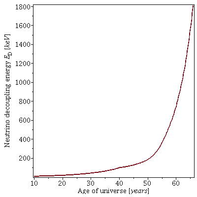
Figure 1: The energy threshold $E_{\rm D}$ of decoupling neutrinos versus age.

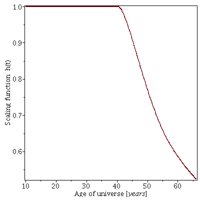
Figure 2: The scaling function h(t) for neutrino densities.

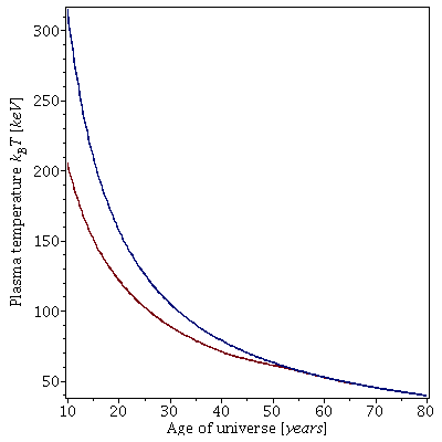
Figure 3: Plasma temperature versus age. Plasma temperature versus age for a pure photon plasma is included for comparison (top curve).

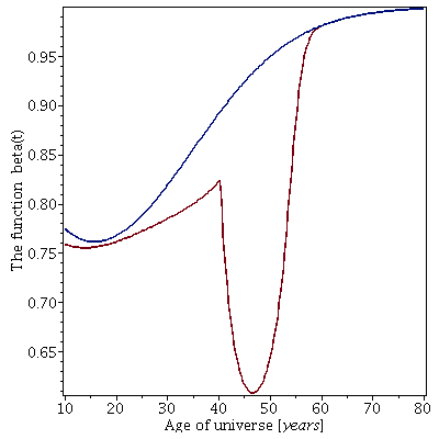
Figure 4: The function ${\beta}(t)$. The function ${\beta}(t)$ without the contribution from neutrinos is included for comparison (top curve).

Also, in this case the neutrino distributions should be significantly depleted for energies above about $3k_{\rm B}T_{\rm dec}$.

We could also try to estimate the temperature and age at neutrino decoupling for a “coasting power-law” cosmology (CPLC), i.e., a Robertson-Walker model where the Friedmann equations are made irrelevant by postulating a scale factor $a(t){\propto}t^{\alpha}$ with ${\alpha}=1$. See, e.g., [8] for more details on such a cosmology. For a general power-law cosmology with arbitrary $\alpha$, standard thermodynamics applies, so entropy conservation for the total entropy yields $s(t)t^{3{\alpha}}={\rm constant}$. Assuming that the neutrinos share most of the heating coming from net electron-positron annihilation so that the neutrinos and the photon plasma have approximately the same temperature, equation (32) yields (assuming massless neutrinos and ${\mu}_{{\nu}_{i}}{\equiv}0$)

$$T{\approx}{\frac{t_{0}^{\alpha}T_{0}}{t^{\alpha}}}{\Big{(}}{\frac{{\frac{4}{3}}{\varepsilon}_{\gamma}+\sum_{i}{\Big{[}}2{\varepsilon}_{{\nu}_{i}}^{\rm dec}(t_{0})+2p_{{\nu}_{i}}^{\rm dec}(t_{0}){\Big{]}}{\frac{T^{4}}{T_{0}^{4}}}}{{\frac{4}{3}}{\varepsilon}_{\gamma}+\sum_{i}{\Big{[}}{\varepsilon}_{{\rm p}_{i}}+{\varepsilon}_{{\rm{\bar{p}}}_{i}}+p_{{\rm p}_{i}}+p_{{\rm{\bar{p}}}_{i}}-{\mu}_{i}(n_{{\rm p}_{i}}-n_{{\rm{\bar{p}}}_{i}})+2{\varepsilon}_{{\nu}_{i}}+2p_{{\nu}_{i}}{\Big{]}}}}{\Big{)}}^{\frac{1}{3}},$$ (59)

where $2\sum_{i}{\varepsilon}_{{\nu}_{i}}^{\rm dec}(t_{0})$ is the energy density of the relic neutrino/antineutrino background at the present era. However, since the approach used in this paper is inconsistent with standard thermodynamics, equation (57) (with ${\alpha}=1)$ is not consistent with equation (27). This means that it is not meaningful to apply the model given by equation (37) to CPLCs. To estimate the decoupling temperature $T_{\rm dec}$ and decoupling era $t_{\rm dec}$ for a CPLC, we may rather try the usual approach assuming instantaneous decoupling. The decoupling criterion ${\Gamma}^{\rm eff}_{\rm scat}T/{\mid}{\dot{T}}{\mid}{\sim}1$ then yields (using equations (44) and (57)) $T_{\rm dec}{\approx}64$ keV$/k_{\rm B}$ and $t_{\rm dec}{\approx}52$ years. This result is not very different from that obtained for the quasi-metric model. Finally, we note that the decoupling temperature for a coasting cosmology was estimated to be about $75$ keV$/k_{\rm B}$ (using $H(t_{0})=65{\ }{\frac{{\rm km}}{{\rm sMpc}}}$) in [8], using a criterion ${\Gamma}_{\rm weak}/H{\sim}1$ without thermal averaging and assuming that this quantity approximately goes as ${\Big{[}}{\frac{T}{1.6{\times}10^{8}{\ }{\rm K}}}{\Big{]}}^{4}{\exp}(-m_{e}c^{2}/k_{\rm B}T)$ for the relevant temperature range.

4.4 The neutrino distributions after decoupling

In the previous section we found that the process of neutrino decoupling is estimated to take several years. It is expected that such a gradual neutrino decoupling will result in nonthermal neutrino number and energy densities of the decoupled neutrinos. Since the cosmic expansion does not redshift momenta of free neutrinos (if no mass eigenstate is null), the neutrino number and energy density distributions just after decoupling directly yield the predicted relic neutrino distributions today since the decoupled densities evolve as $t^{-3}$ once all neutrinos have decoupled.

To begin with it is straightforward to estimate the number density $n_{\nu}^{\rm dec}(t)$ as a function of time by integrating equation (39) numerically. (See appendix A for details how to do this.) The result is plotted in fig. 5. In particular we find $n_{\nu}^{\rm dec}(t_{\rm dec}){\approx}1.5{\times}10^{27}$ cm^-3. One may also estimate the number density of neutrinos decopled via interactions only by omitting the last term of equation (39). The result found is that at epoch $t_{\rm C}$, about 44${\%}$ of all neutrinos have decoupled via interactions, while at epoch $t_{\rm dec}$, this number has diminished to about 17${\%}$. Thus the low-energy part of the decoupled neutrinos has a significant number of neutrinos which decoupled via interaction, while the high-energy part consists almost only of neutrinos that have “frozen in”. This indicates that the approximate model given by equations (37) and (46) overestimates thermal contact via elastic neutrino scattering for the later stages of neutrino decoupling such that the estimated value of $T_{\rm dec}$ may be too low. The existence of approximately thermal high-energy tails of the decoupled neutrino distributions is also thrown further in doubt.

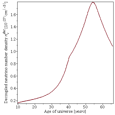
Figure 5: Decoupled neutrino number density $n^{\rm dec}_{\nu}$ versus age.

Moreover one may estimate the energy density ${\varepsilon}_{\nu}^{\rm dec}(t)$ as a function of time by integrating equation (42) numerically. But it is more interesting to estimate the average neutrino energy per particle for the decoupled neutrinos, i.e., ${\langle}E^{\rm dec}_{\nu}{\rangle}={\frac{{\varepsilon}_{\nu}^{\rm dec}}{n^{\rm dec}_{\nu}}}$. The result is plotted as a function of time in fig. 6. After all neutrinos have decoupled, they have an average energy of about 168 keV. On the other hand there is not enough information to calculate the number density distribution $n^{\rm dec}_{\nu}(E_{\nu}^{\rm dec})$ or the energy density distribution ${\varepsilon}^{\rm dec}_{\nu}(E_{\nu}^{\rm dec})$.

Once the neutrinos have decoupled, they will stream freely outwards from the last scattering surface with a speed close to the speed of light. Just after the last scattering the neutrinos are in their flavour eigenstates. However, the flavour eigenstates may be described as wave-packets consisting of a superposition of mass eigenstates with different masses. The different mass eigenstates ${\nu}_{j}$ (with mass $m_{j}$) will propagate with different speeds $v_{j}$, leading to wave-packet separation and decoherence. This means that, soon after decoupling, the decoupled neutrinos will propagate as separate mass eigenstates and not as flavour eigenstates.

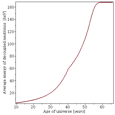
Figure 6: Average energy of decoupled neutrinos ${\langle}E^{\rm dec}_{\nu}{\rangle}$ versus age.

4.5 The predicted relic neutrino background

The main result of the previous section was the prediction from quasi-metric cosmology that the cosmological neutrino background just after decoupling would be nonthermal. Moreover, if we assume the approximate validity of equation (37) throughout neutrino decoupling, the negligible decoupling via interaction towards the end indicates the existence of a “frozen in” high-energy tail of the neutrino energy distribution. This high-energy tail should be approximately thermal, so that the non-thermal features apply mainly to the low-energy part of the neutrino energy distribution. Furthermore, over time this neutrino background will keep its (nonthermal) characteristic with all neutrinos having the same energy they had just after decoupling, yielding a “high-energy” relic neutrino background today. In addition, today’s relic neutrino background should be in the form of separate neutrino mass eigenstates since the heavier mass eigenstates should trail far behind the lightest mass eigenstate.

Standard cosmology predicts a cosmic neutrino number density of each flavour (neutrinos plus antineutrinos) of about $112$ cm^-3 and a neutrino relic background very close to thermal with an “effective” temperature [9] of about $1.96$ K. Moreover, data from neutrino oscillation experiments yield information on the quantities ${\Delta}m_{ij}^{2}{\equiv}{\mid}m_{i}^{2}-m_{j}^{2}{\mid}$. That is, ${\Delta}m_{21}^{2}c^{4}=7.50^{+0.18}_{-0.19}{\times}10^{-5}$ eV² and ${\Delta}m_{31}^{2}c^{4}=2.47^{+0.170}_{-0.067}{\times}10^{-3}$ eV² (see, e.g. [10]). This means, assuming a “normal” mass hierarchy, that $m_{3}c^{2}>m_{2}c^{2}{\gg}k_{\rm B}T_{\nu}{\sim}1.7{\times}10^{-4}$ eV, i.e., that at least the two most massive relic neutrino mass eigenstates will be nonrelativistic. Thus the cosmic neutrino background as predicted from standard cosmology should be nonrelativistic at the present epoch. On the other hand, quasi-metric cosmology predicts a relic neutrino backround with properties very different from its counterpart in standard cosmology, so a crucial question is if the existence of this nonstandard background would be consistent with current experimental results. To answer that, we must first find the flux of background neutrinos at the present epoch. Since after neutrino decoupling, ${\beta}(T){\approx}1$ to a good approximation, we find from the previous section that the present number density of each neutrino mass eigenstate ${\nu}_{j}$, i.e., $n_{{\nu}_{j}}(t_{0})$, is approximately equal to an effective number density of each neutrino flavour eigenstate ${\nu}_{\alpha}$ of $n_{{\nu}_{\alpha}}(t_{0})={\frac{t_{\rm dec}^{3}}{t_{0}^{3}}}n_{{\nu}_{\alpha}}(t_{\rm dec}){\approx}129$ cm^-3. That is, the effective number density of neutrinos plus antineutrinos of each flavour is about $258$ cm^-3. This is more than twice the number density predicted from standard cosmology.

The above neutrino number density predictions from quasi-metric cosmology imply that the effective flux of relic electron-neutrinos at the present era is predicted to be about $cn_{{\nu}_{e}}(t_{0}){\approx}3.9{\times}10^{12}$ cm^-2s^-1. This may be compared to the flux of low-energy electron-neutrinos produced in nuclear reactions taking place in the Sun’s core (as predicted from standard solar models) and measured at the Earth. That is, while the total flux of solar neutrinos is predicted to be about $6.5{\times}10^{10}$ cm^-2s^-1, the flux of low-energy neutrinos is predicted to be about $6.0{\times}10^{10}$ cm^-2s^-1 and to arise from the dominant proton-proton chain. These predictions of solar neutrino fluxes agree very well with measurements made in the Borexino experiment [11]. On the other hand, the effective estimated total flux of cosmic electron-neutrinos coming from quasi-metric cosmology exceeds the estimated total flux of solar neutrinos by a factor of about 60, indicating a violent conflict with this experiment. Said prediction is also inconsistent with experiments (GALLEX/GNO, SAGE) detecting low-energy neutrinos from the Sun using the reaction ${}^{71}{\rm Ga}+{\nu}_{e}{\ }{\rightarrow}{\ }^{71}{\rm Ge}+e^{-}$. (In this reaction, the neutrino is required to have a minimum energy of ${\rm E}_{\nu}^{\rm min}=233$ keV.) In particular, the experiment SAGE measured an electron-neutrino capture rate consistent with an electron-neutrino flux at the location of the Earth of about $3.4{\times}10^{10}$ cm^-2s^-1 coming from the proton-proton chain [12]. (The discrepancy with said theoretical result of about $6.0{\times}10^{10}$ cm^-2s^-1 is explained as an effect due to neutrino oscillations.) On the other hand, we may estimate an “effective” cosmic electron-neutrino flux assuming that relic neutrinos with energy above said minimum energy are given approximately by equation (37) with $E_{\rm D}{\approx}E^{\rm min}_{\nu}$ corresponding to an age $t_{\rm min}{\approx}52$ yr and a plasma temperature $T_{\rm min}{\approx}59$ keV/$k_{\rm B}$, i.e.,

$${\Phi}_{{\nu}_{e}}^{\rm cosm}(E_{\nu}{\geq}{E_{\nu}^{\rm min}}){\approx}{\frac{t_{\rm min}^{3}}{t_{0}^{3}}}{\frac{h(t_{\rm min})k_{\rm B}^{3}T_{\rm min}^{3}}{2{\pi}^{2}{\hbar}^{3}c^{2}}}{\int}_{{\!}{\!}{\!}{\!}{\frac{E_{\nu}^{\rm min}}{k_{\rm B}T_{\rm min}}}}^{\infty}{\frac{x^{2}dx}{1+e^{x}}}{\approx}8.7{\times}10^{11}{\ }{\rm cm}^{-2}{\rm s}^{-1},$$ (60)

demonstrating that the effective flux of cosmic electron neutrinos in the relevant energy range is about 13 times the total flux of solar neutrinos. This means that the possible existence of the predicted relic cosmic neutrino background is strongly inconsistent with experimental data. This conclusion is confirmed by calculating the corresponding capture rate $R^{\rm cosm}_{{\nu}_{e}}$ of cosmological electron-neutrinos in a ${}^{71}{\rm Ga}$-detector. This is given by (using a similar definition as given in [12] for $240{\ }{\rm keV}{\leq}E_{\nu}{\leq}733{\ }{\rm keV}$)

$$R_{{\nu}_{e}}^{\rm cosm}{\equiv}{\int}_{{\!}{\!}{240{\ }{\rm keV}}}^{733{\ }{\rm keV}}{\sigma}_{\rm Ga}(E_{\nu}){\Upsilon}^{\rm cosm}_{{\nu}_{e}}(E_{\nu})dE_{\nu},\quad{\Upsilon}^{\rm cosm}_{{\nu}_{e}}(E_{\nu}){\equiv}{\frac{t_{\rm min}^{3}}{t_{0}^{3}}}{\frac{h(t_{\rm min})}{2{\pi}^{2}{\hbar}^{3}c^{2}}}{\frac{E_{\nu}^{2}}{[1+{\exp}(E_{\nu}/k_{\rm B}T_{\rm min})]}},$$

$${\sigma}_{\rm Ga}(E_{\nu}){\approx}[13.10+91.29({\frac{E_{\nu}}{1{\ }{\rm MeV}}}-0.24{\ })^{1.157}]{\times}10^{-46}{\ }{\rm cm}^{2},$$ (61)

where ${\sigma}_{\rm Ga}(E_{\nu})$ is the estimated cross section for neutrino capture by ${}^{71}{\rm Ga}$ given in [12] (we have used the fact that contributions to $R_{{\nu}_{e}}^{\rm cosm}$ are negligibile for $E_{\nu}>733$ keV). Moreover, ${\Upsilon}^{\rm cosm}(E_{\nu})$ is the estimated differential flux of cosmic neutrinos with energy $E_{\nu}$. By inserting the expression for ${\sigma}_{\rm Ga}(E_{\nu})$ into equation (59) we find a rate of $R^{\rm cosm}_{{\nu}_{e}}{\sim}15{\times}10^{-34}$ s${}^{-1}{\equiv}1.5{\times}10^{3}$ SNU. However, the weighted combination of all observational Ga-experiments yields a result of only about $66$ SNU [12], to be compared to the calculated contribution from solar neutrinos given by 128 SNU (without taking into account neutrino oscillations). In other words, the existence of a cosmic neutrino backround with an approximately thermal high-energy tail with temperature of about $50-60$ keV/$k_{\rm B}$ is in violent conflict with gallium experiments as well.

However, as mentioned above, one might argue that any thermal high-energy tail is expected to be significantly depleted due to severe deviations from equilibrium towards the end of neutrino decoupling. This could make it possible in principle (but not very likely), to reduce the density of relic neutrinos with energy above 233 keV with the necessary factor of about 1000 or more. On the other hand, in the Borexino experiment one has deteced solar neutrinos with energies down to 165 keV without finding any excess other than the expected effects coming from radiative decay of ¹⁴C naturally occuring in the organic detector fluid [11]. For such low energies excess detections due to relic neutrinos are expected to be seen anyway, meaning that said conflict can be resolved only by invoking non-standard neutrino physics. In particular, if neutrinos are unstable, decaying into massless or “invisible” particles, neutrino decay is a possible way out.

5 Remarks on primordial nucleosynthesis

As shown in the previous section, barring neutrino decay the kinematics of massive neutrinos after decoupling implies that the cosmic neutrino background as predicted from the QMF is in violent conflict with observations. Nevertheless, it may be of interest using the QMF to calculate the abundances of light nuclei synthesized in the early Universe and see if such calculations are consistent with observations. However, full quantitative nucleosynthesis calculations are beyond the scope of this paper, but some estimates and qualitative arguments based on the results of the previous section shall be made. Fortunately said calculations have already been done for power-law cosmologies [8,13,14], and in particular for CPLCs [14, 15]. Qualitative comparisons with the main results found from these calculations is the subject of this section.

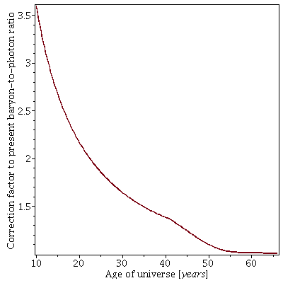
Figure 7: Correction factor to today’s value of $n_{b}/n_{\gamma}$ versus age.

There are two main differences between primordial nucleosynthesis in the QMF as compared to power-law cosmologies. First, the temperature evolution for the power-law cosmologies is given from equation (57) for different values of ${\alpha}$. This differs substantially from the temperature evolution given from equations (27) and (43). In particular, for CPLCs, the temperature evolution goes approximately as $1/t$, whereas for the quasi-metric cosmology we see from fig. 3 that the temperature drops (much) slower than $1/t$ during (and before) the era of electron-positron annihilation. This means that the quasi-metric universe at the same temperature is younger (and denser) than for the CPLCs during the main nucleosynthesis era. Second, the baryon to photon ratio $n_{b}/n_{\gamma}$ is not a constant in quasi-metric cosmology since it decreases whenever ${\beta}(T)<1$. This means that for much of the epoch of primordial nucleosynthesis, the value of $n_{b}/n_{\gamma}$ was higher than it is today (see fig. 7). On the other hand, for the power-law cosmologies (and for standard cosmology), said value is constant from the epoch of primordial nucleosynthesis until today.

To get primordial nucleosynthesis started, there must be a supply of neutrons. For a CPLC as for quasi-metric cosmology, the universe is so old at the relevant temperatures that the only way to have a supply of neutrons is to produce them is via the weak-interaction reactions [15]

$$n{\rightleftharpoons}p+e^{-}+{\bar{\nu}}_{e},\qquad n+e^{+}{\rightleftharpoons}p+{\bar{\nu}}_{e},\qquad p+e^{-}{\rightleftharpoons}n+{\nu}_{e}.$$ (62)

Due to slowly changing plasma temperatures, these reactions will remain in equilibrium almost down to temperatures where significant neutrino decoupling occurs. See [16] for explict expressions for the reaction rates (per nucleon) ${\lambda}_{{\rm n}{\rightarrow}{\rm p}}$ and ${\lambda}_{{\rm p}{\rightarrow}{\rm n}}$ for the reactions shown in equation (60). (Note that in general, $T_{\nu}{\neq}T_{\gamma}$ in said expressions.) Now the period where the ⁴He is synthesized is limited to the period before the reactions $p{\rightarrow}n$ shown in equation (60) freeze out, since after freeze-out, the neutron-to-proton ratio will no longer depend on temperature and subsequently the free neutrons will decay quickly leaving almost no neutrons left available for additional nucleosynthesis. Said limitation of the ⁴He-synthesis period is valid both for the CPLCs and for the quasi-metric universe, but as mentioned above the quasi-metric universe is younger and denser at the same temperatures but yet such that the temperatures drop more slowly. Also $n_{b}/n_{\gamma}$ is higher at early epochs than today. All this means that there is more time available for ⁴He-production at the relevant temperatures than in the CPLCs, so it might be possible to produce a sufficient amount of ⁴He without needing a very high ratio $n_{b}/n_{\gamma}$ today. On the other hand, to get the right amount of ⁴He for a CPLC (assuming that ${\mu}_{{\nu}_{i}}=0$), one must have $n_{b}/n_{\gamma}{\approx}1.05{\times}10^{-8}$ today [15], i.e., much larger than the value of $(6.10{\pm}0.04){\times}10^{-10}$ [17] as inferred by analysing the cosmic microwave background assuming standard cosmology. It is possible for a CPLC to produce a sufficient amount of ⁴He with a significantly smaller value of $n_{b}/n_{\gamma}$ by assuming a suitable neutrino asymmetry (i.e., ${\mu}_{{\nu}_{i}}<0$) [15].

Another serious problem for both the CPLCs and for quasi-metric cosmology is the severe primordial underproduction of the light elements D, ³He and ⁷Li. Deuterium is produced/destroyed via the reactions

$$n+p{\rightleftharpoons}{\rm D}+{\gamma},\quad p+p{\rightarrow}{\rm D}+e^{+}+{\nu}_{e},\quad{\rm D}+p{\rightleftharpoons}^{3}{\rm He}+{\gamma},\quad^{3}{\rm He}+{\rm D}{\rightarrow}^{4}{\rm He}+p.$$ (63)

However, at the relevant temperatures of ⁴He-synthesis, due to the weakly bound D-nucleus and the long time available for nucleosynthesis, almost any produced D has been destroyed when the reactions shown in equation (61) eventually freeze out. The same comment applies to most produced ³He via the third reaction shown in equation (61), since it will be destroyed via the reaction ${}^{3}{\rm He}+p{\rightarrow}^{4}{\rm He}+e^{+}+{\nu}_{e}$. Similarly, almost any produced ⁷Li will be destroyd via the reaction ${}^{7}{\rm Li}+p{\rightarrow}^{4}{\rm He}+^{4}{\rm He}$. See, e.g., [14, 15] for detailed abundances calculated as functions of temperature for CPLCs. To get acceptable levels of D, ³He and ⁷Li, these nuclei must be produced much later in the history of the universe, in environments where destruction rates of said nuclei are not crucial. For the CPLCs, spallation processes connected to protostar formation have been proposed as a mechanism for producing the missing light elements [15].

Quasi-metric cosmology shares the problem of said missing light elements with the CPLCs. However, since the primordial abundance of D is inferred from analysing absorption line systems in spectra of quasi-stellar objects (QSOs) (D/H$=(2.53{\pm}0.10){\times}10^{-5}$ by number [18]), the nature of QSOs may be crucial when interpreting these results. That is, the interpretation of QSOs and their absorption line systems within quasi-metric cosmology may be very different from the standard one and such that there is a possibility that the missing light elements may be produced within the QSOs themselves (possibly via spallation mechanisms). Moreover, there are in fact no direct observational data on primordial abundances of ³He; data for abundances of ³He (³He/H$=(1.01{\pm}0.2){\times}10^{-5}$ by number [19]) are limited to within our galaxy and represent upper limits to the primordial abundance.

6 Conclusion

The main result of this paper is that assuming the validity of standard neutrino physics and the approximate model given by equation (37), the calculated properties of the predicted cosmic relic neutrino background as obtained from the QMF are in gross conflict with observations. This means that, with no natural explanation to resolve said conflict, the QMF is currently nonviable. The nonviable status of the QMF can only be revoked by experimental evidence indicating new, exotic neutrino physics. One theoretical possibility of such is if the lightest mass eigenstate ${\nu}_{1}$ (normal hierarchy) is null (and thus stable) and the other two massive eigenstates decay into ${\nu}_{1}$ and some other (possibly massless) particle $X$, i.e.,

$${\nu}_{i}{\rightarrow}{\nu}_{1}+X,\qquad i{\in}{\{}2,3{\}}.$$ (64)

Since there are strong restrictions on neutrino radiative decay from observations of solar neutrinos and neutrinos observed from supernova 1987A (see, e.g., [20]), $X$ can hardly be a photon. That is, said restrictions yield ${\tau}_{{\nu}_{i},0}/m_{{\nu}_{i}}c^{2}{\gtrsim}10^{15}$ s/eV, where ${\tau}_{{\nu}_{i},0}$ is the lifetime of mass eigenstate ${\nu}_{i}$ in its rest frame. However, the reduction in relic neutrino numbers with a factor 1000 or more needed to avoid said conflict with experiment yields ${\tau}_{{\nu}_{i},0}/m_{{\nu}_{i}}c^{2}{\lesssim}10^{11}$ s/eV (by solving the decay equation). On the other hand, neutrino non-radiative decay is much less restricted by observations. That is, $X$ might be a light (possibly massless) sterile mass eigenstate ${\nu}_{{\rm s}}$ (that may or may not be accessible via neutrino oscillations) [21]. We note that there exists a number of estimates of neutrino decay limits and lifetimes (see, e.g., [22] for a review), but most are model-dependent and not stringent enough to rule out a potential resolution of said conflict.

If future experiments show that no neutrino mass eigenstate is null, the only possibility left would be decay of all neutrino mass eigenstates into “invisible” particles over cosmic time scales; this seems rather farfetched and difficult to test. Nevertheless this possibility cannot be dismissed out of hand. However, as long as there is no independent experimental evidence that neutrinos really do decay, the QMF should be declared nonviable.
Acknowledgement
I wish to thank Dr. Kåre Olaussen for reviewing the manuscript.
References
[1] D. Østvang, Grav. & Cosmol. 11, 205 (2005) (gr-qc/0112025).
[2] D. Østvang, Doctoral thesis, (2001) (gr-qc/0111110).
[3] D. Østvang, Grav. & Cosmol. 13, 1 (2007) (gr-qc/0201097).
[4] V. Mukhanov, Physical Foundations of Cosmology,
       Cambridge University Press, 2005.
[5] E.W. Kolb and M.S. Turner, The Early Universe, Addison-Wesley, 1990.
[6] C. Giunti and C.W. Kim, Fundamentals of Neutrino Physics and Astrophysics,
      Oxford University Press, 2007.
[7] D.A. Dicus, Phys. Rev. D 6, 941 (1972).
[8] A. Batra, D. Lohiya, S. Mahajan and A. Mukherjee, IJMP D 9, 757 (2000)
      (nucl-th/9902022).
[9] H. Zhang, Class. Quantum Grav. 25, 208001 (2008) (arXiv:0808.1552)
[10] M.C. Gonzalez-Garcia, M. Maltoni, J. Salvado and T. Schwetz, JHEP 12, 123 (2012)
       (arXiv:1209.3023).
[11] G. Bellini et al., Nature 512, 383 (2014).
[12] J.N. Abdurashitov et al., Phys. Rev. C 80, 015807 (2009) (arXiv:0901.2200).
[13] M. Sethi, A. Batra and D. Lohiya, Phys. Rev. D 60, 108301 (1999)
       (astro-ph/9903084).
[14] M. Kaplinghat, G. Steigman and T. P. Walker, Phys. Rev. D 61, 103507 (2000)
       (astro-ph/9911066).
[15] P. Singh and D. Lohiya, JCAP 05, 061 (2015) (arXiv:1312.7706).
[16] G. Beaudet and P. Goret, Astron. Astrophys. 49, 415 (1976).
[17] P.A.R. Ade et al., A&A 594, A13 (2016) (arXiv:1502.01589).
[18] R. Cooke et al., ApJ 781, 31 (2014).
[19] T.M. Bania, R.T. Rood and D. S. Balser, Nature 415, 54 (2002).
[20] E.L. Chupp, W.T. Vestrand and C. Reppin, Phys. Rev. Lett. 62, 505 (1989).
[21] J.F. Beacom and N.F. Bell, Phys. Rev. D 65, 113009 (2002) (hep-ph/0204111).
[22] K. A. Olive et al., Chin. Phys. C 38, 090001 (2014).
[23] F. Debbasch and W.A. van Leeuwen, Physica A 388, 1818 (2009).

Appendix A Integrodifferential equations

In this appendix we give explicit expressions for the integrodifferential equations (27) for $T(t)$ and (40) for $h(t)$, using equation (43) for ${\beta}(T)$. In addition we have the thermally non-averaged decoupling criterion (45) for $E_{\rm D}$. Setting $w{\equiv}E_{\rm D}/m_{e}c^{2}$, $y{\equiv}m_{e}c^{2}/k_{\rm B}T$, equation (27) reads

$$t{\frac{dy}{dt}}-{\beta}(y,w,h,t)y=0,$$ (A.1)

where ${\beta}(y,w,h,t)$ is found from equation (43), i.e.,

$${\beta}(y,w,h,t){\approx}{\frac{1+{\frac{45y^{4}}{2{\pi}^{4}}}{\int}_{{\!}{\!}1}^{\infty}{\frac{x^{2}{\sqrt{x^{2}-1}}dx}{1+{\exp}(yx)}}}{1+{\frac{30y^{4}}{{\pi}^{4}}}{\int}_{{\!}{\!}1}^{\infty}{\frac{x^{2}{\sqrt{x^{2}-1}}dx}{1+{\exp}(yx)}}+{\frac{15y^{4}}{2{\pi}^{4}}}{\int}_{{\!}{\!}1}^{\infty}{\frac{x^{2}dx}{{\sqrt{x^{2}-1}}[1+{\exp}(yx)]}}+{\frac{45h}{4{\pi}^{4}}}{\int}_{{\!}{\!}yw}^{\infty}{\frac{x^{3}dx}{1+{\exp}(x)}}}}$$

$$+{\frac{{\frac{45h}{4{\pi}^{4}}}{\int}_{{\!}{\!}yw}^{\infty}{\frac{x^{3}dx}{1+{\exp}(x)}}[{\Gamma}^{\rm net}_{\rm ann}-{\frac{2}{3{\zeta}(3)}}{\int}_{{\!}{\!}0}^{yw}{\frac{x^{2}dx}{1+{\exp}(x)}}{\Gamma}_{\rm scat}^{\rm eff}]t+{\frac{15h}{2{\pi}^{4}{\zeta}(3)}}{\int}_{{\!}{\!}0}^{yw}{\frac{x^{3}dx}{1+{\exp}(x)}}{\int}_{{\!}{\!}yw}^{\infty}{\frac{x^{2}dx}{1+{\exp}(x)}}{\Gamma}_{\rm scat}^{\rm eff}t}{1+{\frac{30y^{4}}{{\pi}^{4}}}{\int}_{{\!}{\!}1}^{\infty}{\frac{x^{2}{\sqrt{x^{2}-1}}dx}{1+{\exp}(yx)}}+{\frac{15y^{4}}{2{\pi}^{4}}}{\int}_{{\!}{\!}1}^{\infty}{\frac{x^{2}dx}{{\sqrt{x^{2}-1}}[1+{\exp}(yx)]}}+{\frac{45h}{4{\pi}^{4}}}{\int}_{{\!}{\!}yw}^{\infty}{\frac{x^{3}dx}{1+{\exp}(x)}}}}.$$ (A.2)

Here, we have from equations (44) and (55) that

$${\Gamma}_{\rm scat}^{\rm eff}={\frac{3}{2}}{\zeta}(3)K{\frac{I(y)}{{\frac{3}{2}}{\zeta}(3)-J(yw)}}{\Big{\{}}{\frac{b}{y}}{\Big{[}}I_{1}(y,w)-I_{3}(y,w)+{\frac{2}{3}}I_{4}(y,w){\Big{]}}-aI_{2}(y,w){\Big{\}}},$$ (A.3)

where we have defined $a{\equiv}2{\sin}^{2}{\theta}_{\rm w}(6{\sin}^{2}{\theta}_{\rm w}-1){\approx}0.1748$, $b{\equiv}24{\sin}^{4}{\theta}_{\rm w}-4{\sin}^{2}{\theta}_{\rm w}+3{\approx}3.3496$ and $K{\equiv}{\frac{4G_{\rm F}^{2}m_{e}^{5}c^{4}}{9{\pi}^{3}{\zeta}(3){\hbar}^{7}}}{\approx}8.5855{\times}10^{-5}$ s${}^{-1}{\approx}2.7075{\times}10^{3}$ yr^-1. Also, $I_{1}(y,w)$, $I_{2}(y,w)$, $I_{3}(y,w)$ and $I_{4}(y,w)$ are given from equation (52) and we have defined

$$I(y){\equiv}{\int}_{{\!}{\!}{\!}{\!}1}^{\infty}{\frac{x{\sqrt{x^{2}-1}}dx}{1+{\exp}(yx)}},$$ (A.4)

in addition to

$$J(u){\equiv}{\int}_{{\!}{\!}{\!}{\!}0}^{u}{\frac{x^{2}dx}{1+e^{x}}}={\frac{3}{2}}{\zeta}(3)+{\frac{1}{3}}u^{3}-u^{2}{\ln}(1+e^{u})-2u{\rm Li}_{2}(-e^{u})+2{\rm Li}_{3}(-e^{u}),$$ (A.5)

where ${\rm Li}_{s}(z)$ is the polylogarithm, defined by

$${\rm Li}_{s}(z){\equiv}\sum_{k=1}^{\infty}{\frac{z^{k}}{k^{s}}},\qquad z{\in}{\bf C}.$$ (A.6)

We notice the exact expression

$${\int}_{{\!}{\!}{\!}{\!}u}^{\infty}{\frac{x^{3}dx}{1+e^{x}}}={\frac{7{\pi}^{4}}{60}}-{\frac{1}{4}}u^{4}+u^{3}{\ln}(1+e^{u})+3u^{2}{\rm Li}_{2}(-e^{u})-6u{\rm Li}_{3}(-e^{u})+6{\rm Li}_{4}(-e^{u}).$$ (A.7)

Next, for epochs $t{\leq}t_{\rm C}$, we have from equation (40) that

$${\Gamma}^{\rm net}_{\rm ann}{\approx}{\frac{3}{t}}{\Big{(}}1-{\beta}(y,w,t){\Big{)}}+{\frac{2}{3{\zeta}(3)}}\int_{0}^{yw}{\frac{x^{2}dx}{{\exp}(x)+1}}{\Gamma}^{\rm eff}_{\rm scat},\qquad t{\leq}t_{\rm C},$$ (A.8)

since $h=1$ and ${\dot{h}}=0$ for this time interval. For later times $t{\geq}t_{\rm C}$, ${\Gamma}^{\rm net}_{\rm ann}$ will be smaller and its decline is determined by the evolution of the thermally averaged annihilation rate (producing neutrinos). The latter can be found from the number density of electrons/positrons and the size of the thermally averaged cross sections shown in equation (56). Therefore, with ${\beta}_{\rm C}{\equiv}{\beta}(y_{\rm C},w_{\rm C},t_{\rm C})$, $I_{1{\rm C}}{\equiv}I_{1}(y_{\rm C},w_{\rm C})$ etc., we can set (see also equation (A.18) below)

$${\Gamma}^{\rm net}_{\rm ann}{\approx}{\Big{[}}{\frac{3}{t_{\rm C}}}(1-{\beta}_{\rm C})+{\frac{2}{3{\zeta}(3)}}J(y_{\rm C}w_{\rm C}){\Gamma}^{\rm eff}_{\rm scat}(y_{\rm C},w_{\rm C}){\Big{]}}$$

$${\times}{\frac{I(y){\Big{(}}b[4I_{5}(y)-I(y)]+3a[2I(y)-{\frac{1}{2}}I_{6}(y)]{\Big{)}}}{I(y_{\rm C}){\Big{(}}b[4I_{5}(y_{\rm C})-I(y_{\rm C})]+3a[2I(y_{\rm C})-{\frac{1}{2}}I_{6}(y_{\rm C})]{\Big{)}}}}$$

$$={\Big{[}}{\frac{3}{t_{\rm C}}}(1-{\beta}_{\rm C})+{\frac{KJ({y_{\rm C}w_{\rm C}})I(y_{\rm C})}{{\frac{3}{2}}{\zeta}(3)-J({y_{\rm C}w_{\rm C}})}}{\Big{\{}}{\frac{b}{y_{\rm C}}}{\Big{(}}I_{1{\rm C}}-I_{3{\rm C}}+{\frac{2}{3}}I_{4{\rm C}}{\Big{)}}-aI_{2{\rm C}}{\Big{\}}}{\Big{]}}$$

$${\times}{\frac{I(y){\Big{(}}b[4I_{5}(y)-I(y)]+3a[2I(y)-{\frac{1}{2}}I_{6}(y)]{\Big{)}}}{I(y_{\rm C}){\Big{(}}b[4I_{5}(y_{\rm C})-I(y_{\rm C})]+3a[2I(y_{\rm C})-{\frac{1}{2}}I_{6}(y_{\rm C})]{\Big{)}}}},\qquad t{\geq}t_{\rm C},$$ (A.9)

where $I_{5}(y)$ and $I_{6}(y)$ are defined in equation (54). Now, combining equations (40) and (A.9) we find the equation

$${\frac{1}{h}}{\frac{dh}{dt}}+{\frac{3}{t}}(1-{\beta})+{\frac{KJ(yw)I(y)}{{\frac{3}{2}}{\zeta}(3)-J(yw)}}{\Big{\{}}{\frac{b}{y}}{\Big{[}}I_{1}-I_{3}+{\frac{2}{3}}I_{4}{\Big{]}}-aI_{2}{\Big{\}}}$$

$$-{\Big{[}}{\frac{3}{t_{\rm C}}}(1-{\beta}_{\rm C})+{\frac{KJ(y_{\rm C}w_{\rm C})I(y_{\rm C})}{{\frac{3}{2}}{\zeta}(3)-J(y_{\rm C}w_{\rm C})}}{\Big{\{}}{\frac{b}{y_{\rm C}}}{\Big{[}}I_{1{\rm C}}-I_{3{\rm C}}+{\frac{2}{3}}I_{4{\rm C}}{\Big{]}}-aI_{2{\rm C}}{\Big{\}}}{\Big{]}}$$

$${\times}{\frac{I(y){\Big{(}}b[4I_{5}(y)-I(y)]+3a[2I(y)-{\frac{1}{2}}I_{6}(y)]{\Big{)}}}{I(y_{\rm C}){\Big{(}}b[4I_{5}(y_{\rm C})-I(y_{\rm C})]+3a[2I(y_{\rm C})-{\frac{1}{2}}I_{6}(y_{\rm C})]{\Big{)}}}}=0,\qquad t{\geq}t_{\rm C},$$ (A.10)

valid for $t{\geq}t_{\rm C}$. The third equation needed to close the set of equations is obtained from the criterion (46), written in the form

$$G_{\rm scat}(y,w,h,t)={\frac{3}{2}}{\zeta}(3)K{\frac{tI(y)}{{\beta}(y,w,h,t)}}{\frac{w^{2}}{1+2w}}{\Big{[}}b-{\frac{a+bw}{1+2w}}+{\frac{2bw^{2}}{3(1+2w)^{2}}}{\Big{]}}{\approx}1.$$ (A.11)

However, in practice it may be easier to solve numerically a third integrodifferential equation rather than the implicit relationship (A.11). In particular, trying to solve the coupled set of equations (A.1), (A.10) and (A.11) using MAPLE does not work since equation (A.11) is not separable in the variable $w$. This problem can be circumvented by taking the derivative of (A.11) with respect to $t$. We then get the equation

$${\frac{3}{2}}{\zeta}(3)K{\frac{w^{2}}{1+2w}}{\Big{[}}b-{\frac{a+bw}{1+2w}}+{\frac{2bw^{2}}{3(1+2w)^{2}}}{\Big{]}}{\Big{\{}}I(y)-{\int}_{{\!}{\!}{\!}{\!}1}^{\infty}{\frac{e^{yx}x^{2}{\sqrt{x^{2}-1}}dx}{[1+{\exp}(yx)]^{2}}}{\beta}y{\Big{\}}}$$

$$+{\frac{1}{2}}{\zeta}(3)KI(y){\frac{w}{(1+2w)^{4}}}[16bw^{3}+32bw^{2}-(12a-21b)w-6(a-b)]{\frac{tdw}{dt}}{\approx}{\frac{d{\beta}}{dt}},$$ (A.12)

where the right hand side can be found from equation (A.2), i.e.,

$${\Big{\{}}1+{\frac{30y^{4}}{{\pi}^{4}}}{\int}_{{\!}{\!}{\!}{\!}1}^{\infty}{\frac{x^{2}{\sqrt{x^{2}-1}}dx}{1+e^{yx}}}+{\frac{15y^{4}}{2{\pi}^{4}}}{\int}_{{\!}{\!}{\!}{\!}1}^{\infty}{\frac{x^{2}dx}{{\sqrt{x^{2}-1}}[1+e^{yx}]}}+{\frac{45h}{4{\pi}^{4}}}{\int}_{{\!}{\!}{\!}{\!}yw}^{\infty}{\frac{x^{3}dx}{1+e^{x}}}{\Big{\}}}{\frac{d{\beta}}{dt}}$$

$$={\Big{[}}{\frac{90y^{3}}{{\pi}^{4}}}{\int}_{{\!}{\!}{\!}{\!}1}^{\infty}{\frac{x^{2}{\sqrt{x^{2}-1}}dx}{1+{\exp}(yx)}}-{\frac{45y^{4}}{2{\pi}^{4}}}{\int}_{{\!}{\!}{\!}{\!}1}^{\infty}{\frac{e^{yx}x^{3}{\sqrt{x^{2}-1}}dx}{[1+{\exp}(yx)]^{2}}}-{\frac{45h}{4{\pi}^{4}}}{\frac{y^{3}w^{4}}{1+{\exp}(yw)}}$$

$${\times}{\Big{(}}{\Gamma}^{\rm net}_{\rm ann}-{\Gamma}^{\rm eff}_{\rm scat}{\Big{)}}t+{\beta}{\Big{\{}}-{\frac{120y^{3}}{{\pi}^{4}}}{\int}_{{\!}{\!}{\!}{\!}1}^{\infty}{\frac{x^{2}{\sqrt{x^{2}-1}}dx}{1+e^{yx}}}+{\frac{30y^{4}}{{\pi}^{4}}}{\int}_{{\!}{\!}{\!}{\!}1}^{\infty}{\frac{e^{yx}x^{3}{\sqrt{x^{2}-1}}dx}{[1+e^{yx}]^{2}}}$$

$$-{\frac{30y^{3}}{{\pi}^{4}}}{\int}_{{\!}{\!}{\!}{\!}1}^{\infty}{\frac{x^{2}dx}{{\sqrt{x^{2}-1}}[1+e^{yx}]}}+{\frac{15y^{4}}{2{\pi}^{4}}}{\int}_{{\!}{\!}{\!}{\!}1}^{\infty}{\frac{e^{yx}x^{3}dx}{{\sqrt{x^{2}-1}}[1+e^{yx}]^{2}}}+{\frac{45h}{4{\pi}^{4}}}{\frac{y^{3}w^{4}}{1+e^{yw}}}{\Big{\}}}{\Big{]}}{\frac{{\beta}y}{t}}$$

$$+{\frac{45h}{4{\pi}^{4}}}{\frac{y^{4}w^{3}}{1+e^{yw}}}{\Big{(}}{\beta}-[{\Gamma}^{\rm net}_{\rm ann}-{\Gamma}^{\rm eff}_{\rm scat}]t{\Big{)}}{\frac{dw}{dt}}-{\frac{7h}{16{\zeta}(3)}}{\frac{y^{3}w^{2}}{1+e^{yw}}}{\Gamma}^{\rm eff}_{\rm scat}{\Big{(}}{\beta}w+t{\frac{dw}{dt}}{\Big{)}}$$

$$+{\frac{45}{4{\pi}^{4}}}{\int}_{{\!}{\!}{\!}{\!}yw}^{\infty}{\frac{x^{3}dx}{1+e^{x}}}{\Big{(}}[{\Gamma}^{\rm net}_{\rm ann}-{\Gamma}^{\rm eff}_{\rm scat}]t-{\beta}{\Big{)}}{\frac{dh}{dt}}+{\frac{7}{16}}{\Big{(}}{\frac{3}{2}}-{\frac{J(yw)}{{\zeta}(3)}}{\Big{)}}{\Gamma}^{\rm eff}_{\rm scat}{\Big{(}}h+t{\frac{dh}{dt}}{\Big{)}}$$

$$+{\frac{45h}{4{\pi}^{4}}}{\int}_{{\!}{\!}{\!}{\!}yw}^{\infty}{\frac{x^{3}dx}{1+e^{x}}}{\Big{(}}{\Gamma}^{\rm net}_{\rm ann}-{\Gamma}^{\rm eff}_{\rm scat}+t{\frac{d}{dt}}{\Gamma}^{\rm net}_{\rm ann}-t{\frac{d}{dt}}{\Gamma}^{\rm eff}_{\rm scat}{\Big{)}}+{\frac{7h}{16}}{\Big{(}}{\frac{3}{2}}-{\frac{J(yw)}{{\zeta}(3)}}{\Big{)}}t{\frac{d}{dt}}{\Gamma}^{\rm eff}_{\rm scat}.$$ (A.13)

Here we have

$${\frac{d}{dt}}{\Gamma}^{\rm eff}_{\rm scat}={\Big{[}}{\frac{y^{3}w^{2}({\frac{{\beta}w}{t}}+{\frac{dw}{dt}})}{[{\frac{3}{2}}{\zeta}(3)-J(yw)][1+e^{yw}]}}-{\frac{{\beta}}{t}}{\Big{(}}1+{\frac{y}{I(y)}}{\int}_{{\!}{\!}{\!}{\!}1}^{\infty}{\frac{e^{yx}x^{2}{\sqrt{x^{2}-1}}dx}{[1+e^{yx}]^{2}}}{\Big{)}}$$

$$-{\frac{{\frac{{\beta}}{t}}{\{}(a+b)I_{2}-2b{\int}_{{\!}{\!}yw}^{\infty}{\frac{x^{5}dx}{[y+2x]^{3}[1+e^{x}]}}+2b{\int}_{{\!}{\!}yw}^{\infty}{\frac{x^{6}dx}{[y+2x]^{4}[1+e^{x}]}}-2ay{\int}_{{\!}{\!}yw}^{\infty}{\frac{x^{4}dx}{[y+2x]^{3}[1+e^{x}]}}{\}}}{{\frac{b}{y}}(I_{1}-I_{3}+{\frac{2}{3}}I_{4})-aI_{2}}}$$

$$+{\frac{({\frac{{\beta}w}{t}}+{\frac{dw}{dt}})y^{3}w^{4}(-b+{\frac{a+bw}{1+2w}}-{\frac{2}{3}}{\frac{bw^{2}}{[1+2w]^{2}}})}{[1+2w][1+e^{yw}][{\frac{b}{y}}(I_{1}-I_{3}+{\frac{2}{3}}I_{4})-aI_{2}]}}{\Big{]}}{\Gamma}^{\rm eff}_{\rm scat},$$ (A.14)

$${\frac{d}{dt}}{\Gamma}^{\rm net}_{\rm ann}{\approx}-{\frac{3}{t^{2}}}(1-{\beta})-{\frac{3}{t}}{\frac{d{\beta}}{dt}}+{\frac{2}{3{\zeta}(3)}}{\Big{[}}{\frac{y^{3}w^{2}({\frac{{\beta}w}{t}}+{\frac{dw}{dt}})}{1+e^{yw}}}{\Gamma}^{\rm eff}_{\rm scat}+J(yw){\frac{d}{dt}}{\Gamma}^{\rm eff}_{\rm scat}{\Big{]}},$$ (A.15)

for $t<t_{\rm C}$, and

$${\frac{d}{dt}}{\Gamma}^{\rm net}_{\rm ann}{\approx}-{\Big{\{}}{\frac{1}{I(y)}}{\int}_{{\!}{\!}{\!}{\!}1}^{\infty}{\frac{e^{yx}x^{2}{\sqrt{x^{2}-1}}dx}{[1+{\exp}(yx)]^{2}}}+{\frac{b[4{\int}_{{\!}{\!}1}^{\infty}{\frac{e^{yx}x^{4}{\sqrt{x^{2}-1}}dx}{[1+{\exp}(yx)]^{2}}}-{\int}_{{\!}{\!}1}^{\infty}{\frac{e^{yx}x^{2}{\sqrt{x^{2}-1}}dx}{[1+{\exp}(yx)]^{2}}}]}{b[4I_{5}(y)-I(y)]+3a[2I(y)-{\frac{1}{2}}I_{6}(y)]}}$$

$$+{\frac{3a[2{\int}_{{\!}{\!}1}^{\infty}{\frac{e^{yx}x^{2}{\sqrt{x^{2}-1}}dx}{[1+{\exp}(yx)]^{2}}}-{\frac{1}{2}}{\int}_{{\!}{\!}1}^{\infty}{\frac{e^{yx}{\sqrt{x^{2}-1}}dx}{[1+{\exp}(yx)]^{2}}}]}{b[4I_{5}(y)-I(y)]+3a[2I(y)-{\frac{1}{2}}I_{6}(y)]}}{\Big{\}}}{\Gamma}^{\rm net}_{\rm ann}{\frac{{\beta}y}{t}},\qquad t{\geq}t_{\rm C}.$$ (A.16)

We note that equations (A.1), (A.10) and (A.12) are integrodifferential equations rather than ordinary differential equations which represents numerical challenges. Therefore it is convenient to approximate these equations with ordinary differential equations. To do that, it is necessary to substitute the integrals with the factor $[1+{\exp}(yx)]^{-1}$ in the integrand with approximate integrals obtained by making the approximation $1+{\exp}(yx){\approx}{\exp}(yx)$. Numerically it is found that this overestimates the integrals by a negligible amount for the relevant range of $y{\gg}1$. The approximate integrals can be expressed by modified Bessel functions recognized by MAPLE. Besides, in equations (A.10) and (A.12), for the integrals having the factor $[1+{\exp}(x)]^{-1}$ in the integrand, the approximation $1+{\exp}(x){\approx}{\exp}(x)$ can be made, and the errors so introduced will not exceed about 5${\%}$ for $T<T_{\rm C}$ (for $T>T_{\rm C}$ the errors will be larger, but will not significantly change the results). These approximate integrals can be also be expressed by special functions recognized by MAPLE. In this way the integrodifferential equations can be well approximated by ordinary differential equations, and the coupled set of equations (A.1), (A.10) and (A.12) can be solved numerically using MAPLE. (For $t<t_{\rm C}$, equation (A.10) becomes redundant, of course.)

To solve said set of approximative differential equations, one must first guess the critical temperature $T_{\rm C}$ (or equivalently, $y_{\rm C}$) used as a boundary value. The criteria (45) and (46) then yield two coupled equations for the corresponding time $t_{\rm C}$ and $w_{\rm C}{\equiv}w(t_{\rm C})$. Here we use that $h_{\rm C}{\equiv}h(t_{\rm C})=1$ while the criterion (46) yields (A.11). The criterion (45) then reads (here $I_{\rm C}{\equiv}I(y_{\rm C})$ and $J_{\rm C}{\equiv}J(y_{\rm C}w_{\rm C})$)

$$G_{\rm ann}{\approx}{\frac{{\frac{{\zeta}(3)}{4}}Ky_{\rm C}^{3}I_{\rm C}[4bI_{5{\rm C}}-(b-6a)I_{\rm C}-{\frac{3a}{2}}I_{6{\rm C}}]}{[{\frac{3}{t_{\rm C}}}(1-{\beta}_{\rm C})][{\frac{3}{2}}{\zeta}(3)-J_{\rm C}]+KJ_{\rm C}I_{\rm C}[{\frac{b}{y_{\rm C}}}(I_{1{\rm C}}-I_{3{\rm C}}+{\frac{2}{3}}I_{4{\rm C}})-aI_{2{\rm C}}]}}{\approx}1,$$ (A.17)

and inserted into equation (A.8) this yields

$${\Gamma}^{\rm net}_{\rm ann}{\approx}{\frac{{\zeta}(3)Ky_{\rm C}^{3}I(y){\{}b[4I_{5}(y)-I(y)]+3a[2I(y)-{\frac{1}{2}}I_{6}(y)]{\}}}{4[{\frac{3}{2}}{\zeta}(3)-J(y_{\rm C}w_{\rm C})]}},\qquad t{\geq}t_{\rm C}.$$ (A.18)

Note that we may safely guess $w_{\rm C}{\approx}0$ when solving (A.11) and (A.17) numerically to determine $w_{\rm C}$ and $t_{\rm C}$ for a given $y_{\rm C}$.

Using the boundary conditions $y_{\rm C}$, $h_{\rm C}=1$ and $w_{\rm C}$, said coupled set of differential equations can be solved until the decoupling temperature $T_{\rm dec}$ (or equivalently, $y_{\rm dec}$) is reached. At this temperature, the contribution to ${\beta}(y,h,w,t)$ from neutrinos is negligible. However, we must also solve equation (A.1) for $t>t_{\rm dec}$, using the values $t_{0}{\approx}H_{0}^{-1}{\approx}1.34{\ }{\times}10^{10}{\rm yr}$ (for the choice $H(t_{0})=73{\ }{\frac{{\rm km}}{{\rm sMpc}}}{\approx}2.3658{\ }{\times}10^{-18}{\rm s}^{-1}$) and $T_{0}{\approx}2.725$ K (or equivalently, $y_{0}{\approx}2.1726{\times}10^{9}$) as boundary values for the present era. To be consistent, this calculation should agree with the result $y_{\rm dec}(t_{\rm dec})$. If the two results do not match, a different choice of $y_{\rm C}$ must be made until a value is found that yields agreement between the two solutions.

Once the functions $y(t)$, $w(t)$ and $h(t)$ have been found numerically, equation (39) can also be solved numerically with said solutions declared as known functions in MAPLE. Equation (39) may conveniently be written in the form

$${\frac{du}{dt}}+{\frac{3}{t}}u-KJ(yw)I(y){\Big{\{}}{\frac{b}{y}}{\Big{[}}I_{1}-I_{3}+{\frac{2}{3}}I_{4}{\Big{]}}-aI_{2}{\Big{\}}}{\frac{h}{y^{3}}}-{\frac{hw^{2}}{y(1+e^{yw})}}{\frac{d}{dt}}(yw)=0,$$ (A.19)

where $u{\equiv}n^{\rm dec}_{\nu}/K_{\rm nd}$ and $K_{\rm nd}{\equiv}{\frac{m_{e}^{3}c^{3}}{2{\pi}^{2}{\hbar}^{3}}}{\approx}8.7977{\times}10^{29}$ cm^-3. Equation (A.19) may be solved by using the initial condition $u=0$ for some conveniently chosen early epoch. (To be able to solve equation (A.19) using MAPLE, it is of course again necessary to approximate the integrals entering it with functions recognized by MAPLE.)

Appendix B Quasi-metric Boltzmann equations

It would seem reasonable to assume that the state of matter in the early universe can be approximately described as a plasma in thermal equilibrium. But this is only true as long as no processes force significant deviations from it, a condition that will not hold in general. On the contrary, important processes such as neutrino decoupling and primordial nucleosynthesis are examples of physical effects that may involve significant departures from thermal equilibrium.

To properly describe the thermodynamical state of matter if it deviates significantly from equilibrium, one should calculate the evolution of the particles’ phase-space distribution function $f(t,x^{\mu},{\bf p}_{t})$ (where ${\bf p}_{t}$ is the particle 4-momentum) with cosmic epoch. To accomplish this means that one needs a quasi-metric counterpart to the general-relativistic Boltzmann equation. A thorough treatment of the general-relativistic Boltzmann equation is given in [23], and a quasi-metric counterpart to it can be found just by including the extra effects of the cosmic expansion via the global time function $t$, being consistent with the equations of motion (5). The main complication is that in quasi-metric space-time, the cosmic expansion affects photons and material particles differently, meaning that two separate equations must be found. The quasi-metric Boltzmann equation for material particles is closest in form to the general-relativistic case since there will be no “force” term due to the cosmic expansion. Following the terminology in [23] we find

$${\frac{dt}{d{\tau}_{t}}}{\frac{{\partial}f}{{\partial}t}}+{\frac{dx^{\mu}}{d{\tau}_{t}}}{\frac{{\partial}f}{{\partial}x^{\mu}}}-{\begin{picture}(2.0,0.0)(-1.0,-1.4)\put(0.0,0.0){\makebox(0.0,0.0)[]{$\Gamma$}} \put(0.0,2.4){\makebox(0.0,0.0)[]{\mbox{\tiny$\star$}}} \end{picture}}_{{\beta}{\nu}}^{{\,}i}{\frac{dx^{\beta}}{d{\tau}_{t}}}p_{(t)}^{\nu}{\frac{{\partial}f}{{\partial}p_{(t)}^{i}}}=C_{\rm coll}[f],$$ (B.1)

where ${\tau}_{t}$ is the proper time along the particle path and where the momentum components $p_{(t)0}$ and $p_{(t)}^{\mu}$ should be taken as functions of the independent variables $t$, $x^{0}$ and $p_{(t)i}$ [23]. Moreover, $C_{\rm coll}[f]$ is the collision term describing the effects of all relevant collisional interactions, given by [23]

$$C_{\rm coll}[f]{\equiv}{\int}{\int}{\int}[f({p^{\prime}}_{(t)}^{i})f({q^{\prime}}_{(t)}^{i}){\hat{w}}({p^{\prime}}_{(t)}^{i},{q^{\prime}}_{(t)}^{i}{\mid}p_{(t)}^{i},q_{(t)}^{i})$$

$$-f(p_{(t)}^{i})f(q_{(t)}^{i}){\hat{w}}(p_{(t)}^{i},q_{(t)}^{i}{\mid}{p^{\prime}}_{(t)}^{i},{q^{\prime}}_{(t)}^{i})]d^{3}V_{q_{t}}d^{3}V_{q^{\prime}_{t}}d^{3}V_{p^{\prime}_{t}},$$ (B.2)

where the integrations are done over momentum spaces. Here, ${\hat{w}}({p^{\prime}}_{(t)}^{i},{q^{\prime}}_{(t)}^{i}{\mid}p_{(t)}^{i},q_{(t)}^{i})$ is a transition rate, i.e., a measure of the probability that a collision between two particles with initial momenta ${\bf p}^{\prime}_{t}$ and ${\bf q}^{\prime}_{t}$ and final momenta ${\bf p}_{t}$ and ${\bf q}_{t}$ will occur [23].

On the other hand, the Boltzmann equation for photons (or null particles in general) must take into account the effect of the cosmic expansion on photon momentum, so this equation takes the form

$${\frac{dt}{d{\lambda}}}{\frac{{\partial}f}{{\partial}t}}+{\frac{dx^{\mu}}{d{\lambda}}}{\frac{{\partial}f}{{\partial}x^{\mu}}}-{\Big{(}}{\begin{picture}(2.0,0.0)(-1.0,-1.4)\put(0.0,0.0){\makebox(0.0,0.0)[]{$\Gamma$}} \put(0.0,2.4){\makebox(0.0,0.0)[]{\mbox{\tiny$\star$}}} \end{picture}}_{t{\nu}}^{{\,}i}{\frac{dt}{d{\lambda}}}+{\begin{picture}(2.0,0.0)(-1.0,-1.4)\put(0.0,0.0){\makebox(0.0,0.0)[]{$\Gamma$}} \put(0.0,2.4){\makebox(0.0,0.0)[]{\mbox{\tiny$\star$}}} \end{picture}}_{{\beta}{\nu}}^{{\,}i}{\frac{dx^{\beta}}{d{\lambda}}}{\Big{)}}p_{(t)}^{\nu}{\frac{{\partial}f}{{\partial}p_{(t)}^{i}}}=C_{\rm coll}[f],$$ (B.3)

where ${\lambda}$ is an affine parameter along the photon path.

Given the complications, it is quite certain that exact treatments of neutrino decoupling and primordial nucleosynthesis in quasi-metric cosmology via Boltzmann equations will be rather cumbersome. For this reason we have used approximative methods instead. However, even approximative methods should be good enough to make rough predictions testable against observations.