Cosmological constraints from the observed angular cross-power spectrum between Sunyaev-Zel’dovich and X-ray surveys

We present the first detection of the cross-correlation angular power spectrum between the thermal Sunyaev-Zel’dovich (tSZ) effect and the X-ray emission over the full sky. The tSZ effect and X-rays are produced by the same hot gas within groups and clusters of galaxies, which creates a naturally strong correlation between them that can be used to boost the joint signal and derive cosmological parameters. We computed the correlation between the ROSAT All Sky Survey in the 0.5-2 keV energy band and the tSZ effect reconstructed from six Planck all-sky frequency maps between 70 and 545 GHz. We detect a significant correlation over a wide range of angular scales. In the range $50<\ell<2000$, the cross-correlation of X-rays to tSZ is detected at an overall significance of 28 $\sigma$. As part of our systematic study, we performed a multi-frequency modelling of the AGN contamination and the correlation between cosmic infra-red background and X-rays. Taking advantage of the strong dependence of the cross-correlation signal on the amplitude of the power spectrum, we constrained $\sigma_{8}=0.804\pm 0.037$, where modelling uncertainties dominate statistical and systematic uncertainties. We also derived constraints on the mass indices of scaling relations between the halo mass and X-ray luminosity, L₅₀₀-M₅₀₀, and SZ signal, Y₅₀₀-M₅₀₀, $a_{\rm sz}+a_{\rm x}=3.37\pm 0.09$, and on the indices of the extra-redshift evolution, $\beta_{\rm sz}+\beta_{\rm x}=0.4^{+0.4}_{-0.5}$.

1 Introduction

Galaxy clusters are the largest virialized structures in the Universe. They are excellent tracers of the matter distribution, and their abundance can be used to constrain the cosmological model in an independent way. Galaxy clusters can be identified in the optical bands as concentrations of galaxies (see e.g. Abell et al., 1989; Gladders & Yee, 2005; Koester et al., 2007; Rykoff et al., 2013), they can be observed in X-rays by the bremsstrahlung emission produced by the ionized intra-cluster medium (ICM) (see e.g. Bohringer et al., 2000; Ebeling et al., 2000, 2001; Böhringer et al., 2001). The same hot ICM also creates a distortion in the black-body spectrum of the cosmic microwave background (CMB) through the thermal Sunyaev-Zel’dovich (tSZ) effect (Sunyaev & Zeldovich, 1969, 1972), an inverse-Compton scattering between the CMB photons and the ionized electrons in the ICM. Recent catalogues based on measurements of the tSZ have been produced from Planck (Planck Collaboration early results. VIII, 2011; Planck Collaboration results. XXIX, 2014), ACT (Marriage et al., 2011), and SPT (Bleem et al., 2014) data.
The expected number of galaxy clusters is extremely sensitive to cosmological parameters, especially to the normalization of the matter power spectrum, or its fluctuations on 8 Mpc scales, $\sigma_{8}$. Galaxy-cluster surveys have been used to constrain the cosmological parameters to a high level of precision (The Dark Energy Survey Collaboration, 2005; Vanderlinde et al., 2010; Sehgal et al., 2011; Böhringer et al., 2014; Planck Collaboration results. XX, 2014).
Recent tSZ surveys, spanning wide areas in the sky, enable measuring the angular power spectrum of the tSZ signal over a wide range of multipoles and using it to constrain the cosmological model (Planck Collaboration results. XXI, 2014).

The present constraints on cosmological parameters from tSZ power spectrum are limited by our knowledge of the relation between the total mass and the tSZ flux in galaxy clusters (Planck Collaboration early results. XI, 2011; Hasselfield et al., 2013; Benson et al., 2013). An important factor that limits the accuracy in the determination of cosmological parameters is the contamination of the tSZ by other astrophysical emissions, mainly radio, infra-red point sources, and cosmic infra-red background (Dunkley et al., 2011; Shirokoff et al., 2011; Reichardt et al., 2012; Sievers et al., 2013; Planck Collaboration results. XXI, 2014).

Performing a power spectrum analysis in the X-ray domain is difficult because the X-ray power spectrum is dominated by the signal from active galactic nuclei (AGN). Previous works have only been able to set upper limits on the cosmological model from the X-ray power spectrum alone (Diego et al., 2003).
Since the X-ray emission and tSZ effect are produced by the same hot gas in galaxy clusters, we expect a strong correlation signal between tSZ and X-ray surveys. The correlation between tSZ and X-rays may reduce the contamination and systematic effects that affect each sample separately and set tighter limits on the cosmological model.
Recent studies (see e.g. Hurier et al., 2014) have shown that the higher sensitivity and resolution of the Planck mission will probably allow us to detect a significant cross-correlation of X-rays and tSZ.

The correlation between the tSZ signal and the X-ray emission has already been used in several studies. Statistical measurements of the tSZ effect have been obtained from WMAP data by stacking the temperature anisotropies toward known X-ray clusters (Afshordi et al., 2005; Lieu et al., 2006; Afshordi et al., 2007; Atrio-Barandela et al., 2008; Diego & Partridge, 2010; Komatsu et al., 2011; Melin et al., 2011; Planck Collaboration early results. X, 2011) or by computing angular cross-power spectra between cluster catalogues and temperature anisotropy maps from WMAP (Fosalba et al., 2003; Bennett et al., 2003; Myers et al., 2004; Hernández-Monteagudo et al., 2004, 2006; Hinshaw et al., 2007) and more recently from Planck (Hajian et al., 2013).
Attempts have also been made to directly cross-correlate WMAP temperature maps with ROSAT All Sky Survey (RASS) (Diego et al., 2003), but this was limited by the sensitivity and resolution of the WMAP experiment.

The paper is organized as follows: In Sect. 2 we detail our modelling procedure for the cross-correlation of X-rays and tSZ. In Sect. 3 we present the Planck and ROSAT data we used for this analysis. In Sect. 4 we present our methodology for extracting the tSZ-X angular cross-correlation power spectrum and show the first significant detection of the tSZ-X cross-correlation power spectrum from tSZ and X-ray full-sky data. In Sect. 5.1 we estimate the uncertainty levels produced by data and modelling limitations. In Sect. 6 we show the constraints for cosmological and scaling law parameters. We discuss our results in Sect.7.

2 Modelling the tSZ-Xray cross-correlation

2.1 Thermal Sunyaev-Zel’dovich efffect

The tSZ effect produces a small spectral distortion in the black-body spectrum of the CMB (Sunyaev & Zeldovich, 1969, 1972). Its intensity is related to the integral of the pressure along the line of sight, or more specifically, the Compton parameter, which is defined as

$$y=\int\frac{k_{\rm B}\sigma_{T}}{m_{e}c^{2}}n_{e}T_{e}{\rm d}l,$$ (1)

where ${\rm d}l$ is the distance element along the line of sight and $n_{e}$ and $T_{e}$ are the electron number density and the temperature.
In units of CMB temperature, the contribution of the tSZ effect to the sub-millimeter sky intensity for a given observation frequency $\nu$ is given by

$$\frac{\Delta T_{\rm CMB}}{T_{\rm CMB}}=g(\nu)y.$$ (2)

Neglecting relativistic corrections, we have $g(\nu)=\left[x{\rm coth}\left(\frac{x}{2}\right)-4\right]$, with $x=h\nu/(k_{\rm B}T_{\rm CMB})$. This function is equal to 0 around $217$ GHz, it is negative at lower frequencies and positive for higher frequencies. The characteristic signal of the spectral distortion from the ICM can be effectively used to directly isolate the projected pressure distribution in galaxy clusters from multi-frequency maps.

2.2 X-ray emission from galaxy clusters

The ionized gas in the intra-cluster medium produces an X-ray emission via bremsstrahlung. This radiation is proportional to the square of the electron density. The energy spectrum of the X-ray emission from a galaxy cluster mainly depends on the temperature, $T_{500}$, of the ICM and to a lesser extent on the metallicity, $Z$, of the gas. From an observational point of view, the X-ray spectrum also depends on the redshift, $z$. The observed count rate at low energy depends on the column density of neutral hydrogen, $n_{\rm H}$, on the line of sight. In this work, we model the galaxy clusters emission using a metal model (Mewe et al., 1985). We refer to Hurier et al. (2014) for a more detailed description of the X-ray emission modelling.

2.3 Cross-correlation between tSZ effect and X-ray emission

The angular cross-power spectrum of tSZ effect and X-ray count map reads

$$C^{yX}_{\ell}=\frac{1}{2\ell+1}\sum_{m}\frac{1}{2}\left(y_{\ell m}x^{*}_{\ell m}+y^{*}_{\ell m}x_{\ell m}\right),$$ (3)

with $y_{\ell m}$ and $x_{\ell m}$ the coefficients from the spherical harmonics decomposition of tSZ map and X-ray count map. This equation is applied without the detector transfer function and only for the full sky. Nevertheless, when computed for partial regions of the sky, we take the mask and beam effects into account, see Sect. 4. To model this cross-correlation and the auto-correlation power spectra, we assume the following general expression

$$C^{yX}_{\ell}=C^{yX-{\rm 1h}}_{\ell}+C^{yX-{\rm 2h}}_{\ell},$$ (4)

where $C^{yX-{\rm 1h}}_{\ell}$ is the Poissonian contribution and $C^{yX-{\rm 2h}}_{\ell}$ is the two-halo term.

The Poissonian term can be computed by assuming the square of the Fourier transform of normalized tSZ and X-ray projected profiles, weighted by the mass function and the respective tSZ effect flux and X-ray count-rate of galaxy clusters (see e.g. Cole & Kaiser, 1988; Komatsu & Seljak, 2002, for a derivation of the tSZ auto-correlation angular power spectrum),

$$C_{\ell}^{yx-{\rm 1h}}=4\pi\int{\rm d}z\frac{{\rm d}V}{{\rm d}z{\rm d}\Omega}\int{\rm d}M\frac{{\rm d^{2}N}}{{\rm d}M{\rm d}V}(1+\rho_{i}\sigma_{{\rm log}\,Y}\sigma_{{\rm log}\,L})\overline{Y}_{500}\overline{S}_{500}y_{\ell}x_{\ell},$$ (5)

where $\overline{S}_{500}$ and $\overline{Y}_{500}$ are the average X-ray count-rate and tSZ flux that depends on $M_{500}$ and $z$ . They are given by scaling relations (see Hurier et al., 2014). ${{\rm d^{2}N}}/{{\rm d}M{\rm d}V}$ is the mass function of the dark matter halo (we considered here the fitting formula of Tinker et al. (2008)), and ${{\rm d}V}/{{\rm d}z{\rm d}\Omega}$ is the co-moving volume element. The factor $(1+\rho_{i}\sigma_{{\rm log}\,Y}\sigma_{{\rm log}\,L})$ accounts for the bias produced by the scatter of scaling relations (see Hurier et al., 2014).
The Fourier transform of a 3D profile projected across the line of sight on the sphere reads $\frac{4\pi r_{\rm s}}{l^{2}_{\rm s}}\int_{0}^{\infty}{\rm d}x\,x^{2}p(x)\frac{{\rm sin}(\ell x/\ell_{\rm s})}{\ell x/\ell_{\rm s}}$, where $p(x)$ is either tSZ or X-ray 3D profile, $x=r/r_{\rm s}$, $\ell_{{\rm s}}=D_{\rm ang}(z)/r_{\rm s}$, $r_{\rm s}$ is the scale radius of the profile.

The two-halo term corresponds to large-scale fluctuations of the dark matter field that induce correlations in the cluster distribution across the sky. It can be computed as (see e.g. Komatsu & Kitayama, 1999; Diego & Majumdar, 2004; Taburet et al., 2011)

$$C_{\ell}^{yx-{\rm 2h}}=4\pi\int{\rm d}z\frac{{\rm d}V}{{\rm d}z{\rm d}\Omega} \left(\int{\rm d}M\frac{{\rm d^{2}N}}{{\rm d}M{\rm d}V}\overline{Y}_{500}y_{\ell}B(M,z)\right),$$ (6)

$$\times\left(\int{\rm d}M\frac{{\rm d^{2}N}}{{\rm d}M{\rm d}V}\overline{S}_{500}x_{\ell}B(M,z)\right)P(k,z)$$

with $B(M,z)$ the time dependent linear bias that relates the matter power spectrum, $P(k,z)$, to the power spectrum of the cluster distribution across the sky. Following Mo & White (1996) and Komatsu & Kitayama (1999), we adopt

$$B(M,z)=1+(\nu^{2}(M,z)-1)/\delta_{c}(z),$$

with $\nu(M,z)=\delta_{c}(z)/\left[D_{g}(z)\sigma(M)\right]$, $D_{g}(z)$ is the linear growth factor and $\delta_{c}(z)$ is the over-density threshold for spherical collapse.
We stress that the two-halo term is negligible for tSZ-X-ray cross-correlation purposes.

The amplitude of the spectrum follows the dependencies (Hurier et al., 2014)

$$C_{\ell}^{yx-{\rm 1h}}\propto\sigma_{8}^{8.12}\Omega_{\rm m}^{3.42}H_{0}^{2.36}Y_{\star}L_{\star}(1-b)^{a_{\rm sz}+a_{\rm x}}\overline{N},$$ (7)

where $Y_{\star}$, $L_{\star}$, are the normalizations of the $Y_{500}$-$M_{500}$ and $L_{500}$-$M_{500}$ relations, $a_{\rm sz}$, and $a_{\rm x}$ are the power-law indices ($Y_{500}\propto M^{a_{\rm sz}}_{500}$ and $L_{500}\propto M^{a_{\rm x}}_{500}$), $b$ is the bias between the mass estimated from X-ray measurements and the true matter mass of galaxy clusters. In the following we consider $b=0.20^{+0.10}_{-0.20}$ (Planck Collaboration results. XX, 2014, and references therein). and $\overline{N}$ is the normalization of the mass function, for which we consider an uncertainty of 10%.
We list the value and uncertainty on parameters of the $Y_{500}$-$M_{500}$ and $L_{500}$-$M_{500}$ scaling relations in Table. 1. We define

$$\Sigma_{8}=\sigma_{8}\left[\left(\frac{\Omega_{\rm m}}{0.32}\right)^{3.42}\left(\frac{H_{0}}{67}\right)^{2.36}\left(\frac{Y_{\star}}{0.65}\right)\left(\frac{L_{\star}}{1.88}\right)\left(\frac{1-b}{0.8}\right)^{3.43}\left(\frac{\overline{N}}{\overline{N}_{0}}\right)\right]^{\frac{1}{8.12}}$$ (8)

as a single parameter that accounts for the overall amplitude of the tSZ-X power spectrum.

Table 1: Scaling-law parameters and error budget for the relations $Y_{500}-M_{500}$ (Planck Collaboration results. XX, 2014) and $L_{500}-M_{500}$ (Arnaud et al., 2010)

$Y_{500}-M_{500}$		$L_{500}-M_{500}$
${\rm log}\,Y_{\star}$	-0.19 $\pm$ 0.02	${\rm log}\,L_{\star}$	0.724 $\pm$ 0.032
$\alpha_{\rm sz}$	1.79 $\pm$ 0.08	$\alpha_{\rm x}$	1.64 $\pm$ 0.12
$\sigma_{{\rm log}\,Y}$	0.075 $\pm$ 0.010	$\sigma_{{\rm log}\,L}$	0.183 $\pm$ 0.032

3 Data

We used the Planck nominal mission dataset (Planck Collaboration results. I, 2014) available at Planck Legacy Archive (PLA). We considered frequencies from 70 to 857 GHz. The two lowest frequency channels, at 30 and 44 GHz, were not considered because their angular resolution is too poor. We assumed that the Planck beams can be well approximated by circular Gaussian beams. We considered FWHM values from Planck Collaboration results. VII (2014). For the tSZ transmission in Planck spectral bandpasses, we used the values provided in Planck Collaboration results. IX (2014).

We used the ROSAT all-sky survey (RASS) public data, which cover 99.8% of the sky, including 97% that have an exposure time longer than 100s (Voges et al., 1999). X-ray photons with an energy below 0.5 keV were not considered to reduce the impact of $n_{\rm H}$ absorption (considering the photoelectric cross-section from Morrison & McCammon (1983) and the typical $n_{\rm H}$ value from Kalberla et al. (2005)). Then, we constructed a full-sky map of the photon count rate in the energy range 0.5-2.0 keV from each ROSAT photon event file and exposure map. We projected each event over the sky using HEALPix (Górski et al., 2005) pixelisation scheme at a resolution of $N_{\rm side}=2048$. The ROSAT exposure maps were reprojected using a nearest-neighbour interpolation on an HEALPix grid with $N_{\rm side}=2048$. Thus, the reprojected full-sky RASS has a resolution of 1.7 arcmin (size of the HEALPix pixels for $N_{\rm side}=2048$). Below, we account for the loss of power produced by the convolution of the RASS data with the pixel window function.
We have checked that reprojecting ROSAT number count images provides similar results for our analysis as would be achieved with ROSAT photon event files.

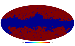
Figure 1: 60% sky mask used to compute the tSZ-X cross-power spectrum.

We also constructed a mask to avoid contamination by galactic or point source emissions in Planck data. Considering that the Planck 857 GHz channel is a good tracer of the thermal dust emission, we chose to mask all regions that present an emission above 3 $K_{\rm CMB}$ at this frequency (see Planck Collaboration results. IX, 2014, for unit convention and conversion). We masked all sources from the Planck compact source catalogue (Planck Collaboration results. XXVIII, 2014) detected in at least one frequency with a signal-to-noise ratio (S/N) above 5. We also masked all regions with an exposure of 0 seconds in the RASS survey. After applying these cuts, we kept about 60% of the sky for the analysis. We present the resulting mask in Fig. 1. We also considered masks of 20% and 40% for robustness checks with different thresholds for the thermal dust emission.

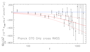
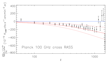
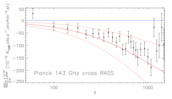
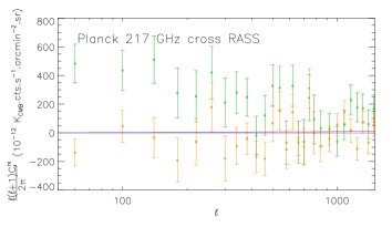
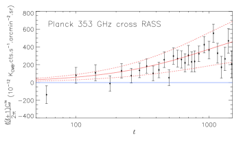
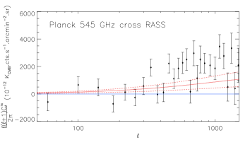
Figure 2: Cleaned cross-correlation power spectra between the RASS in the 0.5-2.0 keV energy band and the Planck frequency maps. From left to right and top to bottom we display spectra for 70, 100, 143, 217, 353 and 545 GHz. Data samples and error bars at 1 $\sigma$ are presented in black, the theoretical prediction using the Planck best-fitting cosmological parameters is plotted as a red solid line, the 1 $\sigma$ uncertainties on the theoretical prediction as estimated in Hurier et al. (2014) are depicted as red dashed lines, the cross-correlation at 217 GHz before CMB and dust subtraction is displayed in green, and the cross-correlation at 217 GHz only corrected for dust in orange. Uncertainties have been computed as presented in Eq. 13

.

We chose to exclude the Planck official CMB and foreground maps from the cleaning of frequency maps. This choice was motivated by the contamination of the Planck official CMB maps by tSZ residuals (see e.g. Bobin et al., 2014), which would bias our analysis. We also show in Sect. 4.1 that galactic foregrounds can be kept under control using thermal dust cleaning and a galactic mask. As a consequence, we did not perform CO (Planck Collaboration results. XIII, 2013) or low-frequency galactic emission (Planck Collaboration results. XII, 2014) cleaning, because it would have increased the noise level without significantly improving the results.

4 Dectecting the tSZ-Xray cross-correlation

The tSZ-X angular cross-power spectrum can be estimated from frequency maps or from a tSZ Compton parameter map. In this section, we explore the two approaches and discuss advantages and drawbacks of each of them.
In each case, we binned the power spectra and corrected the cross-spectra for beam and mask effects. The beam was corrected for by dividing the power-spectra by the beam transfer function in $\ell$ space. We deconvolved the power spectra by the mask-induced mixing matrix, which also accounts for the covered sky fraction. For a detailed description of the mask correction see Tristram et al. (2005).

4.1 Analysis for each frequency channel

We computed the angular cross-power spectrum, $C_{\ell}^{\nu,{\rm RASS}}$, between Planck frequency maps from $\nu=$ 70 to 857 GHz and the RASS full-sky map in the 0.5-2.0 keV energy band.

At a given frequency, the sky signal is dominated by CMB below 217 GHz and by thermal dust emission above 217 GHz.

We first corrected for CMB contamination by applying the transformation

$$\tilde{C}_{\ell}^{\nu,{\rm RASS}}=\frac{C_{\ell}^{\nu,{\rm RASS}}-C_{\ell}^{217,{\rm RASS}}}{1-f(217)/f(\nu)},$$ (9)

where $f(\nu)$ is the tSZ transmission in the Planck map at the frequency, $\nu$. The term $f(217)/f(\nu)$ is very small because the tSZ transmission in the Planck 217 GHz channel is almost null. This cleaning process prevents contamination at calibration uncertainty level (Planck Collaboration results. VIII, 2014) by processes that follow the same spectral energy distribution (SED) as the CMB black-body radiation (e.g. the kinetic SZ effect).
Then we corrected for thermal dust contamination by applying the transformation

$$\widehat{C}_{\ell}^{\nu,{\rm RASS}}=\frac{\tilde{C}_{\ell}^{\nu,{\rm RASS}}-\left(\rho_{857,\nu}-\rho_{857,217}\right)C_{\ell}^{857,{\rm RASS}}}{1-\left(\rho_{857,\nu}-\rho_{857,217}\right)f(857)/f(\nu)}.$$ (10)

The value of $\rho_{857,\nu}$ was estimated from a linear fit of the lowest multipoles of the power spectra of ($\ell<10$) because the thermal dust emission dominates the cross-power spectra at low multipoles. The factor $\left(\rho_{857,\nu}-\rho_{857,217}\right)f(857)/f(\nu)$ is negligible because of the ratio between tSZ and thermal dust SEDs at high frequencies. $\widehat{C}_{\ell}^{\nu,{\rm RASS}}$ spectra are referred to as the cleaned cross-power spectra in the following.

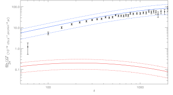
Figure 3: In black we present the cross-correlation power spectrum between the RASS in the 0.5-2.0 keV energy band map and the MILCA $y$-map computed from Planck data. As a dark blue solid line we show the theoretical one-halo tSZ-Xray cross-correlation power spectrum for Planck best-fitting cosmological parameters, in red the contribution of the two-halo term, and as dashed lines we show the 1 $\sigma$ uncertainties on the theoretical prediction as estimated in Hurier et al. (2014). Uncertainties have been computed as presented in Eq. 15.

.

In Fig. 2, we present the cleaned cross-power spectra between the RASS map and the Planck maps at 70, 100, 143, 353, and 545 GHz. We computed the $\chi^{2}$ of each spectrum compared to a null correlation. We obtain $\chi^{2}=86$, $274$, $378$, $205$, and $134$ for 31 degrees of freedom from $\ell=100$ to $\ell=2000$ at 70, 100, 143, 353, and 545 GHz, respectively. We also display the cross-correlation at 217 GHz without CMB and dust subtraction, and with dust correction alone. After dust correction, the cross-spectrum at 217 GHz is compatible with zero, with $\chi^{2}=30$ for 31 degree of freedom.
We compared these cross-spectra with the theoretical prediction assuming the Planck-CMB best-fitting $\Lambda$CDM cosmology ($\Omega_{\rm m}=0.3175$, $\sigma_{8}=0.8344$, and $H_{0}=67$ km/s/Mpc) (Planck Collaboration results. XVI, 2014). We observe a significant correlation that follows a tSZ SED. However, we note that the correlation signal appears to be significantly weaker than the prediction. We also note a significant contamination in the cross-power spectra at 100 and 143 GHz. This contamination can be seen at high multi-pole values ($\ell$ ¿ 1000) and is interpreted as a correlation between radio and X-ray AGNs that compensates the negative correlation between the tSZ and the X-ray emission from galaxy clusters at those frequencies.
The angular cross-power spectrum at 545 GHz significantly exceeds the theoretical prediction. This excess can be interpreted as a contamination by the correlation between X-ray emission and the cosmic infra-red background.
Figure 2 illustrates the main advantages of using a multi-frequency measurement of the tSZ-X cross-power spectrum. Indeed, with multi-frequency measurements, we can easily distinguish contamination sources from the tSZ-X signal by using the differences in SEDs.

4.2 Compton parameter map based analysis

We used a second approach to extract the tSZ-X cross-power spectrum. In this case, we built a tSZ Compton parameter map ($y$-map) using the MILCA method (Hurier et al., 2013) on the Planck maps from at 100 to 857 GHz. We verified that including frequencies from 30 to 70 GHz does not change the results.
The tSZ-X angular cross-power spectrum is obtained by directly cross-correlating the reprojected RASS full-sky map and the $y$-map, using 69% of the sky.

In Fig. 3, we present the derived cross-power spectrum and compare it with the theoretical prediction assuming the Planck-CMB best-fitting cosmology. We also computed the $\chi^{2}$ of the spectrum with respect to a null correlation. We derive $\chi^{2}=2687$ for 33 degrees of freedom from $\ell=50$ to $\ell=2000$. Similarly to the multi-frequency analysis, we observe that the measured power spectrum is significantly weaker than the prediction. However, the shape of the measured power spectrum agrees with the shape of the prediction. As the $y$-map reconstruction is performed both in pixel and frequency domains, it allows us to extract the tSZ signal at a higher S/N than a linear combination of power spectra. However, the identification and estimate of contamination sources is more complicated.
Consequently, the two approaches are complementary and were used together to check the robustness of the results.

4.3 Robustness of the detection

In this section we verify that our signal is produced by galaxy cluster and not by AGNs.

We estimated the contamination from known AGN using X-ray catalogues such as the ROSAT Bright Survey (RBS, Fischer et al., 1998). First, we projected the RBS sources on a full-sky map. We computed the cross-spectrum between the $y$-map and the projected RBS map considering only sources flagged as AGNs. Then, we performed the same analysis for sources flagged as clusters. Uncertainties were computed following the approach presented in Sect. 5.1. We present the obtained cross-spectra in Fig. 4. We do not observe any significant contribution from this AGNs sample. These spectra illustrate that our signal is dominated by X-ray emission from galaxy clusters and not from X-ray AGNs.

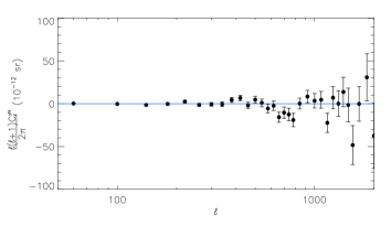
Figure 4: Top panel: cross-spectrum between the MILCA $y$-map and the RBS sources flagged as AGN (black samples), the blue line shows the 0 correlation. Bottom panel: cross-spectrum between the MILCA $y$-map and the RBS sources flagged as galaxy clusters.

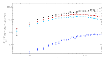
Figure 5: In black we present the cross-correlation power spectrum between the RASS in the 0.5-2.0 keV energy range map and the MILCA $y$-map computed from Planck data, in red the contribution from all clusters in the MCXC catalogue (Piffaretti et al., 2011), in light blue the contribution from all known clusters in the PSZ catalogue (Planck Collaboration results. XXIX, 2014), and in dark blue the contribution from the Planck cosmo sample used in (Planck Collaboration results. XX, 2014).

We also estimated the contribution of known tSZ and X-ray galaxy clusters to the tSZ-X cross-power spectrum. To do so, we built several tSZ maps for different subsamples of galaxy clusters. We considered the Planck SZ catalogue (Planck Collaboration early results. VIII, 2011; Planck Collaboration results. XXIX, 2014), the Planck cosmo sample (Planck Collaboration results. XX, 2014), and the MCXC (Piffaretti et al., 2011).
For the Planck SZ catalogue we used confirmed galaxy clusters (861 clusters) with fluxes $Y_{500}$ and radius $R_{500}$ estimated from 2D likelihoods provided in Planck Collaboration results. XXIX (2014) and a universal pressure profile (Arnaud et al., 2010). For X-rays clusters, we predicted the tSZ flux assuming a scaling relation between $Y_{500}$ and $L_{500}$ from Planck Collaboration early results. XI (2011) and X-ray deduced values for $R_{500}$.
We projected each cluster on an oversampled grid with a pixel size of 0.1$\times\theta_{500}$ (e.g. drizzling) to avoid flux loss during the projection. Then we convolved the oversampled map with a beam FWHM of 10 arc minutes. We reprojected the oversampled map on a HEALpix full-sky map with 1.7 arc minute pixels using a nearest-neighbour interpolation.

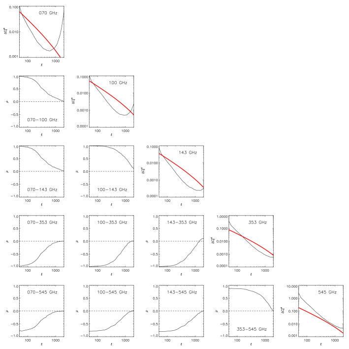
Figure 6: Diagonal figures show in black the uncertainty level for $C_{\ell}^{\nu,RASS}$ in units of K${}_{\rm CMB}.$cts.s^-1.armin^-2.sr for the cleaned power spectra between the RASS map in the 0.5-2.0 keV energy range and the Planck maps at 70, 100, 143, 353, and 545 GHz, using a binning of $\Delta\ell=40$, In red we show the tSZ-Xray cross-power spectrum for the model. The off diagonal figures show the correlation factor $\rho$ between $C_{\ell}^{yx}$ at frequencies $\nu$ and $\nu^{\prime}$. See Sect. 5.1 for details on computing uncertainties and their covariance.

Then, we computed the angular cross-power spectrum between the tSZ template maps and the ROSAT full-sky count-rate map. Uncertainties were computed following the approach presented in in Sect. 5.1.
In Fig. 5, we present the derived angular power spectra for each sample of clusters. The known X-ray clusters from the MCXC contribute about 75% of the total power at low-$\ell$ ($\ell<800$). Confirmed Planck tSZ clusters contribute about 50% of the power of the tSZ-X spectrum at low-$\ell$ ($\ell<800$). The Planck cosmo sample contributes about 1% at low-$\ell$.
Known clusters contribute essentially at low-$\ell$. At high-$\ell$, the tSZ-X spectrum presents contribution from low-mass and high-$z$ galaxy clusters. Planck -confirmed clusters and MCXC clusters only contribute 20% and 40% of the total power at $\ell=2000$, as expected considering the contribution from undetected galaxy clusters.
These spectra demonstrate that the full tSZ-X cross-power spectrum contains additional informations on cosmology relevant to tSZ number count studies.

5 Estimating bias and uncertainties

We discuss in detail the main sources of uncertainties and biases in the measurement of the tSZ-X cross-power spectrum.

5.1 Statistical uncertainties

The cleaned angular cross-power spectra are constructed using a linear combination of three cross-power spectra, $C_{\ell}^{\nu,{\rm RASS}}$, at different frequencies, see Sect. 4.1. Consequently, we need to estimate variances and covariances of these spectra. The variance, ${\rm var}(\nu)$, of $C_{\ell}^{\nu,{\rm RASS}}$ can be expressed as

$${\rm var}(\nu)=\frac{1}{(2\ell+1)f_{\rm sky}}\left[\left(C_{\ell}^{\nu,{\rm RASS}}\right)^{2}+C_{\ell}^{\nu,\nu}C_{\ell}^{{\rm RASS},{\rm RASS}}\right],$$ (11)

and the covariance, ${\rm cov}(\nu,\nu^{\prime})$, between $C_{\ell}^{\nu,{\rm RASS}}$ and $C_{\ell}^{\nu^{\prime},{\rm RASS}}$ reads

$${\rm cov}(\nu,\nu^{\prime})=\frac{1}{(2\ell+1)f_{\rm sky}}\left[C_{\ell}^{\nu,{\rm RASS}}C_{\ell}^{\nu^{\prime},{\rm RASS}}+C_{\ell}^{\nu,\nu^{\prime}}C_{\ell}^{{\rm RASS},{\rm RASS}}\right].$$ (12)

Then, the variance of $\widehat{C}_{\ell}^{\nu,{\rm RASS}}$ can be computed as

$${\rm var}(\widehat{\nu})= \,{\rm var}(\nu)+{\rm var}(217)+\left(\rho_{857,\nu}-\rho_{857,217}\right)^{2}{\rm var}(857)$$

$$-2\left(\rho_{857,\nu}-\rho_{857,217}\right)\left[{\rm cov}(\nu,857)-2{\rm cov}(217,857)\right]$$

$$-2{\rm cov}(\nu,217).$$ (13)

It can be useful to combine constraints from the different cleaned power spectra. To do so, we computed the covariance between $\widehat{C}_{\ell}^{\nu,{\rm RASS}}$ and $\widehat{C}_{\ell}^{\nu^{\prime},{\rm RASS}}$ as

$${\rm cov}(\widehat{\nu},\widehat{\nu^{\prime}})= \,{\rm cov}(\nu,\nu^{\prime})+{\rm var}(217)$$

$$+\left(\rho_{857,\nu}-\rho_{857,217}\right)\left(\rho_{857,\nu^{\prime}}-\rho_{857,217}\right){\rm var}(857)$$

$$-{\rm cov}(\nu,217)-{\rm cov}(\nu^{\prime},217)$$

$$-\left(\rho_{857,\nu}-\rho_{857,217}\right)\left[{\rm cov}(\nu,857)-{\rm cov}(217,857)\right]$$

$$-\left(\rho_{857,\nu^{\prime}}-\rho_{857,217}\right)\left[({\rm cov}(\nu^{\prime},857)-{\rm cov}(217,857)\right].$$

We propagated the whole covariance matrix through binning and mask deconvolution processes. In Fig. 6, we present the uncertainties on $\widehat{C}_{\ell}^{\nu,{\rm RASS}}$ and the correlation factor between $\widehat{C}_{\ell}^{\nu,{\rm RASS}}$ and $\widehat{C}_{\ell}^{\nu^{\prime},{\rm RASS}}$ for the cleaned cross-power spectra at 70, 100, 143, 353, and 545 GHz.
In this figure and in the diagonal plots, we observe that at low frequencies the uncertainty level increases with the multipole. This is produced by the deconvolution from the instrumental resolution. We observe a flattening in the uncertainty level at high-$\ell$ for the highest frequencies. This flattening indicates that the signal is dominated by the instrumental noise.
At low-$\ell$ the correlation factors are close to 1 or -1, indicating an almost total correlation between uncertainties below $\ell=100$ at 70, 100, 143, and 353 GHz. This indicates that the uncertainties at these multipole values are dominated by cosmic variance of the tSZ-X cross-spectrum.
The instrumental noise domination at high-$\ell$ also appears in the correlation factor between frequencies. When the noise dominates the uncertainty budget, these coefficients become zero.

For a tSZ-X power spectrum estimated from a $y$-map, the variance, ${\rm var}(y)$, can be directly estimated as

$${\rm var}(y)=\frac{1}{(2\ell+1)f_{\rm sky}}\left[\left(C_{\ell}^{y,{\rm RASS}}\right)^{2}+C_{\ell}^{y,y}C_{\ell}^{{\rm RASS},{\rm RASS}}\right].$$ (15)

The MILCA method is tailored to minimize instrumental noise and the variance of other astrophysical emissions, therefore we derive lower uncertainties (Fig. 3) than using the previous approach (Fig. 2).
We also probate these uncertainty through the binning and mask deconvolution processes.

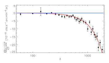
Figure 7: Estimating the AGN contamination to the MILCA-RASS angular cross-power spectrum using NVSS and SUMSS catalogues as tracers of radio-loud AGNs. Black samples show our estimates, the solid blue line shows the 0 level, and the solid red line shows the best-fit of this contamination.

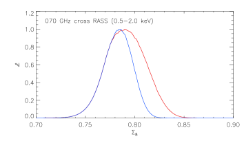
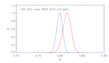
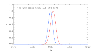
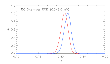
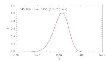
Figure 8: From left to right and top to bottom: likelihood functions of $\Sigma_{8}$ estimated from the angular cross-power spectra at 70, 100, 143, 353, and 545 GHz, respectively. This adjustment accounts for AGNs and CIB contaminations. Considering modelling from Eq. 17 in blue and from Eq. 18 in red.

5.2 Bias sources

There are several possible sources of bias in the tSZ-X cross-power spectrum. The thermal dust emission from the Milky Way can produce bias because it is correlated with the $n_{(H)}$ absorption of the X-rays. By masking the galactic plane and considering X-rays in the range [0.5,2.0] keV, we ensure that this bias is under control (see Morrison & McCammon, 1983, for absorption cross-sections). We have tested several galactic cuts (20, 40, and 60%) and found no significant variations in our measure (below 0.2 $\sigma$ on the tSZ-X cross-power spectra). This bias can thus be safely neglected.

There are also sources of biases that are correlated with the cluster spatial distribution over the sky. Indeed, all extra-galactic emissions are correlated with the matter distribution. On the X-ray side, we have mainly two components, the X-ray emission from clusters and from AGNs (noted AGN_X hereafter). On the microwave side, we have the tSZ effect, the radio emission from AGNs (noted AGN_R hereafter), and the cosmic infra-red background (CIB). Consequently, we have five cross-spectra from extra-galactic objects that can bias the measurement.
The extrapolated radio emission from AGNs is weak at Planck frequencies (e.g. Planck Collaboration results. XXIX, 2014), thus it does not produce a significant bias. In addition, the small number of un-masked high-flux X-ray AGNs prevents a significant contamination in terms of tSZ-AGN_X correlation. As a consequence, we considered that tSZ-AGN_X, AGN_R-X, and CIB-AGN_X cross-correlations are weaker than the AGN_R-AGN_X correlations. This leaves the tSZ-X, AGN_R-AGN_X, and CIB-X correlations as potentially significant contributions for the microwave-X correlation.

For the multi-frequency estimation of the tSZ-X correlation (see Sect. 4.1), this sources of bias can be separated from the tSZ-X signal using their SED. However, this is not possible in the $y$-map approach (see Sect. 4.2). To estimate the AGN-AGN level of contamination in the tSZ-X angular cross-power obtained from the reprojected RASS full sky map and the $y$-map, we assumed that radio catalogues are accurate tracers of the AGN population that may bias our measurement.

The NRAO VLA Sky Survey (NVSS) (Condon et al., 1998) is a 1.4 GHz continuum survey covering the entire sky north of Dec$\leavevmode\nobreak\ >-40^{\circ}$. The associated catalogue of discrete sources contains over 1.8 million radio sources. South of Dec$\leavevmode\nobreak\ <-30^{\circ}$ and at galactic latitudes $|b|>10^{\circ}$, the Sydney University Molonglo Sky Survey (SUMSS) (Mauch et al., 2003, 2008) is a 843 MHz continuum survey also providing a radio source catalogue. SUMSS and NVSS have similar sensitivities and angular resolutions, and combined, they cover the whole sky.
We extrapolated the SUMSS sources at 1.4 GHz assuming a spectral index of -1 in intensity units. Then, we built a map of NVSS sources weighted by their flux and filled the region Dec$\leavevmode\nobreak\ >-40^{\circ}$ with extrapolated SUMSS sources. We computed the cross-power spectra between the radio-sources map and the $y$-map, $C_{\ell}^{y,{\rm rad}}$ , and the RASS full-sky map, $C_{\ell}^{{\rm RASS},{\rm rad}}$.
Thus, we computed the estimate of the AGN-AGN contamination in the $C_{\ell}^{y,{\rm RASS}}$ spectrum as

$$C_{\ell}^{{\rm AGN}_{\rm R},{\rm AGN}_{\rm X}}=\frac{C_{\ell}^{y,{\rm rad}}C_{\ell}^{{\rm RASS},{\rm rad}}}{C_{\ell}^{{\rm rad},{\rm rad}}}.$$ (16)

In Fig. 7 we present the derived $C_{\ell}^{{\rm AGN}_{\rm R},{\rm AGN}_{\rm X}}$ spectrum. We fitted $C_{\ell}^{{\rm AGN}_{\rm R},{\rm AGN}_{\rm X}}$ with a constant considering that AGN are point-like sources. Neglecting their clustering, we derive $C_{\ell}^{{\rm AGN}_{\rm R},{\rm AGN}_{\rm X}}=(-46.6\pm 3.1)\,10^{-18}$ cts.s^-1.arcmin².sr (red line in Fig. 7).
Finally, we corrected the $y$-RASS cross-spectrum for this bias and propagated the related uncertainties.

Table 2: Best-fitting values for $\Sigma_{8}$ for different data subsets. From left to right: mean value of $\Sigma_{8}$, value of $\Sigma_{8}$ at the maximum likelihood, standard deviation of $\Sigma_{8}$, 68% interval, systematic uncertainties, and $\chi^{2}$ per degree of freedom.

Dataset	Model	$<\Sigma_{8}>$	$\Sigma_{8,max}$	$\sqrt{<{\Sigma_{8}}^{2}>-<{\Sigma_{8}}>^{2}}$	68% interval	$\Delta$ Syst	$\chi^{2}_{\rm ndf}$
X-rays $\times$ 70-545 GHz	Eq. 18	0.804	0.805	0.006	0.800 - 0.809	0.001	1.22
X-rays $\times$ 70 GHz	Eq. 17	0.782	0.784	0.015	0.770 - 0.798	0.020	1.51
X-rays $\times$ 100 GHz	Eq. 17	0.798	0.799	0.007	0.793 - 0.805	0.010	0.94
X-rays $\times$ 143 GHz	Eq. 17	0.799	0.799	0.006	0.794 - 0.804	0.010	1.24
X-rays $\times$ 353 GHz	Eq. 17	0.815	0.816	0.008	0.809 - 0.823	0.015	0.61
X-rays $\times$ 70 GHz	Eq. 18	0.791	0.790	0.020	0.771 - 0.809	0.001	1.51
X-rays $\times$ 100 GHz	Eq. 18	0.815	0.816	0.010	0.807 - 0.824	0.001	0.85
X-rays $\times$ 143 GHz	Eq. 18	0.806	0.806	0.007	0.800 - 0.812	0.001	1.20
X-rays $\times$ 353 GHz	Eq. 18	0.808	0.809	0.008	0.801 - 0.816	0.001	0.61
X-rays $\times$ 545 GHz	Eq. 18	0.803	0.808	0.018	0.790 - 0.822	0.001	1.35
X-rays $\times$ $y$-map	Eq. 19	0.804	0.804	0.003	0.801 - 0.806	0.002	1.15

6 Constraints

We explored three approaches to set cosmological constraints using the measurement of the tSZ-X cross-power spectrum. First, we considered individual frequencies, neglecting all sources of bias. Then, we considered the constraint from each frequency considering a multi-frequency adjustment for the biases. Finally, we considered the cross-spectrum with the tSZ $y$-map. In the following, we fit the data considering $\ell$ from 50 to 2000. We computed the likelihood functions assuming Gaussian uncertainties over a grid for $\Omega_{m}$, $\sigma_{8}$, and $H_{0}$, considering fixed values for other parameters. Then, we marginalized the likelihood to express it as a function of the degeneracy relation between parameters, $\Sigma_{8}$. For cosmological constraints, we used fixed values of $a_{\rm x}$ and $a_{\rm sz}$ and propagated the uncertainties on these values to $\Sigma_{8}$. In the following, uncertainties are given for 68% confidence level. We verified that we derived compatible results within the error bars using different galactic masks (see Sect. 3). This demonstrates that our results are not significantly affected by galactic foreground contamination.

6.1 Cosmological constraints per frequency channel

Considering a single-frequency approach, we estimated $\Sigma_{8}$ for each frequency individually, excluding 545 GHz, which is contaminated. We assumed the model

$$\widehat{C}_{\ell}^{\nu,{\rm RASS}}=g(\nu)C_{\ell}^{yx}(\Sigma_{8}^{\nu}).$$ (17)

The derived likelihoods are presented in Fig. 8 and the best-fitting values are summarized in Table. 2. Our best-fitting values for $\Sigma_{8}^{\nu}$ increase with frequency with this simple modelling. This behaviour is produced by the contamination of AGN and CIB. The radio-loud AGNs produce an excess of correlation at low frequency that compensates for the anti-correlation between tSZ and X-ray emission. At high frequency, the CIB-X correlation produces an excess of correlation that biases the correlation between tSZ and X-ray emission. The values deduced from spectra at 100 GHz agree well with those at 143 GHz, which present the lowest bias level.

6.2 Cosmological constraints from the multi-frequency approach

To prevent contamination produced by AGNs and CIB in the fit, we modelled the measured spectra, $\widehat{C}_{\ell}^{\nu,{\rm RASS}}$, as follows:

$$\widehat{C}_{\ell}^{\nu,{\rm RASS}}=\left[g(\nu)+A_{\rm CIB}f_{\rm CIB}(\nu)\right]C_{\ell}^{yx}(\Sigma_{8}^{\nu})+A_{\rm rad}f_{\rm rad}(\nu),$$ (18)

where $f_{\rm CIB}$ (Gispert et al., 2000) and $f_{\rm rad}(\nu)$ (Planck Collaboration Int. results. VII, 2013) are fixed SED for CIB and radio-loud AGN contaminations.
Given the large uncertainties at 545 GHz for the tSZ-X cross-correlation measurement, the signal is not sensitive to the shape of the CIB-X correlation. Therefore and for simplicity, we assumed that the CIB-X angular cross-power spectrum has the same shape, with respect to $\ell$, as the tSZ-X cross-correlation.
We fitted for $A_{\rm rad}$, $A_{\rm CIB}$ and $\Sigma_{8}^{\nu}$ the amplitude of the radio and CIB contamination and the tSZ-X angular cross-power spectrum degenerate amplitude defined in Eq. 8. Parameters $A_{\rm rad}$ and $A_{\rm CIB}$ were fitted using the five frequencies 70, 100, 143, 353, and 545 GHz; $\Sigma_{8}^{\nu}$ was fitted individually for each frequency.
The derived likelihoods are presented in Fig. 8. Best-fitting values are summarized in Table. 2. The $\Sigma_{8}$ values now agree well, including the value deduced from the 545 GHz spectra. There is no significant frequency dependence for $\Sigma_{8}$, indicating that our modelling accounts properly for contamination by other astrophysical components.

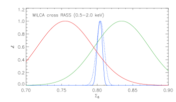
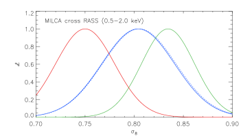
Figure 9: Top panel: constraints on $\Sigma_{8}$. Bottom panel: associated constraints on $\sigma_{8}$ considering the modelling uncertainties. The solid dark blue line depicts the likelihood functions estimated from the angular cross-power spectra between the MILCA and the ROSAT full-sky maps. The dashed dark blue line represents the likelihood function estimated from the cleaned cross-power spectra at 70, 100, 143, 353, and 545 GHz. This adjustment accounts for AGN contamination. In red we show the constraints considering the cosmology from the cluster number count, in green the constraints considering the cosmology from Planck-CMB.

Then, we adjusted $\Sigma_{8}$ using the model presented in Eq. 18 and all frequencies simultaneously. Figure 9 presents the likelihood function for $\Sigma_{8}$ and $\sigma_{8}$. We obtain a best-fit value of $\Sigma_{8}=0.804\pm 0.006\pm 0.001$, with statistical and systematic uncertainties, respectively, where systematic uncertainties account for residual contamination.
We estimated the expected value for $\Sigma_{8}$ considering the cosmological constraints from analyses based on CMB (Planck Collaboration results. XVI, 2014) and cluster counts (Planck Collaboration results. XX, 2014). Cluster number counts and CMB power spectra present different degeneracies for cosmological parameters from those of tSZ-X cross-spectrum. This leads to large error bars when $\Sigma_{8}$ is estimated from cluster counts or CMB. Uncertainty levels derived assuming cluster number count and CMB cosmology are described in Hurier et al. (2014).
We stress that these uncertainties are not representative of the uncertainties on $\sigma_{8}$. We need to propagate the uncertainty on the modelling parameters to $\sigma_{8}$. Consequently, the constraints on cosmological parameters read $\sigma_{8}\left[\left(\frac{\Omega_{m}}{0.3175}\right)^{3.42}\left(\frac{H_{0}}{67}\right)^{2.36}\right]^{\frac{1}{8.12}}=0.805\pm 0.006\pm 0.001\pm 0.025,$ with statistical, systematic, and modeling uncertainties, respectively. The constraint on $\sigma_{8}$ gives $\sigma_{8}=0.805\pm 0.037.$ We observe that the error budget is dominated by modelling uncertainties.

6.3 Cosmological constraints from a $y$-map

We estimated the level of CIB-X contamination in the $y$-RASS power spectrum by propagating the $A_{\rm CIB}$ amplitude through the MILCA linear weights. We deduce that this contamination is negligible. Indeed, the CIB only contaminates the tSZ-X correlation at high frequency, where the weights are smaller than at low frequencies.

To reproduce the $y$-RASS spectrum, we assumed the following modedling:

$$C_{\ell}^{y,{\rm RASS}}=C_{\ell}^{yx}(\Sigma_{8})+A_{\rm rad},$$ (19)

where $A_{\rm rad}$ is estimated as presented in Sect. 2. From this measurement, we obtain $\sigma_{8}\left[\left(\frac{\Omega_{m}}{0.3175}\right)^{3.42}\left(\frac{H_{0}}{67}\right)^{2.36}\right]^{\frac{1}{8.12}}=0.804\pm 0.003\pm 0.002\pm 0.025$ and $\sigma_{8}=0.804\pm 0.037$.

In Fig. 9, we present the likelihood for $\Sigma_{8}$ and $\sigma_{8}$ . The constraints on $\Sigma_{8}$ derived from the tSZ-X power spectrum are consistent with predictions from cluster counts and CMB. Moreover, the constraints derived from the $y$-map are consistent with constraints derived from the multi-frequency analysis presented in Sect. 6.2.

6.4 Constraints on scaling-law parameters

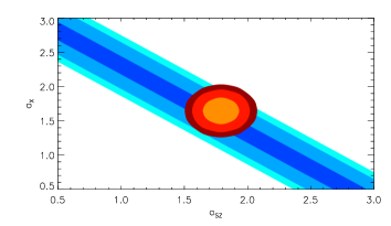
Figure 10: Two-dimensional likelihood function for the scaling relation mass power-laws, $a_{\rm sz}$ and $a_{\rm x}$. In blue we present the 1, 2 and, 3 $\sigma$ confidence levels from our measurement of the tSZ-X cross-spectrum, in red the 1, 2 and 3 $\sigma$ confidence levels for our constraints on the scaling-law mass indices.

In Fig. 10, we present the constraints on the scaling relation power-law indices from combined tSZ-X and tSZ-tSZ power spectra. We assumed a fixed pressure profile (best-fit on a GNFW profile from Arnaud et al., 2010) and polytropic index of 1.5 for galaxy clusters.
From the tSZ-Xray cross-spectrum, we derive $a_{\rm sz}+a_{\rm x}=3.37\pm 0.09$, which is to be compared with $a_{\rm sz}+a_{\rm x}=3.43\pm 0.15$ when considering values listed in Table. 1. Figure 10 shows that constraints from the tSZ-X spectrum alone are consistent with previous constraints (see e.g. Pratt et al., 2009; Planck Collaboration early results. XI, 2011) on $a_{\rm x}$ and $a_{\rm sz}$ .

To explore the possible evolution of the scaling relations with redshift, we assumed a power-law dependence of the form $(1+z)^{\beta}$. Then, we fitted for $\beta_{\rm sz}+\beta_{\rm x}$ the tSZ and X-ray evolution indices. We derive $\beta_{\rm sz}+\beta_{\rm x}=0.4^{+0.4}_{-0.5}$ from the tSZ-X angular cross-power spectrum.

We stress that the constraints on scaling-law indices are degenerate with the assumed density and temperature profiles for galaxy clusters (as discussed in Hurier et al., 2014).

7 Conclusion

We have performed the first detection of the tSZ-X angular cross-power spectrum directly estimated from X-ray count rate and tSZ signal. We detected a clearly correlated emission between tSZ-map and X-ray count-rate map in the range $50<\ell<2000$ at an overall significance of 28 $\sigma$.
We accounted for statistical systematics from residuals (mainly AGN and CIB) and for modelling uncertainties.

Using the amplitude of the tSZ-X angular cross-power spectrum, we derived constraints on cosmological parameters $\sigma_{8}\left[\left(\frac{\Omega_{m}}{0.3175}\right)^{3.42}\left(\frac{H_{0}}{67}\right)^{2.36}\right]^{\frac{1}{8.12}}=0.804\pm 0.003\pm 0.002\pm 0.025$ with statistical, systematic, and modelling uncertainties. These constraints read $\sigma_{8}=0.804\pm 0.037$ if we consider $\Omega_{m}$ from Planck-CMB best-fit cosmology (Planck Collaboration results. XVI, 2014). We tested the robustness of this result using an analysis based on multiple frequencies and on a tSZ-map.
With a mass bias of 0.2, this result is compatible with constraints based on cluster count and CMB on $\sigma_{8}$ from Planck Collaboration results. XX (2014) and Planck Collaboration results. XVI (2014). This constraint is also consistent with the cross-correlation measured by Hajian et al. (2013) between the tSZ emission and an X-ray sample of galaxy clusters and with the X-ray cluster number count (Vikhlinin et al., 2009; Böhringer et al., 2014).

Using the shape of the tSZ-X cross-spectrum, we were able to constrain the scaling-law mass and evolution indices of $L_{500}-M_{500}$ and $Y_{500}-M_{500}$. We derived $a_{\rm sz}+a_{\rm x}=3.37\pm 0.09$ and $\beta_{\rm sz}+\beta_{\rm x}=0.4^{+0.4}_{-0.5}$. Consistently with previous results from Reichert et al. (2011) for the X-ray scaling relation, we found that the redshift evolution of the scaling law is consistent with self-similar evolution.

References

- Abell et al. (1989) Abell, G. O., Corwin, Jr., H. G., & Olowin, R. P. 1989, ApJS, 70, 1
- Afshordi et al. (2007) Afshordi, N., Lin, Y.-T., Nagai, D., & Sanderson, A. J. R. 2007, MNRAS, 378, 293
- Afshordi et al. (2005) Afshordi, N., Lin, Y.-T., & Sanderson, A. J. R. 2005, ApJ, 629, 1
- Arnaud et al. (2010) Arnaud, M., Pratt, G. W., Piffaretti, R., et al. 2010, A&A, 517, A92
- Atrio-Barandela et al. (2008) Atrio-Barandela, F., Kashlinsky, A., Kocevski, D., & Ebeling, H. 2008, ApJ, 675, L57
- Bennett et al. (2003) Bennett, C. L., Hill, R. S., Hinshaw, G., et al. 2003, ApJS, 148, 97
- Benson et al. (2013) Benson, B. A., de Haan, T., Dudley, J. P., et al. 2013, ApJ, 763, 147
- Bleem et al. (2014) Bleem, L. E., Stalder, B., de Haan, T., et al. 2014, ArXiv e-prints
- Bobin et al. (2014) Bobin, J., Sureau, F., Starck, J.-L., Rassat, A., & Paykari, P. 2014, A&A, 563, A105
- Böhringer et al. (2014) Böhringer, H., Chon, G., & Collins, C. A. 2014, ArXiv e-prints
- Böhringer et al. (2001) Böhringer, H., Schuecker, P., Guzzo, L., et al. 2001, A&A, 369, 826
- Bohringer et al. (2000) Bohringer, H., Voges, W., Huchra, J. P., et al. 2000, VizieR Online Data Catalog, 212, 90435
- Cole & Kaiser (1988) Cole, S. & Kaiser, N. 1988, MNRAS, 233, 637
- Condon et al. (1998) Condon, J. J., Cotton, W. D., Greisen, E. W., et al. 1998, AJ, 115, 1693
- Diego & Majumdar (2004) Diego, J. M. & Majumdar, S. 2004, MNRAS, 352, 993
- Diego & Partridge (2010) Diego, J. M. & Partridge, B. 2010, MNRAS, 402, 1179
- Diego et al. (2003) Diego, J. M., Silk, J., & Sliwa, W. 2003, MNRAS, 346, 940
- Dunkley et al. (2011) Dunkley, J., Hlozek, R., Sievers, J., et al. 2011, ApJ, 739, 52
- Ebeling et al. (2000) Ebeling, H., Edge, A. C., Allen, S. W., et al. 2000, VizieR Online Data Catalog, 731, 80333
- Ebeling et al. (2001) Ebeling, H., Edge, A. C., & Henry, J. P. 2001, ApJ, 553, 668
- Fischer et al. (1998) Fischer, J.-U., Hasinger, G., Schwope, A. D., et al. 1998, Astronomische Nachrichten, 319, 347
- Fosalba et al. (2003) Fosalba, P., Gaztañaga, E., & Castander, F. J. 2003, ApJ, 597, L89
- Gispert et al. (2000) Gispert, R., Lagache, G., & Puget, J. L. 2000, A&A, 360, 1
- Gladders & Yee (2005) Gladders, M. D. & Yee, H. K. C. 2005, ApJS, 157, 1
- Górski et al. (2005) Górski, K. M., Hivon, E., Banday, A. J., et al. 2005, ApJ, 622, 759
- Hajian et al. (2013) Hajian, A., Battaglia, N., Spergel, D. N., et al. 2013, ArXiv e-prints
- Hasselfield et al. (2013) Hasselfield, M., Hilton, M., Marriage, T. A., et al. 2013, J. Cosmology Astropart. Phys., 7, 8
- Hernández-Monteagudo et al. (2004) Hernández-Monteagudo, C., Genova-Santos, R., & Atrio-Barandela, F. 2004, ApJ, 613, L89
- Hernández-Monteagudo et al. (2006) Hernández-Monteagudo, C., Macías-Pérez, J. F., Tristram, M., & Désert, F.-X. 2006, A&A, 449, 41
- Hinshaw et al. (2007) Hinshaw, G., Nolta, M. R., Bennett, C. L., et al. 2007, ApJS, 170, 288
- Hurier et al. (2014) Hurier, G., Aghanim, N., & Douspis, M. 2014, A&A, 568, A57
- Hurier et al. (2013) Hurier, G., Macías-Pérez, J. F., & Hildebrandt, S. 2013, A&A, 558, A118
- Kalberla et al. (2005) Kalberla, P. M. W., Burton, W. B., Hartmann, D., et al. 2005, A&A, 440, 775
- Koester et al. (2007) Koester, B. P., McKay, T. A., Annis, J., et al. 2007, ApJ, 660, 239
- Komatsu & Kitayama (1999) Komatsu, E. & Kitayama, T. 1999, ApJ, 526, L1
- Komatsu & Seljak (2002) Komatsu, E. & Seljak, U. 2002, MNRAS, 336, 1256
- Komatsu et al. (2011) Komatsu, E., Smith, K. M., Dunkley, J., et al. 2011, ApJS, 192, 18
- Lieu et al. (2006) Lieu, R., Mittaz, J. P. D., & Zhang, S.-N. 2006, ApJ, 648, 176
- Marriage et al. (2011) Marriage, T. A., Acquaviva, V., Ade, P. A. R., et al. 2011, ApJ, 737, 61
- Mauch et al. (2003) Mauch, T., Murphy, T., Buttery, H. J., et al. 2003, MNRAS, 342, 1117
- Mauch et al. (2008) Mauch, T., Murphy, T., Buttery, H. J., et al. 2008, VizieR Online Data Catalog, 8081, 0
- Melin et al. (2011) Melin, J.-B., Bartlett, J. G., Delabrouille, J., et al. 2011, A&A, 525, A139
- Mewe et al. (1985) Mewe, R., Gronenschild, E. H. B. M., & van den Oord, G. H. J. 1985, A&AS, 62, 197
- Mo & White (1996) Mo, H. J. & White, S. D. M. 1996, MNRAS, 282, 347
- Morrison & McCammon (1983) Morrison, R. & McCammon, D. 1983, ApJ, 270, 119
- Myers et al. (2004) Myers, A. D., Shanks, T., Outram, P. J., Frith, W. J., & Wolfendale, A. W. 2004, MNRAS, 347, L67
- Piffaretti et al. (2011) Piffaretti, R., Arnaud, M., Pratt, G. W., Pointecouteau, E., & Melin, J.-B. 2011, A&A, 534, A109
- Planck Collaboration early results. VIII (2011) Planck Collaboration early results. VIII. 2011, A&A, 536, A8
- Planck Collaboration early results. X (2011) Planck Collaboration early results. X. 2011, A&A, 536, A10
- Planck Collaboration early results. XI (2011) Planck Collaboration early results. XI. 2011, A&A, 536, A11
- Planck Collaboration Int. results. VII (2013) Planck Collaboration Int. results. VII. 2013, A&A, 550, A133
- Planck Collaboration results. I (2014) Planck Collaboration results. I. 2014, A&A, 571, A1
- Planck Collaboration results. IX (2014) Planck Collaboration results. IX. 2014, A&A, 571, A9
- Planck Collaboration results. VII (2014) Planck Collaboration results. VII. 2014, A&A, 571, A7
- Planck Collaboration results. VIII (2014) Planck Collaboration results. VIII. 2014, A&A, 571, A8
- Planck Collaboration results. XII (2014) Planck Collaboration results. XII. 2014, A&A, 571, A12
- Planck Collaboration results. XIII (2013) Planck Collaboration results. XIII. 2013, e-prints ArXiv: 1303.5073
- Planck Collaboration results. XVI (2014) Planck Collaboration results. XVI. 2014, A&A, 571, A16
- Planck Collaboration results. XX (2014) Planck Collaboration results. XX. 2014, A&A, 571, A20
- Planck Collaboration results. XXI (2014) Planck Collaboration results. XXI. 2014, A&A, 571, A21
- Planck Collaboration results. XXIX (2014) Planck Collaboration results. XXIX. 2014, A&A, 571, A29
- Planck Collaboration results. XXVIII (2014) Planck Collaboration results. XXVIII. 2014, A&A, 571, A28
- Pratt et al. (2009) Pratt, G. W., Croston, J. H., Arnaud, M., & Böhringer, H. 2009, A&A, 498, 361
- Reichardt et al. (2012) Reichardt, C. L., Shaw, L., Zahn, O., et al. 2012, ApJ, 755, 70
- Reichert et al. (2011) Reichert, A., Böhringer, H., Fassbender, R., & Mühlegger, M. 2011, A&A, 535, A4
- Rykoff et al. (2013) Rykoff, E. S., Rozo, E., Busha, M. T., et al. 2013, ArXiv e-prints
- Sehgal et al. (2011) Sehgal, N., Trac, H., Acquaviva, V., et al. 2011, ApJ, 732, 44
- Shirokoff et al. (2011) Shirokoff, E., Reichardt, C. L., Shaw, L., et al. 2011, ApJ, 736, 61
- Sievers et al. (2013) Sievers, J. L., Hlozek, R. A., Nolta, M. R., et al. 2013, J. Cosmology Astropart. Phys., 10, 60
- Sunyaev & Zeldovich (1969) Sunyaev, R. A. & Zeldovich, Y. B. 1969, Nature, 223, 721
- Sunyaev & Zeldovich (1972) Sunyaev, R. A. & Zeldovich, Y. B. 1972, Comments on Astrophysics and Space Physics, 4, 173
- Taburet et al. (2011) Taburet, N., Hernández-Monteagudo, C., Aghanim, N., Douspis, M., & Sunyaev, R. A. 2011, MNRAS, 418, 2207
- The Dark Energy Survey Collaboration (2005) The Dark Energy Survey Collaboration. 2005, ArXiv Astrophysics e-prints
- Tinker et al. (2008) Tinker, J., Kravtsov, A. V., Klypin, A., et al. 2008, ApJ, 688, 709
- Tristram et al. (2005) Tristram, M., Macías-Pérez, J. F., Renault, C., & Santos, D. 2005, MNRAS, 358, 833
- Vanderlinde et al. (2010) Vanderlinde, K., Crawford, T. M., de Haan, T., et al. 2010, ApJ, 722, 1180
- Vikhlinin et al. (2009) Vikhlinin, A., Kravtsov, A. V., Burenin, R. A., et al. 2009, ApJ, 692, 1060
- Voges et al. (1999) Voges, W., Aschenbach, B., Boller, T., et al. 1999, A&A, 349, 389