Terahertz and higher-order Brunel harmonics: from tunnel to multiphoton ionization regime in tailored fields

Abstract

Brunel radiation appears as a result of a two-step process of photo-ionization and subsequent acceleration of electron, without the need of electron recollision. We show that for generation of Brunel harmonics at all frequencies the subcycle ionization dynamics is of critical importance. Namely, such harmonics disappear at low pump intensities when the ionization dynamics depends only on the slow envelope (so called multiphoton ionization regime) and not on the instantaneous field. Nevertheless, if the pump pulse contains incommensurate frequencies, Brunel mechanism does generate new frequencies even in the multiphoton ionization regime.

I Introduction

The study of the dynamics of ionization process attracted significant attention last years, because laser sources allowing intense ultra-short pulses with the control over the fast optical waveform shape became available. Such studies gained importance also because generation of shortest possible pulses is based heavily on high harmonic generation, which exploits the ionization dynamics. Although the ionization process in most simple single-electron systems such as noble gases is studied for several decades, its details are still far from being fully clarified, thus being in a focus of recent studies Yudin and Ivanov (2001); Blaga et al. (2009); Krausz and Ivanov (2009); Torlina et al. (2015); Shvetsov-Shilovski et al. (2016); Ni et al. (2016); Pisanty and Ivanov (2016); Jooya et al. (2016); Shafir et al. (2013); Wu et al. (2012); Paulus et al. (1995). One of the most known peculiarities of the ionization process is its strongly nonlinear dependence on the input field strength. For high enough intensities ionization has predominantly a character of an instantaneous tunneling, whereas for lower intensities it is better described as rather slow multiphoton process. The boundary is not exact and was several time revisited Reiss (2008); Topcu and Robicheaux (2012), but, roughly speaking, it depends on the ratio of the ionization time $\tau$ and the optical oscillation period $T$ known as Keldysh parameter $\gamma=2\pi\tau/T$. The ionization process above this threshold $\gamma\ll 1$ is nearly instantaneous and depends on the current field strength. This leads to an essentially step-wise dynamics of ionization rate, with steps localized near extrema of the electric field. On the other hand, below this threshold $\gamma\gg 1$, ionization depends more on the cycle-averaged field intensity rather than on the instantaneous field. It should be noted also that for multicolor fields the Keldysh parameters can not be defined anymore in a universal way.

Creation of free electrons due to ionization leads to modification of the material’s refractive index, thus making the later field-dependent and therefore introducing nonlinearity. The presence of nonlinearity leads to generation of harmonics of the pump field, which are sometimes called Brunel harmonics Brunel (1990); Balciunas et al. (2013). We remark that this mechanism does not requires return of the electron back to the core and therefore involves the harmonics of relatively low order (in contrast to high harmonics generation). In particular, if the pump field is also asymmetric in time, this may create also a net macroscopic asymmetric current which persists after the pulse and thus gives rise to a low-frequency harmonic. This process is a type of plasma-induced rectification and leads to generation of frequencies in terahertz (THz) range Cook and Hochstrasser (2000); Kress et al. (2004); Bartel et al. (2005); Reimann (2007); Kim et al. (2008); Babushkin et al. (2010, 2011), or the “zero-order” Brunel harmonic. Higher order harmonics are also generated, for both single- and multi-color fields, although with decreasing efficiency. Brunel harmonics are to be distinguished from the ones appearing due to dynamics of the bounded electrons (so called four-wave-mixing process). In general, experimental differentiation between the two is a rather complicated task Brée et al. (2011); Wahlstrand et al. (2011); Brown et al. (2012); Béjot et al. (2010); Serebryannikov and Zheltikov (2014).

In this article we show that, looking from the perspective of the classical electron motion in the continuum, the Brunel harmonics appear to be extremely sensitive to the subcycle step-wise character of the ionization process. If the ionization is “fast enough” (tunnel ionization regime), it gives rise to the new harmonics whereas if the ionization “slow” (multiphoton ionization regime), Brunel harmonics do not appear. We show the transition between these two regimes for the pump pulses containing only one frequency. We also prove that this is the case for the THz harmonics in two-color case. Furthermore, we show that the situation may change if the two-color field contains incommensurate harmonics, that is harmonics with the non-integer frequency ratio. Such harmonics lead to beatings in the envelope which can be slow enough to switch on the Brunel mechanism again, even if the ionization process is slow.

The article is organized as follows: in Sec. II we make a short introduction into the mechanism of Brunel harmonics generation and describe the details of ionization process relevant to our consideration. In Sec. III we analyze the Brunel harmonics in tunnel and multiphoton ionization regime in single-color pump whereas Sec. IV and Sec. V are devoted to two-color pulses, with commensurate and incommensurate frequencies, respectively. The analytical description is developed and discussed in Sec.6 followed by concluding remarks Sec. VII.

II Electron trajectories, macroscopic plasma current, and ionization

Brunel radiation can be described classically as a radiation created by a current of all free electrons. In particular, assuming a small volume of gas (smaller than the considered wavelengths) ionized in a pump field $E(t)$, the Brunel radiation created by the free electron current $J(t)$ in this volume will be:

$$E_{\mathrm{Br}}(t)=g\frac{dJ(t)}{dt},$$ (1)

where $g$ is a factor depending on the observation point. If delays in light propagation can be neglected but still the distance to the observer $r$ is large enough, is given as Babushkin et al. (2011): $g=\delta V/(4\pi\varepsilon_{0}c^{2}r)$, where $\delta V$ is the volume of the plasma spot. In the current article we assume argon as a working gas.

The expression for the current is given by $J(t)=-e\rho(t)v(t)$, where $e$, $\rho(t)$, $v(t)$ are the electron charge, density of electrons and their average velocity, respectively. The change of current $\delta J$ after time moment $\delta t$ can be expressed as $\delta J=-e(\rho(t)\delta v+v(t)\delta\rho)$. When calculating the change of average velocity $\delta v$, we take into account that the newly ionized electrons have zero average velocity, thus reducing $v$: $\delta v=-eE(t)\delta t/m_{e}-\delta\rho v(t)/\rho(t)$, where $m_{e}$ is the electron mass. As a result, we get a remarkably simple expression

$$E_{\mathrm{Br}}(t)=g\frac{dJ(t)}{dt}=\frac{ge^{2}}{m_{e}}E(t)\rho(t).$$ (2)

The electron density $\rho(t)$ is related to the ionization rate $W(t)$ as

$$\frac{\partial\rho(t)}{\partial t}=(\rho_{0}-\rho(t))W(t),$$ (3)

where $\rho_{0}$ is the density of non-ionized atoms before interaction with the pulse. Ionization rate dynamics is important and is described below.

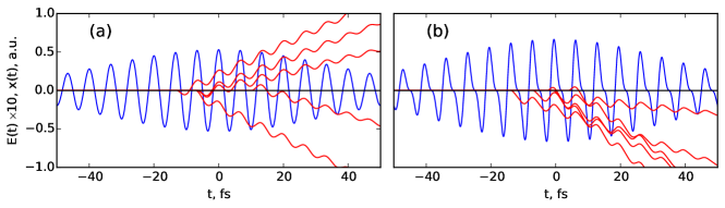
Figure 1: Trajectories $x(t)$ (red lines) of sample electrons ionized in the electric field $E(t)$ (blue line) of the strong one-color (a) and two-color (b) optical pulses (parameters are given in the text). In (b), because of presence of two colors, the field shape is slightly asymmetric which leads to an asymmetry between up- and down- directions in the electron trajectories and thus to significant change of the resulting macroscopic current $J(t)$ and thus the Brunel radiation $E_{Br}(t)$. This illustrates the importance of subcycle dynamics of the ionization and movement.

In Fig. 1 one can see an exemplary process of free electron creation and their dynamics for single- and two-color pump field. We consider the electric field $E(t)$ in the form:

$$E(t)=F_{1}(t)\cos{\omega_{0}t}+F_{2}(t)\cos{(2\omega_{0}t+\phi_{12}(t))},$$ (4)

where $\phi_{12}(t)$ is the phase which we allow to vary slowly in time, and

$$F_{i}(t)=\sqrt{2I_{i}(t)/(c\epsilon_{0})},\,\,I_{i}(t)=I_{i0}e^{-t^{2}/T_{i}^{2}},\,F_{0i}=\sqrt{2I_{0i}/(c\epsilon_{0})}.$$ (5)

are slowly varying field amplitudes and intensities which describe the corresponding pulse envelope, $T_{i}$ is the pulse duration, and $\phi_{12}$ is the relative phase.

In Fig. 1, several exemplary trajectories have been generated with the electron ionized randomly with the probability corresponding to the tunnel ionization rate as discussed below, for the cases of $I_{2}=0$ in Fig. 1(a) and $I_{2}=20$ TW/cm² in Fig. 1(b). In both cases we assumed $I_{1}=100$ TW/cm², the frequency $\omega_{0}$ corresponding to 2 $\mu$m wavelength, and pulse duration of 50 fs. For the parameters chosen here, the electrons are ionized with highest probability close to the maxima of electric field and by subsequent acceleration move, in average, away from the origin. Neither recollision no core potential were taken into account in our simulations. Remarkably, the net current in the case of a two-color field in Fig. 1(b) possesses a spatial asymmetry, which is absent in the single-color case. Therefore, the net current $J(t)$ is also very different in both cases. Already this simple example shows that the net current $J(t)$ and thus the Brunel radiation $E_{Br}$ can be significantly modified by the field dynamics on the subcycle scale.

Here we will show that the dynamics of ionization process itself can be also of critical importance for the macroscopic current buildup. As far as we know, there is no universally acceptable model which describes ionization dynamics for all intensities on all relevant timescales which is also valid for multicolor field. As it was mentioned before, for high intensities ($\gamma\ll 1$) the ionization takes place on the subcycle scale. In this case, the ionization rate depending on the instantaneous field strength, describing tunneling process in quasi-static approximation, is acceptable for arbitrary pulse shapes and thus arbitrary number of frequencies in the pulse. We use here the static tunneling approximation formula in the form Ammosov et al. (1986):

$$W_{ST}(t)=\frac{\alpha}{\tilde{E}(t)}\exp\left\{-\frac{\beta}{\tilde{E}(t)}\right\},$$ (6)

where $W_{ST}(t)$ is the ionization rate, $\tilde{E}(t)=|E(t)|/E_{a}$, $E_{a}\approx 5.14\times 10^{11}$ Vm^-1 is the field unit in atomic system of units (a.u.), coefficients $\alpha=4\omega_{a}r_{H}^{5/2}$ and $\beta=(2/3)r_{H}^{3/2}$ are defined through the ratio of ionization potentials of argon and hydrogen atoms $r_{H}=U_{Ar}/U_{H}$, $U_{H}=13.6$ eV, $U_{Ar}=15.6$ eV, and $\omega_{a}\approx 4.13\times 10^{16}$ s^-1.

For lower intensities $\gamma\gg 1$, when ionization probability is much less then an optical cycle, ionization rate depends more on the cycle-averaged intensity - that is, on the field envelope rather than instantaneous field strength. The tunnel ionization formula Eq. (6) does not catch this dynamics anymore. To calculate corresponding ionization rate for both single- and two-color fields we used the generalization of the well known Keldysh-Faisal-Reis theory Keldysh (1965); Faisal (1973); Reiss (1980) for the field with arbitrary number of harmonics, which was developed by Guo, Aberg and Crasemann Guo and Drake (1992) and which we abbreviate here as GAC model. In App. A the corresponding ionization rate for the case where the field contains two colors $\omega_{0}$, $2\omega_{0}$. This model provides us the dependence of the ionization rate on both intensities $I_{1}(t),I_{2}(t)$ and the relative phase $\phi_{12}$ in explicit (though cumbersome) formalism:

$$W_{GAC}(t)=W_{GAC}(I_{1}(t),I_{2}(t),\phi_{12}),$$ (7)

where $W_{GAC}$ is given by Eq. (36) and described in details in Appendix A. Importantly, now ionization does not depend on the instantaneous field but rather on the slow envelopes of the harmonics as well as on their phase $\phi_{12}$.

Finally, for the case of a single-color field there is a relatively simple formula derived by Ivanov and Yudin Yudin and Ivanov (2001), which correctly describes both cycle-averaged ionization rate and its slow and subcycle dynamics in both tunnel and multiphoton regimes. We will refer to this model as IY one, and the corresponding ionization rate is given by:

$$W_{IY}(t)=\alpha\exp{\left(-\beta^{\prime}F(t)^{2}-\beta^{\prime\prime}E(t)^{2}\right)},$$ (8)

where the field is assumed to be in the form Eq. (4) with $F_{2}=0$, thus $F(t)\equiv F_{1}(t)/E_{a}$ is the slow field envelope in Eq. (5) in the units of $E_{a}$, and the coefficients are defined as:

$$\alpha=\frac{\pi C_{k}^{2}}{\tau}\left(\frac{2\kappa^{3}}{F}\right)^{2Q/\kappa},\,\beta^{\prime}=\frac{2\sigma_{0}+\sigma_{0}^{\prime\prime}}{2\omega_{0}^{3}},\beta^{\prime\prime}=\frac{\sigma_{0}^{\prime\prime}}{2\omega_{0}^{3}},$$ (9)

$$\sigma_{0}=\frac{1}{2}(G^{2}-\frac{1}{2})\ln{C}-G\frac{\gamma}{2},\,$$ (10)

$$\sigma_{0}^{\prime\prime}=\ln{C}-2\frac{\gamma}{G},\,G=\sqrt{1+\gamma^{2}},\,C=2G^{2}-1+2G\gamma.$$ (11)

Here $\kappa=\sqrt{2r_{H}}$ ($r_{H}$ is defined below Eq. (6)), $\tau=\kappa/F$ is the tunneling time, $\gamma=\omega_{0}\tau$ is the Keldysh parameter, $Q$ is the effective charge of the ionic core ($Q=1$ for noble gases), $C_{k}$ is related to the radial asysmptote of the quantum orbital and in our case also $C_{k}\approx 1$. This formula is not applicable for multicolor fields, but for single-color ones it provides a possibility to inspect the transition between tunnel and multiphoton regime in details, which is done in the next section.

III Brunel harmonics in single-color fields

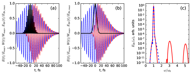
Figure 2: Brunel radiation in the tunnel and multiphoton regimes in the case of single color pulse. In (a) and (b), the field (blue line), ionization (black line) and $E_{Br}(t)$ (red line) are shown for $F_{01}=0.053$ a.u. (a) and $F_{01}=2.6\times 10^{-4}$ (200 times less) (b). The other parameters as in Fig. 1(a). In (c), the spectra of Brunel radiation $E_{Br}(\omega)$ for (a) (red line) and (b) (blue dashed line) are shown.

We start our consideration of Brunel radiation from discussing the single-color field ($I_{02}=0$) in Eq. (5), Eq. (4). We use Eq. (2) together with equation for the free electron density Eq. (3) and ionization calculated using IY formula $W=W_{IY}$ Eq. (8). In Fig. 2 the dynamics of the electric field and ionization as well as the Brunel radiation is shown for the parameters as in Fig. 1(a) but with two different intensities corresponding to the tunnel [Fig. 2(a)] and multiphoton [Fig. 2(b)] regime. Of course, the bare ionization rate $W$ in the case of the weak field is many orders of magnitude lower than in the tunnel one. We are interested in the dynamics, thus the ionization rate as well as Brunel radiation $E_{Br}(t)$ is renormalized to their maximum values in every case. The ionization rate in the tunnel regime demonstrates strong subcycle-scale dynamics whereas in the multiphoton regime it changes on much longer timescale of the slow field envelope. The Brunel radiation $E_{Br}(t)$ looks not very different in the time domain, but significant difference can be observed in the frequency range shown in Fig. 2(c). Namely, one can see that the Brunel harmonics at the frequencies $\omega=n\omega_{0}$, $n=3,5,7\ldots$ indeed arise if the ionization is in the tunnel regime (red lines) and disappears if multiphoton ionization takes place (blue lines). As it is shown in the next section, this is because the field of Brunel harmonics appears as a convolution of the fast optical field with the electron density, and this convolution has no new harmonics if the $\rho(t)$ changes slowly in time, as it is the case for the multiphoton regime. Note that the harmonic at $\omega=\omega_{0}$ is related related to the free electron movement (in contrast to electron birth) and is not interesting for us in the present article.

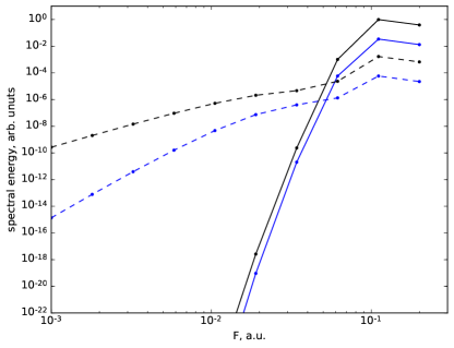
Figure 3: The energy of Brunel harmonics in dependence on the peak amplitude $F_{01}$ of a single-color pulse with the parameters as in Fig. 1(a). Black (blue) lines show the energy of the 3th (5th) harmonics. The absolute energies are shown in solid lines whereas the dashed lines represent the energies per single ionized atom.

Using IY formula it is possible to observe the transition between the two types of dynamics. Such transition is shown in Fig. 3, where the energies of the 3th and 5th Brunel harmonics are shown (solid black and blue lines, respectively) in dependence on the peak amplitude $F_{01}$ of the single-color field with the parameters as in Fig. 1(a). As the field amplitude decreases, the intensities of the Brunel harmonics decrease rather dramatically. There are two effects in this, one is connected to the overall density of free electrons, which also decreases, the other is connected to the ionization dynamics on its own. To demonstrate clearly the later effect, we plotted the energies rescaled per single ionized atom (technically, to obtain such quantities we rescale the ionization current $J$ and thus $E_{Br}$ to $\rho(t=\infty)/\rho_{0}$). The resulting quantities are shown in Fig. 3 by dashed lines.

If the Brunel harmonic energies depended only on the number of ionized electrons and not on the corresponding (subcycle) ionization dynamics, such rescaled energies would not depend on $F$. However, this is not the case.As one can see, they also decay quickly with decreasing $F$ (although with much lower rate), demonstrating the importance of the fast tunnel ionization dynamics. This decay is also much faster for the 5th harmonics than for the 3th one, indicating strong nonlinearity of the process. As it will be shown in Sec. 6,the appearance of 3th and 5th harmonics would be impossible if the ionization rate were truly slow (contains no harmonics at the pump frequency and higher). This shows also that the fast tunneling component in ionization dynamics is still present also for very low fields.

IV Brunel harmonics in two-color fields: commensurate case

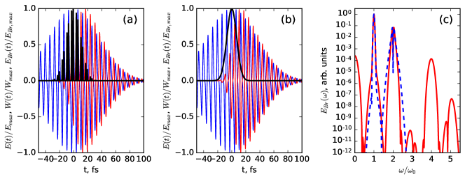
Figure 4: Brunel radiation in the tunnel and multiphoton regimes in the case of two-color pulse. In (a) and (b), the field (blue line), ionization (black line) and $E_{Br}(t)$ (red line) are shown for $F_{01}=0.053$ a.u. (a) and $F_{01}=2.6\times 10^{-4}$ a.u. (200 times less) (b). The other parameters as in Fig. 1(b). In (c), the spectra of Brunel radiation $E_{Br}(\omega)$ for (a) (red line) and (b) (blue dashed line) are shown.

Now let us return to the case when the pump pulse consists of the fundamental frequency $\omega_{0}$ and its second harmonics $2\omega_{0}$, that is, Eq. (4), Eq. (5) with $I_{02}\neq 0$, $\phi_{12}=\mathrm{const}$. In this case, both odd and even harmonics can appear. That is, Brunel harmonics are located near frequencies $\omega=n\omega_{0}$ with $n=0,2,3,4\ldots$. In particular, a zero one, which is located typically in realistic setups at THz frequency, is of special importance because THz radiation is difficult to generate. The appearance of even harmonics is related to the asymmetry of the field as shown in Fig. 1(b). For the two color case, as it was mentioned before, there is no general formula for ionization process allowing to track the transition from tunnel to multiphoton regime as we did this in Fig. 3. Nevertheless, we can consider these two cases separately, using tunnel ionization rate $W_{ST}$ (Eq. (6)) for higher intensities and GAC ionization rate $W_{GAC}$ for lower ones as discussed in Sec. II.

The corresponding figure for two-color case is presented in Fig. 4. The parameters are the same as in the single-color case in Fig. 2, but now $I_{02}\neq 0$, namely $I_{02}/I_{01}=0.2$ as in Fig. 1(b). In particular, we have taken $\phi_{12}=\pi/2$ which delivers the maximal energy for the THz harmonic Kim et al. (2007). One can see that the same behavior is observed: in the tunnel ionization regime the Brunel harmonics at $\omega=n\omega_{0}$ are visible whereas in the multiphoton regime they disappear. This behavior is completely analogous to the single-color case and takes place because in the multiphoton regime ionization is “too slow” to create harmonics as discussed further in Sec. 6.

V Brunel harmonics in two-color fields: incommensurate case

Let us now try two-color pump fields with incommensurate frequencies. By incommensurate frequencies we assume the ones with the ratio between them being not-integer. For this, we slightly detune the second harmonic $2\omega_{0}$ to $2\omega_{0}+\Delta\omega$ with $\Delta\omega\ll\omega_{0}$. That is, the electric field we consider is:

$$E(t)=\sqrt{2I_{1}(t)/(c\epsilon_{0})}\cos{\omega_{0}t}+\sqrt{2I_{2}(t)/(c\epsilon_{0})}\cos{(2\omega_{0}t+\Delta\omega t+\phi_{12})}.$$ (12)

The idea behind consideration of such field shape is the following: slight detuning $\Delta\omega\ll\omega_{0}$ leads in some slow beatings in the field amplitude, and in this case even “slow” ionization in multiphoton regime may “see” these beatings and thus generate some harmonics.

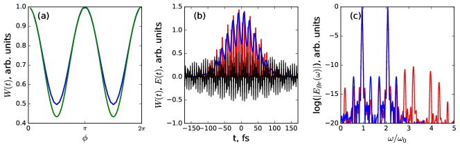
Figure 5: Brunel harmonics for incommensurate frequencies. (a) Two color multiphoton ionization rate $W_{GAC}(I_{1},I_{2},\phi)$ (normalized to the maximum over all $\phi$) depending on phases between two harmonics $\phi$ for $I_{1}=I_{2}=20$ TW/cm² (blue line) and $I_{1}=I_{2}=10$ TW/cm² (green line). (b) The field (black line), tunnel ionization rate (red line) and multiphoton ionization rate (blue line) for a 200 fs pulse containing frequencies $\omega_{0}$ and $2.2\omega_{0}$ with $I_{1}=I_{2}=20$ TW/cm². (c) Brunel harmonics (per single ionized electron) due to tunnel ionization (red line) and multiphoton ionization (blue line).

For the high intensity in the tunnel ionization regime we can still use the tunnel formula Eq. (6). On the other hand, the GAC formalism is valid for commensurate frequencies. However, we note that with the condition $\Delta\omega\ll\omega_{0}$, we can interpret the frequency shift as additional relative phase which is slowly varying in time:

$$\phi_{12}(t)\to\phi_{12}+\Delta\omega t$$ (13)

and thus consider the field in the form Eq. (4) with $\phi_{12}(t)$ given by Eq. (13). We then use the GAC formalism for two-color pump with frequencies $\omega_{0}$, $2\omega_{0}$ and the corresponding ionization rate

$$W(t)=W_{GAC}(I_{1}(t),I_{2}(t),\phi_{12}+\Delta\omega t),$$ (14)

with $W_{GAC}$ given in Eq. (36).

As one can see in Fig. 5(a), where the dependence of the multiphoton ionization rate on the phase between pulses for exemplary intensities $I_{1}$, $I_{2}$ is shown, the change of the effective phase effective phase $\Delta\omega t+\phi_{12}$ lead to noticeable modification of multiphoton ionization rate. Indeed, as one can see in the Fig. 5(b), not only tunnel ionization rate but also multiphoton one varies across the pulse. For this case we used longer pulses ($T_{1,2}=200$ fs) to make slow beatings possible, with the intensities $I_{1}=I_{2}=100$ TW/cm² for the tunnel case and $I_{1}=I_{2}=20$ TW/cm² for the multiphoton one.

The spectrum of the radiation generated by the Brunel mechanism for $\Delta\omega=0.2\omega_{0}$ is presented in Fig. 5(c). One can see the generation of new frequencies in the vicinity of the pump frequencies in the form of a comb-like pattern with spacing of roughly $0.4\Delta\omega$ both in the case of tunnel and multiphoton ionization regimes. This is in contrast to the pump pulse which have peaks only at $\omega_{0}$, $2\omega_{0}+3\Delta\omega$. In the multiphoton regime, only few such frequencies is generated [blue line in Fig. 5(c)]. Effectively, only frequencies $\omega_{0}\pm\Delta\omega$, $2\omega_{0}+\Delta\omega\pm 3\Delta\omega$ appear in this case. In contrast, in the tunnel ionization regime, this comb contains much more frequencies.

VI Analytical considerations of Brunel harmonics

To get a further insight into the processes governing the generation of new frequencies by Brunel mechanism, we present the quantities $E_{Br}(t)$, $E(t)$, and $\rho(t)$ as Fourier series near the maximum of the pump pulse. This method was first proposed in Brunel (1990) and further developed in Babushkin et al. (2011); de Alaiza Martínez et al. (2015); Balčiūnas et al. (2015). Here we neglect the slow amplitude changes due to Gaussian envelopes, that is, we consider pulses formally infinite in time to keep consideration simple. Under this condition, we have for the pump pulses with commensurate frequencies:

$$E_{Br}(t)=\sum_{n}E_{Br,n}e^{in\omega_{0}t},\,E(t)=\sum_{n}E_{n}e^{in\omega_{0}t},\,$$

$$\rho(t)=\sum_{n}\rho_{n}e^{in\omega_{0}t},W(t)=\sum_{n}W_{n}e^{in\omega_{0}t}.$$ (15)

If $\rho\ll\rho_{0}$ we can also assume $\partial_{t}\rho\approx\rho_{0}W$, that is:

$$\rho_{n}=\frac{\rho_{0}}{i\omega}W_{n}.$$ (16)

By substituting the series Eq. (VI) into Eq. (2), multiplicating the result by $e^{-in^{\prime}\omega_{0}t}$ and integrating over time (assuming that $\int_{-\infty}^{+\infty}e^{it\omega_{0}(n-n^{\prime})}dt=2\pi\delta_{n,n^{\prime}}$, where $\delta_{n,n^{\prime}}$ is the Kronecker delta), we get:

$$E_{Br,n}=\frac{ge^{2}}{m_{e}}\sum_{j}E_{j}\rho_{n-j}.$$ (17)

First, consider the situation arising when we are in multiphoton ionization regime. In this case, $\rho$ contains only the component $\rho_{0}$. That is,

$$\rho(t)=\rho_{0}.$$ (18)

In this case, the harmonics present in $E_{Br,n}$ coincide with the ones in the pump $E_{n}$:

$$E_{Br,n}=\frac{ge^{2}}{m_{e}}\rho_{0}E_{n},\,E_{Br}(t)=\sum_{n}E_{Br,n}e^{in\omega_{0}t}.$$ (19)

One can see that the slow dynamics of the electron density does not lead to generation of new harmonics, but rather to modification of the existing ones. This is valid for arbitrary pump spectra (with commensurate frequencies).

In contrast, in the case of tunneling ionization, $\rho(t)$ increases steeply each half optical period, and contains strong components with $n\neq 0$. In this case, the Brunel harmonics appear. In particular, if $E$ contains only a single frequency (that is, only $E_{1},E_{-1}\neq 0$), then from Eq. (17) we have:

$$E_{Br,n}=\frac{ge^{2}}{m_{e}}\left(E_{1}\sum_{j}\rho_{n-1}+E_{-1}\sum_{j}\rho_{n+1}\right).$$ (20)

In this case, only even components $\rho_{n}$, $n=2N$ are present, which results, according to Eq. (17), in appearance of odd harmonics in $E_{Br}(t)$. In contrast, for the two-color pump (we do not write the explicit formula for this case here), all components are present in $\rho_{n}$, and accordingly also in $E_{Br,n}$, including those with $n=0$.

In the case of non-commensurate frequencies, the series (VI) must be extended to include components with frequency $\Delta\omega$ and its multiples:

$$E_{Br}(t)=\sum_{n,m}E_{Br,n,m}e^{it(n\omega_{0}+m\Delta\omega)},\,E(t)=\sum_{n,m}E_{n,m}e^{it(n\omega_{0}+m\Delta\omega)},\,$$ (21)

$$\rho(t)=\sum_{n,m}\rho_{n,m}e^{it(n\omega_{0}+m\Delta\omega)},W(t)=\sum_{n,m}W_{n,m}e^{it(n\omega_{0}+m\Delta\omega)}.$$ (22)

Substituting into Eq. (2) and multiplying by $e^{-it(n^{\prime\prime}\omega_{0}+m^{\prime\prime}\Delta\omega)}$, we will have:

$$\sum_{n,m}E_{Br,n,m}e^{it(\omega_{0}(n-n^{\prime\prime})+\Delta\omega(m-m^{\prime\prime}))}=$$

$$=\sum_{n,m,n^{\prime},m^{\prime}}E_{n,m}\rho_{n^{\prime},m^{\prime}}e^{it(\omega_{0}(n+n^{\prime}-n^{\prime\prime})+\Delta\omega(m+m^{\prime}-m^{\prime\prime}))},$$ (23)

We can now integrate over time as we did by derivation of Eq. (17). In the case if there is no such $N$, $M$ that $N\omega_{0}+M\Delta\omega=0$ we can use the relation: $\int_{-\infty}^{+\infty}e^{it(\omega_{0}(n-n^{\prime\prime})+\Delta\omega(m-m^{\prime\prime}))}dt=2\pi\delta_{n,n^{\prime}}\delta_{m,m^{\prime\prime}}$, thus obtaining:

$$E_{Br,n,m}=\frac{ge^{2}}{m_{e}}\sum_{j,i}E_{j,i}\rho_{n-j,m-i}.$$ (24)

This equation is relatively good applicable in our situation since we need large $N$, $M$ to get $N\omega_{0}+M\Delta\omega=0$, which would require large number of harmonics in the spectrum.

In the multiphoton regime, because multiphoton ionization is fast enough to resolve beatings with frequency $\Delta\omega$ but still slow on the scale of fundamental frequency $\omega_{0}$, we have:

$$\rho(t)=\sum_{m}\rho_{0,m}e^{im\Delta\omega t},$$ (25)

which is to be compared to the multiphoton commensurate case Eq. (18). Because of this, instead of Eq. (19) we will have:

$$E_{Br,n,m}(\omega)=\frac{ge^{2}}{m_{e}}\sum_{j}\rho_{0,j}E_{n,m-j}.$$ (26)

As follows from the symmetry considerations and as one can see in Fig. 5, only even harmonics of $\Delta\omega$ occur in $W(t)$ and in $\rho$. This leads, according to Eq. (24), to generation of new frequencies $\omega_{0}+(2j+1)\Delta\omega$ and $2\omega_{0}+(2j+2)\Delta\omega$, $j=0,\pm 1,\pm 2,\ldots$, by Brunel mechanism, as shown in Fig. 5. In the tunnel non-commensurate case, the general formula Eq. (24) applies.

VII Discussion and conclusion

In conclusion, we have considered generation of the so-called Brunel harmonics in one- and two-color fields, comparing the situations when the ionization is fast subcycle tunneling process depending only on the instantaneous field (tunnel ionization regime valid for high fields), and the case when it has “memory” and depends on the cycle-average intensity (multiphoton regime valid for lower fields). We used approach of direct modeling of the classical net current produced by the ionized electrons and have shown that, at least in this classical approximation, in the multiphoton ionization the Brunel harmonics vanish in the multiphoton ionization regime. This shows that Brunel harmonics are very sensitive to the internal dynamics of the ionization process. For the single-color fields, we were able to show the transition between these two limits using Ivanov-Yudin approach which gives correctly both ionization rate and ionization dynamics. We confirmed that this behavior is also valid for two-color pump pulses containing a fundamental frequency and its second harmonics. Such pump pulses are especially interesting because they allow to generate THz frequencies, which are otherwise difficult to access by other optical methods. In this case, we considered only limiting cases of purely tunnel or purely multiphoton regime.

Nevertheless, for the two-color fields with the incommensurate frequencies ($\omega_{0}$ and $\omega_{0}+\Delta\omega$) and long enough pulses, the Brunel harmonics of the form $\omega_{0}+j\Delta\omega$ (for integer $j$) can arise also in multiphoton regime, because of the slow beatings between two harmonics on the time scale $\sim 1/\Delta\omega$. In general, by changing of this beat frequency, one can thus switch from “typical tunnel” to “typical multiphoton” regime, giving us a new tool to study the transition region between the two ionization regimes without changing the intensity which is an interesting direction for the future studies.

Funding

We gratefully acknowledge support by the DFG BA 4156/4-1, MO 850/20-1 and Nieders. Vorab ZN3061.

Appendix A Two-color multiphoton ionization

For description of multiphoton ionization we adopt here the Guo, Aberg and Crasemann (GAC) model Guo and Drake (1992), which is the generalization of the well known Keldysh-Faisal-Reis theory Keldysh (1965); Faisal (1973); Reiss (1980) for the field of sufficiently different frequencies and which was used in an optical setup Tzankov et al. (2007); Babushkin and Herrmann (2008). The GAC model is based on the scattering-matrix formalism, providing non-perturbative treatment of electron in electromagnetic field. In this section the units are used in which $\hbar=1$, $c=1$. It provides the cycle-average ionization rate for all intensities but fails to resolve the fast subcycle ionization rate dynamics in the tunnel ionization regime. In our case, we have two-color field (for instance $\omega+2\omega$) field. The Volkov state of the electron in bichromatic laser field with a quantized vector potential ${\mathrm{\mathbf{A}}}$:

$${\mathrm{\mathbf{A}}}(-{\mathrm{\mathbf{k}}}{\mathrm{\mathbf{r}}})=\sum_{j=1}^{2}g_{i}(\vec{\epsilon}_{j}e^{i{\mathrm{\mathbf{k}}}_{j}{\mathrm{\mathbf{r}}}}a_{j}+\vec{\epsilon}_{j}^{\;\ast}e^{i{\mathrm{\mathbf{k}}}_{j}{\mathrm{\mathbf{r}}}}a^{\dagger})$$ (27)

with polarization $\vec{\epsilon}_{j}=[\vec{\epsilon}_{x}\cos(\xi_{j}/2)+i\vec{\epsilon}_{y}\sin(\xi_{j}/2)]\exp(i\phi_{j})$, defined by ellipticity $\xi_{j}$ and phase $\phi_{j}$ for the modes $j=\omega,2\omega$, can be written as Guo and Drake (1992); Gao et al. (1998)

$$\left|\Psi_{\mu}\right>=V_{e}^{-1/2}\sum_{j_{1},j_{2}}\exp\{i[{\mathrm{\mathbf{P}}}_{e}+(u_{p1}-j_{1}){\mathrm{\mathbf{k}}}_{1}+(u_{p2}-j_{2}){\mathrm{\mathbf{k}}}_{2}]\}\mathcal{X}_{j_{1},j_{2}}(z)\left|n_{1}+j_{1},n_{2}+j_{2}\right>,$$ (28)

where $V_{e}$ is an integration volume, $n_{i}$ is a background photon number in the $i$th mode, $j_{i}$ is the number of transferred photons, ${\mathrm{\mathbf{P}}}_{e}$ us the momentum of the electron in the field, ${\mathrm{\mathbf{k}}}_{1}$, ${\mathrm{\mathbf{k}}}_{2}$ are the wavevectors of the corresponding field components, and $u_{p1}$, $u_{p2}$ are the ponderomotive parameters of the electron in the fields $\omega$ and $2\omega$ correspondingly:

$$u_{pi}=\frac{e^{2}\Lambda_{i}^{2}}{m_{e}\omega_{i}},$$ (29)

where $i=1,2$, $\omega_{1}=\omega$, $\omega_{2}=2\omega$, $2\Lambda_{i}$ is an amplitude of the $i$th mode, obtained from a quantized field Eq. (27) in the large photon limit $g_{i}\sqrt{n_{i}}\rightarrow\Lambda_{i}$.

$\mathcal{X}_{j_{1},j_{2}}(z)$ are the generalized phased Bessel functions (GPB) Gao et al. (1998); Zhang et al. (2004)

$$\mathcal{X}_{j_{1},j_{2}}(z)=\sum_{q_{1}\ldots q_{4}=-\infty}^{\infty}\left\{\mathrm{X}_{-j_{1}+2q_{1}+q_{3}+q_{4}}(\zeta_{1})X_{-j_{2}+2q_{2}+q_{3}-q_{4}}(\zeta_{2})\prod_{i=2}^{4}\mathrm{X}_{-q_{i}}(z_{i})\right\},$$ (30)

where $\mathrm{X}_{n}(z)=J_{n}(|z|)\exp\{in\arg(z)\}$ is a phased Bessel function Zhang et al. (2004), calculated through the usual Bessel function $J_{n}$ with arguments

$$\zeta_{i}=\frac{2|e|\Lambda_{i}}{m_{e}\omega_{i}}{\mathrm{\mathbf{P}}}\vec{\epsilon}_{i}, z_{i}=\frac{1}{2}u_{pi}\vec{\epsilon}_{i}\vec{\epsilon}_{i},\;\;\;\;(i=1,2)$$ (31)

$$z_{3}=\frac{2e^{2}\Lambda_{1}\Lambda_{2}\vec{\epsilon}_{1}{\mathrm{\mathbf{\epsilon}}}_{2}}{(\omega_{1}+\omega_{2})m_{e}}, z_{4}=\frac{2e^{2}\Lambda_{1}\Lambda_{2}\vec{\epsilon}_{1}{\mathrm{\mathbf{\epsilon}}}_{2}^{\ast}}{(\omega_{1}-\omega_{2})m_{e}}.$$ (32)

Using the interaction Hamiltonian of the electron and the quantized field ${\mathrm{\mathbf{A}}}$:

$$V({\mathrm{\mathbf{r}}})=\frac{-e}{2m_{e}}\left[(-i{\mathrm{\mathbf{\nabla}}}){\mathrm{\mathbf{A}}}+{\mathrm{\mathbf{A}}}(-i{\mathrm{\mathbf{\nabla}}})\right]+\frac{e^{2}{\mathrm{\mathbf{A}}}^{2}}{2m_{e}},$$ (33)

one can obtain the transition amplitude from the ground state inside an atom, described by a wavefunction $\Phi_{i}({\mathrm{\mathbf{r}}})$ and the energy $\mathcal{E}_{i}$, and $l_{1},\,l_{2}$ photons in the corresponding modes of the field, to an electron free state with a wavefunction $\phi_{f}({\mathrm{\mathbf{r}}})=e^{i{\mathrm{\mathbf{P}}}_{ef}{\mathrm{\mathbf{r}}}}$ and the energy $\mathcal{E}_{f}$, and $m_{1},\,m_{2}$ photons in the field Guo and Drake (1992).

$$T_{fi}=V_{e}^{-1/2}\sum_{\varepsilon_{\mu}=\varepsilon_{i}}\left<\phi_{f}({\mathrm{\mathbf{r}}});m_{1},m_{2}|\Psi_{\mu}\right>\left<\Psi_{\mu}|V({\mathrm{\mathbf{r}}})|\Phi_{i}({\mathrm{\mathbf{r}}});l_{1},l_{2}\right>=V_{e}^{-1/2}\mathcal{B}_{q_{1},q_{2}}^{(\omega_{1},\omega_{2})}({\mathrm{\mathbf{P}}}_{ef}),$$ (34)

where $q_{i}=l_{i}-m_{i}$, and $\mathcal{B}_{q_{1},q_{2}}^{(\omega_{1},\omega_{2})}({\mathrm{\mathbf{P}}}_{ef})$ is an (unnormalized) electron transition amplitude to the final state $\phi_{f}({\mathrm{\mathbf{r}}})$, accomplished by absorption of exactly $q_{i}$ photons from the $i$-th field mode:

$$\mathcal{B}_{q_{1},q_{2}}^{(\omega_{1},\omega_{2})}({\mathrm{\mathbf{P}}}_{ef})=\Phi_{i}({\mathrm{\mathbf{P}}}_{ef})\sum_{j_{1},j_{2}}\left[(u_{p1}-j_{1})\omega_{1}+(u_{p2}-j_{2})\omega_{2}\right]\mathcal{X}_{j_{1}-q_{1},j_{2}-q_{2}}(z_{f})\mathcal{X}^{\ast}_{j_{1},j_{2}}(z_{f}),$$ (35)

with $\Phi_{i}({\mathrm{\mathbf{P}}}_{ef})$ being a Fourier transform of $\Phi_{i}({\mathrm{\mathbf{r}}})$.

The total transition rate is then given by integration over all possible electron momenta and is expressed as a sum over the partial probabilities of absorption of particular number of “biphotons” $q=q_{1}+2q_{2}$ leading finally to:

$$W_{GAC}=\frac{V_{e}}{(2\pi)^{2}}\int\int d\Omega\>d|{\mathrm{\mathbf{P}}}_{ef}|\>\left\{|{\mathrm{\mathbf{P}}}_{ef}|^{2}\delta(\mathcal{E}_{i}-\mathcal{E}_{f})|T_{fi}|^{2}\right\}=$$

$$\frac{\sqrt{2m_{e}^{3}\omega}}{4\pi^{2}}\sum_{q}\sqrt{q-B/\omega}\int d\Omega\left|\sum_{q_{2}}\mathcal{B}_{q-2q_{2},q_{2}}^{(\omega,2\omega)}({\mathrm{\mathbf{p}}}_{ef})\right|^{2}.$$ (36)

Here, $B$ is an ionization potential, $\Omega$ is a solid angle ($d\Omega=\sin\theta_{{\mathrm{\mathbf{p}}}_{ef}}d\theta_{{\mathrm{\mathbf{p}}}_{ef}}d\phi_{{\mathrm{\mathbf{p}}}_{ef}}$), and ${\mathrm{\mathbf{p}}}_{ef}={\mathrm{\mathbf{n}}}_{\Omega}\sqrt{2m_{e}\omega(q-B/\omega)}$, ${\mathrm{\mathbf{n}}}_{\Omega}$ is a unit vector, pointing in the direction defined by the angle $\Omega$.

References

- Yudin and Ivanov (2001) G. L. Yudin and M. Y. Ivanov, Phys. Rev. A 64, 013409 (2001).
- Blaga et al. (2009) C. I. Blaga, F. Catoire, P. Colosimo, G. G. Paulus, H. G. Muller, P. Agostini, and L. F. DiMauro, Nat Phys 5, 335 (2009).
- Krausz and Ivanov (2009) F. Krausz and M. Ivanov, Rev. Mod. Phys. 81, 163 (2009).
- Torlina et al. (2015) L. Torlina, F. Morales, J. Kaushal, I. Ivanov, A. Kheifets, A. Zielinski, A. Scrinzi, H. G. Muller, S. Sukiasyan, M. Ivanov, and O. Smirnova, Nat Phys 11, 503 (2015), article.
- Shvetsov-Shilovski et al. (2016) N. I. Shvetsov-Shilovski, M. Lein, L. B. Madsen, E. Räsänen, C. Lemell, J. Burgdörfer, D. G. Arbó, and K. Tőkési, Phys. Rev. A 94, 013415 (2016).
- Ni et al. (2016) H. Ni, U. Saalmann, and J.-M. Rost, Phys. Rev. Lett. 117, 023002 (2016).
- Pisanty and Ivanov (2016) E. Pisanty and M. Ivanov, Phys. Rev. A 93, 043408 (2016).
- Jooya et al. (2016) H. Z. Jooya, D. A. Telnov, and S.-I. Chu, Phys. Rev. A 93, 063405 (2016).
- Shafir et al. (2013) D. Shafir, H. Soifer, C. Vozzi, A. S. Johnson, A. Hartung, Z. Dube, D. M. Villeneuve, P. B. Corkum, N. Dudovich, and A. Staudte, Phys. Rev. Lett. 111, 023005 (2013).
- Wu et al. (2012) C. Y. Wu, Y. D. Yang, Y. Q. Liu, Q. H. Gong, M. Wu, X. Liu, X. L. Hao, W. D. Li, X. T. He, and J. Chen, Phys. Rev. Lett. 109, 043001 (2012).
- Paulus et al. (1995) G. G. Paulus, W. Becker, and H. Walther, Phys. Rev. A 52, 4043 (1995).
- Reiss (2008) H. R. Reiss, Phys. Rev. Lett. 101, 043002 (2008).
- Topcu and Robicheaux (2012) T. Topcu and F. Robicheaux, Phys. Rev. A 86, 053407 (2012).
- Brunel (1990) F. Brunel, J. Opt. Soc. Am. B 7, 521 (1990).
- Balciunas et al. (2013) T. Balciunas, A. Verhoef, A. Mitrofanov, G. Fan, E. Serebryannikov, M. Ivanov, A. Zheltikov, and A. Baltuska, Chem. Phys. 414, 92 (2013).
- Cook and Hochstrasser (2000) D. J. Cook and R. M. Hochstrasser, Opt. Lett. 25, 1210 (2000).
- Kress et al. (2004) M. Kress, T. Löffler, S. Eden, M. Thomson, and H. G. Roskos, Opt. Lett. 29, 1120 (2004).
- Bartel et al. (2005) T. Bartel, P. Gaal, K. Reimann, M. Woerner, and T. Elsaesser, Opt. Lett. 30, 2805 (2005).
- Reimann (2007) K. Reimann, Rep. Progr. Phys. 70, 1597 (2007).
- Kim et al. (2008) K. Y. Kim, A. J. Taylor, J. H. Glownia, and G. Rodriguez, Nat Photon 2, 605 (2008).
- Babushkin et al. (2010) I. Babushkin, W. Kuehn, C. Köhler, S. Skupin, L. Bergé, K. Reimann, M. Woerner, J. Herrmann, and T. Elsaesser, Phys. Rev. Lett. 105, 053903 (2010).
- Babushkin et al. (2011) I. Babushkin, S. Skupin, A. Husakou, C. Köhler, E. Cabrera-Granado, L. Bergé, and J. Herrmann, New J. Phys. 13, 123029 (2011).
- Brée et al. (2011) C. Brée, A. Demircan, and G. Steinmeyer, Phys. Rev. Lett. 106, 183902 (2011).
- Wahlstrand et al. (2011) J. K. Wahlstrand, Y.-H. Cheng, Y.-H. Chen, and H. M. Milchberg, Phys. Rev. Lett. 107, 103901 (2011).
- Brown et al. (2012) J. M. Brown, E. M. Wright, J. V. Moloney, and M. Kolesik, Opt. Lett. 37, 1604 (2012).
- Béjot et al. (2010) P. Béjot, J. Kasparian, S. Henin, V. Loriot, T. Vieillard, E. Hertz, O. Faucher, B. Lavorel, and J.-P. Wolf, Phys. Rev. Lett. 104, 103903 (2010).
- Serebryannikov and Zheltikov (2014) E. E. Serebryannikov and A. M. Zheltikov, Phys. Rev. Lett. 113, 043901 (2014).
- Ammosov et al. (1986) M. V. Ammosov, N. B. Delone, and V. P. Krainov, Soviet Phys. JETP 64, 1191 (1986).
- Keldysh (1965) L. W. Keldysh, Sov. Phys. JETP 20 (1965).
- Faisal (1973) F. H. M. Faisal, J. Phys. B: Atom. Molec. Phys. 6, L89 (1973).
- Reiss (1980) H. R. Reiss, Phys. Rev. A 22, 1786 (1980).
- Guo and Drake (1992) D.-S. Guo and G. W. F. Drake, J. Phys. A: Math. Gen. 25, 5377 (1992).
- Kim et al. (2007) K.-Y. Kim, J. H. Glownia, A. J. Taylor, and G. Rodriguez, Opt. Express 15, 4577 (2007).
- de Alaiza Martínez et al. (2015) P. G. de Alaiza Martínez, I. Babushkin, L. Bergé, S. Skupin, E. Cabrera-Granado, C. Köhler, U. Morgner, A. Husakou, and J. Herrmann, Phys. Rev. Lett. 114, 183901 (2015).
- Balčiūnas et al. (2015) T. Balčiūnas, D. Lorenc, M. Ivanov, O. Smirnova, A. Zheltikov, D. Dietze, K. Unterrainer, T. Rathje, G. Paulus, A. Baltuška, et al., Opt. Express 23, 15278 (2015).
- Tzankov et al. (2007) P. Tzankov, O. Steinkellner, J. Zheng, M. Mero, W. Freyer, A. Husakou, I. Babushkin, J. Herrmann, and F. Noack, Opt. Express 15, 6389 (2007).
- Babushkin and Herrmann (2008) I. Babushkin and J. Herrmann, Opt. Express 16, 17774 (2008).
- Gao et al. (1998) L. Gao, X. Li, P. Fu, and D.-S. Guo, Phys. Rev. A 58, 3807 (1998).
- Zhang et al. (2004) J. Zhang, S. Li, and Z. Xu, Phys. Rev. A 69, 053410 (2004).