Geometrical contributions to the exchange constants: Free electrons with spin-orbit interaction

Abstract

Using thermal quantum field theory we derive an expression for the exchange constant that resembles Fukuyama’s formula for the orbital magnetic susceptibility (OMS). Guided by this formal analogy between the exchange constant and OMS we identify a contribution to the exchange constant that arises from the geometrical properties of the band structure in mixed phase space. We compute the exchange constants for free electrons and show that the geometrical contribution is generally important. Our formalism allows us to study the exchange constants in the presence of spin-orbit interaction (SOI). Thereby, we find sizable differences between the exchange constants of helical and cycloidal spin spirals. Furthermore, we discuss how to calculate the exchange constants based on a gauge-field approach in the case of the Rashba model with an additional exchange splitting and show that the exchange constants obtained from this gauge-field approach are in perfect agreement with those obtained from the quantum field theoretical method.

I Introduction

While the Berry phase has been shown to be important for spin-dynamics Niu and Kleinman (1998); Niu et al. (1999); Qian and Vignale (2002), less attention has been paid to geometrical aspects in the exchange constants. Recently, it has been shown that the Dzyaloshinskii-Moriya interaction (DMI), i.e., the asymmetric exchange, can be computed from a Berry phase approach, in which the geometrical properties of the electronic structure in mixed phase space play a key role Freimuth et al. (2014, 2013, 2016, 2016). DMI describes the linear change of the free energy with gradients in the magnetization direction. The effect of such noncollinear magnetic textures on conduction electrons can be accounted for by effective magnetic potentials Bruno et al. (2004); Fujita et al. (2011). Since orbital magnetism leads to a linear change of the free energy when an external magnetic field is applied, several formal analogies exist between the modern theory of orbital magnetization Resta (2010) and the Berry-phase approach to DMI Freimuth et al. (2014, 2016), because the latter captures the free energy change linear in an effective magnetic potential generated by the noncollinear magnetic texture.

Similarly, the (symmetric) exchange constants describe the quadratic change of the free energy with gradients in the magnetization direction while the orbital magnetic susceptibility (OMS) captures the quadratic change of the free energy with an applied magnetic field Fukuyama (1971). Therefore, it is natural to suspect formal analogies between the theories of OMS on the one hand and exchange constants on the other hand, which we will investigate in detail in this paper. For this purpose, we use thermal quantum field theory in order to express the exchange constants in terms of torque operators, velocity operators and the Green’s functions of a collinear ferromagnet and obtain a formula that resembles Fukuyama’s result for OMS Fukuyama (1971); Ogata and Fukuyama (2015).

Recently, geometrical contributions to OMS have been identified and shown to be generally significant and sometimes even dominant Gao et al. (2015); Piéchon et al. (2016). These contributions arise from the reciprocal-space Berry curvature and quantum metric, which describe geometrical properties of the electronic structure. We will show that, as a consequence of the formal analogies between OMS and exchange, similar geometrical contributions to the exchange constants can be identified, which arise from the Berry curvature and the quantum metric in mixed phase space as well as from the quantum metric in real space. In order to achieve this, we rewrite our Fukuyama-type formula for the exchange constant in terms of these geometrical properties.

Both the Fukuyama-type formula as well as the geometrical expression allow us to obtain the exchange constants directly from the electronic structure. Compared to the frozen spin-spiral approach Halilov et al. (1998); Kurz et al. (2004) such a formulation has the advantage that it becomes easier to investigate the relationship to spintronic and spincaloritronic effects. For example, the Berry phase theory of DMI allows us to relate DMI to the spin-orbit torque Freimuth et al. (2014), to ground-state spin-currents Freimuth et al. (2016), and to ground-state energy currents which need to be subtracted in order to extract the inverse thermal spin-orbit torque Freimuth et al. (2016). Similarly, torques due to the exchange interaction need to be considered in the theory of thermally induced spin-transfer torques Kohno et al. (2016), and a Green’s function expression of exchange is well suited for this purpose.

For the calculation of exchange constants in realistic materials powerful techniques exist already. Besides the frozen spin-spiral approach Halilov et al. (1998); Kurz et al. (2004); Şaşıoğlu et al. (2005); Ležaić et al. (2013) the method of infinitesimal rotations of magnetic moments and the Lichtenstein formula are popular Liechtenstein et al. (1987); Bergqvist et al. (2004); Ebert and Mankovsky (2009). In this work we focus on free electrons. However, the extension of the Fukuyama-type approach to calculations of exchange constants in realistic materials within the framework of first-principles density-functional theory has promising practical and technical perspectives. For example, a Fukuyama-type formula for the exchange constants might be an attractive alternative when spin-orbit interaction (SOI) is present, because in this case the frozen spin-spiral approach cannot be used and one needs to resort to supercell methods or use multiple scattering theory Ebert and Mankovsky (2009), which cannot be combined easily with all available density-functional theory codes. Similarly, for the first-principles simulation of the current-induced motion of domain walls and skyrmions, which involves complicated effects such as chiral damping Jué et al. (2015); Akosa et al. (2016) and the nonadiabatic torque Gilmore et al. (2011), and for the calculation of electronic transport properties – such as the topological Hall effect Franz et al. (2014) – in these noncollinear magnetic textures an approach that specifies the response to applied electric currents in terms of a coefficient matrix that is expanded in orders of the magnetization gradients is desirable. Since exchange constants are well-known for many materials, their calculation from a Fukuyama-type expression can be used for code-testing with the goal to extend the method to the mentioned spintronics effects.

This paper is structured as follows: In section II.1 we briefly review the derivation of Fukuyama’s formula for OMS, which serves as a basis to derive a Fukuyama-type expression for the exchange constants in section II.2. In section III.1 we discuss how to express OMS in terms of reciprocal-space curvatures and quantum metrices, which sets the stage to express the exchange constants in terms of mixed phase space curvatures and quantum metrices in section III.2. In section IV we show that – despite the spin-orbit interaction – the exchange constants can be obtained easily from a gauge-field approach in the case of the one-dimensional Rashba model. In section V.1 we discuss the exchange constants of the one-dimensional Rashba model. We show that the results obtained from the Fukuyama-type approach agree to those of the gauge-field approach, thereby demonstrating the validity of the Fukuyama-type expression even in the presence of SOI. Additionally, we discuss the geometrical contributions. In section V.2 we investigate the exchange constants in the two-dimensional Rashba model. This paper ends with a summary in section VI.

II Fukuyama method

II.1 Orbital magnetic susceptibility

The orbital magnetic susceptibility tensor ${\bm{\chi}}$ is defined by

$$\delta{\bm{M}}_{\rm orb}=\frac{1}{\mu_{0}}{\bm{\chi}}{\bm{B}},$$ (1)

where ${\bm{B}}$ is an applied external magnetic field and $\delta{\bm{M}}_{\rm orb}$ is the change of the orbital magnetization due to the application of ${\bm{B}}$. $\mu_{0}$ is the vacuum permeability. The $zz$ element of the orbital magnetic susceptibility tensor is given by the Fukuyama formula Fukuyama (1971)

$$\chi^{zz}=\frac{\mu_{0}e^{2}}{2\beta\hbar^{2}}\int\!\!\frac{{\rm d}^{d}k}{(2\pi)^{d}}\sum_{p}\text{Tr}\Bigl{[}$$ (2)

$$G^{\rm M}_{{\bm{k}}}(i\mathcal{E}_{p})v^{x}_{{\bm{k}}}G^{\rm M}_{{\bm{k}}}(i\mathcal{E}_{p})v^{y}_{{\bm{k}}}G^{\rm M}_{{\bm{k}}}(i\mathcal{E}_{p})v^{x}_{{\bm{k}}}G^{\rm M}_{{\bm{k}}}(i\mathcal{E}_{p})v^{y}_{{\bm{k}}}\Bigr{]},$$

where $d$ is the dimension ($d$=2 or $d$=3). In the case of twodimensional systems, such as a graphene sheet or a thin film, the $z$ direction is oriented perpendicular to the sheet or thin film. $v^{x}_{{\bm{k}}}$ and $v^{y}_{{\bm{k}}}$ are the $x$ and $y$ components of the velocity operator ${\bm{v}}_{{\bm{k}}}^{\phantom{k}}=e^{-i{\bm{k}}\cdot{\bm{r}}}{\bm{v}}e^{i{\bm{k}}\cdot{\bm{r}}}$ in crystal momentum representation, respectively. $\beta=(k_{\rm B}T)^{-1}$ is the inverse temperature, $k_{\rm B}$ is the Boltzmann constant, and $\mathcal{E}_{p}=\beta^{-1}(2p+1)\pi$ are the Matsubara points.

$$G^{\rm M}_{{\bm{k}}}(i\mathcal{E}_{p})=\hbar[i\mathcal{E}_{p}-H_{{\bm{k}}}]^{-1}$$ (3)

is the Matsubara Green’s function, where $H_{{\bm{k}}}$ is the Hamiltonian in crystal momentum representation.

Using the residue theorem the summation over Matsubara points can be replaced by an energy integration along the real energy axis as follows:

$$\chi^{zz}=-\frac{\mu_{0}e^{2}}{2\pi\hbar^{2}}\int\!\!\frac{{\rm d}^{d}k}{(2\pi)^{d}}{\rm Im}\int d\,\mathcal{E}\,f(\mathcal{E})\text{Tr}\Bigl{[}$$ (4)

$$G^{\rm R}_{{\bm{k}}}(\mathcal{E})v^{x}_{{\bm{k}}}G^{\rm R}_{{\bm{k}}}(\mathcal{E})v^{y}_{{\bm{k}}}G^{\rm R}_{{\bm{k}}}(\mathcal{E})v^{x}_{{\bm{k}}}G^{\rm R}_{{\bm{k}}}(\mathcal{E})v^{y}_{{\bm{k}}}\Bigr{]},$$

where $f(\mathcal{E})$ is the Fermi function and

$$G^{\rm R}_{{\bm{k}}}(\mathcal{E})=\hbar[\mathcal{E}-H_{{\bm{k}}}+i0^{+}]^{-1}$$ (5)

is the retarded Green’s function.

In the following we briefly sketch Fukuyama’s derivation Fukuyama (1971) of Eq. (2), which serves as a preparation for obtaining an expression for the exchange constants in section II.2. Since the vector potential of a homogeneous magnetic field is not compatible with Bloch boundary conditions we consider the spatially oscillating vector potential

$${\bm{A}}(x)=\frac{B_{0}}{q}\sin(qx)\hat{{\bm{e}}}_{y}$$ (6)

with corresponding magnetic field

$${\bm{B}}(x)=\nabla\times{\bm{A}}(x)=B_{0}\cos(qx)\hat{{\bm{e}}}_{z},$$ (7)

where $\hat{{\bm{e}}}_{y}$ and $\hat{{\bm{e}}}_{z}$ are unit vectors in the $y$ and $z$ directions, respectively. At the final stage of the calculation the limit $q\rightarrow 0$ will be taken. According to Eq. (1) this spatially oscillating magnetic field induces a spatially oscillating orbital magnetization. The interaction between this induced orbital magnetization and the magnetic field modifies the free energy density by the amount

$$\delta F =-\frac{1}{2}\langle\delta M_{\rm orb}^{z}B^{z}_{\phantom{z}}\rangle=-\frac{1}{2\mu_{0}}\chi^{zz}\langle B_{\phantom{z}}^{z}B^{z}_{\phantom{z}}\rangle=$$ (8)

$$=-\frac{1}{4\mu_{0}}\chi^{zz}[B_{0}]^{2},$$

where $\langle\dots\rangle$ denotes spatial averaging. The expression for $\chi^{zz}$ can be found by determining $\delta F$ from thermal quantum field theory and equating the result with Eq. (8).

The free energy is obtained from the partition function $\Xi$ as

$$F=-\frac{1}{\beta}\ln\Xi.$$ (9)

The modification of $\Xi$ due to the applied magnetic field ${\bm{B}}(x)$ is determined from perturbation theory. For example the contribution from second order perturbation theory is given by

$$\Xi^{(2)}= \frac{1}{2\hbar^{2}}\int_{0}^{\hbar\beta}\!\!\!\!d\tau_{1}\int_{0}^{\hbar\beta}\!\!\!\!d\tau_{2}\,\text{Tr}\left[e^{-\beta H}T_{\tau}\delta H_{\rm I}(\tau_{1})\delta H_{\rm I}(\tau_{2})\right]$$ (10)

$$= \frac{\Xi^{(0)}}{2\hbar^{2}}\int_{0}^{\hbar\beta}\!\!\!\!d\tau_{1}\int_{0}^{\hbar\beta}\!\!\!\!d\tau_{2}\,\langle T_{\tau}\delta H_{\rm I}(\tau_{1})\delta H_{\rm I}(\tau_{2})\rangle,$$

where $\Xi^{(0)}$ is the partition function of the unperturbed system, $T_{\tau}$ is the time-ordering operator, $H$ is the unperturbed Hamiltonian, and $\delta H_{\rm I}(\tau)=e^{\tau H/\hbar}\delta He^{-\tau H/\hbar}$ denotes the perturbation in the interaction picture.

Minimal coupling leads to two perturbation terms,

$$\delta H^{(1)}=\frac{e}{2}\left[{\bm{v}}\cdot{\bm{A}}(x)+{\bm{A}}(x)\cdot{\bm{v}}\right]$$ (11)

and

$$\delta H^{(2)} =\frac{e^{2}}{2m_{e}}{\bm{A}}^{2}(x)=\frac{e^{2}B_{0}^{2}}{2m_{e}q^{2}}\sin^{2}(qx)=$$ (12)

$$=\frac{e^{2}B_{0}^{2}}{4m_{e}q^{2}}[1-\cos(2qx)],$$

where $e>0$ is the elementary positive charge and $m_{e}$ is the electron mass. In order to determine $\chi^{zz}$ from Eq. (8) we need to find the modification of the free energy density $\delta F$ that arises from the perturbations $\delta H^{(1)}$ and $\delta H^{(2)}$ and that is second order in $B_{0}$. Thus, we need to perform second order perturbation theory with $\delta H^{(1)}$ and first order perturbation theory with $\delta H^{(2)}$.

In second quantization the perturbation $\delta H^{(1)}$ is given by

$$\delta H^{(1)} =\frac{eB_{0}}{4iq}\sum_{{\bm{k}}nm}\Bigl{\{}$$ (13)

$$\bigl{[}\langle u_{{\bm{k}}_{+}n}^{\phantom{y}}|v_{{\bm{k}}_{+}}^{y}|u_{{\bm{k}}_{-}m}^{\phantom{y}}\rangle+\langle u_{{\bm{k}}_{+}n}^{\phantom{y}}|v_{{\bm{k}}_{-}}^{y}|u_{{\bm{k}}_{-}m}^{\phantom{y}}\rangle\bigr{]}c^{\dagger}_{{\bm{k}}_{+}n}c^{\phantom{\dagger}}_{{\bm{k}}_{-}m}$$

$$- \bigl{[}\langle u_{{\bm{k}}_{-}n}^{\phantom{y}}|v_{{\bm{k}}_{-}}^{y}|u_{{\bm{k}}_{+}m}^{\phantom{y}}\rangle+\langle u_{{\bm{k}}_{-}n}^{\phantom{y}}|v_{{\bm{k}}_{+}}^{y}|u_{{\bm{k}}_{+}m}^{\phantom{y}}\rangle\bigr{]}c^{\dagger}_{{\bm{k}}_{-}n}c^{\phantom{\dagger}}_{{\bm{k}}_{+}m}\Bigr{\}},$$

where ${\bm{k}}_{+}={\bm{k}}+{\bm{q}}/2$ and ${\bm{k}}_{-}={\bm{k}}-{\bm{q}}/2$ and ${\bm{q}}=q\hat{{\bm{e}}}_{x}$. $|u_{{\bm{k}}n}\rangle$ denotes the eigenfunctions of the unperturbed Hamiltonian $H_{{\bm{k}}}$, such that $H_{{\bm{k}}}|u_{{\bm{k}}n}\rangle=\mathcal{E}_{{\bm{k}}n}|u_{{\bm{k}}n}\rangle$, where $\mathcal{E}_{{\bm{k}}n}$ is the band energy. $c^{\dagger}_{{\bm{k}}n}$ and $c^{\phantom{\dagger}}_{{\bm{k}}n}$ are creation and annihilation operators of an electron in band $n$ at $k$-point ${\bm{k}}$, respectively. Second order perturbation theory with respect to $\delta H^{(1)}$ modifies the free energy density by the amount

$$\delta F\!=\!\frac{e^{2}B^{2}_{0}}{4q^{2}\beta\hbar^{2}}\!\!\!\int\!\!\frac{{\rm d}^{d}k}{(2\pi)^{d}}\!\sum_{p}\!\text{Tr}\!\left[G^{\rm M}_{{\bm{k}}_{+}}(i\mathcal{E}_{p})v^{y}_{{\bm{k}}}G^{\rm M}_{{\bm{k}}_{-}}(i\mathcal{E}_{p})v^{y}_{{\bm{k}}}\right].$$ (14)

When the trace in Eq. (14) is Taylor-expanded in $q$ the zeroth-order term leads to a contribution to $\delta F$ that diverges like $q^{-2}$ in the limit $q\rightarrow 0$. This divergent term cancels out with the contribution from the piece $e^{2}B_{0}^{2}/(4m_{e}q^{2})$ in $\delta H^{(2)}$. The oscillating piece $-e^{2}B_{0}^{2}\cos(2qx)/(4m_{e}q^{2})$ in $\delta H^{(2)}$ averages out in first order perturbation theory. The $q$-quadratic term from the Taylor-expansion of the trace in Eq. (14) yields the free-energy change

$$\delta F\!=\!-\frac{e^{2}B_{0}^{2}}{8\beta\hbar^{2}}\!\!\!\int\!\!\frac{{\rm d}^{d}k}{(2\pi)^{d}}\!\sum_{p}\text{Tr}\left[\frac{\partial G^{\rm M}_{{\bm{k}}}(i\mathcal{E}_{p})}{\partial k^{x}_{\phantom{x}}}v^{y}_{{\bm{k}}}\frac{\partial G^{\rm M}_{{\bm{k}}}(i\mathcal{E}_{p})}{\partial k^{x}_{\phantom{x}}}v^{y}_{{\bm{k}}}\right].$$ (15)

With the help of Eq. (8) we obtain the susceptibility

$$\chi^{zz}\!=\!\frac{e^{2}\mu_{0}}{2\beta\hbar^{2}}\!\!\!\int\!\!\frac{{\rm d}^{d}k}{(2\pi)^{d}}\!\sum_{p}\text{Tr}\left[\frac{\partial G^{\rm M}_{{\bm{k}}}(i\mathcal{E}_{p})}{\partial k^{x}_{\phantom{x}}}v^{y}_{{\bm{k}}}\frac{\partial G^{\rm M}_{{\bm{k}}}(i\mathcal{E}_{p})}{\partial k^{x}_{\phantom{x}}}v^{y}_{{\bm{k}}}\right].$$ (16)

Employing the relation

$$\frac{\partial G^{\rm M}_{{\bm{k}}}(i\mathcal{E}_{p})}{\partial k^{x}}=G^{\rm M}_{{\bm{k}}}(i\mathcal{E}_{p})v^{x}_{{\bm{k}}}G^{\rm M}_{{\bm{k}}}(i\mathcal{E}_{p})$$ (17)

one finally obtains Eq. (2).

For completeness, we mention that it has been shown that Eq. (2) needs to be modified for the calculation of OMS from tight-binding models Raoux et al. (2015); Gómez-Santos and Stauber (2011). We do not discuss these modifications here.

II.2 Exchange constants

In order to derive an expression for the exchange constant we consider the case where the magnetization performs small sinusoidal oscillations around the $z$ direction as a function of the $x$ coordinate:

$$\hat{{\bm{n}}}(x)=\begin{pmatrix}\eta\sin(qx)\\ 0\\ 1\end{pmatrix}\frac{1}{\sqrt{1+\eta^{2}\sin^{2}(qx)}},$$ (18)

where $\hat{{\bm{n}}}(x)$ is a normalized vector that describes the magnetization direction and $\eta$ controls the amplitude of the oscillations. As a result of these oscillations the free energy density changes by the amount

$$\delta F=\mathscr{A}^{xx}\left\langle\left[\frac{\partial\hat{n}^{x}}{\partial x}\right]^{2}\right\rangle=\frac{1}{2}\eta^{2}q^{2}\mathscr{A}^{xx},$$ (19)

where $\mathscr{A}^{xx}$ is an exchange constant and where we neglected higher orders in $\eta$. In the presence of SOI the free energy change may depend on whether the magnetization oscillates in the $xz$ plane or in the $yz$ plane. When the magnetization oscillates in the $yz$ plane, i.e., when

$$\hat{{\bm{n}}}(x)=\begin{pmatrix}0\\ \eta\sin(qx)\\ 1\end{pmatrix}\frac{1}{\sqrt{1+\eta^{2}\sin^{2}(qx)}},$$ (20)

the corresponding free energy change is described by

$$\delta F=\mathscr{A}^{xy}\left\langle\left[\frac{\partial\hat{n}^{y}}{\partial x}\right]^{2}\right\rangle=\frac{1}{2}\eta^{2}q^{2}\mathscr{A}^{xy},$$ (21)

with the exchange constant $\mathscr{A}^{xy}$. $\mathscr{A}^{xy}$ may differ from $\mathscr{A}^{xx}$ in the presence of SOI. In the following we use thermal quantum field theory in order to obtain expressions for the free energy change $\delta F$ that arises from spatial oscillations of the magnetization direction as given by Eq. (18). We will then use Eq. (19) to obtain $\mathscr{A}^{xx}$. To simplify the notation we will focus on the component $\mathscr{A}^{xx}$. The generalization to the other exchange constants, such as $\mathscr{A}^{xy}$, is obvious.

We consider the Hamiltonian of a collinear ferromagnet with magnetization pointing in $z$ direction, given by

$$H({\bm{r}})= -\frac{\hbar^{2}}{2m_{e}}\Delta+V({\bm{r}})+\mu_{\rm B}^{\phantom{B}}\sigma^{z}\Omega^{\rm xc}({\bm{r}})+$$ (22)

$$+\frac{1}{2ec^{2}}\mu_{\rm B}^{\phantom{B}}{\bm{\sigma}}\cdot\left[{\bm{\nabla}}V({\bm{r}})\times{\bm{v}}\right].$$

The kinetic energy is described by the first term. The second term is a scalar potential. The third term describes the exchange interaction, where $\mu_{\rm B}^{\phantom{B}}$ is the Bohr magneton, ${\bm{\sigma}}=(\sigma^{x},\sigma^{y},\sigma^{z})^{\rm T}$ is the vector of Pauli spin matrices, and $\Omega^{\rm xc}({\bm{r}})$ is the exchange field. The last term is the spin-orbit interaction. When the magnetization direction is not collinear but spatially oscillating according to Eq. (18) the corresponding Hamiltonian is $H^{\prime}=H+\delta H^{(1)}+\delta H^{(2)}$ with

$$\delta H^{(1)}=\mu_{\rm B}^{\phantom{B}}\sigma^{x}\Omega^{\rm xc}({\bm{r}})\eta\sin(qx)=\mathcal{T}^{y}\eta\sin(qx)$$ (23)

and

$$\delta H^{(2)} =-\frac{1}{2}\mu_{\rm B}^{\phantom{B}}\sigma^{z}\Omega^{\rm xc}({\bm{r}})\eta^{2}\sin^{2}(qx)$$ (24)

$$=-\frac{1}{4}\mu_{\rm B}^{\phantom{B}}\sigma^{z}\Omega^{\rm xc}({\bm{r}})\eta^{2}\left[1-\cos(2qx)\right],$$

where ${\bm{\mathcal{T}}}=-\mu_{\rm B}^{\phantom{B}}{\bm{\sigma}}\times\hat{{\bm{e}}}^{z}\Omega^{\rm xc}$ is the torque operator and $\mathcal{T}^{y}$ is its $y$ component. According to Eq. (19) we need to find the modification of the free energy that is quadratic in $\eta$. Therefore, we need to perform second order perturbation theory with $\delta H^{(1)}$ and first order perturbation theory with $\delta H^{(2)}$.

The perturbation $\delta H^{(1)}$ can be written in second quantization in the form

$$\delta H^{(1)}=\frac{\eta}{2i}\sum_{{\bm{k}}nm}\Bigl{\{} \langle u_{{\bm{k}}_{+}n}^{\phantom{k}}|\mathcal{T}^{y}|u_{{\bm{k}}_{-}m}^{\phantom{k}}\rangle c^{\dagger}_{{\bm{k}}_{+}n}c^{\phantom{\dagger}}_{{\bm{k}}_{-}m}$$ (25)

$$- \langle u_{{\bm{k}}_{-}n}^{\phantom{k}}|\mathcal{T}^{y}|u_{{\bm{k}}_{+}m}^{\phantom{k}}\rangle c^{\dagger}_{{\bm{k}}_{-}n}c^{\phantom{\dagger}}_{{\bm{k}}_{+}m}\Bigr{\}}.$$

In second order perturbation theory with respect to $\delta H^{(1)}$ the free energy is modified by the amount

$$\delta F\!=\!\frac{\eta^{2}}{4\beta\hbar^{2}}\!\!\!\int\!\!\frac{{\rm d}^{d}k}{(2\pi)^{d}}\!\sum_{p}\!\text{Tr}\!\left[G^{\rm M}_{{\bm{k}}_{+}}(i\mathcal{E}_{p})\mathcal{T}^{y}G^{\rm M}_{{\bm{k}}_{-}}(i\mathcal{E}_{p})\mathcal{T}^{y}\right].$$ (26)

The zeroth-order term in the Taylor expansion of $\delta F$ with respect to $q$ cancels out with the contribution from the piece $-\frac{1}{4}\mu_{\rm B}^{\phantom{B}}\sigma^{z}\Omega^{\rm xc}({\bm{r}})\eta^{2}$ from $\delta H^{(2)}$ only when SOI is not included. This is an interesting difference to the case of the orbital magnetic susceptibility discussed below Eq. (14), where the corresponding cancellation happens always. This difference is due to the fact that the magnetic anisotropy energy gives rise to a contribution to $\delta F$ which in leading order is proportional to $\eta^{2}$ at the zeroth order in $q$. The oscillating piece $\frac{1}{4}\mu_{\rm B}^{\phantom{B}}\sigma^{z}\Omega^{\rm xc}({\bm{r}})\eta^{2}\cos(2qx)$ from $\delta H^{(2)}$ averages out in first order perturbation theory. In order to obtain the exchange constant $\mathscr{A}^{xx}$ we need the $q$-quadratic term from the Taylor-expansion of $\delta F$, which is given by

$$\delta F\!=\!-\frac{\eta^{2}q^{2}}{8\beta\hbar^{2}}\!\!\!\int\!\!\frac{{\rm d}^{d}k}{(2\pi)^{d}}\!\sum_{p}\!\text{Tr}\!\left[\frac{\partial G^{\rm M}_{{\bm{k}}_{+}}(i\mathcal{E}_{p})}{\partial k^{x}}\mathcal{T}^{y}\frac{\partial G^{\rm M}_{{\bm{k}}_{-}}(i\mathcal{E}_{p})}{\partial k^{x}}\mathcal{T}^{y}\right].$$ (27)

Using Eq. (17) and Eq. (19) we find the following expression for the exchange constant:

$$\mathscr{A}^{xx}=\frac{-1}{4\beta\hbar^{2}}\sum_{p}\int\!\!\frac{{\rm d}^{d}k}{(2\pi)^{d}}\text{Tr}\Bigl{[}$$ (28)

$$G^{\rm M}_{{\bm{k}}}(i\mathcal{E}_{p})\mathcal{T}^{y}G^{\rm M}_{{\bm{k}}}(i\mathcal{E}_{p})v^{x}_{{\bm{k}}}G^{\rm M}_{{\bm{k}}}(i\mathcal{E}_{p})\mathcal{T}^{y}G^{\rm M}_{{\bm{k}}}(i\mathcal{E}_{p})v^{x}_{{\bm{k}}}\Bigr{]},$$

which strongly resembles the Fukuyama formula for OMS, Eq. (2). Apart from the prefactor, Eq. (28) differs from Eq. (2) by the replacement of the velocity operator $v^{y}_{{\bm{k}}}$ by the torque operator $\mathcal{T}^{y}$.

The summation over Matsubara points can be expressed in terms of an energy integration along the real energy axis yielding

$$\mathscr{A}^{xx}=\frac{1}{4\pi\hbar^{2}}{\rm Im}\int d\,\mathcal{E}\,f(\mathcal{E})\int\!\!\frac{{\rm d}^{d}k}{(2\pi)^{d}}\text{Tr}\Bigl{[}$$ (29)

$$G^{\rm R}_{{\bm{k}}}(\mathcal{E})\mathcal{T}^{y}G^{\rm R}_{{\bm{k}}}(\mathcal{E})v^{x}_{{\bm{k}}}G^{\rm R}_{{\bm{k}}}(\mathcal{E})\mathcal{T}^{y}G^{\rm R}_{{\bm{k}}}(\mathcal{E})v^{x}_{{\bm{k}}}\Bigr{]}.$$

The unit of the exchange constant as given by Eq. (28) or Eq. (29) is energy times length when $d=1$ and it is energy when $d=2$ and it is energy per length when $d=3$. Consequently, the unit of the free energy density as given by Eq. (19) is energy per length when $d=1$ and it is energy per area when $d=2$ and it is energy per volume when $d=3$.

We have mentioned in the previous section that the Fukuyama formula for OMS needs to be modified for tight-binding models Raoux et al. (2015); Gómez-Santos and Stauber (2011). We expect similar modifications to be necessary when exchange constants are computed from tight-binding models, but we leave the discussion of these modifications for future work.

III Curvatures, quantum metrices, moments and polarizations

III.1 Orbital magnetic susceptibility

As discussed by Ogata et al. in Ogata and Fukuyama (2015) one can express the velocity operators and Green’s functions in Eq. (2) in the representation of Bloch eigenfunctions such that

$$\chi^{zz}=\frac{\mu_{0}e^{2}\hbar^{2}}{2\beta}\sum_{\begin{subarray}{c}nn^{\prime}\\ l\,l^{\prime}\end{subarray}}\int\!\!\frac{{\rm d}^{d}k}{(2\pi)^{d}}\Bigl{[}v^{x}_{{\bm{k}}nn^{\prime}}v^{y}_{{\bm{k}}n^{\prime}l}v^{x}_{{\bm{k}}ll^{\prime}}v^{y}_{{\bm{k}}l^{\prime}n}\Bigr{]}$$ (30)

$$\times\sum_{p}\frac{1}{i\mathcal{E}_{p}-\mathcal{E}_{{\bm{k}}n}}\frac{1}{i\mathcal{E}_{p}-\mathcal{E}_{{\bm{k}}n^{\prime}}}\frac{1}{i\mathcal{E}_{p}-\mathcal{E}_{{\bm{k}}l}}\frac{1}{i\mathcal{E}_{p}-\mathcal{E}_{{\bm{k}}l^{\prime}}},$$

where ${\bm{v}}^{\phantom{x}}_{{\bm{k}}nn^{\prime}}=\langle u_{{\bm{k}}n}|{\bm{v}}_{{\bm{k}}}^{\phantom{x}}|u_{{\bm{k}}n^{\prime}}\rangle$ denotes the matrix elements of the velocity operator, $\mathcal{E}_{{\bm{k}}n}$ is the energy of band $n$ at $k$-point ${\bm{k}}$ and $|u_{{\bm{k}}n}\rangle$ is the corresponding eigenstate of $H_{{\bm{k}}}$, i.e., $H_{{\bm{k}}}|u_{{\bm{k}}n}\rangle=\mathcal{E}_{{\bm{k}}n}|u_{{\bm{k}}n}\rangle$. The summations over Matsubara points can be carried out with the help of partial fraction decomposition and with the identity

$$\frac{1}{\beta}\sum_{p}\frac{1}{[i\mathcal{E}_{p}-\mathcal{E}_{{\bm{k}}n}]^{m}}=\frac{1}{(m-1)!}f_{{\bm{k}}n}^{(m-1)},$$ (31)

where $f_{{\bm{k}}n}^{(m-1)}$ is the $(m-1)$th derivative of the Fermi function. For example, when $n=n^{\prime}=l=l^{\prime}$ in Eq. (30) one uses Eq. (31) with $m=4$, which leads to a contribution with the third derivative of the Fermi function. In order to rewrite high derivatives of the Fermi function in terms of lower derivatives one employs integration by parts and the relation

$${\bm{v}}_{{\bm{k}}n}^{\phantom{x}}f^{(m+1)}_{{\bm{k}}n}=\frac{1}{\hbar}\frac{\partial f^{(m)}_{{\bm{k}}n}}{\partial{\bm{k}}},$$ (32)

where we defined ${\bm{v}}_{{\bm{k}}n}^{\phantom{x}}={\bm{v}}_{{\bm{k}}nn}^{\phantom{x}}$. Thereby one can achieve that only the first derivative of the Fermi function occurs. The resulting expression for the orbital magnetic susceptibility can be written as

$$\chi^{zz}= \mu_{0}\frac{e^{2}}{\hbar^{2}}\int\!\!\frac{{\rm d}^{d}k}{(2\pi)^{d}}\sum_{n}\Biggl{[}\frac{1}{12}f^{\prime}_{{\bm{k}}n}(\alpha^{xx}_{{\bm{k}}n}\alpha^{yy}_{{\bm{k}}n}-\alpha^{xy}_{{\bm{k}}n}\alpha^{yx}_{{\bm{k}}n})$$ (33)

$$- f^{\prime}_{{\bm{k}}n}m^{z}_{{\bm{k}}n}m^{z}_{{\bm{k}}n}-\frac{\hbar^{2}}{4m_{e}}f_{{\bm{k}}n}(g^{xx}_{{\bm{k}}n}+g^{yy}_{{\bm{k}}n})$$

$$+ \frac{3}{2}f_{{\bm{k}}n}\Omega^{z}_{{\bm{k}}n}m^{z}_{{\bm{k}}n}$$

$$+ \frac{1}{4}f_{{\bm{k}}n}(g^{xx}_{{\bm{k}}n}\alpha^{yy}_{{\bm{k}}n}+g^{yy}_{{\bm{k}}n}\alpha^{xx}_{{\bm{k}}n}-2g^{xy}_{{\bm{k}}n}\alpha^{yx}_{{\bm{k}}n})$$

$$+ \frac{\hbar^{2}}{2}f^{\prime}_{{\bm{k}}n}v^{x}_{{\bm{k}}n}\frac{\partial\langle u_{{\bm{k}}n}|}{\partial k^{y}}[v^{x}_{{\bm{k}}}+v^{x}_{{\bm{k}}n}]\frac{\partial|u_{{\bm{k}}n}\rangle}{\partial k^{y}}$$

$$+ \frac{\hbar^{2}}{2}f^{\prime}_{{\bm{k}}n}v^{y}_{{\bm{k}}n}\frac{\partial\langle u_{{\bm{k}}n}|}{\partial k^{x}}[v^{y}_{{\bm{k}}}+v^{y}_{{\bm{k}}n}]\frac{\partial|u_{{\bm{k}}n}\rangle}{\partial k^{x}}$$

$$- \frac{\hbar^{2}}{2}f^{\prime}_{{\bm{k}}n}v^{x}_{{\bm{k}}n}\frac{\partial\langle u_{{\bm{k}}n}|}{\partial k^{y}}[v^{y}_{{\bm{k}}}+v^{y}_{{\bm{k}}n}]\frac{\partial|u_{{\bm{k}}n}\rangle}{\partial k^{x}}$$

$$- \frac{\hbar^{2}}{2}f^{\prime}_{{\bm{k}}n}v^{y}_{{\bm{k}}n}\frac{\partial\langle u_{{\bm{k}}n}|}{\partial k^{x}}[v^{x}_{{\bm{k}}}+v^{x}_{{\bm{k}}n}]\frac{\partial|u_{{\bm{k}}n}\rangle}{\partial k^{y}}$$

$$- 2\hbar^{2}f_{{\bm{k}}n}\sum_{m\neq n}\frac{\mathcal{M}^{z}_{{\bm{k}}mn}\left[\mathcal{M}^{z}_{{\bm{k}}mn}\right]^{*}}{\mathcal{E}_{{\bm{k}}n}-\mathcal{E}_{{\bm{k}}m}}\Biggr{]},$$

where

$$\alpha^{ij}_{{\bm{k}}n}=\frac{\partial^{2}\mathcal{E}_{{\bm{k}}n}}{\partial k^{i}\partial k^{j}}$$ (34)

is the $ij$ element of the inverse effective mass tensor,

$$m^{z}_{{\bm{k}}n}=-{\rm Im}\left[\frac{\partial\langle u_{{\bm{k}}n}|}{\partial k^{x}}[\mathcal{E}_{{\bm{k}}n}-H]\frac{\partial|u_{{\bm{k}}n}\rangle}{\partial k^{y}}\right]$$ (35)

is the $z$ component of the orbital moment of the wavepacket associated with band $n$ at $k$-point ${\bm{k}}$ Sundaram and Niu (1999); Xiao et al. (2005),

$$g^{ij}_{{\bm{k}}n}={\rm Re}\left[\frac{\partial\langle u_{{\bm{k}}n}|}{\partial k^{i}}\Bigl{[}1-|u_{{\bm{k}}n}\rangle\langle u_{{\bm{k}}n}|\Bigr{]}\frac{\partial|u_{{\bm{k}}n}\rangle}{\partial k^{j}}\right]$$ (36)

is the $ij$ element of the ${\bm{k}}$-space quantum metrical tensor Anandan and Aharonov (1990); Neupert et al. (2013); Piéchon et al. (2016), $m_{e}$ is the electron mass,

$$\Omega^{z}_{{\bm{k}}n}=-2{\rm Im}\left[\frac{\partial\langle u_{{\bm{k}}n}|}{\partial k^{x}}\frac{\partial|u_{{\bm{k}}n}\rangle}{\partial k^{y}}\right]$$ (37)

is the ${\bm{k}}$-space Berry curvature, and

$${\bm{\mathcal{M}}}_{{\bm{k}}mn}=\frac{1}{2}\left[\sum_{n^{\prime}\neq n}{\bm{v}}_{{\bm{k}}mn^{\prime}}\times{\bm{A}}_{{\bm{k}}n^{\prime}n}+{\bm{v}}_{{\bm{k}}n}\times{\bm{A}}_{{\bm{k}}mn}\right]$$ (38)

are interband matrix elements of the magnetic dipole moment and of the position operator Gao et al. (2015), where

$${\bm{A}}_{{\bm{k}}mn}=i\langle u_{{\bm{k}}m}|\frac{\partial|u_{{\bm{k}}n}\rangle}{\partial{\bm{k}}}=i\hbar\frac{\langle u_{{\bm{k}}m}|{\bm{v}}|u_{{\bm{k}}n}\rangle}{\mathcal{E}_{{\bm{k}}n}-\mathcal{E}_{{\bm{k}}m}}$$ (39)

is the interband Berry connection.

A detailed discussion of all terms in Eq. (33) has been given by Gao et al. in Ref. Gao et al. (2015). In the semiclassical derivation of Gao et al. the terms in the lines 5, 6, 7 and 8 in Eq. (33) are explained by the $k$-space polarization energy and are related to the quadrupole moment of the velocity operator with respect to wave packets Gao et al. (2015). However, the semiclassical derivation yields a different prefactor for these polarization terms. Already Ogata et al. pointed out in Ref. Ogata and Fukuyama (2015) that the expression given by Gao et al. in Ref. Gao et al. (2015) differs from Eq. (2). However, Ogata et al. compared the semiclassical expression to the Fukuyama formula only in the special case of space-inversion symmetric systems when time-reversal symmetry is not broken. We find that Eq. (2) can generally be written in the form of Eq. (33), i.e., Eq. (33) yields the correct orbital magnetic susceptibility even in the time-reversal broken case and in systems lacking space inversion symmetry.

Only the last line in Eq. (33) involves interband couplings explicitly, while the first 8 lines in Eq. (33) are formulated in terms of single-band properties. The Berry curvature and the quantum metric describe the geometrical properties of a single-band. In this sense, lines 3 and 4 in Eq. (33) constitute the geometrical contribution to the orbital magnetic susceptibility Gao et al. (2015). In section III.2 we will identify analogous geometrical contributions to the exchange constants.

III.2 Exchange constants

As discussed in section III.1 the Fukuyama formula for the orbital magnetic susceptibility, Eq. (2), can be expressed in terms of geometrical properties such as the $k$-space Berry curvature and the quantum metric, and several other single-band properties, such as the orbital magnetic moment and the $k$-space polarization. The expression for the exchange constants, Eq. (28), has the same structure as Eq. (2) and can be obtained by replacing two velocity operators in Eq. (2) by torque operators. This formal similarity suggests that Eq. (28) can be expressed in terms of Berry curvatures and quantum metrices in mixed phase space. For this purpose we define the mixed Berry curvature Freimuth et al. (2013)

$$\mathcal{B}^{ij}_{{\bm{k}}n}=-2\,{\rm Im}\left\langle\frac{\partial u_{{\bm{k}}n}}{\partial\hat{n}^{i}}\left|\frac{\partial u_{{\bm{k}}n}}{\partial k^{j}}\right.\right\rangle,$$ (40)

where ${\bm{k}}$-derivatives are mixed with $\hat{{\bm{n}}}$-derivatives. Similarly, we define the mixed quantum metric

$$\mathcal{G}^{ij}_{{\bm{k}}n}={\rm Re}\left[\frac{\partial\langle u_{{\bm{k}}n}|}{\partial\hat{n}^{i}}\Bigl{[}1-|u_{{\bm{k}}n}\rangle\langle u_{{\bm{k}}n}|\Bigr{]}\frac{\partial|u_{{\bm{k}}n}\rangle}{\partial k^{j}}\right].$$ (41)

Additionally, we define the quantum metric in magnetization space

$$\tilde{g}^{ij}_{{\bm{k}}n}={\rm Re}\left[\frac{\partial\langle u_{{\bm{k}}n}|}{\partial\hat{n}^{i}}\Bigl{[}1-|u_{{\bm{k}}n}\rangle\langle u_{{\bm{k}}n}|\Bigr{]}\frac{\partial|u_{{\bm{k}}n}\rangle}{\partial\hat{n}^{j}}\right].$$ (42)

The twist-torque moment of wavepackets is described by Freimuth et al. (2014)

$$\mathcal{A}^{ij}_{{\bm{k}}n}=-{\rm Im}\left\langle\frac{\partial u_{{\bm{k}}n}}{\partial\hat{n}^{i}}\right|\!\Bigl{[}\mathcal{E}_{{\bm{k}}n}-H_{{\bm{k}}}\Bigr{]}\!\left|\frac{\partial u_{{\bm{k}}n}}{\partial k^{j}}\right\rangle,$$ (43)

and

$$\bar{A}^{j}_{{\bm{k}}mn}=i\langle u_{{\bm{k}}m}|\frac{\partial|u_{{\bm{k}}n}\rangle}{\partial\hat{n}^{j}}$$ (44)

is the interband Berry connection in magnetization space. The mixed phase-space analogue of the inverse effective mass tensor is given by

$$\bar{\alpha}^{ij}_{{\bm{k}}n}=\frac{\partial^{2}\mathcal{E}_{{\bm{k}}n}}{\partial k^{i}\partial\hat{n}^{j}}.$$ (45)

In Appendix A we explain how the derivatives with respect to magnetization direction are related to matrix elements of the torque operator.

In terms of the mixed phase-space quantities Eq. (40) through Eq. (45) the exchange constant can be written as

$$\mathscr{A}^{xx} =\int\!\!\frac{{\rm d}^{d}k}{(2\pi)^{d}}\sum_{n}\Biggl{[}\frac{1}{24}(f^{\prime\prime}_{{\bm{k}}n}\mathcal{T}^{y}_{{\bm{k}}n}\mathcal{T}^{y}_{{\bm{k}}n}\alpha^{xx}_{{\bm{k}}n}+f^{\prime}_{{\bm{k}}n}\bar{\alpha}^{xx}_{{\bm{k}}n}\bar{\alpha}^{xx}_{{\bm{k}}n})$$ (46)

$$+\frac{1}{2}f^{\prime}_{{\bm{k}}n}\mathcal{A}^{xx}_{{\bm{k}}n}\mathcal{A}^{xx}_{{\bm{k}}n}+\frac{1}{3}f_{{\bm{k}}n}\tilde{g}^{xx}_{{\bm{k}}n}\frac{\hbar^{2}}{m_{e}}$$

$$-\frac{5}{6}f_{{\bm{k}}n}\mathcal{A}^{xx}_{{\bm{k}}n}\mathcal{B}^{xx}_{{\bm{k}}n}$$

$$-\frac{1}{6}f_{{\bm{k}}n}\alpha^{xx}_{{\bm{k}}n}\tilde{g}^{xx}_{{\bm{k}}n}+\frac{1}{6}f_{{\bm{k}}n}\bar{\alpha}^{xx}_{{\bm{k}}n}\mathcal{G}^{xx}_{{\bm{k}}n}$$

$$+\mathscr{A}^{xx}_{\rm pol}+\mathscr{A}^{xx}_{\rm inter}\Biggr{]},$$

with

$$\mathscr{A}^{xx}_{\rm pol} =\int\!\!\frac{{\rm d}^{d}k}{(2\pi)^{d}}\sum_{n}\Biggl{[}$$ (47)

$$-\frac{1}{6}f^{\prime}_{{\bm{k}}n}\mathcal{T}^{y}_{{\bm{k}}n}\left\langle\frac{\partial u_{{\bm{k}}n}}{\partial k^{x}}\right|[\mathcal{T}^{y}_{\phantom{k}}+2\mathcal{T}^{y}_{{\bm{k}}n}]\left|\frac{\partial u_{{\bm{k}}n}}{\partial k^{x}}\right\rangle$$

$$-\frac{1}{6}\hbar^{2}f^{\prime}_{{\bm{k}}n}v^{x}_{{\bm{k}}n}\left\langle\frac{\partial u_{{\bm{k}}n}}{\partial\hat{n}^{x}}\right|[v^{x}_{{\bm{k}}}+v^{x}_{{\bm{k}}n}]\left|\frac{\partial u_{{\bm{k}}n}}{\partial\hat{n}^{x}}\right\rangle$$

$$+\frac{1}{3}\hbar f^{\prime}_{{\bm{k}}n}\mathcal{T}_{{\bm{k}}n}^{y}\left\langle\frac{\partial u_{{\bm{k}}n}}{\partial\hat{n}^{x}}\right|[2v^{x}_{{\bm{k}}}+v^{x}_{{\bm{k}}n}]\left|\frac{\partial u_{{\bm{k}}n}}{\partial k^{x}}\right\rangle\Biggr{]},$$

and

$$\mathscr{A}^{xx}_{\rm inter} =\int\!\!\frac{{\rm d}^{d}k}{(2\pi)^{d}}\sum_{n}\Biggl{[}\frac{\hbar^{2}}{3}f_{{\bm{k}}n}v^{x}_{{\bm{k}}n}v^{x}_{{\bm{k}}n}\sum_{m\neq n}\frac{\bar{A}^{x}_{{\bm{k}}mn}[\bar{A}^{x}_{{\bm{k}}mn}]^{*}}{\mathcal{E}_{{\bm{k}}n}-\mathcal{E}_{{\bm{k}}m}}$$ (48)

$$-\frac{2}{3}\hbar f_{{\bm{k}}n}v^{x}_{{\bm{k}}n}\mathcal{T}^{y}_{{\bm{k}}n}\sum_{m\neq n}\frac{\bar{A}^{x}_{{\bm{k}}mn}[A^{x}_{{\bm{k}}mn}]^{*}}{\mathcal{E}_{{\bm{k}}n}-\mathcal{E}_{{\bm{k}}m}}$$

$$-\frac{\hbar}{3}f_{{\bm{k}}n}\sum_{m\neq n}\frac{\sum\limits_{q\neq n}[v^{x}_{{\bm{k}}mq}\bar{A}^{x}_{{\bm{k}}qn}]^{*}\sum\limits_{r\neq n}\mathcal{T}^{y}_{{\bm{k}}mr}A^{x}_{{\bm{k}}rn}}{\mathcal{E}_{{\bm{k}}n}-\mathcal{E}_{{\bm{k}}m}}$$

$$+\frac{2}{3}\hbar^{2}f_{{\bm{k}}n}\sum_{m\neq n}\frac{\sum\limits_{q\neq n}[v^{x}_{{\bm{k}}mq}\bar{A}^{x}_{{\bm{k}}qn}]^{*}\sum\limits_{r\neq n}v^{x}_{{\bm{k}}mr}\bar{A}^{x}_{{\bm{k}}rn}}{\mathcal{E}_{{\bm{k}}n}-\mathcal{E}_{{\bm{k}}m}}$$

$$-\frac{1}{3}\hbar f_{{\bm{k}}n}v^{x}_{{\bm{k}}n}\sum_{m\neq n}\frac{[\bar{A}^{x}_{{\bm{k}}mn}]^{*}\sum\limits_{r\neq n}\mathcal{T}^{y}_{{\bm{k}}mr}A^{x}_{{\bm{k}}rn}}{\mathcal{E}_{{\bm{k}}n}-\mathcal{E}_{{\bm{k}}m}}$$

$$-\frac{2}{3}\hbar f_{{\bm{k}}n}\mathcal{T}^{y}_{{\bm{k}}n}\sum_{m\neq n}\frac{[A^{x}_{{\bm{k}}mn}]^{*}\sum\limits_{r\neq n}v^{x}_{{\bm{k}}mr}\bar{A}^{x}_{{\bm{k}}rn}}{\mathcal{E}_{{\bm{k}}n}-\mathcal{E}_{{\bm{k}}m}}$$

$$+f_{{\bm{k}}n}\mathcal{T}^{y}_{{\bm{k}}n}\sum_{m\neq n}\frac{[A^{x}_{{\bm{k}}mn}]^{*}\sum\limits_{r\neq n}\mathcal{T}^{y}_{{\bm{k}}mr}A^{x}_{{\bm{k}}rn}}{\mathcal{E}_{{\bm{k}}n}-\mathcal{E}_{{\bm{k}}m}}\Biggr{]},$$

where we defined $\mathcal{T}^{y}_{{\bm{k}}nn^{\prime}}=\langle u_{{\bm{k}}n}|\mathcal{T}^{y}_{\phantom{k}}|u_{{\bm{k}}n^{\prime}}\rangle$ and $\mathcal{T}^{y}_{{\bm{k}}n}=\mathcal{T}^{y}_{{\bm{k}}nn}$.

Eq. (46) differs substantially in structure from Eq. (33), while the corresponding Fukuyama-type expressions, Eq. (2) and Eq. (28), are very similar structurally. The structural differences between Eq. (46) and Eq. (33) arise, because there is no integration over the magnetization direction, only a Brillouin zone integration, and therefore the identity

$${\bm{\mathcal{T}}}_{{\bm{k}}n}^{\phantom{y}}f^{(m+1)}_{{\bm{k}}n}=\hat{{\bm{n}}}\times\frac{\partial f^{(m)}_{{\bm{k}}n}}{\partial\hat{{\bm{n}}}}$$ (49)

cannot be combined with integration by parts in order to rewrite high derivatives of the Fermi function in terms of lower derivatives of the Fermi function while Eq. (32) can be used for this purpose. For example, the first line in Eq. (46) is related formally to the Landau-Peierls susceptibility in the first line of Eq. (33): In the case of the orbital magnetic susceptibility the torque operators in the first line of Eq. (46) turn into velocity operators and one can use integration by parts such that

$$\int\!\!\frac{{\rm d}^{d}k}{(2\pi)^{d}}f^{\prime\prime}_{{\bm{k}}n}v^{y}_{{\bm{k}}n}v^{y}_{{\bm{k}}n}\alpha^{xx}_{{\bm{k}}n}=\int\!\!\frac{{\rm d}^{d}k}{(2\pi)^{d}}\frac{1}{\hbar}\frac{\partial f^{\prime}_{{\bm{k}}n}}{\partial k^{y}}v^{y}_{{\bm{k}}n}\alpha^{xx}_{{\bm{k}}n}=$$ (50)

$$- \int\!\!\frac{{\rm d}^{d}k}{(2\pi)^{d}}\frac{1}{\hbar}f^{\prime}_{{\bm{k}}n}\frac{\partial}{\partial k^{y}}[v^{y}_{{\bm{k}}n}\alpha^{xx}_{{\bm{k}}n}]=$$

$$- \int\!\!\frac{{\rm d}^{d}k}{(2\pi)^{d}}\frac{1}{\hbar}f^{\prime}_{{\bm{k}}n}[\alpha^{yy}_{{\bm{k}}n}\alpha^{xx}_{{\bm{k}}n}+v^{y}_{{\bm{k}}n}\frac{\partial}{\partial k^{y}}\alpha^{xx}_{{\bm{k}}n}],$$

which contains the term $f^{\prime}_{{\bm{k}}n}\alpha^{yy}_{{\bm{k}}n}\alpha^{xx}_{{\bm{k}}n}$ found also in the first line of Eq. (33).

The lines 2, 3 and 4 in Eq. (46) correspond to the lines 2, 3 and 4 in Eq. (33), where the twist torque moment $\mathcal{A}_{{\bm{k}}n}^{xx}$ replaces the orbital moment $m^{z}_{{\bm{k}}n}$, the $k$-space quantum metric $g_{{\bm{k}}n}^{yy}$ is replaced by the magnetization-space quantum metric $\tilde{g}_{{\bm{k}}n}^{xx}$, the mixed Berry curvature replaces the $k$-space Berry curvature, and the off-diagonal elements of the inverse effective mass, $\alpha_{{\bm{k}}n}^{yx}$, and of the $k$-space quantum metric, $g_{{\bm{k}}n}^{xy}$, are replaced by their mixed phase-space counterparts.

The contribution $\mathscr{A}_{\rm pol}^{xx}$ defined in Eq. (47) corresponds to the lines 5, 6, 7 and 8 in Eq. (33), which describe the $k$-space polarization energy. The contribution $\mathscr{A}_{\rm inter}^{xx}$ defined in Eq. (48) corresponds to the last line in Eq. (33) and is the only term that contains interband couplings explicitly.

Several terms in Eq. (46) are zero when SOI is not included in the Hamiltonian: The mixed phase-space analogue of the inverse effective mass, $\bar{\alpha}_{{\bm{k}}n}^{ij}$, is zero without SOI, because the band energy does not depend on the magnetization direction when SOI is absent. Additionally, $\mathcal{T}_{{\bm{k}}n}^{y}=0$, $\mathcal{A}^{ij}_{{\bm{k}}n}=0$, $\mathcal{B}^{ij}_{{\bm{k}}n}=0$ and $\mathcal{G}^{ij}_{{\bm{k}}n}=0$ in the absence of SOI. Thus, when SOI is absent the exchange constants are given by the considerably simpler expression

$$\mathscr{A}^{xx} =\int\!\!\frac{{\rm d}^{d}k}{(2\pi)^{d}}\sum_{n}\Biggl{[}\frac{1}{3}f_{{\bm{k}}n}\tilde{g}^{xx}_{{\bm{k}}n}\frac{\hbar^{2}}{m_{e}}$$ (51)

$$-\frac{1}{6}f_{{\bm{k}}n}\alpha^{xx}_{{\bm{k}}n}\tilde{g}^{xx}_{{\bm{k}}n}$$

$$-\frac{\hbar^{2}}{6}f^{\prime}_{{\bm{k}}n}v_{{\bm{k}}n}^{x}\left\langle\frac{\partial u_{{\bm{k}}n}}{\partial\hat{n}^{x}}\right|[v^{x}_{{\bm{k}}}+v^{x}_{{\bm{k}}n}]\left|\frac{\partial u_{{\bm{k}}n}}{\partial\hat{n}^{x}}\right\rangle$$

$$+\frac{\hbar^{2}}{3}f_{{\bm{k}}n}v^{x}_{{\bm{k}}n}v^{x}_{{\bm{k}}n}\sum_{m\neq n}\frac{\bar{A}^{x}_{{\bm{k}}mn}[\bar{A}^{x}_{{\bm{k}}mn}]^{*}}{\mathcal{E}_{{\bm{k}}n}-\mathcal{E}_{{\bm{k}}m}}$$

$$-\frac{\hbar}{3}f_{{\bm{k}}n}\sum_{m\neq n}\frac{\sum\limits_{q\neq n}[v^{x}_{{\bm{k}}mq}\bar{A}^{x}_{{\bm{k}}qn}]^{*}\sum\limits_{r\neq n}\mathcal{T}^{y}_{{\bm{k}}mr}A^{x}_{{\bm{k}}rn}}{\mathcal{E}_{{\bm{k}}n}-\mathcal{E}_{{\bm{k}}m}}$$

$$+\frac{2}{3}\hbar^{2}f_{{\bm{k}}n}\sum_{m\neq n}\frac{\sum\limits_{q\neq n}[v^{x}_{{\bm{k}}mq}\bar{A}^{x}_{{\bm{k}}qn}]^{*}\sum\limits_{r\neq n}v^{x}_{{\bm{k}}mr}\bar{A}^{x}_{{\bm{k}}rn}}{\mathcal{E}_{{\bm{k}}n}-\mathcal{E}_{{\bm{k}}m}}$$

$$-\frac{1}{3}\hbar f_{{\bm{k}}n}v^{x}_{{\bm{k}}n}\sum_{m\neq n}\frac{[\bar{A}^{x}_{{\bm{k}}mn}]^{*}\sum\limits_{r\neq n}\mathcal{T}^{y}_{{\bm{k}}mr}A^{x}_{{\bm{k}}rn}}{\mathcal{E}_{{\bm{k}}n}-\mathcal{E}_{{\bm{k}}m}}\Biggr{]}.$$

In Appendix B we discuss how to evaluate Eq. (51) analytically for simple model systems.

The lines 3 and 4 in Eq. (46) are the geometrical contribution to the exchange constants. It consists of three terms:

$$\mathscr{A}_{\rm geo1}^{xx}=-\frac{5}{6}\int\!\!\frac{{\rm d}^{d}k}{(2\pi)^{d}}\sum_{n}f_{{\bm{k}}n}\mathcal{A}^{xx}_{{\bm{k}}n}\mathcal{B}^{xx}_{{\bm{k}}n}$$ (52)

and

$$\mathscr{A}_{\rm geo2}^{xx}=-\frac{1}{6}\int\!\!\frac{{\rm d}^{d}k}{(2\pi)^{d}}\sum_{n}f_{{\bm{k}}n}\alpha^{xx}_{{\bm{k}}n}\tilde{g}^{xx}_{{\bm{k}}n}$$ (53)

and

$$\mathscr{A}_{\rm geo3}^{xx}=\frac{1}{6}\int\!\!\frac{{\rm d}^{d}k}{(2\pi)^{d}}\sum_{n}f_{{\bm{k}}n}\bar{\alpha}^{xx}_{{\bm{k}}n}\mathcal{G}^{xx}_{{\bm{k}}n}.$$ (54)

$\mathcal{B}^{xx}_{{\bm{k}}n}$ and $\mathcal{G}^{xx}_{{\bm{k}}n}$ describe geometrical properties of the bands in mixed phase space. When SOI is not included in the Hamiltonian $\mathscr{A}_{\rm geo1}^{xx}$ and $\mathscr{A}_{\rm geo3}^{xx}$ are zero. $\mathscr{A}_{\rm geo2}^{xx}$ is nonzero even in the absence of SOI. It involves $\tilde{g}^{xx}_{{\bm{k}}n}$, which describes the geometrical properties of the bands in real space.

According to Eq. (47) $\mathscr{A}^{xx}_{\rm pol}$ contains only terms with $f^{\prime}_{{\bm{k}}n}$. The derivative of the Fermi function becomes large close to the Fermi energy. In particular at zero temperature we have $f^{\prime}_{{\bm{k}}n}=-\delta(\mathcal{E}_{\rm F}-\mathcal{E}_{{\bm{k}}n})$. Therefore only states close to the Fermi level contribute to $\mathscr{A}^{xx}_{\rm pol}$, i.e., $\mathscr{A}^{xx}_{\rm pol}$ is a Fermi surface term. In contrast, $\mathscr{A}^{xx}_{\rm inter}$ (Eq. (48)) contains only terms with $f_{{\bm{k}}n}$, i.e., all states below the Fermi energy contribute to $\mathscr{A}^{xx}_{\rm inter}$. Hence, $\mathscr{A}^{xx}_{\rm inter}$ is a Fermi sea term. Eq. (46) contains additional Fermi surface and Fermi sea terms. The exchange constant in magnetic band insulators arises from the Fermi sea terms, since the Fermi surface terms are zero in insulators.

IV Gauge-field approach

The appearance of gauge-fields and their application in spintronics has been discussed in detail in the review Ref. Fujita et al. (2011). They can occur in real-space, momentum-space and in time. Here, we are interested in the Berry gauge field associated with electron spins that adiabatically follow noncollinear magnetic textures. This gauge field mimics the magnetic vector potential known from electrodynamics. The curl of this effective magnetic vector potential has similar consequences like a real magnetic field. In particular it deflects electrons by an effective Lorentz force, which leads to the topological Hall effect Bruno et al. (2004). The curl of the effective magnetic vector potential is nonzero when the scalar spin chirality of the magnetic texture is nonzero, for example in skyrmions. For the discussion of the exchange constants it is not necessary to consider systems with nonzero scalar spin chirality. But even when the curl of the effective magnetic vector potential is zero it does have consequences, in particular it affects the energy of the eigenstates, as we will see below.

In the case of the topological Hall effect the gauge-field approach has been developed for systems without SOI Bruno et al. (2004). In the general case it is difficult to apply the gauge-field approach to magnetic systems with SOI. However, under certain conditions the exchange constants can be obtained from a gauge-field approach even in the presence of SOI. We demonstrate this in the following. We will show that the exchange constants calculated based on the gauge-field approach agree to those given by Eq. (28). This will prove the accuracy of Eq. (28).

We consider the Rashba model with an additional exchange splitting (see Ref. Manchon et al. (2015) for a recent review on the Rashba model)

$$H=\frac{-\hbar^{2}}{2m_{e}}\Delta-i\alpha({\bm{\nabla}}\times\hat{{\bm{e}}}_{z})\cdot{\bm{\sigma}}+\frac{\Delta V}{2}{\bm{\sigma}}\cdot\hat{{\bm{n}}}_{\rm c}({\bm{r}}),$$ (55)

where the first, second and third terms on the right-hand side describe the kinetic energy, the Rashba spin-orbit coupling and the exchange interaction, respectively. We focus on the case of a flat cycloidal spin-spiral, where the magnetization direction $\hat{{\bm{n}}}_{\rm c}({\bm{r}})$ is given by

$$\hat{{\bm{n}}}_{\rm c}({\bm{r}})=\begin{pmatrix}\sin(qx)\\ 0\\ \cos(qx)\end{pmatrix}.$$ (56)

The exchange interaction describing the noncollinear spin-spiral in Eq. (55) can be transformed into an effective exchange interaction of a collinear magnet with the help of the unitary transformation

$$U(x)=\left(\begin{array}[]{cc}\cos(\frac{qx}{2})&-\sin(\frac{qx}{2})\\[6.0pt] \sin(\frac{qx}{2})&\cos(\frac{qx}{2})\end{array}\right)$$ (57)

such that Bruno et al. (2004)

$$U^{\dagger}(x)\frac{\Delta V}{2}{\bm{\sigma}}\cdot\hat{{\bm{n}}}_{\rm c}({\bm{r}})U(x)=\frac{\Delta V}{2}\sigma_{z}.$$ (58)

The kinetic energy in Eq. (55) transforms under this unitary transformation as follows Bruno et al. (2004):

$$-\frac{\hbar^{2}}{2m_{e}}U^{\dagger}\Delta U=$$ (59)

$$=-\frac{\hbar^{2}}{2m_{e}}U^{\dagger}\frac{\partial}{\partial{\bm{r}}}\cdot\left(U\frac{\partial}{\partial{\bm{r}}}+\frac{\partial U}{\partial{\bm{r}}}\right)$$

$$=-\frac{\hbar^{2}}{2m_{e}}\left(\Delta+2U^{\dagger}\frac{\partial U}{\partial x}\frac{\partial}{\partial x}+U^{\dagger}\frac{\partial^{2}U}{\partial x^{2}}\right).$$

The derivatives of $U$ with respect to the $x$ coordinate are

$$\frac{\partial U(x)}{\partial x}=\frac{q}{2}\left(\begin{array}[]{cc}-\sin(\frac{qx}{2})&-\cos(\frac{qx}{2})\\[6.0pt] \cos(\frac{qx}{2})&-\sin(\frac{qx}{2})\end{array}\right)$$ (60)

and

$$\frac{\partial^{2}U(x)}{\partial x^{2}}=-\frac{q^{2}}{4}U(x)$$ (61)

and we have

$$[U(x)]^{\dagger}\frac{\partial U(x)}{\partial x}=\frac{q}{2}\left(\begin{array}[]{cc}0&-1\\ 1&0\end{array}\right)=\frac{q}{2i}\sigma_{y}$$ (62)

such that the kinetic energy transforms as

$$-\frac{\hbar^{2}}{2m_{e}}U^{\dagger}\Delta U=-\frac{\hbar^{2}}{2m_{e}}\left(\Delta-iq\sigma_{y}\frac{\partial}{\partial x}-\frac{q^{2}}{4}\right).\\$$ (63)

Next, we need to find out how the Rashba SOI

$$\frac{1}{i}\alpha{\bm{\sigma}}\cdot({\bm{\nabla}}\times\hat{{\bm{e}}}_{z})=\frac{1}{i}\alpha\left[\sigma_{x}\frac{\partial}{\partial y}-\sigma_{y}\frac{\partial}{\partial x}\right]$$ (64)

transforms under $U$. We have

$${}^{\dagger}\sigma_{y}\frac{\partial U(x)}{\partial x}=-i\frac{q}{2}$$ (65)

and

$${}^{\dagger}\sigma_{y}U(x)=\sigma_{y}$$ (66)

and thus

$$-[U(x)]^{\dagger}\left[\frac{\alpha}{i}\sigma_{y}\frac{\partial}{\partial x}\right]U(x)=$$ (67)

$$= -[U(x)]^{\dagger}\left[\alpha\sigma_{y}\right]U(x)\frac{1}{i}\frac{\partial}{\partial x}$$

$$-[U(x)]^{\dagger}\left[\frac{\alpha}{i}\sigma_{y}\right]\frac{\partial U(x)}{\partial x}=$$

$$= -\alpha\sigma_{y}\frac{1}{i}\frac{\partial}{\partial x}+\frac{\alpha q}{2}.$$

However

$$[U(x)]^{\dagger}\sigma_{x}U(x)=$$ (68)

$$=\left(\begin{matrix}2\cos^{2}(\frac{qx}{2})-1&-2\cos(\frac{qx}{2})\sin(\frac{qx}{2})\\[6.0pt] -2\cos(\frac{qx}{2})\sin(\frac{qx}{2})&-2\cos^{2}(\frac{qx}{2})+1\end{matrix}\right)$$

depends on the $x$ coordinate and consequently the application of the $U$ transformation to Eq. (55) transforms the $x$-dependence of the exchange interaction into an $x$-dependence of SOI and no simplification is achieved by this transformation.

Therefore, we consider now the one-dimensional version of the Rashba model with an additional exchange splitting

$$H=\frac{-\hbar^{2}}{2m_{e}}\frac{\partial^{2}}{\partial x^{2}}+i\alpha\sigma_{y}\frac{\partial}{\partial x}+\frac{\Delta V}{2}{\bm{\sigma}}\cdot\hat{{\bm{n}}}_{\rm c}({\bm{r}}).$$ (69)

The one-dimensional Rashba model can be used to describe spin-split bands in one-dimensional atomic chains on surfaces Barke et al. (2006). Application of the $U$ transformation to Eq. (69) yields

$$\tilde{H}=[U(x)]^{\dagger}HU(x) =-\frac{\hbar^{2}}{2m_{e}}\left[\frac{\partial^{2}}{\partial x^{2}}-iq\sigma_{y}\frac{\partial}{\partial x}-\frac{q^{2}}{4}\right]+$$ (70)

$$+\frac{\Delta V}{2}\sigma_{z}-\alpha\sigma_{y}\frac{1}{i}\frac{\partial}{\partial x}+\frac{\alpha q}{2}$$

and the corresponding crystal-field representation of the Hamiltonian is given by

$$\tilde{H}_{k_{x}} =\frac{\hbar^{2}}{2m_{e}}\left[k_{x}^{2}-qk_{x}\sigma_{y}+\frac{q^{2}}{4}\right]+$$ (71)

$$+\frac{\Delta V}{2}\sigma_{z}-\alpha k_{x}\sigma_{y}+\frac{\alpha q}{2}.$$

Since the $U$ transformation preserves the eigenvalues, the Hamiltonian $\tilde{H}_{k_{x}}$ has the same spectrum as Eq. (69). However, $\tilde{H}_{k_{x}}$ is position-independent and thus it is straightforward to determine its eigenvalues, while the original Hamiltonian in Eq. (69) is more difficult to deal with due to the position-dependence of the exchange term for the cycloidal spin-spiral.

The reason why the $U$ transformation can be used to simplify Eq. (69) into $\tilde{H}_{k_{x}}$ lies in the spin-rotation symmetry of Eq. (69): The Hamiltonian is invariant under the simultaneous rotation of the spin-operator and the magnetization direction $\hat{{\bm{n}}}_{c}$ around the $y$ axis. In contrast, the Hamiltonian of the two-dimensional Rashba model, Eq. (55), does not exhibit this symmetry when $\alpha\neq 0$.

The Hamiltonian Eq. (70) can be rewritten in the form

$$H=\frac{1}{2m}(p_{x}+eA^{\rm eff})^{2}-\frac{m\alpha^{2}}{2\hbar^{2}}$$ (72)

where $p_{x}=-i\hbar\partial/\partial x$ is the $x$ component of the momentum operator and

$$A^{\rm eff}=-\frac{m}{e\hbar}\left(\alpha+\frac{\hbar^{2}}{2m}q\right)\sigma_{y}$$ (73)

can be considered as an effective magnetic vector potential, which is why we refer to this method as gauge-field approach.

The free energy density $F_{q}$ of the one-dimensional Rashba model with exchange splitting, Eq. (69), can be obtained from

$$F_{q}=-\frac{1}{\beta}\int\frac{d\,k_{x}}{2\pi}\sum_{n}\ln\left[1+e^{-\beta(\mathcal{E}_{k_{x},q,n}-\mu)}\right],$$ (74)

where $\mathcal{E}_{k_{x},q,n}$ denotes the $n$th eigenvalue of $\tilde{H}_{k_{x}}$ at $k$-point $k_{x}$ and spin-spiral wavenumber $q$. Equating $F_{q}$ and the phenomenological expression for the free energy

$$F_{q}=F_{0}+D^{yx}q+\mathscr{A}^{xx}q^{2}$$ (75)

allows us to determine the DMI-coefficient and the exchange parameter as follows:

$$D^{yx}=\frac{F_{q}-F_{-q}}{2q}$$ (76)

and

$$\mathscr{A}^{xx}=\frac{F_{q}+F_{-q}-2F_{0}}{2q^{2}}.$$ (77)

In section V.1 we will compare the exchange constant $\mathscr{A}^{xx}$ obtained from Eq. (77) to the one given by Eq. (28) and find perfect agreement between these two rather different approaches. Additionally, we will show in section V.1 that the DMI-coefficient $D^{yx}$ obtained from Eq. (76) is in perfect agreement with the one given by the Berry-phase theory of DMI Freimuth et al. (2014, 2013, 2016, 2016), which in the one-dimensional case runs

$$D^{yx}\!\!=\!\!\int\!\frac{d\,k_{x}}{2\pi}\!\sum_{n}\Bigl{[}f_{{\bm{k}}n}\mathcal{A}_{{\bm{k}}n}^{xx}\!+\!\frac{1}{\beta}\ln\left[1+e^{-\beta(\mathcal{E}_{{\bm{k}}n}-\mu)}\right]\mathcal{B}_{{\bm{k}}n}^{xx}\Bigr{]}.$$ (78)

IV.1 Two-dimensional electron gas without SOI

Due to Eq. (68) the $U$ transformation does not lead to simplifications in the case of the two-dimensional Rashba model Eq. (55) when $\alpha\neq 0$. However, in the case of $\alpha=0$ the $U$ transformation leads to a simplification of Eq. (55):

$$\tilde{H}= [U(x)]^{\dagger}HU(x)=$$ (79)

$$= -\frac{\hbar^{2}}{2m_{e}}\left[\Delta-iq\sigma_{y}\frac{\partial}{\partial x}-\frac{q^{2}}{4}\right]+\frac{\Delta V}{2}\sigma_{z},$$

with corresponding crystal momentum representation

$$\tilde{H}_{{\bm{k}}}=\frac{\hbar^{2}}{2m_{e}}\left[{\bm{k}}^{2}-qk_{x}\sigma_{y}+\frac{q^{2}}{4}\right]+\frac{\Delta V}{2}\sigma_{z}.$$ (80)

Since $\tilde{H}_{{\bm{k}}}$ is position-independent, its eigenvalues $\mathcal{E}_{{\bm{k}},q,n}$ can be determined easily. The free energy density is then obtained from

$$F_{q}=-\frac{1}{\beta}\int\frac{d^{2}k}{(2\pi)^{2}}\sum_{n}\ln\left[1+e^{-\beta(\mathcal{E}_{{\bm{k}},q,n}-\mu)}\right]$$ (81)

and Eq. (77) can be used to determine the exchange constant $\mathscr{A}^{xx}$.

V Exchange constants in model systems

V.1 One-dimensional Rashba model

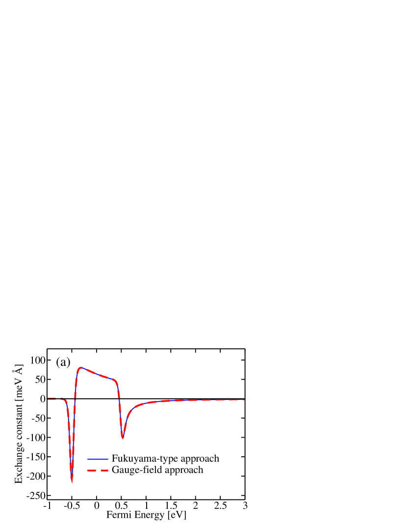
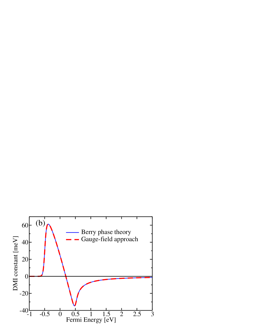
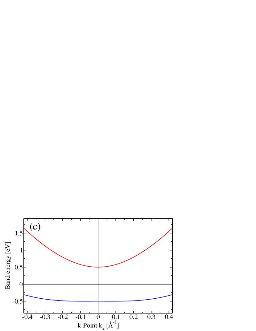
Figure 1: (a) Exchange constant $\mathscr{A}^{xx}$ and (b) DMI constant $D^{yx}$ in the one-dimensional Rashba model Eq. (69) as a function of Fermi energy for the model parameters $\Delta V=1$eV and $\alpha=2$eVÅ. Results obtained from the gauge-field approach (dashed lines) agree respectively to the exchange constant from the Fukuyama-type approach and to the DMI-constant from the Berry-phase approach (solid lines). (c) Band structure of the one-dimensional Rashba model.

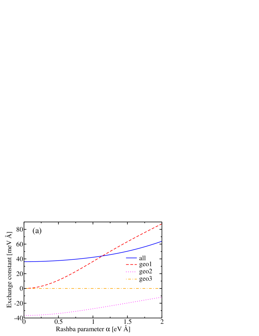
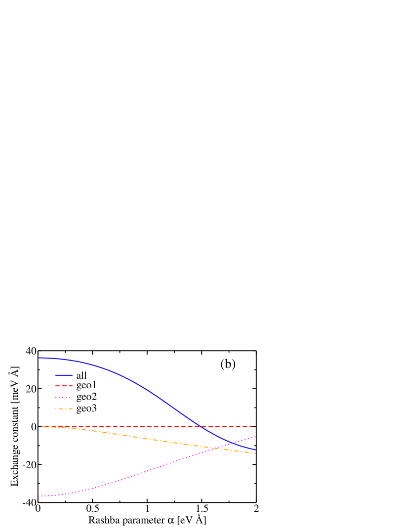
Figure 2: (a) Exchange constant $\mathscr{A}^{xx}$ and (b) $\mathscr{A}^{xy}$ in the one-dimensional Rashba model Eq. (69) as a function of the Rashba parameter $\alpha$. The Fermi energy is set to zero and $\Delta V=1$eV. Solid lines: Complete exchange constants. The geometrical contributions $\mathscr{A}_{\rm geo1}$ (dashed), $\mathscr{A}_{\rm geo2}$ (dotted), and $\mathscr{A}_{\rm geo3}$ (dashed-dotted) as defined in Eqs. (52) through (54) are shown as well.

In the presence of SOI both the exchange constant $\mathscr{A}^{ij}$ as obtained from Eq. (28) and the DMI constant $D^{ij}$ as obtained from Eq. (78) may depend on the magnetization direction $\hat{{\bm{n}}}$. However, as we explained in the discussion below Eq. (69), rotations in spin-space around the $y$ axis are a symmetry operation of the one-dimensional Rashba model. Since we consider the special case of a cycloidal spin-spiral, Eq. (56), which describes a magnetization that rotates around the $y$ axis as one moves along the spin-spiral, $\mathscr{A}^{ij}$ and $D^{ij}$ are constant along this spin-spiral. This allows us to compare the values of $\mathscr{A}^{ij}$ and $D^{ij}$ obtained for $\hat{{\bm{n}}}$ in $z$ direction to the values obtained from the gauge-field approach in this particular case, while in a general case a spin-spiral calculation will correspond to an $\hat{{\bm{n}}}$-integration of $\hat{{\bm{n}}}$-dependent $\mathscr{A}^{ij}$ and $D^{ij}$.

In Fig. 1 we show the exchange constant $\mathscr{A}^{xx}$ as well as the DMI coefficient for the one-dimensional Rashba model, Eq. (69), as a function of the Fermi energy. The parameters used in the model are $\Delta V=1$eV and $\alpha=2$eVÅ and we set the temperature in the Fermi functions to $k_{\rm B}T=25$ meV. Two approaches are compared: The dashed lines show the results obtained from Eq. (77) and Eq. (76) within the gauge-field approach, where we used a small spin-spiral vector of $q=0.006$ Å^-1 (we checked that making $q$ smaller does not affect the results). The solid line in Fig. 1(a) is obtained from the Fukuyama-type expression Eq. (28) for the exchange constant. The solid line in Fig. 1(b) is obtained from the Berry-phase theory of DMI, Eq. (78). The results from the different methods are in perfect agreement, which shows in particular that Eq. (28) can be used for calculating exchange constants even in the presence of SOI. The exchange constant becomes negative when the Fermi energy is close to $\pm 0.5$ eV, i.e., close to the band minima (see Fig. 1(c)). Negative exchange constants imply that the ferromagnetic state is unstable and that a spin-spiral state will form. With increasing Fermi energy, the effect of Rashba SOI on the Fermi surface becomes smaller and smaller. At very high Fermi energy the Fermi surfaces with an without SOI differ very little. As a consequence, the DMI is suppressed at high Fermi energy.

We have verified that the gauge-field approach, Eq. (76), and the Berry-phase theory, Eq. (78), agree at all orders in SOI. Previously, we have shown Freimuth et al. (2016) that the Berry-phase theory reduces to the ground-state spin current Kikuchi et al. (2016) at the first order in SOI.

In Fig. 2 we show the exchange constants $\mathscr{A}^{xx}$ and $\mathscr{A}^{xy}$ as a function of the Rashba parameter $\alpha$ when the Fermi energy is set to zero and $\Delta V=1$eV. $\mathscr{A}^{xx}$ is the exchange constant of a cycloidal spin-spiral and $\mathscr{A}^{xy}$ is the one of a helical spin-spiral. In the absence of SOI rotations in spin-space leave the spectrum of the Hamiltonian invariant and therefore $\mathscr{A}^{xx}=\mathscr{A}^{xy}$. For $\alpha\neq 0$ $\mathscr{A}^{xx}$ and $\mathscr{A}^{xy}$ differ from each other and the difference becomes large with increasing $\alpha$. The three geometrical contributions as defined in Eqs. (52) through (54) are shown in Fig. 2 as well. The mixed Berry curvature and the mixed quantum metric are zero without SOI and therefore we expect that $\mathscr{A}_{\rm geo1}$ and $\mathscr{A}_{\rm geo3}$, which depend on the mixed Berry curvature and the mixed quantum metric, differ between cycloidal and helical spin-spirals, which is indeed the case: While $\mathscr{A}^{xx}_{\rm geo1}$ increases strongly with $\alpha$, $\mathscr{A}^{xy}_{\rm geo1}$ is zero and while $\mathscr{A}^{xx}_{\rm geo3}$ is zero, $\mathscr{A}^{xy}_{\rm geo3}$ becomes negative with increasing $\alpha$. In contrast, $\mathscr{A}^{xx}_{\rm geo2}$ and $\mathscr{A}^{xy}_{\rm geo2}$ are very similar, because they only involve the quantum metric in real space as well as the inverse effective mass in $k$-space. Generally, the geometrical contribution cannot be neglected and is of the same order of magnitude as the total exchange constant.

The expressions Eq. (46), Eq. (47), and Eq. (48) contain both Fermi surface and Fermi sea terms. The exchange constant does not vanish in band insulators due to the Fermi sea terms and exhibits a plateau in the gap. To illustrate this we show in Fig. 3 the exchange constant of the one-dimensional Rashba model with model parameters $\alpha=20$eVÅ and $\Delta V=1$eV. In the $k_{x}$ integration we use a cutoff of 2.63Å^-1. This cutoff is necessary in order to obtain an insulating system because there is no global gap in the bandstructure of the one-dimensional Rashba model. However, when we restrict the range of $k$ points to the region -2.63Å${}^{-1}<k_{x}<$2.63Å^-1 the band structure appears gapped as shown in Fig. 3(a). As shown in Fig. 3(b) the corresponding exchange constant exhibits a plateau in the gap.

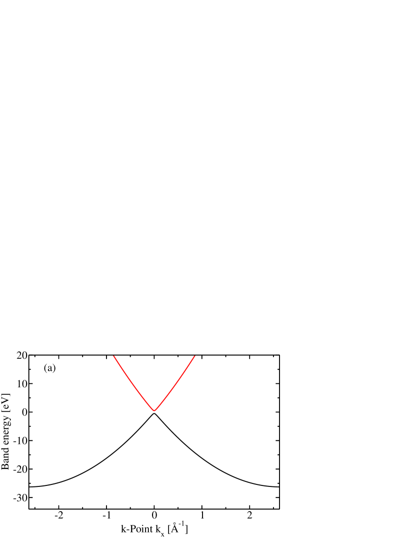
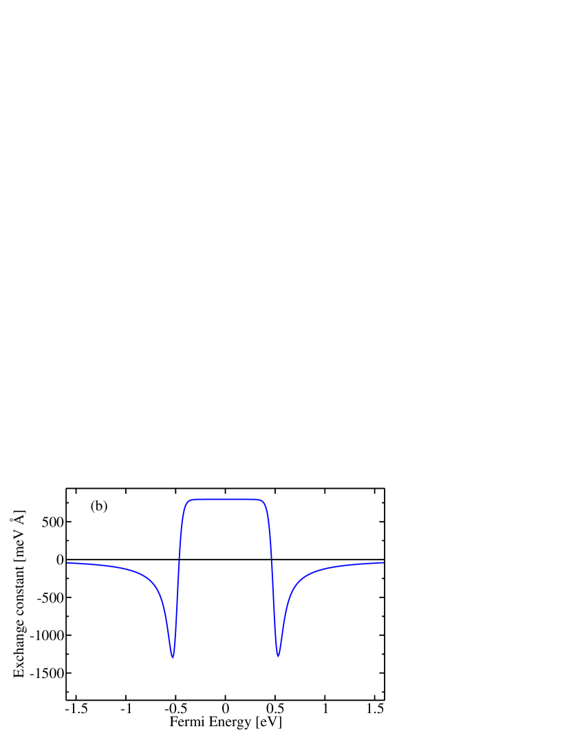
Figure 3: (a) Band energy of the one-dimensional Rashba model Eq. (69) with model parameters $\alpha=20$eVÅ and $\Delta V=1$eV. (b) The corresponding exchange constant exhibits a plateau between -0.3eV and 0.3eV due to the gap of the band structure in (a).

V.2 Rashba model in two dimensions

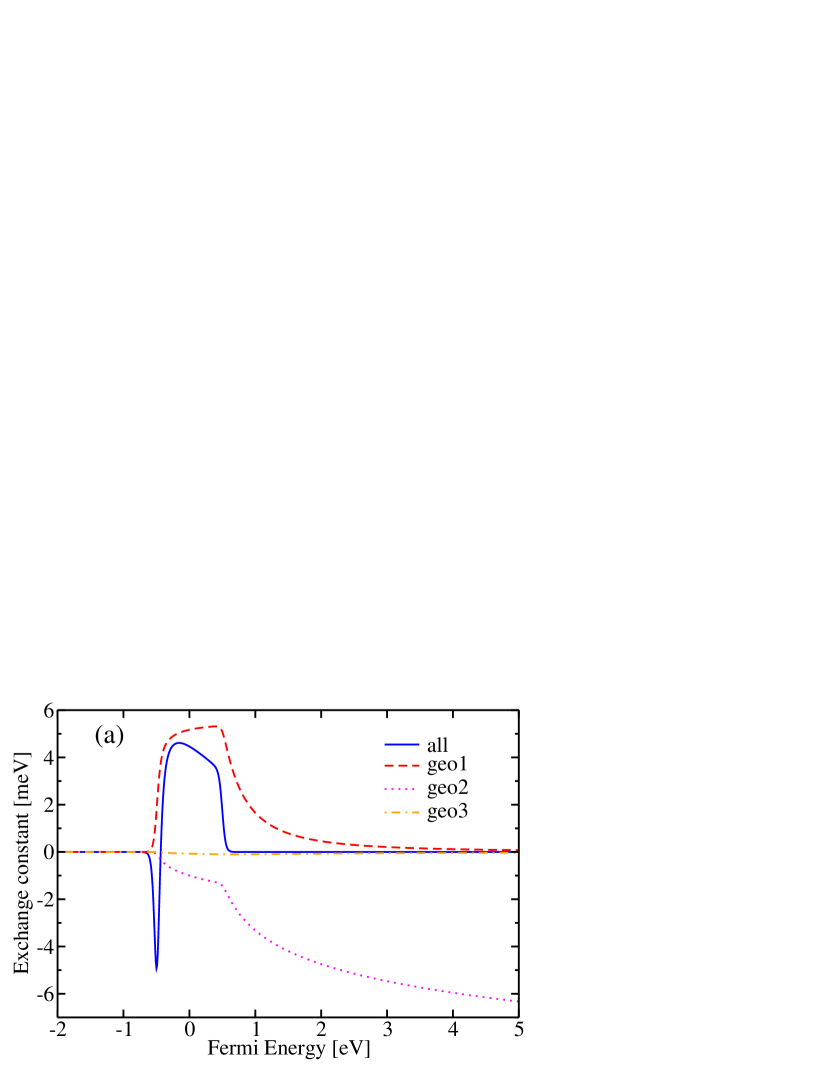
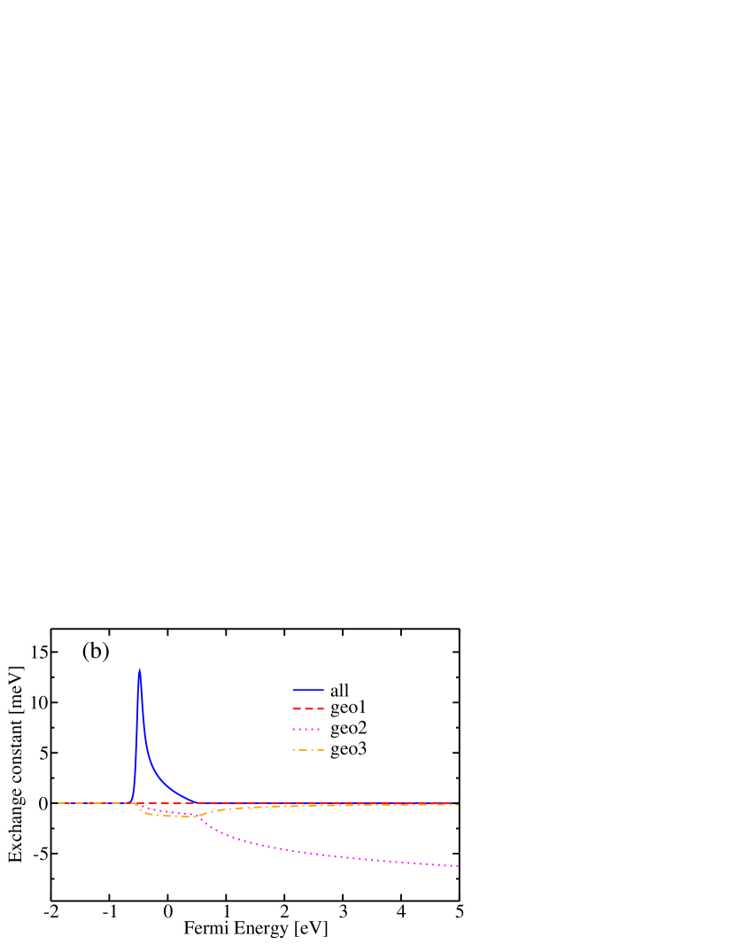
Figure 4: (a) Exchange constant $\mathscr{A}^{xx}$ and (b) $\mathscr{A}^{xy}$ in the two-dimensional Rashba model Eq. (55) as a function of the Fermi energy. The model parameters are $\alpha=2$eVÅ and $\Delta V=1$eV. Solid lines: Complete exchange constants. The geometrical contributions $\mathscr{A}_{\rm geo1}$ (dashed), $\mathscr{A}_{\rm geo2}$ (dotted), and $\mathscr{A}_{\rm geo3}$ (dashed-dotted) as defined in Eqs. (52) through (54) are shown as well.

When the Rashba parameter $\alpha$ is zero the exchange constant of the two-dimensional Rashba model can be obtained from the gauge-field approach as discussed in section IV.1. We checked that the gauge-field approach and Eq. (28) yield identical results in this case.

We now turn to the case with $\alpha>0$, where we use the model parameters $\alpha=2$eVÅ and $\Delta V=1$eV. In Fig. 4 we show the exchange constants $\mathscr{A}^{xx}$ and $\mathscr{A}^{xy}$ as obtained from Eq. (28) as a function of the Fermi energy, as well as the geometrical contributions $\mathscr{A}_{\rm geo1}$, $\mathscr{A}_{\rm geo2}$, and $\mathscr{A}_{\rm geo3}$ as defined in Eqs. (52) through (54). We rediscover several properties that we discussed already in the one-dimensional Rashba model: The exchange constant of the cycloidal spin-spiral ($\mathscr{A}^{xx}$) differs considerably from the exchange constant of the helical spin-spiral ($\mathscr{A}^{xy}$) when SOI is large. The contribution $\mathscr{A}_{\rm geo2}$ does not differ much between helical spin-spiral and cycloidal spin-spiral, while $\mathscr{A}_{\rm geo1}$ and $\mathscr{A}_{\rm geo3}$ are very different between these two cases.

VI Summary

We derive a formula that expresses the exchange constants in terms of Green’s functions, velocity operators, and torque operators of a collinear ferromagnet. Thus, it allows us to access the exchange constants directly from the electronic structure information without the need for spin-spiral calculations. We compare this formula to Fukuyama’s result for the orbital magnetic susceptibility and find strong formal similarities between these two theories. We rewrite the Green’s function expression for the exchange constant in terms of Berry curvatures and quantum metrices in mixed phase-space. Thereby we identify several geometrical contributions to the exchange constants that we find to be generally important in free electron model systems. Our formalism can be used even in the presence of spin-orbit interaction, where we find sizable differences between the exchange constants of helical and cycloidal spin spirals in the Rashba model.

Appendix A From torque-operator expressions to curvatures and geometrical quantities

In this appendix we discuss how to express matrix elements of the torque operator in terms of derivatives with respect to the magnetization direction. For this purpose we use that the Hamiltonian

$$H({\bm{r}})= -\frac{\hbar^{2}}{2m_{e}}\Delta+V({\bm{r}})+\mu_{\rm B}^{\phantom{B}}{\bm{\sigma}}\cdot\hat{{\bm{n}}}\Omega^{\rm xc}({\bm{r}})+$$ (82)

$$+\frac{1}{2ec^{2}}\mu_{\rm B}^{\phantom{B}}{\bm{\sigma}}\cdot\left[{\bm{\nabla}}V({\bm{r}})\times{\bm{v}}\right].$$

is dependent on the magnetization direction $\hat{{\bm{n}}}$ through the exchange interaction $\mu_{\rm B}{\bm{\sigma}}\cdot\hat{{\bm{n}}}\,\Omega^{\rm xc}({\bm{r}})$. The derivative of $H$ with respect to magnetization direction $\hat{{\bm{n}}}$ can be expressed in terms of the torque operator:

$$\hat{{\bm{n}}}\times\frac{\partial H}{\partial\hat{{\bm{n}}}}=\mu_{\rm B}\hat{{\bm{n}}}\times{\bm{\sigma}}\,\Omega^{\rm xc}({\bm{r}})=-\mu_{\rm B}{\bm{\sigma}}\times{\bm{\Omega}}^{\rm xc}({\bm{r}})={\bm{\mathcal{T}}}({\bm{r}}).$$ (83)

Thus, when the magnetization points in $z$ direction, i.e., when $\hat{{\bm{n}}}=\hat{{\bm{e}}}^{z}$, the cartesian components of ${\bm{\mathcal{T}}}$ are given by

$$\mathcal{T}^{x} =-\frac{\partial H}{\partial\hat{n}^{y}},$$ (84)

$$\mathcal{T}^{y} =\frac{\partial H}{\partial\hat{n}^{x}}.$$

Using

$$\frac{\partial|u_{{\bm{k}}n}\rangle}{\partial k^{x}} =\sum_{m\neq n}\frac{|u_{{\bm{k}}m}\rangle\langle u_{{\bm{k}}m}|\frac{\partial H({\bm{k}})}{\partial k^{x}}|u_{{\bm{k}}n}\rangle}{\mathcal{E}^{\phantom{R}}_{{\bm{k}}n}-\mathcal{E}^{\phantom{R}}_{{\bm{k}}m}}$$ (85)

$$+ia_{{\bm{k}}n}|u_{{\bm{k}}n}\rangle$$

$$=\hbar\sum_{m\neq n}\frac{|u_{{\bm{k}}m}\rangle\langle u_{{\bm{k}}m}|v^{x}({\bm{k}})|u_{{\bm{k}}n}\rangle}{\mathcal{E}^{\phantom{R}}_{{\bm{k}}n}-\mathcal{E}^{\phantom{R}}_{{\bm{k}}m}}$$

$$+ia_{{\bm{k}}n}|u_{{\bm{k}}n}\rangle$$

and

$$\frac{\partial|u_{{\bm{k}}n}\rangle}{\partial\hat{n}^{x}}= \sum_{m\neq n}\frac{|u_{{\bm{k}}m}\rangle\langle u_{{\bm{k}}m}|\frac{\partial H({\bm{k}})}{\partial\hat{n}^{x}}|u_{{\bm{k}}n}\rangle}{\mathcal{E}^{\phantom{R}}_{{\bm{k}}n}-\mathcal{E}^{\phantom{R}}_{{\bm{k}}m}}$$ (86)

$$+ib_{{\bm{k}}n}|u_{{\bm{k}}n}\rangle$$

$$=\sum_{m\neq n}\frac{|u_{{\bm{k}}m}\rangle\langle u_{{\bm{k}}m}|\mathcal{T}^{y}|u_{{\bm{k}}n}\rangle}{\mathcal{E}^{\phantom{R}}_{{\bm{k}}n}-\mathcal{E}^{\phantom{R}}_{{\bm{k}}m}}$$

$$+ib_{{\bm{k}}n}|u_{{\bm{k}}n}\rangle,$$

where the phases $a_{{\bm{k}}n}$ and $b_{{\bm{k}}n}$ determine the gauge, $H({\bm{k}})=e^{-i{\bm{k}}\cdot{\bm{r}}}He^{i{\bm{k}}\cdot{\bm{r}}}$ is the Hamiltonian in crystal momentum representation and $u_{{\bm{k}}n}({\bm{r}})=e^{-i{\bm{k}}\cdot{\bm{r}}}\psi_{{\bm{k}}n}({\bm{r}})$ is the lattice periodic part of the Bloch function $\psi_{{\bm{k}}n}({\bm{r}})$, we can express the mixed Berry curvature in terms of the torque operator and the velocity operator as follows:

$$\mathcal{B}^{xx}_{{\bm{k}}n}= -2\,{\rm Im}\left\langle\frac{\partial u_{{\bm{k}}n}}{\partial\hat{n}^{x}}\left|\frac{\partial u_{{\bm{k}}n}}{\partial k^{x}}\right.\right\rangle$$ (87)

$$= -2\hbar\,{\rm Im}\sum_{m\neq n}\frac{\langle\psi_{{\bm{k}}n}|\mathcal{T}^{y}|\psi_{{\bm{k}}m}\rangle\langle\psi_{{\bm{k}}m}|v^{x}|\psi_{{\bm{k}}n}\rangle}{(\mathcal{E}^{\phantom{R}}_{{\bm{k}}m}-\mathcal{E}^{\phantom{R}}_{{\bm{k}}n})^{2}}.$$

Similarly, we obtain an expression for the mixed quantum metric in terms of the torque operator and the velocity operator:

$$\mathcal{G}^{xx}_{{\bm{k}}n} ={\rm Re}\left[\frac{\partial\langle u_{{\bm{k}}n}|}{\partial\hat{n}^{x}}\Bigl{[}1-|u_{{\bm{k}}n}\rangle\langle u_{{\bm{k}}n}|\Bigr{]}\frac{\partial|u_{{\bm{k}}n}\rangle}{\partial k^{x}}\right]$$ (88)

$$=\hbar\,{\rm Re}\sum_{m\neq n}\frac{\langle\psi_{{\bm{k}}n}|\mathcal{T}^{y}|\psi_{{\bm{k}}m}\rangle\langle\psi_{{\bm{k}}m}|v^{x}|\psi_{{\bm{k}}n}\rangle}{(\mathcal{E}^{\phantom{R}}_{{\bm{k}}m}-\mathcal{E}^{\phantom{R}}_{{\bm{k}}n})^{2}}.$$

The quantum metric in magnetization space can be written as

$$\tilde{g}^{xx}_{{\bm{k}}n} ={\rm Re}\left[\frac{\partial\langle u_{{\bm{k}}n}|}{\partial\hat{n}^{x}}\Bigl{[}1-|u_{{\bm{k}}n}\rangle\langle u_{{\bm{k}}n}|\Bigr{]}\frac{\partial|u_{{\bm{k}}n}\rangle}{\partial\hat{n}^{x}}\right]$$ (89)

$$={\rm Re}\sum_{m\neq n}\frac{\langle\psi_{{\bm{k}}n}|\mathcal{T}^{y}|\psi_{{\bm{k}}m}\rangle\langle\psi_{{\bm{k}}m}|\mathcal{T}^{y}|\psi_{{\bm{k}}n}\rangle}{(\mathcal{E}^{\phantom{R}}_{{\bm{k}}m}-\mathcal{E}^{\phantom{R}}_{{\bm{k}}n})^{2}}.$$

The twist-torque moment of wavepackets is given by

$$\mathcal{A}^{xx}_{{\bm{k}}n} =-{\rm Im}\left\langle\frac{\partial u_{{\bm{k}}n}}{\partial\hat{n}^{x}}\right|\!\Bigl{[}\mathcal{E}_{{\bm{k}}n}-H_{{\bm{k}}}\Bigr{]}\!\left|\frac{\partial u_{{\bm{k}}n}}{\partial k^{x}}\right\rangle$$ (90)

$$=\hbar\,{\rm Im}\sum_{m\neq n}\frac{\langle\psi_{{\bm{k}}n}|\mathcal{T}^{y}|\psi_{{\bm{k}}m}\rangle\langle\psi_{{\bm{k}}m}|v^{x}|\psi_{{\bm{k}}n}\rangle}{(\mathcal{E}^{\phantom{R}}_{{\bm{k}}m}-\mathcal{E}^{\phantom{R}}_{{\bm{k}}n})}.$$

The interband Berry connection in magnetization space can be written as

$$\bar{A}^{x}_{{\bm{k}}mn} =i\langle u_{{\bm{k}}m}|\frac{\partial|u_{{\bm{k}}n}\rangle}{\partial\hat{n}^{x}}=$$ (91)

$$=i\frac{\langle u_{{\bm{k}}m}|\mathcal{T}^{y}|u_{{\bm{k}}n}\rangle}{\mathcal{E}^{\phantom{R}}_{{\bm{k}}n}-\mathcal{E}^{\phantom{R}}_{{\bm{k}}m}}.$$

The mixed phase-space analogue of the inverse effective mass tensor can be expressed in terms of the torque operator as

$$\bar{\alpha}^{xx}_{{\bm{k}}n} =\frac{\partial^{2}\mathcal{E}_{{\bm{k}}n}}{\partial k^{x}\partial\hat{n}^{x}}$$ (92)

$$=2\hbar\,{\rm Re}\sum_{m\neq n}\frac{\langle\psi_{{\bm{k}}n}|\mathcal{T}^{y}|\psi_{{\bm{k}}m}\rangle\langle\psi_{{\bm{k}}m}|v^{x}|\psi_{{\bm{k}}n}\rangle}{(\mathcal{E}^{\phantom{R}}_{{\bm{k}}n}-\mathcal{E}^{\phantom{R}}_{{\bm{k}}m})}.$$

Appendix B Analytical expressions when SOI is not included

In the following we derive analytical expressions for the case when SOI is not included in the Hamiltonian. When SOI is not included in the Hamiltonian, one can show that

$$\mathcal{T}^{y}=\frac{i}{2}[H,\sigma^{y}].$$ (93)

Inserting this identity into Eq. (89) one obtains the result

$$\tilde{g}^{xx}_{{\bm{k}}n}=\frac{1}{4}.$$ (94)

Inserting this result into Eq. (53) we get

$$\mathscr{A}_{\rm geo2}^{xx}=-\frac{1}{24}\frac{\hbar^{2}}{m_{e}}\mathcal{N},$$ (95)

where

$$\mathcal{N}=\int\!\!\frac{{\rm d}^{d}k}{(2\pi)^{d}}\sum_{n}f_{{\bm{k}}n}$$ (96)

is the electron density. In the case $d=2$ we have

$$\mathcal{N}=\frac{m\mathcal{E}_{\rm F}}{\pi\hbar^{2}},$$ (97)

if both majority and minority bands are occupied. If only the majority band is occupied we have instead

$$\mathcal{N}=\frac{m}{2\pi\hbar^{2}}\left[\mathcal{E}_{\rm F}+\frac{\Delta V}{2}\right].$$ (98)

$\mathscr{A}_{\rm geo2}^{xx}$ is the second term in Eq. (51). Similarly, the first term in Eq. (51) evaluates to

$$\int\!\!\frac{{\rm d}^{d}k}{(2\pi)^{d}}\sum_{n}\frac{1}{3}f_{{\bm{k}}n}\tilde{g}^{xx}_{{\bm{k}}n}\frac{\hbar^{2}}{m_{e}}=\frac{1}{12}\frac{\hbar^{2}}{m_{e}}\mathcal{N}.$$ (99)

The third term in Eq. (51) can be written as

$$-\frac{\hbar^{2}}{6}\int\!\!\frac{{\rm d}^{d}k}{(2\pi)^{d}}\sum_{n}f^{\prime}_{{\bm{k}}n}v_{{\bm{k}}n}^{x}\left\langle\frac{\partial u_{{\bm{k}}n}}{\partial\hat{n}^{x}}\right|[v^{x}_{{\bm{k}}}+v^{x}_{{\bm{k}}n}]\left|\frac{\partial u_{{\bm{k}}n}}{\partial\hat{n}^{x}}\right\rangle=$$ (100)

$$=-\frac{\hbar^{2}}{12}\int\!\!\frac{{\rm d}^{d}k}{(2\pi)^{d}}\sum_{n}f^{\prime}_{{\bm{k}}n}[v_{{\bm{k}}n}^{x}]^{2}.$$

When $d=2$ this becomes

$$\frac{\hbar^{4}}{48\pi m^{2}}\int k^{3}dk\sum_{n}\delta\left(\mathcal{E}_{\rm F}-\frac{\hbar^{2}k^{2}}{2m}-\frac{\Delta V}{2}s_{{\bm{k}}n}\right)$$ (101)

where $s_{{\bm{k}}n}=\pm 1$ denotes the spin (+1 for minority spin). When only the majority band is occupied this is equal to

$$\frac{1}{24\pi}\left[\mathcal{E}_{\rm F}+\frac{\Delta V}{2}\right]$$ (102)

and when both minority and majority bands are occupied it is equal to

$$\frac{1}{12\pi}\mathcal{E}_{\rm F}.$$ (103)

The interband Berry connection in magnetization space becomes:

$$\bar{A}^{x}_{{\bm{k}}mn}=\frac{1}{2}\langle u_{{\bm{k}}n}|\sigma^{y}|u_{{\bm{k}}n}\rangle.$$ (104)

Consequently, the fourth term in Eq. (51) can be written as

$$\frac{\hbar^{2}}{3}\int\!\!\frac{{\rm d}^{d}k}{(2\pi)^{d}}\sum_{n}f_{{\bm{k}}n}v^{x}_{{\bm{k}}n}v^{x}_{{\bm{k}}n}\sum_{m\neq n}\frac{\bar{A}^{x}_{{\bm{k}}mn}[\bar{A}^{x}_{{\bm{k}}mn}]^{*}}{\mathcal{E}_{{\bm{k}}n}-\mathcal{E}_{{\bm{k}}m}}=$$ (105)

$$=\frac{\hbar^{2}}{24\Delta V}\int\!\!\frac{{\rm d}^{d}k}{(2\pi)^{d}}\sum_{n}f_{{\bm{k}}n}s_{{\bm{k}}n}\frac{\hbar^{2}k^{2}}{m^{2}}=$$

$$=-\frac{1}{24\pi}\mathcal{E}_{\rm F},$$

where the last line holds only in the case $d=2$ when both majority and minority bands are occupied. When only the majority band is occupied we obtain in the case $d=2$ for the fourth term

$$-\frac{1}{96\pi}\left[\mathcal{E}_{\rm F}+\frac{\Delta V}{2}\right]-\frac{1}{48\pi}\frac{\mathcal{E}_{\rm F}}{\Delta V}\left[\mathcal{E}_{\rm F}+\frac{\Delta V}{2}\right].$$ (106)

The fifth term in Eq. (51) vanishes for the two-band model systems considered in this work.

For two-band models the sixth term in Eq. (51) is simply twice the fourth term.

The seventh term in Eq. (51) vanishes for the two-band model systems studied in this work.

Summing up all terms we obtain zero when both majority and minority bands are occupied. When only the majority band is occupied we obtain

$$\mathscr{A}^{xx}=\frac{1}{32\pi}\left[\mathcal{E}_{\rm F}+\frac{\Delta V}{2}\right]-\frac{3}{48\pi}\frac{\mathcal{E}_{\rm F}}{\Delta V}\left[\mathcal{E}_{\rm F}+\frac{\Delta V}{2}\right]$$ (107)

in the case $d=2$.

References

- Niu and Kleinman (1998) Q. Niu and L. Kleinman, Phys. Rev. Lett. 80, 2205 (1998).
- Niu et al. (1999) Q. Niu, X. Wang, L. Kleinman, W.-M. Liu, D. M. C. Nicholson, and G. M. Stocks, Phys. Rev. Lett. 83, 207 (1999).
- Qian and Vignale (2002) Z. Qian and G. Vignale, Phys. Rev. Lett. 88, 056404 (2002).
- Freimuth et al. (2014) F. Freimuth, S. Blügel, and Y. Mokrousov, Journal of physics: Condensed matter 26, 104202 (2014).
- Freimuth et al. (2013) F. Freimuth, R. Bamler, Y. Mokrousov, and A. Rosch, Phys. Rev. B 88, 214409 (2013).
- Freimuth et al. (2016) F. Freimuth, S. Blügel, and Y. Mokrousov, J. Phys.: Condens. matter 28, 316001 (2016).
- Freimuth et al. (2016) F. Freimuth, S. Blügel, and Y. Mokrousov, ArXiv e-prints (2016), eprint 1610.06541.
- Bruno et al. (2004) P. Bruno, V. K. Dugaev, and M. Taillefumier, Phys. Rev. Lett. 93, 096806 (2004).
- Fujita et al. (2011) T. Fujita, M. B. A. Jalil, S. G. Tan, and S. Murakami, Journal of applied physics 110, 121301 (2011).
- Resta (2010) R. Resta, J. Phys.: Condens. Matter 22, 123201 (2010).
- Fukuyama (1971) H. Fukuyama, Progress of Theoretical Physics 45, 704 (1971).
- Ogata and Fukuyama (2015) M. Ogata and H. Fukuyama, Journal of the Physical Society of Japan 84, 124708 (2015).
- Gao et al. (2015) Y. Gao, S. A. Yang, and Q. Niu, Phys. Rev. B 91, 214405 (2015).
- Piéchon et al. (2016) F. Piéchon, A. Raoux, J.-N. Fuchs, and G. Montambaux, Phys. Rev. B 94, 134423 (2016).
- Halilov et al. (1998) S. V. Halilov, H. Eschrig, A. Y. Perlov, and P. M. Oppeneer, Phys. Rev. B 58, 293 (1998).
- Kurz et al. (2004) P. Kurz, F. Förster, L. Nordström, G. Bihlmayer, and S. Blügel, Phys. Rev. B 69, 024415 (2004).
- Kohno et al. (2016) H. Kohno, Y. Hiraoka, M. Hatami, and G. E. W. Bauer, Phys. Rev. B 94, 104417 (2016).
- Şaşıoğlu et al. (2005) E. Şaşıoğlu, L. M. Sandratskii, P. Bruno, and I. Galanakis, Phys. Rev. B 72, 184415 (2005).
- Ležaić et al. (2013) M. Ležaić, P. Mavropoulos, G. Bihlmayer, and S. Blügel, Phys. Rev. B 88, 134403 (2013).
- Liechtenstein et al. (1987) A. Liechtenstein, M. Katsnelson, V. Antropov, and V. Gubanov, Journal of Magnetism and Magnetic Materials 67, 65 (1987).
- Bergqvist et al. (2004) L. Bergqvist, O. Eriksson, J. Kudrnovský, V. Drchal, P. Korzhavyi, and I. Turek, Phys. Rev. Lett. 93, 137202 (2004).
- Ebert and Mankovsky (2009) H. Ebert and S. Mankovsky, Phys. Rev. B 79, 045209 (2009).
- Jué et al. (2015) E. Jué, C. K. Safeer, M. Drouard, A. Lopez, P. Balint, L. Buda-Prejbeanu, O. Boulle, S. Auffret, A. Schuhl, A. Manchon, et al., Nature materials 15, 272 (2015).
- Akosa et al. (2016) C. A. Akosa, I. M. Miron, G. Gaudin, and A. Manchon, Phys. Rev. B 93, 214429 (2016).
- Gilmore et al. (2011) K. Gilmore, I. Garate, A. H. MacDonald, and M. D. Stiles, Phys. Rev. B 84, 224412 (2011).
- Franz et al. (2014) C. Franz, F. Freimuth, A. Bauer, R. Ritz, C. Schnarr, C. Duvinage, T. Adams, S. Blügel, A. Rosch, Y. Mokrousov, et al., Phys. Rev. Lett. 112, 186601 (2014).
- Raoux et al. (2015) A. Raoux, F. Piéchon, J.-N. Fuchs, and G. Montambaux, Phys. Rev. B 91, 085120 (2015).
- Gómez-Santos and Stauber (2011) G. Gómez-Santos and T. Stauber, Phys. Rev. Lett. 106, 045504 (2011).
- Sundaram and Niu (1999) G. Sundaram and Q. Niu, Phys. Rev. B 59, 14915 (1999).
- Xiao et al. (2005) D. Xiao, J. Shi, and Q. Niu, Phys. Rev. Lett. 95, 137204 (2005).
- Anandan and Aharonov (1990) J. Anandan and Y. Aharonov, Phys. Rev. Lett. 65, 1697 (1990).
- Neupert et al. (2013) T. Neupert, C. Chamon, and C. Mudry, Phys. Rev. B 87, 245103 (2013).
- Manchon et al. (2015) A. Manchon, H. C. Koo, J. Nitta, S. M. Frolov, and R. A. Duine, Nature materials 14, 871 (2015).
- Barke et al. (2006) I. Barke, F. Zheng, T. K. Rügheimer, and F. J. Himpsel, Phys. Rev. Lett. 97, 226405 (2006).
- Kikuchi et al. (2016) T. Kikuchi, T. Koretsune, R. Arita, and G. Tatara, Phys. Rev. Lett. 116, 247201 (2016).