On high-order conservative finite element methods

Abstract

We describe and analyze a volumetric and residual-based Lagrange multipliers saddle point reformulation of the standard high-order finite method, to impose conservation of mass constraints for simulating the pressure equation on two dimensional convex polygons, with sufficiently smooth solution and mobility phase. We establish high-order a priori error estimates with locally conservative fluxes and numerical results are presented that confirm the theoretical results.

1 Problem

Many porous media related practical problems lead to the numerical approximation of the pressure equation

$$-\mbox{div}(\Lambda(x)\nabla p)=q\quad\mbox{in}~{}~{}\Omega\subset\Re^{2},$$ (1)

$$p=0\quad\text{on}~{}~{}\partial\Omega_{D},$$ (2)

$$\nabla p\cdot\mathbf{n}=0\quad\text{on}~{}~{}\partial\Omega\backslash\partial\Omega_{D},$$ (3)

where $\partial\Omega_{D}$ is the part of the boundary of the domain $\Omega$ (denoted by $\partial\Omega$) where the Dirichlet boundary condition is imposed. In case the measure of $\partial\Omega_{D}$ (denoted by $|\partial\Omega_{D}|$) is zero, we assume the compatibility condition $\int_{\Omega}q\,dx=0$. On the above equation we have assumed without loss of generality homogeneous boundary conditions since we can always reduce the problem to that case. The domain $\Omega$ is assumed to be a convex polygonal region in order at least $H^{2}$ regularity, see [1], and for a rectangle domain the problem is $H^{p}$ regular for any integer $p$. We note however that this convexity or rectangularity are not required for the discretization, they are required only when regularity theory of partial differential equations (PDEs) is considered for establishing the a priori error estimates.

In multi-phase immiscible incompressible flow, $p$ and $\Lambda$ are the unknown pressure and the given phase mobitity of one of the phases in consideration (water, oil or gas); ( see e.g., [2, 3, 4, 5, 6, 7]). In general, the forcing term $q$ is due to gravity, phase transitions, sources and sinks, or when we transform a nonhomogeneous boundary condition problem to a homogeneous one. The mobility phase in consideration is defined by $\Lambda(x)=K(x)k_{r}(S(x))/\mu$, where $K(x)$ is the absolute (intrinsic) permeability of the porous media, $k_{r}$ is the relative phase permeability and $\mu$ the phase viscosity of the fluid. The assumptions required in this numerical analysis article may not in general hold for such large-scale flow models.

The main goal of our work is to obtain conservative solution of the equations above when they are discretized by high order continuous piecewise polynomial spaces. The obtained solution satisfies some given set of linear restrictions (may be related to subdomains of interest). Our motivations come from the fact that in some applications it is imperative to have some conservative properties represented as conservations of total flux in control volumes. For instance, if $\mathbf{q}^{h}$ represents the approximation to the flux (in our case $\mathbf{q}^{h}=-\Lambda\nabla p^{h}$ where $p^{h}$ is the approximation of the pressure), it is required that

$$\int_{\partial V}\mathbf{q}^{h}\cdot\mathbf{n}=\int_{V}q\quad\text{for each control volume}~{}~{}V.$$ (4)

Here $V$ is a control volume that does not cross $\partial\Omega_{D}$ from a set of controls volumes of interest, and here and after $\mathbf{n}$ is the normal vector pointing out the control volume in consideration. If some appropriate version of the total flux restriction written above holds, the method that produces such an approximation is said to be a conservative discretization.

Several schemes offer conservative discrete solutions. These schemes depend on the formulation to be approximated numerically. Among the conservative discretizations for the second the order formulation the elliptic problem we mention the finite volume (FV) method, some finite difference methods and some discontinuous Galerkin methods. On the other hand, for the first order formulation or the Darcy system we have the mixed finite element methods and some hybridizable discontinuous Galerkin (HDG) methods.

In this paper, we consider methods that discretize the second order formulation (1). Working with the second order formulation makes sense especially for cases where some form of high regularity holds. Usually in these cases the equality in the second order formulation is an equality in $L^{2}$ so that, in principle, there will be no need to weaken the equality by introducing less regular spaces for the pressure as it is done in mixed formulation with $L^{2}$ pressure.

For second order elliptic problems, a very popular conservative discretization is the finite volume (FV) method. The classical FV discretization provides and approximation of the solution in the space of piecewise linear functions with respect to a triangulation while satisfying conservation of mass on elements of a dual triangulation. When the approximation of the piecewise linear space is not enough for the problem at hand, advance approximation spaces need to be used (e.g., for problems with smooth solutions some high order approximation may be of interest). However, in some cases, this requires a sacrifice of the conservation properties of the FV method. Here in this paper, we design and analyze conservative solution in spaces of high order piecewise polynomials. We follow the methodology in [8], that imposes the total flux restrictions by employing Lagrange multiplier technique. This methodology was developed in order to apply the higher-order methods constructed in [9, 10, 11, 12] to two-phase flow problems.

We note that FV methods that use higher degree piecewise polynomials have been introduced in the literature. The fact that the dimension of the approximation spaces is larger than the number of restrictions led the researchers to design some method to select solutions: For instance, in [13, 14, 15] to introduce additional control volumes to match the number of restrictions to the number of unknowns. It is also possible to consider a Petrov-Galerkin formulation with additional test functions rather that only piecewise constant functions on the dual grid. Other approaches. have been also introduced, see for instance [16] and references therein.

In the construction of new methodologies into a reservoir simulation should have into account the following issues: 1) local mass conservation properties, 2) stable-fast solver and 3) the flexibility of re-use of the novel technique into more complex models (such as to nonlinear time-dependent transport equations equation for the convection dominated transport equation). For Darcy-like model problems with very high contrasts in heterogeneity, the discretization of Darcy-like models alone may be very hard to solve numerically due to a large condition number of the arising stiffness matrix. Moreover, the situation in even more intricate for modeling non trivial two- [17, 18] and three-phase [7, 6] transport convection dominated phenomena problems for flow through porous media (see also other relevant works [19, 2, 5, 20]). Thus, to achieve a sufficiently coupling between the volume fractions (or saturation) and the pressure-velocity, the full problem can be treated along with a fractional-step numerical procedure [7, 6]; we point out that we are aware about the very delicate issues linked to the discontinuous capillary-pressure (see [3] and the references therein). Indeed, the fluxes (Darcy velocities) are smooth at the vertices of the cell defining the integration volume in the dual triangularization, since these vertices are located at the centers of non-staggered cells, away from the jump discontinuities along the edges. This facilitates the construction of second-order and high-order approximations linked to the hyperbolic-parabolic model problem [7, 6]. This gives some of the benefits of staggering between primal and dual mesh triangulation by combining our novel high-order conservative finite element method with finite volume for hyperbolic-parabolic conservation laws modeling fluid flow in porous media applications.

Here in this paper, we consider a Ritz formulation and construct a solution procedure that combines a continuous Galerkin-type formulation that concurrently satisfies mass conservation restrictions. We impose finite volume restrictions by using a scalar Lagrange multiplier for each restriction. This is equivalently to a constraint minimization problem where we minimize the energy functional of the equation restricted to the subspace of functions that satisfy the conservation of mass restrictions. Then, in the Ritz sense, the obtained solution is the best among all functions that satisfy the mass conservation restriction.

Another advantage of our formulation is that the analysis can be carried out with classical tools for analyzing approximations to saddle point problems [21]. We analyze the method using an abstract framework and give an example for the case of second order piecewise polynomials. An important finding of these paper is that we were able to obtain optimal error estimates in the $H^{1}$ norm as well as the $L^{2}$ norm. Our $L^{2}$ error analysis requires additional assumptions, including specially collocated dual meshes and $\Lambda=I$, and is obtained by adding the Lagrange multipliers to the approximation $p_{h}$ by an Aubin-Nitsche trick [22, 23].

The rest of the paper is organized as follows. In Section 2 we present the Lagrange multipliers formulation of our problem. In Section 3 we introduce the saddle point approximation for which the analysis is presented in Section 4. In Section 5 we present the particular cases of high-order continuous finite element spaces. For this last case we present some numerical experiments in Section 6. To close the paper we present some conclusions in Section 7.

2 Lagrange multipliers and conservation of mass

Denote $H_{D}^{1}(\Omega)$ as the subspace of functions in $H^{1}(\Omega)$ which vanish on $\partial\Omega_{D}$. In case $|\partial\Omega_{D}|=0$, $H_{D}^{1}(\Omega)$ is the subspace of functions in $H^{1}(\Omega)$ with zero average on $\Omega$. The variational formulation of problem (1) is to find $p\in H^{1}_{D}(\Omega)$ such that

$$a(p,v)=F(v)\quad\mbox{ for all }v\in H_{D}^{1}(\Omega),$$ (5)

where the bilinear form $a$ is defined by

$$a(p,v)=\int_{\Omega}\Lambda(x)\nabla p(x)\cdot\nabla v(x)dx,$$ (6)

and the functional $F$ is defined by

$${F(v)=\int_{\Omega}q(x)v(x)dx.}$$ (7)

In order to consider a general formulation for porous media applications we let $\Lambda$ be a $2\times 2$ matrix with entries in $L^{\infty}(\Omega)$ in Problem (5) to be almost everywhere symmetric positive definite matrix with eigenvalues bounded uniformly from below by a positive constant, however, in certain parts of the paper when analysis and regularity theory are required, we assume $\Lambda(x)=I(identity)$. The Problem (5) is equivalent to the minimization problem: Find $p\in H_{D}^{1}$ and such that

$$p=\arg\min_{v\in H_{D}^{1}(\Omega)}\mathcal{J}(v),$$ (8)

where

$$\mathcal{J}(v)=\frac{1}{2}a(v,v)-F(v).$$ (9)

In order to deal with mass conservation properties we adopt the strategy introduced in [8]. Let us introduce the meshes we are going to use in our discrete problem. Let the primal triangulation ${\mathcal{T}}_{h}=\{R_{\ell}\}_{\ell=1}^{N_{h}}$ be made of elements that are triangles or squares and let $N_{h}$ be the number of elements of this triangulation. We also have a dual mesh ${\mathcal{T}}_{h}^{*}=\{V_{k}\}_{k=1}^{N^{*}_{h}}$ where the elements are called control volumes, and $N_{h}^{*}$ is the number of control volumes. Figure 1 illustrates a primal and dual mesh made of squares when $\partial\Omega_{D}=\partial\Omega$, and in this case $N^{*}_{h}$ is equal to the number of interior vertices of the primal triangulation. In general it is selected one control volume $V_{k}$ per vertex of the primal triangulation when the measure $|V_{k}\cap\partial\Omega_{D}|=0$. In case $|\partial\Omega_{D}|=0$, $N_{h}^{*}$ is the total number of vertices of the primal triangulation including the vertices on $\partial\Omega$.

In order to ensure the mass conservation, we impose it as a restriction (by using Lagrange multipliers) in each control volume $\{V_{k}\}_{k=1}^{N^{*}_{h}}$. We mention that our formulation allows for a more general case where only few control volumes, not necessarily related to the primal triangulation, are selected.

Let us define the linear functional $\tau_{k}(v)=\int_{\partial V_{k}}-\Lambda\nabla v\cdot\mathbf{n}\,ds$, $1\leq k\leq N^{*}_{h}$. We first note $\tau_{k}(v)$ is not well defined for $v\in H^{1}_{D}(\Omega)$. To fix that, recall that $q\in L^{2}(\Omega)$, therefore, let us define the Hilbert space

$${H^{1}_{div,\Lambda}(\Omega)}=\{v:v\in H_{D}^{1}(\Omega)\mbox{ and }\Lambda\nabla v\in\mbox{H}(\mbox{div},\Omega)\}$$

with norm $\|v\|_{H^{1}_{div,\Lambda}(\Omega)}^{2}=\|\Lambda\nabla v\cdot\nabla v\|_{L^{2}(\Omega)}^{2}+\|\mbox{div}(\Lambda\nabla v)\|^{2}_{L^{2}(\Omega)}$ where the divergence is taken in the weak sense. We note that this space and norm are well-defined with the properties of $\Lambda$ described above, that is, the smaller eigenvalue of $\Lambda(x)$ is uniformly bounded from below by a positive number, by using similar arguments given in  [24]*Theorem 1. It is easy to see by using integration by parts with the function $z=1$ that $\tau_{k}$ is a continuous linear functional on ${H^{1}_{div,\Lambda}(\Omega)}$. The integration by parts can be performed since $\|\Lambda\nabla v\cdot\nabla v\|_{L^{2}(V_{k})}^{2}+\|\mbox{div}(\Lambda\nabla v)\|^{2}_{L^{2}(V_{k})}$ is well-defined and bounded by $\|\Lambda\nabla v\cdot\nabla v\|_{L^{2}(\Omega)}^{2}+\|\mbox{div}(\Lambda\nabla v)\|^{2}_{L^{2}(\Omega)}$.

Let $p$ be the solution of (5) and define $m_{k}=\tau_{k}(p)=\int_{V_{k}}q\,ds$, $1\leq k\leq N_{h}^{*}$. The problem (8) is also equivalent to: Find $p\in{H^{1}_{div,\Lambda}(\Omega)}$ such that

$$p=\arg\min_{v\in\mathcal{W}}\mathcal{J}(v),$$ (10)

where

$$\mathcal{W}=\{v:v\in{H^{1}_{div,\Lambda}(\Omega)}\mbox{ such that }\tau_{k}(v)=m_{k},\quad 1\leq k\leq N^{*}_{h}\}.$$

Problem (10) above can be view as Lagrange multipliers min-max optimization problem. See [21] and references therein. Then, in case an approximation of $p$, say $p_{h}$ is required to satisfy the constraints $\tau_{k}(p^{h})=m_{k}$, $1\leq k\leq N^{*}_{h}$, we can do that by discretizing directly the formulation (10). In particular, we can apply this approach to a set of mass conservation restrictions used in finite volume discretizations.

In order to proceed with the associate Lagrange formulation, we define $M^{h}=\mathbb{Q}^{0}({\mathcal{T}}_{h}^{*})$ to be the space of piecewise constant functions on the dual mesh ${\mathcal{T}}_{h}^{*}$. For $\mu\in M^{h}$, depending on the context, we also interpret $\mu$ as the vector $[\mu_{k}]_{k=1}^{N_{h}^{*}}\in\mathbb{R}^{N_{h}^{*}}$ where $\mu_{k}=\mu|_{V_{k}}$. The Lagrange multiplier formulation of problem (10) can be written as: Find $p\in{H^{1}_{div,\Lambda}(\Omega)}$ and $\lambda\in M^{h}$ that solve:

$$\{p,\lambda\}=\arg\max_{\mu\in M^{h}}\min_{v\in{H^{1}_{div,\Lambda}(\Omega)},}\mathcal{J}(v)-(\overline{a}(p,\mu)-\overline{F}(\mu)).$$ (11)

Here, the total flux bilinear form $\overline{a}:{H^{1}_{div,\Lambda}(\Omega)}\times\,M^{h}\to\mathbb{R}$ is defined by

$$\overline{a}(v,\mu)=\sum_{k=1}^{N^{*}_{h}}\int_{\partial V_{k}}-\Lambda\nabla v\cdot\,\mathbf{n}\,\mu=\sum_{k=1}^{N^{*}_{h}}\mu_{k}\int_{\partial V_{k}}-\Lambda\nabla v\cdot\mathbf{n}\quad\mbox{ for all }v\in{H^{1}_{div,\Lambda}(\Omega)}\mbox{ and }\mu\in M^{h}.$$ (12)

The functional $\overline{F}:M^{h}\to\mathbb{R}$ is defined by

$$\overline{F}(\mu)=\sum_{i=k}^{N_{h}^{*}}\mu_{k}\int_{V_{k}}q\quad\mbox{ for all }\mu\in M^{h}.$$

Note that problem (11) depends on ${\mathcal{T}}_{h}^{*}$ and therefore depends on $h$. The first order conditions of the min-max problem above give the following saddle point problem: Find $p\in{H^{1}_{div,\Lambda}(\Omega)},$ and $\lambda\in M^{h}$ that solve:

$$\begin{array}[]{llr}a(p,v)+\overline{a}(v,\lambda)&=F(v)&\mbox{ for all }v\in{H^{1}_{div,\Lambda}(\Omega)},\\ \overline{a}(p,\mu)&=\overline{F}(\mu)&\mbox{ for all }\mu\in M^{h}.\\ \end{array}$$ (13)

See for instance [21]. Note that if the exact solution of problem (8) satisfies the restrictions in the saddle point formulation above we have $\lambda=0$ and we get the uncoupled system

$$\begin{array}[]{llr}a(p,v)&=F(v)&\mbox{ for all }v\in H^{1}_{div,\Lambda}(\Omega),\\ \overline{a}(p,\mu)&=\overline{F}(\mu)&\mbox{ for all }\mu\in M^{h}.\\ \end{array}$$ (14)

Also observe that the second equation above corresponds to a family of equations, one for each triangulation parametrized by $h$, all of them have the same solution.

3 Discretization

Recall that we have introduced a primal mesh ${\mathcal{T}}_{h}=\{R_{\ell}\}_{\ell=1}^{N_{h}}$ made of elements that are triangles or squares. We also have given a dual mesh ${\mathcal{T}}_{h}^{*}=\{V_{k}\}_{k=1}^{N^{*}_{h}}$ where the elements are called control volumes. In order to fix ideas we assume that the number of control volumes of ${\mathcal{T}}_{h}^{*}$ equals the number of free vertices of ${\mathcal{T}}_{h}^{*}$. Figure 1 illustrates a primal and dual mesh made of squares for the case $\partial\Omega_{D}=\partial\Omega$.

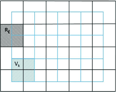
Figure 1: Example of regular mesh made of squares and its dual mesh for the case $\partial\Omega_{D}=\partial\Omega$.

Let us consider $P^{h}=\mathbb{Q}^{r}({\mathcal{T}}_{h})$ the space of continuous and piecewise polynomials of degree $r$ on each element of the primal mesh, and $P^{h}_{D}=P^{h}\cap H_{D}^{1}(\Omega)$ (which are the functions in $P^{h}$ that vanish in $\partial\Omega_{D}$). Let $M^{h}=\mathbb{Q}^{0}({\mathcal{T}}_{h}^{*})$ be the space of piecewise constant functions on the dual mesh ${\mathcal{T}}_{h}^{*}$. We mention here that our analysis may be extended to different spaces and differential equations. See for instance [8] where we consider GMsFEM spaces instead of piecewise polynomials.

The discrete version of (13) is to find $p^{h}\in P^{h}_{D}$ and $\lambda_{h}\in M^{h}$ such that

$$\begin{array}[]{llr}a(p^{h},v^{h})+\overline{a}(v^{h},\lambda^{h})&=F(v^{h})&\mbox{ for all }v^{h}\in P^{h}_{D},\\ \overline{a}(p^{h},\mu^{h})&=\overline{F}(\mu^{h})&\mbox{ for all }\mu^{h}\in M^{h}.\\ \end{array}$$ (15)

Let $\left\{\varphi_{i}\right\}$ be the standard basis of $P^{h}_{D}$. We define the matrix

$$A=\left[a_{i,j}\right]\quad\mbox{ where }a_{ij}=\int_{\Omega}\Lambda\nabla\varphi_{i}\cdot\nabla\varphi_{j}.$$ (16)

Note that $A$ is the finite element stiffness matrix corresponding to finite element space $P^{h}_{D}$. Introduce also the matrix

$$\overline{A}=\left[\overline{a}_{k,j}\right]\quad\mbox{ where }\overline{a}_{k,j}=\int_{\partial V_{k}}-\Lambda\nabla\varphi_{j}\cdot\textbf{n}.$$ (17)

With this notation, the matrix form of the discrete saddle point problem is given by,

$$\left[\begin{array}[]{cc}A&\overline{A}^{T}\\ \overline{A}&O\end{array}\right]\left[\begin{array}[]{c}p^{h}\\ \lambda^{h}\end{array}\right]=\left[\begin{array}[]{c}f\\ \overline{f}\end{array}\right]$$ (18)

where the vectors $f=[f_{i}]_{i=1}^{N_{h}}$ and $\overline{f}=[\overline{f}_{k}]_{k=1}^{N_{h}^{*}}$ are defined respectively by

$$f_{i}=\int_{\Omega}q\,\varphi_{i}\quad\mbox{ and }\quad\overline{f}_{k}=\int_{V_{k}}q.$$

For instance, in the case of the primal and dual triangulation of Figure 2 and polynomial degree $r=2$, the finite element matrix $A$ is a sparse matrix with 19 diagonals. Also, for a control volume $V_{k}$ there are at most $9$ supports of basis functions $\varphi_{j}$ with non-empty intersection with it, see Figure 2.

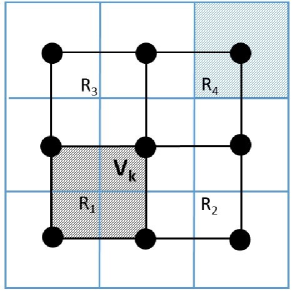
Figure 2: Control volumes that intersect the support of a $\mathbb{Q}^{2}({\mathcal{T}}_{h})$ basis function.

Remark 1.

Note that matrix $\overline{A}$ is related to classical (low order) finite volume matrix. Matrix $\overline{A}$ is a rectangular matrix with more columns than rows. Several previous works on conservative high-order approximation of second order elliptic problem have been designed by “adding” rows using several constructions. For instance, one can proceed as follows:

1. Construct additional control volumes and test the approximation spaces against piecewise constant functions over the total of control volumes (that include the dual grid element plus the additional control volumes). We mention that constructing additional control volumes is not an easy task and might be computationally expensive. We refer the interested reader to [13, 14, 15] for additional details.

2. Use additional basis functions that correspond to nodes other than vertices to obtain an FV/Galerkin formulation. This option has the advantage that no geometrical constructions have to be carried out. On the other hand, this formulation seems difficult to analyze. Also, some preliminary numerical tests suggest that the resulting linear system becomes unstable for higher order approximation spaces (especially for the case of high-contrast multiscale coefficients).

3. Use the Ritz formulation with restrictions (15).

Note that if piecewise polynomials of degree $r=1$ are used, in the linear system (18), the restriction matrix corresponds to the usual finite volume matrix. This matrix is known to be invertible. In this case, the affine space $\mathcal{W}$ is a singleton. Moreover, the only function $p_{h}$ satisfying the restriction is given by $p_{h}=(\overline{A})^{-1}\overline{f}$. The Ritz formulation (15) reduces to the classical finite volume method.

Then, in the Ritz sense, the solution of (15) is not worse than any of the solutions obtained by the method 1. or 2. mentioned above. Furthermore, the solution of the associated linear system (15), which is a saddle point linear system can be readily implemented using efficient solvers for the matrix $A$ (or efficient solvers for the classical finite volume matrix $\overline{A}$); See for instance [21]. Additionally, we mention that the analysis of the method can be carried out using usual tools for the analysis of restricted minimization of energy functionals and mixed finite element methods. The numerical analysis of our methodology is under current investigation and it will presented elsewhere.

4 Analysis

We show next that imposing the conservation in control volumes using Lagrange multipliers does not interfere with the optimality of the approximation in the $H^{1}$ norm. As we will see, imposing constraints will result in non optimal $L^{2}$ approximation but we were able to reformulate the $L^{2}$ approximation to get back to the optimal approximation by using the discrete Lagrange multiplier as a corrector.

Before proceeding we introduce notation to avoid proliferation of constants. We use the notation $A\preceq B$ to indicate that there is a constant $C_{1}$ such that $A\leq C_{1}B$. If additionally there exist $C_{2}$ such that $B\leq C_{2}A$ we write $A\asymp B$. These constants do not depend on $\Lambda$, $u$, $u_{h}$, $\lambda_{h}$, $q$, they might depend on the shape regularity of the elements and the shape of $\Omega$.

Denote $\|v\|^{2}_{a}=\int_{\Omega}\Lambda\nabla v\cdot\nabla v$ for all $v\in H^{1}_{D}(\Omega)$ and let us remind that $H^{1}_{div,\Lambda}:=\{v\in H^{1}_{D}(\Omega):\Lambda\nabla v\in\mbox{H}(\mbox{div},\Omega)\}$, and set $V^{h}=\mbox{Span}\{P_{D}^{h},H^{1}_{div,\Lambda}\}$. We present a concrete example of the norms of $V^{h}$ and $M^{h}$ in the next section, see (37) and (38), respectively.

Assumption A: There exist norms $\|\cdot\|_{V^{h}}$ and $\|\cdot\|_{M^{h}}$ for $V^{h}$ and $M^{h}$, respectively, such that

1. Augmented norm: $\|v\|_{a}\leq\|v\|_{V^{h}}$ forall $v\in V_{h}$.

2. Continuity: there exists $\|\bar{a}\|\in\mathbb{R}$ such that

   $$|\bar{a}(v,\mu^{h})|\leq\|\bar{a}\|\ \|v\|_{V^{h}}\|\mu^{h}\|_{M^{h}}~{}~{}\forall v\in V_{h}~{}~{}~{}\mbox{and}~{}~{}~{}\mu^{h}\in M^{h}.$$ (19)

3. Inf-Sup: there exists $\alpha>0$ such that

   $$\inf_{\mu^{h}\in M^{h}}\sup_{v^{h}\in P^{h}_{D}}\frac{\overline{a}(v^{h},\mu)}{\|v^{h}\|_{a}\,\|\mu^{h}\|_{M^{h}}}\geq\alpha>0.$$ (20)

Remark 2.

The Inf-Sup condition above can be replaced by: there exists $\alpha>0$ such that

$$\inf_{\mu^{h}\in M^{h}}\sup_{v^{h}\in P^{h}_{D}}\frac{\overline{a}(v^{h},\mu)}{\|v^{h}\|_{V^{h}}\,\|\mu^{h}\|_{M^{h}}}\geq\alpha>0.$$ (21)

We have the following result. Assume that $\{p,\lambda\}$ is the solution of (13) and $\{p_{h},\lambda_{h}\}$ the solution of (15). We have the following result. The proof uses classical approximation techniques for saddle point problems.

Theorem 3.

Assume that “Assumption A” holds. Then, there exists a constant $C$ such that

$$\|p-p^{h}\|_{a}\leqslant 2\left(1+\frac{\|\overline{a}\|}{\alpha}\right)\inf_{v^{h}\in P^{h}_{D}}\|p-v^{h}\|_{V^{h}}.$$

Proof.

Note that in both problems, (13) and (15), $\mu$ belongs to the finite dimensional subspace $M^{h}$. Also, the exact solution of the Lagrange multiplier component of (14) is $\lambda=0$. Now we derive error estimates following classical saddle point approximation analysis. Define

$$W^{h}(q):=\left\{v_{h}\in P^{h}_{D}:\overline{a}(v^{h},\mu)=\overline{F}(\mu)\,\,\mbox{ for all }\mu\in M^{h}\right\}$$

and

$$W^{h}:=\left\{v_{h}\in P^{h}_{D}:\overline{a}(v^{h},\mu)=0\,\,\mbox{ for all }\mu\in M^{h}\right\}.$$

First we prove

$$\|p-p^{h}\|_{a}\leq 2\inf_{w^{h}\in W^{h}(q)}\|p-w^{h}\|_{a}.$$ (22)

The inf-sup above in (20) implies that $W^{h}(q)$ (as well as $W^{h}$) is not empty. Take any $w^{h}\in W^{h}(q)$ and solve for $z^{h}$ the problem,

$$a(v^{h},z^{h})=F(z^{h})-a(w^{h},z^{h})\quad\mbox{ for all }z^{h}\in W_{h}.$$ (23)

Since $a$ is elliptic there exists a unique solution and therefore

$$p^{h}=v^{h}-w^{h},$$ (24)

where $p^{h}$ is the solution of (15). We have from (14) and (15) and using (23) that

$$a(v^{h},v^{h}) =a(p^{h}-w^{h},v^{h})$$

$$=a(p^{h},v^{h})-a(w^{h},v^{h})$$

$$={F(v^{h})}-a(w^{h},v^{h})$$

$$=a(p,v^{h})-a(w^{h},v^{h})$$

$$=a(p-w^{h},v^{h}).$$

Then, by using the ellipticity of $a$, we have

$$\|v^{h}\|^{2}_{a}=a(v^{h},v^{h})=a(p-w^{h},v^{h})\leqslant\|p-w^{h}\|_{a}\|v^{h}\|_{a}.$$ (25)

Then

$$\|p-p^{h}\|_{a} \leqslant\|p-w^{h}\|_{a}+\|w^{h}-p^{h}\|_{a}$$

$$\leqslant\|p-w^{h}\|_{a}+\|p-w^{h}\|_{a}=2\|p-w^{h}\|_{a}$$

so that (22) holds true.

We now show that

$$\inf_{w^{h}\in W^{h}(q)}\|p-w^{h}\|_{a}\leqslant\left(1+\frac{\|\overline{a}\|}{\alpha}\right)\inf_{v^{h}\in P^{h}_{D}}\|p-v^{h}\|_{V^{h}}$$ (26)

Take any $v^{h}\in W^{h}$. The inf-sup condition (20) implies that there exists a unique $z^{h}\in P^{h}_{D}$ such that

$$\overline{a}(z^{h},\mu)=\overline{a}(p-v^{h},\mu) \mbox{for all }\mu\in M^{h}.$$

Then we have that $z^{h}\neq 0$,

$$\frac{\overline{a}(z^{h},\mu)}{\|z^{h}\|_{a}\|\mu\|_{M^{h}}}\geq\alpha$$

and therefore

$$\|z^{h}\|_{a} \leqslant\frac{1}{\alpha}\cdot\frac{\overline{a}(z^{h},\mu)}{\|\mu^{h}\|}=\frac{1}{\alpha}\cdot\frac{\overline{a}(p-v^{h},\mu)}{\|\mu\|_{M^{h}}}$$

$$\leqslant\frac{1}{\alpha}\|\overline{a}\|\|p-v^{h}\|_{V^{h}}.$$

Note that we have used the continuity of $\bar{a}$ in the extended norm $\|\cdot\|_{V^{h}}$. Put $w^{h}=z^{h}+v^{h}$ then

$$\overline{a}(w^{h},\mu) =\overline{a}(z^{h},\mu)+\overline{a}(v^{h},\mu)$$

$$=\overline{a}(p-v^{h},\mu)+\overline{a}(v^{h},\mu)$$

$$=\overline{a}(p,\mu)$$

$$=\overline{F}(\mu).$$

Therefore we have that $w^{h}\in W_{h}(q)$. Moreover,

$$\|p-w^{h}\|_{a} \leqslant\|p-v^{h}\|_{a}+\|v^{h}-w^{h}\|_{a}$$

$$\leqslant\|p-v^{h}\|_{a}+\|z_{h}\|_{a}$$

$$\leqslant\|p-v^{h}\|_{a}+\frac{\|\overline{a}\|}{\alpha}\,\|p-v^{h}\|_{V^{h}}$$

$$\leqslant\left(1+\frac{\|\overline{a}\|}{\alpha}\right)\|p-v^{h}\|_{V^{h}}.$$

Combining (22) and (26) we get the result. ∎

From now on we assume from that $\Lambda=I$ (identity). In this case, $\|\cdot\|_{a}=|\cdot|_{H^{1}(\Omega)}$, and as we will see in Section 5 for regular meshes and $\mathbb{Q}^{r}({\mathcal{T}}_{h})$ elements that the “Assumption A” holds with $1/\alpha=O(1)$, $|\bar{a}|=O(1)$ with the norms $V^{h}$ and $M^{h}$ defined in (37) and (38), respectively. The next two Assumptions are discussed at the end of Section 5.

Assumption B: Assume that solution $p$ of the problem (1) is in $H^{r+1}(\Omega)$ and the following approximation holds for some integer $r\leq 1$

$$\inf_{v_{h}\in P^{h}_{D}}\|p-v_{h}\|_{V^{h}}\preceq h^{r}|p|_{H^{r+1}(\Omega)}.$$

As a corollary of “Assumptions A and B” and Lemma 3, we obtain

$$\|p-p^{h}\|_{V^{h}}\preceq h^{r}|p|_{H^{r+1}(\Omega)}.$$

As we will show in the numerical experiments, the error $\|p-p^{h}\|_{L^{2}(D)}$ is not optimal but according to the next result if we correct $p^{h}$ to $p^{h}+\lambda^{h}$ we recover the optimal approximation. The proof of the following results follows from a duality argument similar to that of the Aubin-Nitsche method; see [22, 23]. Let us introduce the following regularity assumption:

Assumption C: The problem is $H^{2}(\Omega)$ regular (see [22]) if for any $\tilde{q}\in L^{2}(\Omega)$ as a right-hand side for the problem (1), its solution $\tilde{p}$ satisfies

$$\|\tilde{p}\|_{H^{2}(\Omega)}\preceq\|\tilde{q}\|_{L^{2}(\Omega)}.$$

Theorem 4.

Assume that $\Lambda=I$. Assume also that “Assumptions A, B and C” hold. Then,

$$\|p-(p^{h}+\lambda^{h})\|_{L^{2}(\Omega)}\preceq h^{r+1}|p|_{H^{r+1}(\Omega)}.$$

Proof.

For $g\in L^{2}$ define $\mathcal{S}^{h}_{1}g$ and $\mathcal{S}^{h}_{0}g$ as the solution of

$$a(\mathcal{S}^{h}_{1}g,v^{h})+\overline{a}(v^{h},\mathcal{S}^{h}_{0}g)=\int_{D}gv^{h} \mbox{ for all }v^{h}\in H^{1}_{div,I}$$ (27)

$$\overline{a}(\mathcal{S}^{h}_{1}g,\mu)=\int_{D}gv^{h}\mu \mbox{ for all }\mu\in M^{h}.$$ (28)

Analogously, define $Sg$ as the solution of

$$\begin{array}[]{llr}a(Sg,v)&=\int_{D}gv&\mbox{ for all }v\in H^{1}_{div,I},\\ \overline{a}(Sg,\mu^{h})&=\int_{D}g\mu^{h}&\mbox{ for all }\mu^{h}\in M^{h}.\\ \end{array}$$ (29)

Observe that $p^{h}=S^{h}_{1}q$, $\lambda^{h}=S^{h}_{0}q$ and $p=Sq$. According to our previous result in Theorem 3 combined with standard regularity and approximation results ([22]) we have

$$||Sg-S^{h}_{1}g||_{a}\preceq\inf_{v^{h}\in P^{h}_{D}}||Sg-v^{h}||_{V^{h}}\preceq h||Sg||_{H^{2}(\Omega)}\preceq h||g||_{L^{2}(\Omega)}.$$ (30)

Recall that,

$$\|p-(p^{h}+\lambda^{h})\|_{L^{2}(\Omega)}=\sup_{g\in L^{2}}\frac{(p-(p^{h}+\lambda^{h}),g)}{\|g\|_{L^{2}(\Omega)}}.$$ (31)

By using the definition of $S$, $S^{h}_{0}$ and $S^{h}_{1}$ in (27) and (29) we get

$$(p-(p^{h}+\lambda^{h}),g)=(p,g)_{0}-(p^{h},g)_{0}-(\lambda^{h},g)_{0}$$

$$=a(Sg,p)-\Big{(}a(S^{h}_{1}g,p^{h})_{0}+\overline{a}(p^{h},S_{0}^{h}g)\Big{)}-\overline{a}(S_{1}^{h}g,\lambda^{h})$$

$$=a(Sg,p)-\Big{(}a(S^{h}_{1}g,p^{h})_{0}+\overline{a}(S_{1}^{h}g,\lambda^{h})\Big{)}-\overline{a}(p^{h},S_{0}^{h}g)$$

$$=a(Sg,p)-\left(\int_{D}fS^{h}_{1}g\right)-\overline{a}(p^{h},S_{0}^{h}g)$$

$$=a(Sg,p)-a(p,S^{h}_{1}g)-\overline{a}(p^{h},S_{0}^{h}g)$$

$$=a(p,Sg-S^{h}_{1}g)-\overline{a}(p^{h},S_{0}^{h}g)$$

$$=a(p-p^{h},Sg-S^{h}_{1}g)+a(p^{h},Sg-S^{h}_{1}g)-\overline{a}(p^{h},S_{0}^{h}g)$$

$$=a(p-p^{h},Sg-S^{h}_{1}g)+a(p^{h},Sg)-\Big{(}a(S^{h}_{1}g,p^{h})-\overline{a}(p^{h},S_{0}^{h}g)\Big{)}$$

$$=a(p-p^{h},Sg-S^{h}_{1}g)+\int_{D}gp^{h}-\left(\int_{D}gp^{h}\right)$$

$$=a(p-p^{h},Sg-S^{h}_{1}g)$$

$$\leq||p-p^{h}||_{a}||Sg-S^{h}_{1}g||_{a}$$

$$\preceq h|p-p^{h}|_{a}||g||_{L^{2}(\Omega)}$$

In the last step we have used (30). Replacing the last inequality in (31) and with “Assumption B”, we get the result. ∎

5 The case of piecewise polynomials of degree two in regular meshes

In this section we consider a regular mesh made of squares. See Figure 1. Define

$$\Gamma^{*}_{h}=\bigcup_{k=1}^{N^{*}_{h}}\partial V_{k}=\bigcup_{k,k^{\prime}=1}^{N^{*}_{h}}(\partial V_{k}\cap\partial V_{k^{\prime}})$$

that is, $\Gamma^{*}_{h}$ is the interior interface generated by the dual mesh. For $\mu\in M^{h}$ define $[\mu]$ on $\Gamma^{*}_{h}$ as the jump across element interfaces, that is, $[\mu]|_{\partial V_{k}\cap\partial V_{k^{\prime}}}=\mu_{k}-\mu_{k^{\prime}}$. Note that for $p\in V^{h}$

$$\overline{a}(p,{\mu}) =\sum_{k=1}^{N^{*}_{h}}\mu_{k}\int_{\partial V_{k}}-\nabla p\cdot\mathbf{n}=\int_{\Gamma^{*}_{h}}-\nabla p\cdot\mathbf{n}\,\left[\mu\right].$$

For each control volume $V_{k}$, denote by $E(k)$ the set of element of the primal mesh that intersect $V_{k}$. Note that in each control volume we have

$$\int_{\partial V_{k}}-\nabla p\cdot\mathbf{n}=\sum_{\ell\in E(k)}\int_{\partial V_{k}\cap R_{\ell}}-\nabla p\cdot\mathbf{n}.$$

To motivate the definition of the norms we study the continuity of the bilinear form $\overline{a}$. Observe that,

$$\left(\int_{\partial V_{k}\cap\partial V_{k^{\prime}}}-\nabla p\cdot\mathbf{n}\,\left[{\mu}\right]\right)^{2} \leq\left(h\int_{\partial V_{k}\cap\partial V_{k^{\prime}}}(\nabla p\cdot\mathbf{n})^{2}\right)\,\left(\frac{1}{h}\int_{\partial V_{k}\cap\partial V_{k^{\prime}}}[\mu]^{2}\right).$$

And therefore by applying Cauchy inequality and adding up we get,

$$|\overline{a}(p,{\mu})|\leq\left(h\int_{\Gamma^{*}_{h}}(\nabla p\cdot\mathbf{n})^{2}\right)^{1/2}\left(\frac{1}{h}\int_{\Gamma^{*}_{h}}[\mu]^{2}\right)^{1/2}.$$

Using a trace inequality we get that

$$h\int_{\Gamma^{*}_{h}}(\nabla p\cdot\mathbf{n})^{2} =h\sum_{k=1}^{N^{*}_{h}}\int_{\partial V_{k}}(\nabla p\cdot\mathbf{n})^{2}$$ (32)

$$=\sum_{k=1}^{N^{*}_{h}}\sum_{\ell\in E(k)}h\int_{\partial V_{k}\cap R_{\ell}}(\nabla p\cdot\mathbf{n})^{2}$$ (33)

$$\preceq\sum_{k=1}^{N^{*}_{h}}\sum_{\ell\in E(k)}\left(|p|^{2}_{H^{1}(V_{k}\cap R_{\ell})}+h^{2}(\|p_{xx}\|^{2}_{L^{2}(V_{k}\cap R_{\ell})}+\|p_{yy}\|^{2}_{L^{2}(V_{k}\cap R_{\ell})})\right)$$ (34)

$$=\sum_{\ell=1}^{N_{h}}\left(|p|_{H^{1}(R_{\ell})}^{2}+h^{2}(\|p_{xx}\|^{2}_{L^{2}(R_{\ell})}+\|p_{yy}\|^{2}_{L^{2}(R_{\ell})})\right)$$ (35)

$$=|p|_{H^{1}(\Omega)}^{2}+h^{2}\sum_{\ell=1}^{N_{h}}(\|p_{xx}\|^{2}_{L^{2}(R_{\ell})}+\|p_{yy}\|^{2}_{L^{2}(R_{\ell})}).$$ (36)

Now we are ready to define the norm

$$\|p\|^{2}_{V^{h}}=|p|^{2}_{H^{1}(\Omega)}+h^{2}\sum_{\ell=1}^{N_{h}}(\|p_{xx}\|^{2}_{L^{2}(R_{\ell})}+\|p_{yy}\|^{2}_{L^{2}(R_{\ell})})$$ (37)

Note that if $p\in\mathbb{Q}^{1}({\mathcal{T}}_{h})$ then $\|p\|_{V^{h}}^{2}=|p|^{2}_{H^{1}(\Omega)}$. Also, if $p\in\mathbb{Q}^{2}({\mathcal{T}}_{h})$ we have $\|p\|_{V^{h}}^{2}\leq c|p|^{2}_{H^{1}(\Omega)}$ by using inverse inequality.

Also define the discrete norm for the spaces of Lagrange multipliers as

$$\|{\mu}\|_{M^{h}}^{2}=\frac{1}{h}\int_{\Gamma^{*}_{h}}[\mu]^{2}.$$ (38)

We have shown above that the form $\overline{a}$ is continuous, that is, there is a constant $|\bar{a}|$ such that,

$$|\overline{a}(p,{\mu})|\leq|\bar{a}\|p\|_{V^{h}}\|{\mu}\|_{M^{h}}.$$

This also implies continuity in the $H^{1}$ norm. Now let us show the inf-sup condition.

Theorem 5.

Consider the norms for $\|\cdot\|_{a}=|\cdot|_{H^{1}(\Omega)}$ and $M^{h}$ defined in (38), respectively. There is a constant $\alpha$ such that,

$$\inf_{\mu\in M^{h}}\sup_{v^{h}\in\mathbb{Q}^{1}({\mathcal{T}}_{h})}\frac{\overline{a}(v^{h},\mu)}{\|v^{h}\|_{a}\,\|\mu\|_{M^{h}}}\geq\alpha>0.$$ (39)

Proof.

Given ${\mu}\in M^{h}$ define $v\in\mathbb{Q}^{1}({\mathcal{T}}_{h})$ as $v(x_{i})=\overline{\mu}(x_{i})$ if $x_{i}$ is a vertex of the primal mesh in $V_{i}$ and $v(x_{i})=0$ if $x_{i}$ is a vertex of the primal mesh on $\partial\Omega_{D}$. We first verify that,

$$|v|_{H^{1}}^{2}=\|v\|_{V^{h}}^{2}\asymp\|{\mu}\|_{M^{h}}^{2}.$$ (40)

It is enough to verify this equivalence of norms in the reference square $\hat{R}=[0,1]\times[0,1]$. Denote by $P_{i}$, $i=1,2,3,4$ the values of the reference function $\hat{v}$ at the nodes of the reference element. We have,

$$\hat{v}=P_{1}(1-x)(1-y)+P_{2}(x)(1-y)+P_{3}(1-x)y+P_{4}xy,\\$$

and we can directly compute $\partial_{x}\hat{v}=(P_{2}-P_{1})(1-y)+(P_{4}-P_{3})y$ and $\partial_{y}\hat{v}=(P_{3}-P_{1})(1-x)+(P_{4}-P_{2})x$. Therefore, after some calculations we obtain

$$(P_{2}-P_{1})^{2}\frac{1}{6}+(P_{4}-P_{3})^{2}\frac{1}{6} \leq(P_{2}-P_{1})^{2}\frac{1}{3}+(P_{4}-P_{3})^{2}\frac{1}{3}-|(P_{2}-P_{1})(P_{4}-P_{3})|\frac{1}{3}$$

$$\leq\int_{\hat{R}}(\partial_{x}\hat{v})^{2}$$

$$\leq(P_{2}-P_{1})^{2}\frac{1}{3}+(P_{4}-P_{3})^{2}\frac{1}{3}+|(P_{2}-P_{1})(P_{4}-P_{3})|\frac{1}{3}$$

$$\leq(P_{2}-P_{1})^{2}\frac{1}{2}+(P_{4}-P_{3})^{2}\frac{1}{2}.$$

Analogously,

$$(P_{3}-P_{1})^{2}\frac{1}{6}+(P_{4}-P_{2})^{2}\frac{1}{6}\leq\int_{R}(\partial_{y}\hat{v})^{2}\leq(P_{3}-P_{1})^{2}\frac{1}{2}+(P_{4}-P_{2})^{2}\frac{1}{2}.$$

This prove (40). Now we verify that

$$\int_{\Gamma^{*}_{h}}\nabla v\cdot\mathbf{n}[{\mu}]\succeq\|\mu\|_{M^{h}}^{2}.$$

Observe that if $R$ is an element of the primal triangulation, $\Gamma^{*}_{h}\cap R$ can be written as the union of four segments denoted by $\Gamma^{*}_{i,R}$ where $i=4(up),2(left),3(right),1(down)$. Working again on the reference square, we have

$$\int_{\hat{\Gamma}^{*}_{1,\hat{R}}}\nabla\hat{v}\cdot\mathbf{n}[P_{2}-P_{1}] =(P_{2}-P_{1})\int_{0}^{1/2}(P_{2}-P_{1})(1-y)+(P_{4}-P_{3})y$$

$$=(P_{2}-P_{1})^{2}\frac{3}{8}+(P_{2}-P_{1})(P_{4}-P_{3})\frac{1}{8}.$$

Analogously,

$$\int_{\hat{\Gamma}^{*}_{2,\hat{R}}}\nabla\hat{v}\cdot\mathbf{n}[P_{4}-P_{3}] =(P_{4}-P_{3})^{2}\frac{3}{8}+(P_{2}-P_{1})(P_{4}-P_{3})\frac{1}{8}$$

$$\int_{\hat{\Gamma}^{*}_{3,\hat{R}}}\nabla\hat{v}\cdot\mathbf{n}[P_{3}-P_{1}] =(P_{3}-P_{1})^{2}\frac{3}{8}+(P_{3}-P_{1})(P_{4}-P_{2})\frac{1}{8}$$

$$\int_{\hat{\Gamma}^{*}_{4,\hat{R}}}\nabla\hat{v}\cdot\mathbf{n}[P_{4}-P_{2}] =(P_{4}-P_{2})^{2}\frac{3}{8}+(P_{3}-P_{1})(P_{4}-P_{2})\frac{1}{8}$$

If we add these last form equations we get

$$\int_{\Gamma^{*}_{h}\cap R}\nabla v\cdot\mathbf{n}[{\mu}]\succeq(P_{2}-P_{1})^{2}+(P_{3}-P_{1})^{2}+(P_{4}-P_{2})^{2}+(P_{4}-P_{3})^{2}.$$

This finish our proof. ∎

We mention that for quasi-uniform and shape regular meshes, for quadrilateral $\mathbb{Q}^{r}({\mathcal{T}}_{h})$ or triangular $\mathbb{P}^{r}({\mathcal{T}}_{h})$ finite element spaces, the “Assumption B” holds for $p\in H^{r+1}(\Omega)$. For the solution $p$ of problem (1) to be in $H^{r+1}(\Omega)$, it is necessary to impose conditions on the shape and smoothness of domain as well as on the type of boundary conditions (Dirichlet, Neumann or mixed); see [1]. For instance, for the pure homogeneous Dirichlet boundary condition case, it is sufficient that $\Omega$ be convex and $q\in L^{2}(\Omega)$ in order that $p\in H^{2}(\Omega)$, and also “Assumption C” follows. For $p$ to be in $H^{r+1}(\Omega)$ for integer $r\leq 2$, it is sufficient that $\Omega$ be a rectangular domain and $q\in H^{r-1}(\Omega)$. Higher-order approximation and regularity can also be obtained for curved isoparametric finite elements on domains with smooth boundaries.

6 Numerical Experiments

We consider the Dirichlet problem (1) and employ the meshes depicted in Figure 1 with a variety of mesh sizes and $\Lambda=I$. We impose conservation of mass as described in the paper by using Lagrange multipliers. For this paper, we solved the saddle point linear system by LU decomposition. Several iterative solvers can be proposed for this saddle point problem but this will be considered in future studies, not here.

Consider $\Omega=[0,1]\times[0,1]$ and $\Lambda=I$. We consider a regular mesh made of $2^{M}\times 2^{M}$ squares. The dual mesh is constructed by joining the centers of the elements of the primal mesh. We performed a series of numerical experiments to compare properties of FEM solutions with the solution of our high order FV formulation (to which we refer from now on as FV solution). The FV formulation with correction we denote by FV + $\lambda$.

6.1 Smooth problem with nonhomogeneous Dirichlet boundary conditions

We selected the following forcing term and Dirichlet boundary conditions as

$$q(x,y) =2\pi(\cos(\pi x)\sin(\pi y)-3\sin(\pi x)\cos(\pi y)+\pi\sin(\pi x)\sin(\pi y)(-x+3y)),$$

$$u_{D}(x,y) =1+x+2y,$$

and see that the exact solution is

$$p(x,y)=\sin(\pi x)\sin(\pi y)(-x+3y)+1+x+2y.$$

First we implemented the case of $\mathbb{Q}^{1}({\mathcal{T}}_{h})$ elements that corresponds to the classical finite element and classical finite volume methods. We compute $L^{2}$ and $H^{1}$ errors. We present the results in Table 1 and displayed graphically in Figures 3 and 4. We observe here optimal convergence of both strategies.

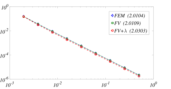
Figure 3: Log-log graphic of FEM and FV $L^{2}$ errors for numerical solutions of Example 1, using $\mathbb{Q}^{1}({\mathcal{T}}_{h})$ discretization, $h=2^{-M}$, $M=1,\dots,9$.

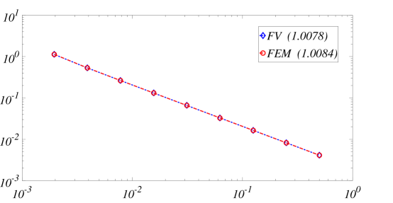
Figure 4: Log-log graphic of FEM and FV $H^{1}$ errors for numerical solutions of Example 1, using $\mathbb{Q}^{1}({\mathcal{T}}_{h})$ discretization, $h=2^{-M}$, $M=1,\dots,9$.

$M$	$FEM,\,\,L^{2}\,Error$	$FV+\lambda,\,L^{2}\,Error$	$FEM,\,\,H^{1}\,Error$	$FV,\,H^{1}\,Error$
$1$	$1.5538\times 10^{-1}$	$1.5103\times 10^{-1}$	$1.1297\times 10^{0}$	$1.1338\times 10^{0}$
$2$	$3.6342\times 10^{-2}$	$3.1881\times 10^{-2}$	$5.3226\times 10^{-1}$	$5.3416\times 10^{-1}$
$3$	$8.9720\times 10^{-3}$	$7.5.276\times 10^{-3}$	$2.6374\times 10^{-1}$	$2.6403\times 10^{-1}$
$4$	$2.2548\times 10^{-3}$	$1.9348\times 10^{-3}$	$1.3163\times 10^{-1}$	$1.3172\times 10^{-1}$
$5$	$5.5513\times 10^{-4}$	$4.6095\times 10^{-4}$	$6.5833\times 10^{-2}$	$6.5840\times 10^{-2}$
$6$	$1.3875\times 10^{-4}$	$1.1513\times 10^{-4}$	$3.2948\times 10^{-2}$	$3.2924\times 10^{-2}$
$7$	$3.4685\times 10^{-5}$	$2.8776\times 10^{-5}$	$1.6418\times 10^{-2}$	$1.6489\times 10^{-2}$
$8$	$8.6711\times 10^{-6}$	$7.1935\times 10^{-6}$	$8.2838\times 10^{-3}$	$8.2141\times 10^{-3}$
$9$	$2.1678\times 10^{-6}$	$1.7983\times 10^{-6}$	$4.1639\times 10^{-3}$	$4.1857\times 10^{-3}$

Table 1: Table of FEM and FV $L^{2}$ and $H^{1}$ errors for numerical solutions of Example 1, using $\mathbb{Q}^{1}({\mathcal{T}}_{h})$ discretization, calculated over $9$ different values of mesh norm, $h=2^{-M}$.

We now consider the case of $\mathbb{Q}^{2}({\mathcal{T}}_{h})$ finite element space. We have computed the FEM solution as well as the solution of the saddle point system (15). We call this last solution the High order FV solution. We estimate the $L^{2}$ and $H^{1}$ errors for both FEM and FV and compare the results through the log-log graphics shown in Figure 5 and Figure 6. See also the Table 2 for comparisons. Numerical convergence is observed with a rate of $2$ for the $H^{1}$ error. The error $p-p^{h}$ is not optimal in $L^{2}$. For this error, the observed convergence rate is close to $2$ but if we observe the error $p-(p^{h}+\lambda^{h})$ in $L^{2}$ we estimate a convergence rate of $3$. These results coincide with our theoretical predictions four our High order FV formulation.

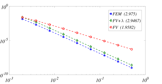
Figure 5: Log-log graphic of FEM and FV $L^{2}$ errors for numerical solutions of Example 1, using $\mathbb{Q}^{2}({\mathcal{T}}_{h})$ discretization, $h=2^{-M}$, $M=1,\dots,9$.

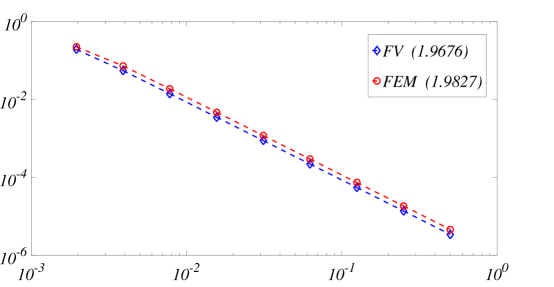
Figure 6: Log-log graphic of FEM and FV $H^{1}$ errors for numerical solutions of Example 1, using $\mathbb{Q}^{2}({\mathcal{T}}_{h})$ discretization, $h=2^{-M}$, $M=1,\dots,9$.

$M$	$FEM\,L^{2}\,Error$	$FV+\lambda,\,L^{2}\,Error$	$FEM\,H^{1}\,Error$	$FV,\,H^{1}\,Error$
$1$	$1.4061\times 10^{-2}$	$2.5448\times 10^{-2}$	$1.9302\times 10^{-1}$	$2.2436\times 10^{-1}$
$2$	$2.1217\times 10^{-3}$	$4.9023\times 10^{-3}$	$5.4862\times 10^{-2}$	$7.2895\times 10^{-2}$
$3$	$2.6860\times 10^{-4}$	$6.4789\times 10^{-4}$	$1.4072\times 10^{-2}$	$1.8847\times 10^{-2}$
$4$	$3.3875\times 10^{-5}$	$8.1756\times 10^{-5}$	$3.5418\times 10^{-3}$	$4.7552\times 10^{-3}$
$5$	$4.2437\times 10^{-6}$	$1.0242\times 10^{-5}$	$8.3539\times 10^{-4}$	$1.2667\times 10^{-3}$
$6$	$5.3075\times 10^{-7}$	$1.2810\times 10^{-6}$	$2.2016\times 10^{-4}$	$2.9616\times 10^{-4}$
$7$	$6.6353\times 10^{-8}$	$1.6015\times 10^{-7}$	$5.5043\times 10^{-5}$	$7.4046\times 10^{-5}$
$8$	$8.2944\times 10^{-9}$	$2.0019\times 10^{-8}$	$1.3761\times 10^{-5}$	$1.8512\times 10^{-5}$
$9$	$1.0369\times 10^{-9}$	$2.5024\times 10^{-9}$	$3.4403\times 10^{-6}$	$4.6280\times 10^{-6}$

Table 2: Table of FEM and FV $L^{2}$ and $H^{1}$ errors for numerical solutions of Example 1, using $\mathbb{Q}^{2}({\mathcal{T}}_{h})$ discretization, calculated over $9$ different values of mesh norm, $h=2^{-M}$.

We now turn our attention to the norm $\|\cdot\|_{V^{h}}$, defined in (37), of the computed error. We introduce the seminorm,

$$|p|_{V^{h}}^{2}=\sum_{\ell=1}^{N_{h}}\left(\|p_{xx}\|_{L^{2}{(R_{\ell})}}^{2}+\|p_{yy}\|_{L^{2}{(R_{\ell})}}^{2}\right)$$ (41)

Note that $\|p\|_{V^{h}}^{2}=|p|_{H^{1}}^{2}+h^{2}|p|_{V^{h}}^{2}$. We present the results in Table 3. We see from this results that the error in the seminorm $|\cdot|_{V^{h}}$ decays linearly with $h$ and recall that this seminorm is scaled by a factor $h$ in the definition of the extended norm $\|\cdot\|_{V^{h}}$ in (37).

$M$	$|p-p^{h}|_{V^{h}}$
$1$	$3.6040\times 10^{0}$
$2$	$1.8127\times 10^{0}$
$3$	$9.0885\times 10^{-1}$
$4$	$4.5506\times 10^{-1}$
$5$	$2.2769\times 10^{-1}$
$6$	$1.1388\times 10^{-1}$
$7$	$5.6954\times 10^{-3}$
$8$	$2.8480\times 10^{-3}$
$9$	$1.4240\times 10^{-3}$

Table 3: Table of scaled seminorm errors, see (41), for FV solution, $h=2^{-M}$. Recall that the seminorm $|\cdot|_{V^{h}}$ in (41) is scaled by a factor $h$ in the definition of the extended norm (37)

.

Using our high order formulation we compute the conservative approximation of the pressure and a Lagrange multiplier which is used to correct the solution for a improved $L^{2}$ approximation. Note that the exact solution value of the Lagrange multiplier is $\lambda=0$. We now compute the error in the Lagrange multiplier approximation in the $M_{h}$ norm. The results are presented in Table 4. We observe a convergence of order $2$ in the approximation of the Lagrange multiplier.

$M$	Error
$1$	$2.4825\times 10^{-1}$
$2$	$9.9023\times 10^{-2}$
$3$	$2.5293\times 10^{-2}$
$4$	$6.3369\times 10^{-3}$
$5$	$1.5848\times 10^{-3}$
$6$	$3.9623\times 10^{-4}$
$7$	$9.9061\times 10^{-5}$
$8$	$2.4765\times 10^{-5}$
$9$	$6.1913\times 10^{-5}$

Table 4: Table of error values $\|\lambda_{h}-\lambda\|_{M_{h}}$ for the Lagrange multiplier approximation.

To finish this subsection we compute energy and conservation of mass indicators in Table 5. The energy is defined as

$$E(p)=\frac{1}{2}\int_{\Omega}|\nabla p|^{2}dx-\int_{\Omega}qp$$ (42)

while the conservation of mass indicator is given by,

$$J(p)=\left(\sum_{R}\left(\int_{\partial R}-\nabla p\cdot\mathbf{n}-\int_{R}q\right)^{2}\right)^{1/2}.$$ (43)

$M$	$\mathbb{Q}^{1},E(u_{FEM})$	$\mathbb{Q}^{2},E(u_{FEM})$	$\mathbb{Q}^{1},E(u_{FV})$	$\mathbb{Q}^{2},E(u_{FV})$
$1$	-4.5230278474	-4.523568683883	-4.5230278425	-4.5233568683864
$M$	$\mathbb{Q}^{1},J(u_{FEM})$	$\mathbb{Q}^{2},J(u_{FEM})$	$\mathbb{Q}^{1},J(u_{FV})$	$\mathbb{Q}^{2},J(u_{FV})$
$1$	$5.2434\times 10^{-6}$	$8.2205\times 10^{-8}$	$2.2928\times 10^{-14}$	$1.0261\times 10^{-13}$

Table 5: Energy minimization and conservation indicator with $h=2^{-9}$.

6.2 Singular forcing with nonhomogeneous Neumann boundary condition

For comparison, we also solve two problems with Neumann boundary conditions. The first problem has a singular forcing term in the form of a font located at $(0,0)$ and a source located in $(1,1)$. The computed solution for this problem is shown in the Figure 7. The second problem has a smooth forcing term.

Table 6 shows $FEM$ and $FV$ computed order of convergence of the error. Apart from computing $L^{1}$ and $L^{2}$ norms of the error we also include the measure of the error in the seminorm $W^{1,1}$ (note that in this case the solution of this problems in not regular and is not in $H^{1}(\Omega)$). We observe here that, in terms of approximation, the performance of both strategies FEM and FV perform similarly with respect to the order of the polynomials. The main difference between the two computed solution is only the conservation of mass that is being satisfied only by the FV solution.

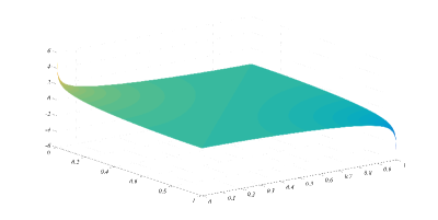
Figure 7: Plot of numerical solution for the problem with homogeneous Neumann boundary conditions and singular right hand side.

$FEM$		$\mathbb{Q}^{1}$	$\mathbb{Q}^{2}$
	$L^{1}$	$1.8463$	$1.8707$
	$L^{2}$	$1.0000$	$1.0121$
	$W^{1,1}$	$0.8694$	$0.9983$
$FV$
$FV+\lambda$	$L^{1}$	$1.8490$	$1.8715$
$FV+\lambda$	$L^{2}$	$1.0000$	$1.0000$
	$W^{1,1}$	$0.8590$	$0.9977$

Table 6: Values of $L^{1}$, $L^{2}$ and $W^{1,1}$ error order of $FEM$ and $FV$ for the homogeneous Neumann boundary condition problem with singular forcing.

6.2.1 Smooth forcing

To finish our comparison with Neumann boundary condition we consider the case where the flux term is given by $q(x,y)=x-y$. In Table 7 we show the results. We obtain expected results with our FV formulation being as accurate as the FEM formulation and still satisfying the conservation of mass restrictions.

$FEM$		$\mathcal{Q}^{1}$	$\mathcal{Q}^{2}$
	$L^{1}$	$1.9999$	$3.0000$
	$L^{2}$	$1.9999$	$3.0000$
	$W^{1,1}$	$1.0000$	$2.0000$
$FV$
$FV+\lambda$	$L^{1}$	$2.0000$	$3.0000$
$FV+\lambda$	$L^{2}$	$1.9999$	$3.0000$
	$W^{1,1}$	$1.0000$	$2.0000$

Table 7: Values of $L^{1}$, $L^{2}$ and $W^{1,1}$ error order of $FEM$ and $FV$ for the homogeneous Neumann boundary condition problem with smooth forcing.

7 Conclusions

In this paper, we introduce a high-order discretization with locally conservative properties for a second-order problem. Our formulation discretizes the second order problem and there is no need to write an equivalent first order system of differential equations. It is, therefore, a novel approach and it is fundamentally different from classical mixed finite element methods such as discretizing by Raviart-Thomas elements. We impose the conservative constraints by using a Lagrange multiplier for each control volume and therefore we can compute locally conservative solutions while keeping the high-order approximation. For the case of constant permeability coefficient, we present the analysis of our formulation at the continuous and discrete levels. In particular, we obtain optimal estimates for the $H^{1}$ and $L^{2}$ norms. We mention also that the optimal $L^{2}$ approximation is obtained without any post-processing or hybridization which are other differences with classical mixed finite element methods. The analysis can be straightforwardly extended to the case of smooth permeability coefficients.

We present numerical experiments that verify our theoretical findings. We also stress the fact that our approximation of the solution has continuous tangential fluxes along primal element edges. The implementation of our method is simple and requires only coding tools used for classical conforming high-order finite element method plus the computation of fluxes of basis functions along control volumes boundaries (as in the classical low-order finite volume method).

Our formulation can be easily extended to a variety of cases where both high-order approximation and also conservative properties are desirable. For instance, we mention the case of flow problems in high-contrast multiscale porous media with sophisticated high-order discretization schemes, see [8]. We note that the analysis for this case and for other high-order approximation spaces is non-trivial as well as robust solvers are under investigation.

Acknowledgement:
Eduardo Abreu thanks in part by FAPESP 2016/23374-1 and CNPq Universal 445758/2014-7. Ciro Diaz thanks CAPES for a graduate fellowship. Marcus Sarkis thanks in part by NSF-MRI 1337943 and NSF-MPS 1522663.