Mid-infrared extinction and fresh silicate dust towards the Galactic Center

Abstract

We interpret the interstellar extinction observed towards the Galactic Center (GC) in the wavelength range $\lambda=1-20\,\mu{\rm m}$. Its main feature is the flat extinction at $3-8\,\mu{\rm m}$ whose explanation is still a problem for the cosmic dust models. We search for structure and chemical composition of dust grains that could explain the observed extinction. In contrast to earlier works we use laboratory measured optical constants and consider particles of different structure. We show that a mixture of compact grains of aromatic carbon and of some silicate is better suited for reproducing the flat extinction in comparison with essentially porous grains or aliphatic carbon particles. Metallic iron should be located inside the particle, i.e. cannot form layers on silicate grains as the extinction curves become then very peculiar. We find a model including aromatic carbonaceous particles and three-layered particles with an olivine-type silicate core, a thin very porous layer and a thin envelope of magnetite that provides a good (but still not perfect) fit to the observational data. We suggest that such silicate dust should be fresh, i.e. recently formed in the atmospheres of late-type stars in the central region of the Galaxy. We assume that this region has a radius of about 1 kpc and produces about a half of the observed extinction. The remaining part of extinction is caused by a “foreground” material being practically transparent at $\lambda=4-8\,\mu{\rm m}$.

=5

1 Introduction

The center parts of the Milky Way are a unique place to study different processes in the vicinity of a supermassive black hole as well as dynamics and star formation under extreme conditions (Genzel et al., 2010; Mapelli & Gualandris, 2016). The Galactic Center (GC) invisible at the optical wavelengths can be observed in the infrared (IR) where the extinction amounts to $A_{\rm Ks}=2\fm 49$ (Fritz et al., 2011). A distinguishing feature of the GC extinction is its flat wavelength dependence at $3\,\mu{\rm m}<\lambda<8\,\mu{\rm m}$. The flat or gray extinction in the GC was firstly measured by Lutz et al. (1996) with ISO, using hydrogen recombination lines, and confirmed by Lutz (1999), Nishiyama et al. (2009), and Fritz et al. (2011). Numerous recent observations appear to suggest the universality of flat extinction in the mid-IR for both diffuse and dense environments (see Wang et al., 2013,  for a summary).

Fritz et al. (2011) have compared different dust models capable of explaining the mid-IR extinction in the GC. The models were from Weingartner & Draine (2001) (mixture of carbonaceous and silicate spheres), Zubko et al. (2004) (mixture of carbonaceous and silicate particles and additionally composite grains consisting of silicates, organic refractory material, water ice, and voids), Dwek (2004) (mixture of bare particles of Zubko et al. (2004) and additionally metallic needles), and Voshchinnikov et al. (2006) (multi-layered spheres consisting of silicate, carbon, and vacuum). Wang et al. (2014) have developed the idea of Dwek (2004) and considered additionally micrometer-sized particles from amorphous carbon, graphite, silicate or iron. Such a model with amorphous carbon explained the flat extinction at $3-8\,\mu{\rm m}$, but required the solid-phase C abundance C/H$=$352 ppm that exceeded the solar abundance of carbon (269 ppm, Asplund et al., 2009). An important feature of the modelings mentioned above is a priori selection of the optical constants of grain materials. Moreover, all the authors used the optical constants of the “astronomical silicate” (astrosil) obtained by empirical fits to some observations by Draine & Lee (1984). The imaginary part of the complex refractive index of astrosil $k$ slightly grows with $\lambda$ in the region $3-8\,\mu{\rm m}$, which does not coincide with the behaviour of $k$ for any silicate material (see Fig. A.1 in Jones et al., 2013).

It should be emphasized that there are no cosmic dust models that can explain the flat (excess) mid-IR extinction observed in the GC and other galactic objects. The COMP-AC-S model of Zubko et al. (2004) gives a good fit, but produces strong 3 $\mu{\rm m}$ band, which disagrees with the trend found in the Coalsack nebula Globule 7 by Wang et al. (2013). The most recent model of Wang et al. (2015) includes $4\,\mu{\rm m}$ clean water ice particles and does explain both mid-IR extinction and the abundance of oxygen in dust, but the ice particles hardly can be so large and clean in the interstellar medium (ISM).

In this paper, we analyze a large set of dust models, concentrating on variations of grain structure and a proper presentation of grains’ chemical composition, to find a model that fits the near- and mid-IR extinctions and the 10 $\mu{\rm m}$ feature observed to the GC. The next section contains a description of the observational data and the models. The results and their discussion are presented in Sect. 3. Concluding remarks are given in Sect. 4.

2 Observational data and dust model

The GC extinction has been observationally obtained by Fritz et al. (2011) (the region 1.3–19 $\mu{\rm m}$), Nishiyama et al. (2009) (1.2–8 $\mu{\rm m}$), and Chiar & Tielens (2006) (1.2–25 $\mu{\rm m}$). The latter paper contains the probable extinction profile of the 9.7 $\mu{\rm m}$ silicate feature for the GC. All data have been normalized by us in order to have $A_{\rm Ks}=2\fm 49$ at $\lambda_{\rm Ks}=2.17\,\mu{\rm m}$,

$$A^{*}(\lambda)=\frac{A(\lambda)}{A_{\rm Ks}}\,2\fm 49\,.$$ (1)

They are plotted in all Figures below.

It should be note that the GC extinction was estimated from observations in different ways. As a result, the data of Fritz et al. (2011) were mainly derived for the central 14${}^{\prime\prime}\times$20^′′ region, the data of Nishiyama et al. (2009) are averaged over the region $|l|<3^{\circ},|b|<1^{\circ}$, and the data of Chiar & Tielens (2006) are the extinction towards the Wolf-Rayet star WR 98a ($l\approx 358^{\circ},b\approx 0^{\circ}$) extended to the line of sight to GCS3. However, the extinction law for $\lambda<14\,\mu{\rm m}$ is practically the same. Hence, the data can be combined, and the question on where is located the dust that produces the extinction is not as important as it could be.

We base our analysis on the model of Hirashita & Voshchinnikov (2014) who chose the initial size distributions of silicate and carbonaceous dust that fited the mean Milky Way extinction curve with $R_{V}=3.1$ (Weingartner & Draine, 2001) and considered dust grain size evolution due to the accretion and coagulation processes.

So, our model contains two populations of grains: silicate (Si) and carbonaceous (C) ones with the size distributions from Hirashita & Voshchinnikov (2014). As extinction only weekly depends on the particle shape (Voshchinnikov & Das, 2008), we assume that dust grains are spherical.

Thus, the model has the following parameters: 1) the chemical composition of silicate and carbonaceous particles; 2) the structure of particles; 3) the relative number of silicate grains ${\cal K}_{\rm Si}=N_{\rm Si}/N_{\rm dust}$, where $N_{\rm Si}$ and $N_{\rm dust}$ are the column densities of silicate grains and all dust particles, respectively; 4) the time of evolution. Sometimes, we also included an additional population of dust.

When considering the chemical composition, we mainly oriented on the optical constants obtained in Jena laboratory (http://www.astro-uni-jena.de/Laboratory/). Information about these and many other data is collected in the Heidelberg–Jena–Petersburg Database of Optical Constants (HJPDOC) described by Henning et al. (1999) and Jäger et al. (2003b). The materials used for our modelling are outlined in Table 4 in the Appendix.

For homogeneous spheres, the extinction efficiency factors were calculated with the Mie theory. For composite particles, the factors were computed by using the Mie theory and the Bruggeman mixing rule of the EMT or the theory for multi-layered spheres (see Voshchinnikov & Mathis, 1999).

3 Results and discussion

Table 2: Best-fit dust models

$N$	Model components	$\chi^{2}$/d.o.f.	$A^{*}(7.5\,\mu{\rm m})$	$R_{V}$	$\lambda_{m}$	$A^{*}(\lambda_{m})$	Figs.
	Observations	–	0.81	$\lesssim 3$:	9.6	3.45	Figs. 1–4
Homogeneous spheres
1	astrosil (${\cal K}_{\rm Si}=0.50$) / ACBE$\_$zu	36.4	0.561	3.07	9.5	3.43	Fig. 1
2	olmg50 (${\cal K}_{\rm Si}=0.25$) / cell400	116.4	0.320	3.25	9.8	3.41	Fig. 1
3	olmg50 (${\cal K}_{\rm Si}=0.55$) / cell1000	36.6	0.321	3.26	9.8	3.36	Fig. 1
4	olmg40 (${\cal K}_{\rm Si}=0.77$) / cell1000	112.9	0.261	3.29	9.8	3.46
5	olmg100 (${\cal K}_{\rm Si}=0.56$) / cell1000	36.1	0.706	2.61	9.7	3.46
6	pyrmg50 (${\cal K}_{\rm Si}=0.47$) / cell1000	47.8	0.381	2.87	9.2	3.47	Fig. 1
7	pyrmg40 (${\cal K}_{\rm Si}=0.48$) / cell1000	43.1	0.386	3.00	9.0	3.49
8	pyrmg100 (${\cal K}_{\rm Si}=0.39$) / cell1000	74.9	0.385	2.73	9.4	3.48
9	OHM-SiO (${\cal K}_{\rm Si}=0.92$) / cell1000	35.4	0.503	4.02	10.0	3.41
10	olmg50 (${\cal K}_{\rm Si}=0.44$) / H2O (${\cal K}_{\rm H_{2}O}=0.20$) / cell1000	30.4	0.420	2.98	9.8	3.42
11	olmg50 (${\cal K}_{\rm Si}=0.50$) / Fe (${\cal K}_{\rm Fe}=0.20$) / cell1000	87.8	0.208	3.94	9.8	1.84
EMT-Mie calculations
12	80%olmg50+20% vac (${\cal K}_{\rm Si}=0.53$) / cell1000	32.9	0.338	2.64	10.0	2.86
13	olmg50 (${\cal K}_{\rm Si}=0.46$) / 80%cell1000+20% vac	26.4	0.383	3.34	9.8	2.78
14	a-SilFe (${\cal K}_{\rm Si}=0.40$) / cell1000	37.2	0.312	4.60	9.9	1.40
15	a-SilFe (${\cal K}_{\rm Si}=0.34$) / optEC(s)	487.0	0.080	3.92	10.0	3.41
16	amFo-10Fe30FeS (${\cal K}_{\rm Si}=0.47$) / cell1000	40.6	0.287	4.29	9.9	1.64
17	amEn-10Fe30FeS (${\cal K}_{\rm Si}=0.39$) / cell1000	36.5	0.290	5.06	9.5	1.77
Core-mantle spheres
18	20% vac–80% olmg50 (${\cal K}_{\rm Si}=0.53$) / cell1000	32.6	0.335	2.66	10.0	2.82
19	olmg50 (${\cal K}_{\rm Si}=0.44$) / 20% vac–80%cell1000	25.9	0.380	3.68	9.8	2.53
20	93% a-SilFe–7% cel1000 (${\cal K}=0.28$) / 73% optEC(s)–27% cell1000	313.9	0.240	3.48	10.0	3.44	Fig. 4
21	93% olmg50–7% cel1000 (${\cal K}=0.19$) / 73% cel400–27% cell1000	90.1	0.391	2.99	9.8	3.35
Three-layered spheres
22	10% Fe–10% vac∗–80% olmg50 (${\cal K}=0.77$) / cell1000	164.3	0.231	3.06	9.8	3.41	Fig. 2
23	10% vac–10% Fe–80% olmg50 (${\cal K}=0.18$) / cell1000	68.5	0.280	5.29	9.6	0.68	Fig. 2
24	98.99% olmg50–1% vac∗–0.01% Fe (${\cal K}=0.09$) / cell1000	89.5	1.213	4.83	8.2	1.49	Fig. 2
25	90% olmg50–5% vac∗–5% Fe3O4 (${\cal K}=0.91$) / cell1000	6.7	0.696	3.22	9.8	3.45	Fig. 3, 4
26	90% olmg50–5% vac∗–5% Fe2O3 (${\cal K}=0.47$) / cell1000	31.7	0.332	3.56	9.8	2.39	Fig. 3
27	90% olmg50–5% vac∗–5% FeO (${\cal K}=0.48$) / cell1000	36.2	0.319	3.51	9.8	2.21	Fig. 3
28	90% olmg50–5% vac∗–5% FeS (${\cal K}=0.16$) / cell1000	94.3	0.319	4.42	9.8	0.61	Fig. 3
29	90% pyrmg50–5% vac∗–5% Fe3O4 (${\cal K}=0.72$) / cell1000	75.7	0.781	2.91	9.1	3.22
Two-cloud model
30	model 20 + model 25 (see Sect. 3.4)	84.9	0.468	3.32	9.9	3.41	Fig. 4

NOTES. Column 3: fit goodness $\chi^{2}$/d.o.f., where d.o.f. means the degree of freedom (we took it equal to 24); Column 4: normalized extinction at $\lambda=7.5\,\mu{\rm m}$; Column 5: ratio of the total-to-selective extinction; Column 6: position of the 10 $\mu{\rm m}$ peak in $\mu{\rm m}$; Column 7: normalized strength of the 10 $\mu{\rm m}$ peak; vac^∗ — very porous layer.

We varied the model parameters to fit the observed GC extinction. The number of possible model variants is very large, but it can be significantly reduced by applying available knowledge on the physics of dust formation, growth and evolution (see, e.g., Chiar et al., 2013; Jones et al., 2013; Gail & Sedlmayr, 2014).

Information about some models considered is collected in Table 3 which gives a description of the model (column 2), normalized $\chi^{2}$ characterizing the goodness of the fit for 29 observational points from Fritz et al. (2011) and Nishiyama et al. (2009) (column 3), obtained values of normalized extinction at $\lambda=7.5\,\mu{\rm m}$ $A^{*}(7.5\,\mu{\rm m})$ (assuming $A_{\rm Ks}=2\fm 49$, column 4), $R_{V}$ (ratio of the total-to-selective extinction, column 5) and the position and strength of the 10 $\mu{\rm m}$ peak (columns 6 and 7).

The fitting procedure was as follows. First, we fitted the extinction shortward 8.8 $\mu{\rm m}$, i.e. 19 points from Fritz et al. (2011) and all 10 points from Nishiyama et al. (2009). The values of the normalized $\chi^{2}$ given in Table 3 just characterize this fitting. Then, by varying the fraction of silicate grains ${\cal K}_{\rm Si}$, we fitted the relative strength of the 10 $\mu{\rm m}$ band. The position of the band was mainly fitted by the proper choice of the silicate material. The relative strength and position of the band at 10 $\mu{\rm m}$ were taken from Chiar & Tielens (2006). Note that their data for the 18 $\mu{\rm m}$ band are less reliable and that many silicates have the bending bands in the range $16-23\,\mu{\rm m}$ (see Henning, 2010). Therefore, we did not model the 18 $\mu{\rm m}$ band.

3.1 Homogeneous particles

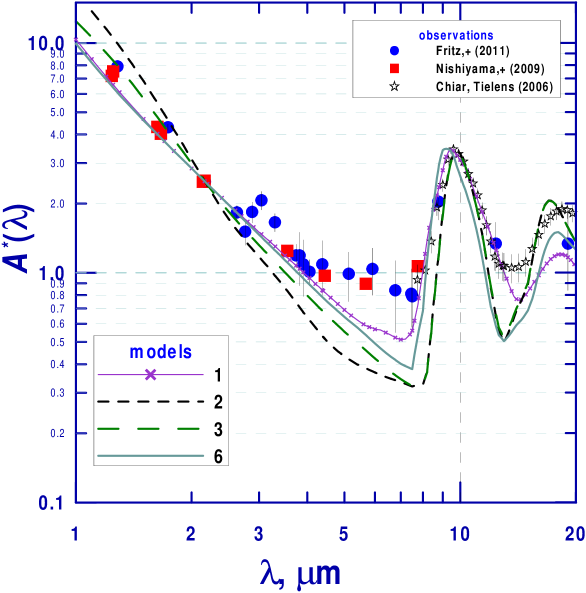
Figure 1: Comparison of the normalized IR extinction observed towards the Galactic Center with that predicted by the models with homogeneous particles. The model numbers are from Table 3.

We have considered a number of two- and three-component models with compact homogeneous grains. We started with the standard mixture of grains of artificial silicate, astrosil, and amorphous carbon ACBE$\_$zu (model 1, see Table 3 and Fig. 1). As expected, the wavelength dependence of extinction derived was steeper than that given by observations.

The next step was to find better models by variations of the laboratory optical constants. A comparison between the models with the aliphatic and aromatic carbon (models 2, 3) showed that the near-IR ($\lambda<2\,\mu{\rm m}$) and mid-IR extinction was much better reproduced by the model with aromatic carbon cell1000. So, we chose this material as the basic one in the subsequent modelling.

Note that the carbon materials cell400 and cell1000 used by us differ in the degree of “graphitization” (Jäger et al., 1998). Therefore, for the former, in first approximation the imaginary part of the refractive index $k\sim\lambda^{-1}$ for $\lambda=1-10\,\mu{\rm m}$, while for the latter, $k\approx{\rm const.}$ (for graphite, $n,k$ grow with $\lambda$). Obviously, such graphitization favours excess IR extinction.

Further, we examined different types of silicates: olivines and pyroxenes with different content of Mg and Fe (models 3 – 8). As can be seen, olivines better explain the observations as the silicate peak produced by pyroxenes is shifted to $\lambda=9.0-9.4\,\mu{\rm m}$ (Table 3 and Fig. 1). Though forsterite grains (model 5) well fit the observed mid-IR extinction, in this case dust grains contain no iron, which is hardly probable according to contemporary understanding of cosmic dust origin and evolution. Our attempts to add iron or water ice as the third component into our silicate-carbonaceous mixture (models 10, 11) failed as mid-IR extinction always became steeper.

3.2 EMT-Mie calculations and core-mantle particles

The physical conditions in which dust grains originate and grow should lead to formation of heterogeneous particles, in particular, porous. Two grain structures are generally expected: layered particles corresponding to subsequent accretion of different species, and an alternative — particles with small more or less randomly distributed inclusions. In the former case the optical properties of heterogeneous particles are modelled with the Mie-like theory for layered particles (in particular, core-mantle), in the latter case by using homogeneous particles with the averaged dielectric functions (EMT-Mie calculations).

We present four models with porous silicate or carbonaceous particles (models 12, 13 and 18, 19) to illustrate that the porosity does not make the fitting much better in a comparison with compact grains, but leads to the shift and decrease of the silicate peak.

We have also considered the models with the refractive indexes constructed by Jones (2012), Jones et al. (2013) and Köhler et al. (2014) (models 14 – 17). None of these models produces the flat mid-IR extinction with the worst fit to the data given by aliphatic carbon optEC_(s) (model 15). The models 20 and 21 with core-mantle grains give a good opportunity to test the hypotheses of Jones et al. (2013) who predicted that in the diffuse ISM large a-C:H grains are to be covered by a a-C 20 nm thick envelope and large Si grains by a a-C 5 nm thick envelope. As can be seen, in this case extinction is inconsistent with the observations of the flat mid-IR extinction in the GC.

Note that an increase of the thickness of the a-C mantles of silicate grains leads to an increase of the mid-IR extinction as has been demonstrated in the work of Köhler et al. (2014), where they have also analyzed the effect of “dirtiness” of silicates (due to absorbing inclusions of FeS). However, this increase is certainly not enough, while the thick a-C mantles begin to affect the silicate bands strength (see their Fig. 3).

3.3 Three-layered particles

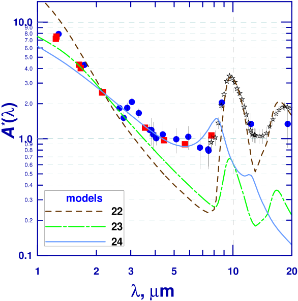
Figure 2: Same as Fig. 1 but for the models with mixtures of the three-layered silicate particles and homogeneous carbonaceous particles. Three-layered particles consist of olivine, iron and vacuum. Fe is located in the particle core (model 22), intermediate layer (model 23) or outer layer (model 24).

The use of multi-layered particles permits a more sophisticated treatment of the processes of grain growth and evolution. Specifically, it is possible to analyse the role of iron which is one of the major dust-forming elements (Jones, 2000; Dwek, 2016). The abundance of iron in the solid-phase of the ISM may reach 97 – 99% of the cosmic abundance (Voshchinnikov & Henning, 2010). Iron can be incorporated into dust grains in the form of oxides (FeO, Fe₂O₃, Fe₃O₄), (Mg/Fe)-silicates, sulfide (FeS), and metallic iron. The last two cases come from the contemporary theory of dust condensation in circumstellar environments. Gail & Sedlmayr (1999, 2014) note that Fe and FeS start to condense at temperatures well below the stability limits of silicates like forsterite and enstatite. This should lead to formation of layered particle. At low temperatures, the conversion of solid iron into iron oxides may occur (Gail & Sedlmayr, 2014, p. 306).

Figure 2 shows the wavelength dependence of extinction for the models with three-layered particles including of olivine and vacuum. Iron is located in the particle core (model 22), intermediate layer (model 23), or outer layer (model 24). As seen, the presence of metallic iron at any place inside a particle, excluding its core, drastically changes extinction — iron totally screens the underlying layers and influences the optics of the overlying ones. As a result, one cannot properly reproduce either the position and shape of the observed silicate band (models 23, 24) or the slope of the wavelength dependence of IR extinction (models 22, 23).

However, iron can be oxidized or sulfidized, which opens a way to explain the observations. Figure 3 shows the extinction calculated for four models with olivine particles (olmg50) coated by a thin very porous layer and a thin (2 – 3 nm thick) envelope of iron oxide or iron sulfide. It is evident that the model 25 with magnetite agrees closely with the observational data. This model well reproduces near-IR extinction and the 10 $\mu{\rm m}$ peak and gives nearly as large mid-IR extinction as observed. The model also produces the visual extinction $A_{V}/A_{Ks}=15.2$ which is close to the observed median value equal to $13.4$ (Nataf et al., 2016).

Note that the replacement of olivine with pyroxene (model 29) leads to even a better coincidence with the observed extinction at $\lambda=5-9\,\mu{\rm m}$ but does not allow one to explain properly the near-IR extinction and the position of the silicate feature.

So, we see that the model 25 is practically the only way of successful fitting of the data, when keeping in mind available information on cosmic dust. Considering the model 25 with the particles from olivine olmg50 and amorphous carbon cell1000 as a prototype of possible dust models for the GC.

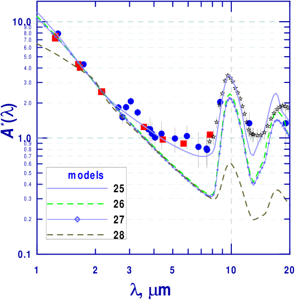
Figure 3: Same as Fig. 2 but for three-layered particles consisting of olivine (core), very porous intermediate layer and iron oxide or sulfide (outer layer). The outer layer is from Fe₃O₄ (model 25), Fe₂O₃ (model 26), FeO (model 27) or FeS (model 28).

3.4 Foreground extinction

In previous modelling we ignored the distribution of the extinction along the line of sight. However, the 3-dimensional extinction map of the GC shows that about half of the extinction in the sightlines of Nishiyama et al. (2009) is reached in a distance of about 5 kpc from the Sun (see Fig. 9 in Schultheis et al., 2014).

We assume different populations of dust grains in the foreground dusty complexes and in the central galactic region Most likely the dust producing the foreground extinction is processed, in particular, the silicate grains are covered by carbon (Jones et al., 2013). Such grains are properly described by the theoretical model 20 and give very low relative extinction in the mid-IR ($A(7.5\,\mu{\rm m})/A_{\rm Ks}\sim 0.1-0.2$, see Fig. 4 and Köhler et al., 2014). However, there exist several places in the Galaxy where low mid-IR extinction has been observed. On Fig. 4 we plotted the average extinction for three molecular clouds obtained by Chapman et al. (2009). It is visible that the model 20 agrees roughly with the measurements.

For the central galactic region, we applied the model 25 with freshly formed silicate dust. The total extinction for our “two-cloud” model was calculated as

$$A_{\rm total}^{*}(\lambda)=f\,A^{*}_{\rm foregr}(\lambda)+(1-f)\,A^{*}_{\rm backgr}(\lambda),$$ (2)

where $f$ is the contribution of the foreground clouds to the total extinction. At the moment, the available data (see, e.g., Schultheis et al., 2014) do not allow one to estimate the value of $f$ with a sufficient accuracy, therefore, we just use 0.5 for simplicity.

Figure 4 and Table 3 show the extinction produced by the two-cloud model ($f=0.5$). Its agreement with the observational data is not perfect but good enough.

4 Concluding remarks

According to the modern ideas on cosmic dust evolution in the diffuse ISM, the silicate grains should be covered by a significant envelope from amorphous carbon on a short time scale (Jones et al., 2013). Moreover, amorphous olivine MgFeSiO₄ (olmg50) is a possible mineral in dust grains forming in the atmospheres of late-type giants, but it is not believed to be the main material of silicate particles in the ISM (see, e.g., Jäger et al., 2003b). Therefore, we suggest that silicate dust in our model is “fresh”, i.e. recently formed in the atmospheres of the late-type stars in the GC. Our suggestion is rather natural as the GC is dominated by old stars.

Carbonaceous particles are more processed in comparison with silicate ones that is determined by lower efficiency of their destruction (Slavin et al., 2015). Intense radiation fields in the GC are favourable for the fast photo–dissociative aromatisation of a-C(:H) materials (Jones et al., 2013, 2014).

Obviously, the model found by us does not fit the data perfectly and one cannot exclude other possible solutions to the problem of the flat mid-IR extinction towards the GC. However, we pay attention to the potential of our approach — to relate the problem solution with specific structure and composition of dust grains relying the laboratory data on optical constants and contemporary ideas on cosmic dust grain evolution.

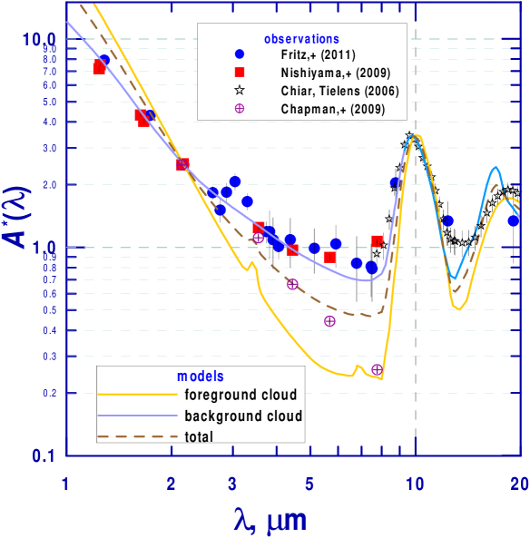
Figure 4: Comparison of the normalized IR extinction observed towards the Galactic Center (filled circles and squares) with that predicted by the model 20 with processed core-mantle particles in the foreground cloud and model 25 with fresh silicate 3-layered particles in the background cloud. Dashed brown line shows the total extinction produced in the foreground and background clouds as calculated from Equation (2). Crossed circles present the average wavelength dependence of the interstellar extinction for three molecular clouds in the local ISM (Chapman et al., 2009).

Table 3: Sources of optical constants

Notation	Material	Reference
astrosil	astronomical silicate	Draine (2003)
olmg50	amorphous olivine (MgFeSiO4)	Dorschner et al. (1995)
olmg40	amorphous olivine (Mg0.8Fe1.2SiO4)	Dorschner et al. (1995)
olmg100	amorphous olivine (Mg2SiO4, forsterite)	Jäger et al. (2003a)
pyrmg50	amorphous pyroxene (Mg0.5Fe0.5SiO3)	Dorschner et al. (1995)
pyrmg40	amorphous pyroxene (Mg0.4Fe0.6SiO3)	Dorschner et al. (1995)
pyrmg100	amorphous pyroxene (MgSiO3, enstatite)	Dorschner et al. (1995)
OHM-SiO	O-rich interstellar silicate	Ossenkopf et al. (1992)
a-SilFe	amorphous olivine (MgFeSiO4+10%Fe)	Jones et al. (2013)
amFo-10Fe30FeS	amorphous forsterite (Mg2SiO4+10%Fe+30%FeS)	Köhler et al. (2014)
amEn-10Fe30FeS	amorphous enstatite (MgSiO3+10%Fe+30%FeS)	Köhler et al. (2014)
ACBE$\_$zu	amorphous carbon (type BE)	Zubko et al. (1996)
cell400	pyrolizing cellulose ($T=400\arcdeg$C, aliphatic, a-C(:H))	Jäger et al. (1998)
cell1000	pyrolizing cellulose ($T=1000\arcdeg$C, aromatic, a-C)	Jäger et al. (1998)
optEC(s)	amorphous carbon (a-C(:H), band gap $E_{g}=2.5$ eV)	Jones (2012)
Fe	iron	Jones et al. (2013)
FeO	wüstite	Henning et al. (1995)
Fe2O3	hematite	Jena laboratory
Fe3O4	magnetite	Jena laboratory
FeS	troilite	Pollack et al. (1994)
H2O	water ice	Warren & Brandt (2008)

References

- Asplund et al. (2009) Asplund, M., Grevesse, N., Sauval, A. J., & Scott, P. 2009, ARA&A, 47, 481
- Chiar & Tielens (2006) Chiar, J. E., & Tielens, A. G. G. M. 2006, ApJ, 637, 774
- Chapman et al. (2009) Chapman, N. L., Mundy, L. G., Lai, S.-P., & Evans II, N. J. 2009, ApJ, 690, 496
- Chiar et al. (2013) Chiar, J. E., Tielens, A. G. G. M., Adamson, A. J., & Ricca, A. 2013, ApJ, 770, 78
- Das et al. (2010) Das, H. K., Voshchinnikov, N. V., & Il’in, V. B. 2010, MNRAS, 404, 265
- Dorschner et al. (1995) Dorschner, J., Begemann, B., Henning, Th., et al. 1995, A&A, 300, 503
- Draine (2003) Draine, B. T. 2003, ApJ, 598, 1026
- Draine & Lee (1984) Draine, B. T., & Lee, H. M. 1984, ApJ, 285, 89
- Dwek (2004) Dwek, E. 2004, ApJ, 611, L109
- Dwek (2016) Dwek, E. 2016, ApJ, 825, 136
- Fritz et al. (2011) Fritz, T. K., Gillessen, S., Dodds-Eden, K., et al. 2011, ApJ, 737, 73
- Gail & Sedlmayr (1999) Gail, H.-P., & Sedlmayr, E. 1999, A&A, 347, 594
- Gail & Sedlmayr (2014) Gail, H.-P., & Sedlmayr, E. 2014, Physics and Chemistry of Circumstellar Dust Shells (New York, Cambridge University Press)
- Gao et al. (2013) Gao, J., Li, A., & Jiang, B. W. 2013, EP&S, 65, 1127
- Genzel et al. (2010) Genzel, R., Elsenhauer, F., & Gillessen, S. 2010, RvMP, 82, 3121
- Henning (2010) Henning, Th. 2010, ARA&A, 48, 21
- Henning et al. (1995) Henning, Th., Begemann, B., Mutschke, H., & Dorschner, J. 1995, A&AS, 112, 143
- Henning et al. (1999) Henning, Th., Il’in, V. B., Krivova, N. A., et al. 1999, A&AS, 136, 405
- Hirashita & Voshchinnikov (2014) Hirashita H., & Voshchinnikov N. V. 2014, MNRAS, 437, 1636
- Jäger et al. (1998) Jäger, C., Mutschke, H., & Henning, Th. 1998, A&A, 332, 291
- Jäger et al. (2003a) Jäger, C., Dorschner, J., Mutschke, H., et al. 2003a, A&A, 408, 193
- Jäger et al. (2003b) Jäger, C., Il’in, V. B., Henning, Th., et al. 2003b, J. Quant. Spec. Radiat. Transf., 79–80, 765
- Jones (2000) Jones A. P. 2000, JGR, 105, 10257
- Jones (2012) Jones A. P. 2012, A&A, 540, A2 (corrigendum 2012, A&A, 545, C2)
- Jones et al. (2013) Jones, A. P., Fanciullo, L., Köhler, M., et al. 2013, A&A, 558, A62
- Jones et al. (2014) Jones, A. P., Ysard, N., Köhler M., et al. 2014, FaDi, 168, 313
- Köhler et al. (2014) Köhler, M., Jones, A., & Ysard, N. 2014, A&A, 565, L9
- Lutz (1999) Lutz, D. 1999, In The Universe as seen by ISO, ed. P. Cox & M. F. Kessler (1999ESASP 427; Noordwijk: ESA), 623
- Lutz et al. (1996) Lutz, D., Feuchtgruber, H., Genzel, R., et al. 1996, A&A, 315, L269
- Mapelli & Gualandris (2016) Mapelli, M., & Gualandris, A. 2016, LNP, 905, 205
- Mathis et al. (1977) Mathis, J. S., Rumpl, W., & Nordsiek, K. H. 1977, ApJ, 217, 425
- Nataf et al. (2016) Nataf, D. M., Gonzalez, O. A., Casagrande, L., et al. 2016, MNRAS, 456, 2692
- Nishiyama et al. (2009) Nishiyama, S., Tamura, M., Hatano, H., et al. 2009, ApJ, 696, 1407
- Ossenkopf et al. (1992) Ossenkopf, V., Henning, Th., & Mathis, J. S. 1992, A&A, 261, 567
- Pollack et al. (1994) Pollack, J. B., Hollenbach, D., Beckwith, S., et al. 1994, ApJ, 421, 615
- Schultheis et al. (2014) Schultheis, M., Chen, B. Q., Jiang, B. W., et al. 2014, A&A, 566, A120
- Slavin et al. (2015) Slavin, J. D., Dwek, E., & Jones, A. P., 2015, ApJ, 803, 7
- Voshchinnikov (2012) Voshchinnikov, N. V. 2012, J. Quant. Spec. Radiat. Transf., 113, 2334
- Voshchinnikov & Das (2008) Voshchinnikov, N. V., & Das, H. K. 2008, J. Quant. Spec. Radiat. Transf., 109, 1527
- Voshchinnikov & Henning (2010) Voshchinnikov, N. V., & Henning, Th. 2010, A&A, 517, A45
- Voshchinnikov & Mathis (1999) Voshchinnikov, N. V., & Mathis, J. S. 1999, ApJ, 526, 257
- Voshchinnikov et al. (2006) Voshchinnikov, N. V., Il’in, V. B., Henning, Th., & Dubkova, D. N. 2006, A&A, 445, 167
- Wang et al. (2013) Wang, S., Gao, J., Jiang, B. W., et al. 2013, ApJ, 773, 30
- Wang et al. (2014) Wang, S., Li, A., & Jiang, B. W. 2014, P&SS, 100, 32
- Wang et al. (2015) Wang, S., Li, A., & Jiang, B. W. 2015, MNRAS, 454, 569
- Warren & Brandt (2008) Warren, S. G. & Brandt, R. E. 2008, JGR, 113, D14220
- Weingartner & Draine (2001) Weingartner, J. C., & Draine, B. T. 2001, ApJ, 548, 296
- Zubko et al. (1996) Zubko, V. G., Mennella, V., Colangeli, L., et al. 1996, MNRAS, 282, 1321
- Zubko et al. (2004) Zubko, V., Dwek, E., & Arendt, R. G. 2004, ApJS, 152, 211