Charged hydrophobic colloids at an oil/aqueous phase interface

Abstract

Hydrophobic PMMA colloidal particles, when dispersed in oil with a relatively high dielectric constant, can become highly charged. In the presence of an interface with a conducting aqueous phase, image charge effects lead to strong binding of colloidal particles to the interface, even though the particles are wetted very little by the aqueous phase. In this paper, we study both the behavior of individual colloidal particles as they approach the interface, and the interactions between particles that are already interfacially bound. We demonstrate that using particles which are minimally wetted by the aqueous phase allows us to isolate and study those interactions which are due solely to charging of the particle surface in oil. Finally, we show that these interactions can be understood by a simple image-charge model in which the particle charge $q$ is the sole fitting parameter.

I Introduction

Understanding the behavior of colloidal particles at fluid interfaces is a long-standing Ramsden (1903) and actively studied problem in soft condensed matter physics Frydel et al. (2007); Oettel and Dietrich (2008); Cui et al. (2013); Poulichet and Garbin (2015). Extensive experimental and theoretical work has been carried out on interactions between particles that are partially wetted by both fluids, that is, systems where the equilibrium contact angle $\theta_{C}$ falls in the range $0^{\circ}<\theta_{C}<180^{\circ}$. As noted by Pieranski Pieranski (1980), the presence of a fluid interface can lead to a charge asymmetry in the vicinity of each wetted particle, and hence to interactions which are dipolar in form. Indeed, the $r^{-4}$ force law characteristic of dipole-dipole repulsion has been observed in many experiments Aveyard et al. (2002); Park et al. (2014); Parolini et al. (2015).

However, various aspects of the interactions between interfacial particles are still not well-understood McGorty et al. (2010). For instance, interfacial colloids may form repulsive crystals or fractal aggregates Reynaert et al. (2006), or may self-assemble into more complex mesoscopic structures Ghezzi and Earnshaw (1997). The interactions responsible for this collective behavior are typically very sensitive to the protocol used to prepare the samples Park and Furst (2011); Gao et al. (2014), are highly non-uniform Park et al. (2010), and are strongly time-dependent Gao et al. (2014).

Figure 1: (Color online) (A) Once bound to the interface, non-wetting colloids repel electrostatically. (B) Optical micrographs of a single run of an experiment to probe the repulsive force between pairs of interfacial colloids, each with a diameter $d=$1.1\text{\,}\mathrm{\SIUnitSymbolMicro m}$$. (i) & (ii) Two interfacial particles, more than $20\text{\,}\mathrm{\SIUnitSymbolMicro m}$ away from any others, are identified using a particle tracking algorithm, and (iii) automatically dragged to a pre-assigned location using laser tweezers. (iv) The particles are released from the tweezers, and move freely along the interface. Their trajectores (shown in red) are recorded throughout.

To explain these complicated interactions, different authors have proposed various modifications or extensions of Pieranski’s simple model. These include mechanisms for interparticle attraction, such as from inhomogenous charge distribution on the particle surface Chen et al. (2009), and interparticle repulsion, for example by charging of the particle surface in oil Aveyard et al. (1999); Gao et al. (2014). Finite-ion-size effects in the aqueous phase have been proposed to explain the anomalous dependence of the interparticle force on salt concentration Masschaele et al. (2010), while irregular pinning of the contact line on the colloid surface introduces anisotropic capillary forces between particles Stamou et al. (2000); Kaz et al. (2011). Moreover, since all these effects can in principle occur at the same time in the same sample, it is difficult to disentangle them.

In this paper, we report measurements of the interactions between colloidal spheres at an oil/aqueous phase interface in a system with two useful properties. First, the spheres are embedded almost entirely in the oil phase and are wetted very little, or not at all, by the aqueous phase. Second, the oil has a dielectric constant which is large compared to that of typical hydrocarbon oils, and so can harbor mobile charges. These properties allow us to isolate and explore how the interparticle interactions are influenced by electrostatic charges on the particles’ surfaces. Similar systems have been studied previously Leunissen et al. (2007), particularly for the insights they offer into the proliferation and dynamics of topological defects in two-dimensional curved spaces Irvine et al. (2010). By elucidating the nature of the interactions in this system, we also hope to cast new light on these phenomena.

We study two different aspects of the behavior of colloids in this system: the approach and binding of individual particles to the oil/aqueous phase interface, and the repulsive force between interfacially bound colloids. We show that both sets of observations can be quantitatively described by a simple electrostatic model in which the aqueous phase plays the role of a conducting substrate, and the particle charge $q$ is the only adjustable parameter. This model is shown schematically in Fig. 1(A).

II Materials

Our experimental system is composed of poly(methyl methacrylate) (PMMA) spheres, dispersed in oil, in the vicinity of a glycerol/water mixture (“the aqueous phase”).

II.0.1 Preparation of Glassware & Sample Chambers

The glass we use to store the particles and to construct sample chambers is sonicated for $10\text{\,}\mathrm{s}$ in $5\text{\,}\mathrm{w}\mathrm{t}\,\mathrm{\char 37\relax}$ Contrad 70 detergent, followed by sequential rinsing in de-ionized water, acetone and isopropanol. The glass is then blown dry with an N₂ sprayer and placed in an oven at $70\text{\,}\mathrm{\SIUnitSymbolCelsius}$ for at least $15\text{\,}\mathrm{min}$ prior to use. We note the following exception: the sample chamber we use in the experiment described in Section V.2 consists of a glass capillary tube of internal dimensions $100\text{\,}\mathrm{\SIUnitSymbolMicro m}$ $\times$ $2\text{\,}\mathrm{mm}$ $\times$ $5\text{\,}\mathrm{cm}$ (VitroTubes) which is ultrasonicated in Millipore water for $10\text{\,}\mathrm{s}$, and finally dried in an oven at $70\text{\,}\mathrm{\SIUnitSymbolCelsius}$ for $2\text{\,}\mathrm{h}$. Where necessary, we use a glycerol buffer phase to ensure that the oil never comes into contact with the Norland optical adhesive we use to seal the samples.

II.0.2 Fluid Phases

The aqueous phase consists of $10\text{\,}\mathrm{m}\mathrm{M}$ NaCl in a $70\text{\,}\mathrm{w}\mathrm{t}\,\mathrm{\char 37\relax}$ glycerol solution, while the oil phase consists of a 5:3:2 v/v mixture of cyclohexyl bromide (CHB), hexane and dodecane. To prevent ionic contamination of the oil phase, we filter and store it according to the protocols described in Refs. Leunissen (2007) and Leunissen et al. (2007). Using the formula given in Looyenga (1965), we estimate that this oil has a relative dielectric constant $\epsilon_{r}=$4.2$$, which is much lower than water ($\epsilon_{r}\approx$80$$), but significantly higher than alkanes such as decane ($\epsilon_{r}\approx$2$$). Theoretical estimates Zwanikken et al. (2008) indicate that an oil with $\epsilon_{r}=$4$$, in contact with a water reservoir, will reach an equilibrium ionic concentration with a Debye screening length $\lambda_{D}$ of approximately $50\text{\,}\mathrm{\SIUnitSymbolMicro m}$, which is far greater than the length scales probed in our experiments.

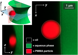
Figure 2: (Color online) Horizontal and vertical slices of a confocal micrograph of a single PMMA sphere electrostatically bound to the neck of a capillary bridge droplet. Top Left: Schematic of the geometry of the particle and interface. The curvature of the capillary bridge is exaggerated for clarity. Main Figure: The dashed white curves show the result of an edge-finding routine designed to measure the contact angle. For this particle, $\theta_{C}=$180\text{\,}\mathrm{\SIUnitSymbolDegree}$^{+$0\text{\,}\mathrm{\SIUnitSymbolDegree}$}_{-$9\text{\,}\mathrm{\SIUnitSymbolDegree}$}$.

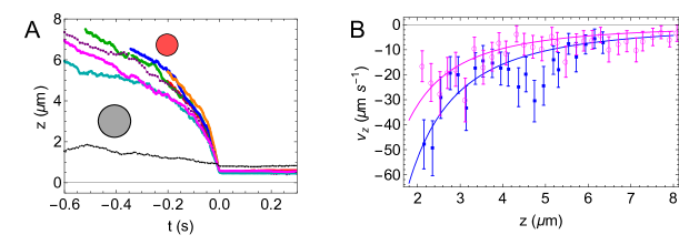
Figure 3: (Color online) (A) The colored trajectories are obtained by digital holographic microscopy of seven different $d=$1.1\text{\,}\mathrm{\SIUnitSymbolMicro m}$$ colloidal particles approaching the oil/aqueous phase interface. For each trajectory, we have set $t=0$ as the time of the attachment event, and $z=0$ as the position of the fluid interface. The charged particles are strongly attracted to the interface, achieving speeds of up to $80\text{\,}\mathrm{\SIUnitSymbolMicro m}\text{\,}{\mathrm{s}}^{-1}$. For comparison, these particles have a sedimentation velocity of $0.04\text{\,}\mathrm{\SIUnitSymbolMicro m}\text{\,}{\mathrm{s}}^{-1}$. We have also plotted (in black) the trajectory of a $d=$1.6\text{\,}\mathrm{\SIUnitSymbolMicro m}$$ PMMA particle in a system where the oil phase consists of pure decane Wang et al. (2013). In the absence of CHB, the particle is far less charged, and approaches the interface much more slowly than in the presence of CHB. The red and gray disks indicate the sizes of the colloidal particles, to scale on the $z$-axis. (B) Plot of the velocities of two of the trajectories, as a function of distance from the interface. The error bars indiate the expected width of the velocity distribution, calculated from the bulk diffusion constant $D_{0}$. For each data set, the best fits of the model given by Eqs. (1), (2) and (3) are also shown.

II.0.3 Colloidal Particles

The PMMA microparticles are sterically stabilized with covalently bound poly(12-hydroxystearic acid) Elsesser and Hollingsworth (2010). Such particles have a surface charge that might be caused by adsorption of positively charged species resulting from the decomposition of CHB Leunissen (2007), chemical coupling of an amine catalyst during particle synthesis van der Linden et al. (2015), or some combination of these mechanisms. In some of our experiments, we use spheres that are fluorescently labeled with absorbed rhodamine 6G dye Elsesser et al. (2011). We find that dyeing the particles does not affect their measured interactions.

III Measurement of the Contact Angle $\theta_{C}$

To verify that our particles remain entirely immersed in the oil and are not wetted by the aqueous phase, we measure their contact angle directly by fluorescent confocal microscopy. We do this by preparing a low-concentration dispersion of PMMA particles of mean diameter $2.6\text{\,}\mathrm{\SIUnitSymbolMicro m}$ in oil, and flow the dispersion into a channel containing several capillary bridges of the aqueous phase. To create these capillary bridges, we first use a sprayer to deposit droplets (of typical diameter $10\text{\,}\mathrm{\SIUnitSymbolMicro m}100\text{\,}\mathrm{\SIUnitSymbolMicro m}$) of the aqueous phase on a cover slip. We then place the cover slip, droplet side down, on Dura-lar spacers of thickness $25\text{\,}\mathrm{\SIUnitSymbolMicro m}$ which have been placed on a microscope slide. The larger droplets come into contact with the microscope slide, and spontaneously form capillary bridges. We use a two-channel Leica TCS SP5 II confocal microscope, with a $63\times$ NA 1.4 oil-immersion objective lens to simultaneously image the particles and the aqueous phase. For these studies, the aqueous phase is fluorescently labeled by replacing some or all of the NaCl with fluorescein sodium salt. Since the oil and aqueous phases are refractive-index matched to within approximately 1%, optical artifacts arising from the curvature of the interface are minimized.

As shown in Fig. 2, some of the particles bind to the neck of a capillary bridge, presumably by electrostatic forces. Using inbuilt edge-detection algorithms from the commercial software package Mathematica, we identify the edges of the capillary bridge and the colloidal particle. The contact angle is calculated from these data. A typical confocal slice, overlaid with the results of the edge-finding routine, is shown in Fig. 2. For our system, we measure the best-fit contact angle of the particles to be in the range $171\text{\,}\mathrm{\SIUnitSymbolDegree}180\text{\,}\mathrm{\SIUnitSymbolDegree}$, consistent with the results of Ref. Leunissen et al. (2007). All measurements are consistent with a contact angle of $180\text{\,}\mathrm{\SIUnitSymbolDegree}$.

IV Colloid-Interface Interaction

We probe the interaction of individual colloidal spheres with a flat, horizontal oil/aqueous phase interface by measuring their trajectories as they move through the oil phase toward the interface. Because the particles move at speeds up to $80\text{\,}\mathrm{\SIUnitSymbolMicro m}\text{\,}{\mathrm{s}}^{-1}$, too fast to track with confocal microscopy, we measure their trajectories with digital holographic microscopy. In this technique, an incident monochromatic plane wave scatters from a spherical colloidal particle. Using the apparatus described in Refs. Wang et al. (2013) and Kaz et al. (2011), we digitally record the image that results from interference of the scattered light with the incident plane wave Gabor (1949); Schnars and Jüptner (2002). Fitting the interference pattern predicted by Lorentz-Mie theory to the recorded hologram Lee et al. (2007) gives the particle’s three-dimensional position with $3\text{\,}\mathrm{nm}$ precision over a $50\text{\times}50\text{\times}50\text{\,}\mathrm{\SIUnitSymbolMicro m}$ volume at time intervals as low as $1\text{\,}\mathrm{ms}$. Since the oil and aqueous phases have well-matched refractive indices, we fit the data using functions appropriate for scattering from a dielectric sphere immersed in a medium of uniform refractive index Hol . To avoid interference from multiple particles in the same image, PMMA-in-oil dispersions are prepared at volume fractions below ${10}^{-6}$. As well as position data, the holographic measurements yield estimates for the diameters of the particles, with nanometer precision, and their refractive indices, which can be used for consistency checks. The colloidal particles we use for these and all subsequent studies have a mean diameter $d=$1.08\text{\,}\mathrm{\SIUnitSymbolMicro m}$$ and polydispersity 5%.

To understand the observed trajectories of the particles as they approach the interface (Fig. 3), we construct an equation of motion involving the electrostatic force and drag. Because the aqueous phase contains dissolved salt ions that act as free charges, we treat it as a good conductor. A sphere of charge $q$ whose center is at height $z$ above a flat conducting surface is attracted towards its image charge with a force Jackson (1998)

$$F_{z}(z)=-\frac{q^{2}}{16\pi\epsilon_{r}\epsilon_{0}z^{2}}.$$ (1)

Because the motion is overdamped, the speed with which the sphere approaches the interface is given by

$$v_{z}(z)=\frac{F_{z}(z)}{\gamma_{\perp}(z)},$$ (2)

where $\gamma_{\perp}(z)$ is the viscous drag coefficient for motions perpendicular to the fluid-fluid interface located in the plane $z=0$. Lee and Leal Lee et al. (1979) find that

$$\frac{\gamma_{\perp}(z)}{\gamma_{0}}=1+\frac{3}{16}\frac{d}{z}\frac{2+3\lambda}{1+\lambda}+\left(\frac{3}{16}\frac{d}{z}\frac{2+3\lambda}{1+\lambda}\right)^{2}+O\!\left\{\frac{d^{3}}{z^{3}}\right\},$$ (3)

where $\lambda=\mu_{\text{aq}}/\mu_{\text{oil}}$ is the ratio of dynamic viscosities of the two fluid phases and $\gamma_{0}=3\pi\mu_{\text{oil}}d$ is the Stokes drag on a sphere far from any boundaries. For our system, $\mu_{\text{aq}}=$23\text{\,}\mathrm{mPa}\text{\,}\mathrm{s}$$ (from tabulated values) and $\mu_{\text{oil}}=$1.7\text{\,}\mathrm{mPa}\text{\,}\mathrm{s}$$ (from our measurements of the particle diameter and diffusion constant in bulk oil) so that $\lambda=$14$$. We estimate $D_{0}$, the 3D diffusion constant of the particles far from any boundaries, by measuring $D_{\parallel}(z)$, the diffusion coefficient parallel to the interface. We calculate $D_{\parallel}(z)$ from those parts of the trajectories where $z>$2\text{\,}\mathrm{\SIUnitSymbolMicro m}$$. From the hydrodynamic theory in Ref. Lee et al. (1979), we estimate that the error in approximating $D_{0}$ by $D_{\parallel}(z>$2\text{\,}\mathrm{\SIUnitSymbolMicro m}$)$ is around $6\text{\,}\mathrm{\char 37\relax}$. We then use the fluctuation-dissipation relation, $\gamma_{0}=k_{B}T/D_{0}$, to obtain the drag coefficient at the absolute temperature $T=$293\text{\,}\mathrm{K}$$. A typical value for the spheres in this study is $\gamma_{0}=$ $17\text{\,}\mathrm{nN}\text{\,}\mathrm{s}\text{\,}{\mathrm{m}}^{-1}$.

Applying the model consisting of Eqs. (1), (2) and (3) to the data in Fig. 3 yields good agreement with the measured velocities for a mean sphere charge $q=$530\pm 30.\text{\,}\mathrm{e}$$, where e is the elementary charge, and the uncertainty is given by the standard error of the mean.

A priori, we cannot exclude the possibility of the presence of significant amounts of (positive or negative) surface charge $\sigma$ on the oil/aqueous phase interface Leunissen et al. (2007), which would require including an extra force $q\sigma/\epsilon_{r}\epsilon_{0}$ on the right-hand side of Eq. (1). Treating $\sigma$ as a fit parameter in this expanded model yields as an upper bound $\left|\sigma\right|<$0.2\text{\,}\mathrm{e}\mathrm{/}\mathrm{{}^{2}}\mathrm{\SIUnitSymbolMicro}\mathrm{m}$$, but neither improves the quality of the fits nor significantly affects our estimate of the particle charge $q$. We therefore omit $\sigma$ from the model. We also neglect the gravitational force because, over the measured range of $z$, it is negligible compared to the image-charge interaction: $\left|F_{\text{grav}}\right|<0.02\left|F_{z}\right|$.

These measurements establish that the force drawing the PMMA spheres to the interface is consistent with image-charge attraction and provide an estimate of the single-sphere charge. We next investigate how that charge influences the interaction between spheres at the interface.

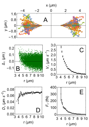
Figure 4: (Color online) Stages in the analysis of the data from the catch-and-release experiment to probe the repulsive force between a specific pair of interfacial colloids. (A) Overlay of 180 post-release trajectories of a single pair of colloidal particles. At each instant, the positions are plotted in the center-of-mass frame. (B) Frame-to-frame radial displacement, plotted as a function of center-to-center separation $r$. (C) Radial velocity, obtained by binning and averaging the data in B. (D) The radial diffusion constant $D_{r}(r)$ is obtained from the variance of data in each bin. The dashed line is a guide to the eye, and highlights the $r$-dependence of $D_{r}$, which we attribute to hydrodynamic interaction between the particles. We obtain the radial drag coefficient $\gamma_{r}(r)$ by using the fluctuation-dissipation relation, $\gamma_{r}(r)=k_{B}T/D_{r}(r)$. (E) The radial force is found by multiplying the velocity by the drag coefficient, $F_{r}(r)=\gamma_{r}(r)V_{r}(r)$.

V Pair Interaction of Interfacial Colloids

In this section, we describe the results of three independent experiments for measuring the force between interfacially bound colloidal particles as a function of interparticle separation $r$. The results are all consistent with an electrostatic model in which the charge $q$ on a single sphere is $570\pm 30.\text{\,}\mathrm{e}$, which is in turn consistent with the result described in the previous section.

We treat the colloidal particles as spheres of uniform surface charge sitting directly above the aqueous phase, which, as in the previous section, plays the role of a conducting substrate. As shown in Fig. 1(A), pairs of spheres are repelled by each other’s charges, but are attracted to their neighbors’ image charges. All our measurements take place in the regime where interparticle separations are large compared to the colloid diameter, but small compared to the Debye length in the oil phase, so that $d^{2}\ll r^{2}\ll\lambda_{D}^{2}$. In this limit, the net interaction force, $F_{r}(r)$, between pairs of spheres with center-to-center separation $r$ takes a dipolar form,

$$F_{r}(r)=-\frac{q^{2}}{4\pi\epsilon_{r}\epsilon_{0}}\frac{\text{d}}{{\text{dr}}}\Bigg{(}\frac{1}{r}-\frac{1}{(r^{2}+d^{2})^{1/2}}\Bigg{)}\simeq\frac{3B}{r^{4}},$$ (4)

where the force constant $3B$ is related to the particle charge by $B=q^{2}d^{2}/8\pi\epsilon_{r}\epsilon_{0}$.

V.1 “Catch-and-Release” Laser Tweezer Experiments

Our first measurement of the repulsive force between a pair of interfacial particles proceeds by forcing the particles close together with a pair of optical tweezers and then releasing them. We record and analyze the resulting trajectories to find the interparticle force, as illustrated in Fig. 4.

For these experiments, and also those of Section V.3, we prepare samples that contain many small (diameter $100\text{\,}\mathrm{\SIUnitSymbolMicro m}500\text{\,}\mathrm{\SIUnitSymbolMicro m}$), almost-flat interfaces that are isolated from each other. To make these interfaces, a cover slip is immeresed in a bath of KOH-saturated isopropanol for $1\text{\,}\mathrm{h}$ prior to undergoing the treatment described in Section II.0.1. We use a sprayer to deposit droplets of the aqueous phase onto the cover slip, which is then incorporated into the construction of a capillary channel. Finally, the channel is filled with the particle dispersion and sealed with Norland optical adhesive. Following this protocol, each droplet of the aqueous phase forms a roughly spherical cap on the glass surface, with a contact angle of $1\text{\,}\mathrm{\SIUnitSymbolDegree}$ or less. The resulting interface is flat enough to allow bright-field imaging of interfacial particles, which adsorb to the interface because of the electrostatic attraction described in Section IV. Effectively random factors, such as how far a given droplet is from the entrance of the capillary channel, influence how many particles are deposited on each interface. Thus, within a in a single sample cell, we obtain many isolated interfaces, each with a different interfacial density.

To measure the interparticle force, we first identify an interface at sufficently low particle density that only two spheres are in the field of view of the microscope. A particle tracking algorithm then locates the spheres Crocker and Grier (1994, 1996). Once located, the spheres are confined in holographic optical traps projected at their position (“catch”) Curtis et al. (2002); Dufresne and Grier (1998); Polin et al. (2005). The holographic trapping system is created with a $1064\text{\,}\mathrm{nm}$ laser (IPG Photonics YLR-10-1064-LP) whose wavefronts are modified using a computer-controlled liquid-crystal spatial light modulator (Holoeye Pluto). The resulting light pattern is relayed to an objective lens (Nikon Plan Apo, NA 1.45 $100\times$, oil immersion) that focuses the traps into the sample. The traps drag the particles towards one another until they reach a pre-assigned minimum distance, at which point the traps are instantaneously displaced tens of microns in the direction perpendicular to the imaging plane, allowing the particles to move freely along the interface (“release”). The trajectories of the particles are recorded by video microscopy, and the coordinates of the centers of the particles, $\mathbf{r}_{1}$ and $\mathbf{r}_{2}$, are measured using publicly available tracking routines Crocker and Grier (1996); Cro . This procedure, shown in Fig. 1(B), is fully automated, and, for a given pair of particles, is repeated as many as several hundred times.

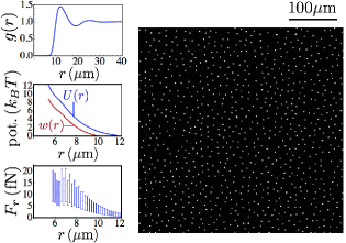
Figure 5: (Color online) Main Image: Confocal micrograph of PMMA particles bound to a glycerol/water interface. This image is a single snapshot taken from a $1\text{\,}\mathrm{h}$ movie, with an average particle density of 0.005$\,\mu$m^-2. Left Column: A series of plots showing: (i) $g(r)$, from all frames of the movie; (ii) the potential of mean force $w(r)=-k_{B}T\log{g}$ and the pair potential $U(r)$. We use the Ornstein-Zernike equation to obtain $U(r)$ from $g(r)$; (iii) the radial force, obtained from $U(r)$ by numerical differentiation.

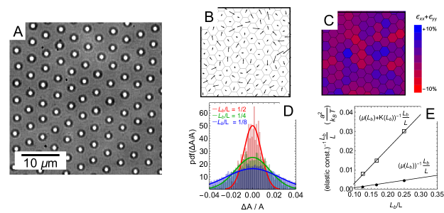
Figure 6: (Color online) Finding the elastic moduli of a 2D colloidal crystal from video microscopy. (A) Snapshot taken from a movie of $100$ statistically independent frames. The lattice constant $a$ is $4.3\text{\,}\mathrm{\SIUnitSymbolMicro m}$. We analyze the fluctuations within a square box of side length $L=8a=$34\text{\,}\mathrm{\SIUnitSymbolMicro m}$$. (B) The instantaneous displacement field $\mathbf{u}$ corresponding to the particle configuration shown in panel A. For clarity, the magnitude of the displacements is exaggerated by a factor of 5. Also shown is the Voronoi tesselation, computed from the average particle positions. (C) Trace of the strain tensor, $\epsilon_{xx}(\mathbf{r},t)+\epsilon_{yy}(\mathbf{r},t)$, calculated from the displacement field shown in panel B. (D) Probability distribution function of the dilatation strain $(\Delta A/A)$ for three different sub-region sizes $L_{b}/L$. Solid curves are Gaussian fits to the data. (E) We obtain elastic moduli of $K=40~{}k_{B}T${\mathrm{\SIUnitSymbolMicro m}}^{-2}$$ and $\mu=6~{}k_{B}T${\mathrm{\SIUnitSymbolMicro m}}^{-2}$$, which, via Eqs. (6), give $\Gamma=$305\pm 35.$$. Thus, for an interparticle separation of $4.3\text{\,}\mathrm{\SIUnitSymbolMicro m}$, the interparticle force is $F_{r}=$110\pm 30.\text{\,}\mathrm{fN}$$.

Once a particle is released from the optical traps, its motion results from a combination of interaction with the other particle, and diffusion. For two subsequent frames, the displacement of the particles along the radial direction in the center-of-mass reference frame is

$$\Delta_{r}(t)=\left[\mathbf{r}(t+\tau)-\mathbf{r}(t)\right]\cdot\mathbf{\hat{r}}(t),$$ (5)

where $\mathbf{r}(t)$ is the instantaneous separation at time $t$, $\mathbf{r}(t)=\mathbf{r}_{2}(t)-\mathbf{r}_{1}(t)$, and $\tau=$16.7\text{\,}\mathrm{ms}$$ is the time interval between video fields. The relative velocity, $v_{r}(r)=\Delta_{r}/\tau$, as well as the separation-dependent drag coefficient in the radial direction $\gamma_{r}(r)$, is found by combining the data from multiple releases, and plotting $\Delta_{r}$ as a function of interparticle separation $r$. The data are divided into bins along the $r$-axis, as shown in Fig. 4, and the interparticle force is obtained by using the overdamped equation of motion, $F_{r}(r)=\gamma_{r}(r)v_{r}(r)$ Crocker and Grier (1994); Crocker (1997); Sainis et al. (2007). The results of 10 such experiments, on different pairs of particles, are shown in Fig. 7(A). Fitting Eq. (4) to this data gives $q=$580\pm 30.\text{\,}\mathrm{e}$$, which is consistent with the value obtained from the colloid-interface experiments in Section IV.

V.2 Pair Correlation Function Experiments

In a second experiment to measure the pair interaction, we measure the pair correlation function $g(r)$ of a system of interfacial particles at low areal density $\rho$. We use the Ornstein-Zernike equation from liquid state theory, with the hypernetted chain approximation, to obtain the pair potential $U(r)$ from $g(r)$ Behrens and Grier (2001); Hansen and McDonald (2006), and finally calculate $F_{r}(r)$ by numerical differentiation. To sample $g(r)$ at the low densities this method requires, we first half-fill a capillary tube with the aqueous phase. We then place the filled end of the capillary tube into a sample vial containing the particle dispersion. As the oil flows into the tube, thin patches of the aqueous phase are left behind on the top and bottom glass surfaces. These patches, held in place by pinning of the contact line, are typically $0\text{\,}\mathrm{\SIUnitSymbolMicro m}2\text{\,}\mathrm{\SIUnitSymbolMicro m}$ thick, and millimeters in diameter. We are thus able to image regions of uniform density as large as $0.3\text{\,}{\mathrm{mm}}^{2}$, and which contain hundreds of particles. We use a Leica TCS SP5 II confocal microscope, mounted with a $10\times$ air objective lens, to collect movies which are typically $1\text{\,}\mathrm{h}2\text{\,}\mathrm{h}$ in length. Using publicly available software Cro , we find the positions of the particles in each frame and obtain $g(r)$ for each movie. Fig. 5 shows a snapshot of a typical sample, together with the stages of the anaysis.

To estimate the error in finding the force in this manner, we perform a series of Monte-Carlo simulations of point particles interacting via a set of known interaction potentials. We choose the interaction potentials and densities in the simulations so that they produce pair correlation functions similar to those observed in the experiments. From each simulation, we calculate $g(r)$, and then apply the Ornstein-Zernike method described above to obtain $U(r)$ and $F_{r}(r)$. We compare the $F_{r}(r)$ obtained from $g(r)$ to the $F_{r}(r)$ curve calculated directly from the potential that we use in the simulation. The error $\Delta F_{r}$ is given by the difference between these two values. Since the fractional error $\Delta F_{r}/F_{r}$ does not depend strongly on $r$, $\rho$, or the parameters describing the interaction potential, we take it to be constant, $\Delta F_{r}/F_{r}=0.5$. This value is assumed when plotting error bars such as those shown in Fig. 5.

Fig. 7(B) shows the results of applying the Ornstein-Zernike inversion procedure to samples of interfacial colloids at two different areal densities. For each sample, we repeat the measurement one, two and four days after preparation to confirm that the results for $g(r)$ are time-independent, and thus reflect equilibrium properties. Fitting this data to Eq. (4) gives $q=$540\pm 30.\text{\,}\mathrm{e}$$, which is consistent both with the value obtained from the colloid-interface interaction experiments in Section IV and with other pair interaction experiments described in this section.

V.3 Crystal Elasticity Experiments

Our third approach for measuring the pair interaction takes advantage of the fact that, when confined to an interface at sufficiently high areal density, colloidal monolayers form a hexagonally-ordered solid phase, which is stable over time-scales of many weeks . This colloidal solid is soft enough that thermal fluctuations of the particle positions can be measured using video or confocal microscopy. From the resulting trajectories, we can estimate the crystal’s bulk modulus, $K$, and shear modulus, $\mu$. These elastic constants are related to the crystal’s interaction parameter, $\Gamma$, which yields the pair potential at the mean interparticle separation $a$ Weiss et al. (1998); Zahn et al. (2003). Unlike the previously discussed measurements, which yield functional forms for the separation-dependent interaction, interaction measurements based on lattice elasticity require us to assume a functional form. However, since this measurement takes place at high areal density, it can confirm the pair-wise additivity of the interactions.

To determine the interparticle force and the elastic constants, we first measure the instantaneous strain and rotation. For a displacement field $\mathbf{u}(\mathbf{r},t)$ at position $\mathbf{r}$ and time $t$, the instantaneous strain and rotation tensors are defined as

$$\epsilon_{ij}(\mathbf{r},t) =\frac{1}{2}\left[\partial_{i}u_{j}(\mathbf{r},t)+\partial_{j}u_{i}(\mathbf{r},t)\right]\quad\text{and}$$

$$\theta_{ij}(\mathbf{r},t) =\frac{1}{2}\left[\partial_{i}u_{j}(\mathbf{r},t)-\partial_{j}u_{i}(\mathbf{r},t)\right],$$

respectively, where $i,j\in\{x,y\}$. Adapting these definitions to include a displacement field $\mathbf{u}$ defined at a discrete set of lattice points and times, we use the lattice calculus methods described in the Appendix to calculate the strain and rotation tensors from the measured set of particle positions.

For a region of area $A$, the dilatation strain is given by

$$\frac{\Delta A(t)}{A}=\frac{1}{A}\int_{A}\left[\epsilon_{xx}(\mathbf{r},t)+\epsilon_{yy}(\mathbf{r},t)\right]\,d^{2}\mathbf{r},$$

and the local rotation is

$$\Delta\theta(t)=\frac{1}{A}\int_{A}\theta_{xy}(\mathbf{r},t)\,d^{2}\mathbf{r}.$$

If we assume equipartition of energy, the variances in these quantities in a box of side length $L_{b}$ are related to the finite-size bulk and shear moduli $K(L_{b})$ and $\mu(L_{b})$ by Zahn et al. (2003)

$$\mathrm{Var}\!\left\{\frac{\Delta A(t)}{A}\right\}_{L_{b}} =\frac{k_{B}T}{A\left[K(L_{b})+\mu(L_{b})\right]}\quad\text{and}$$

$$\mathrm{Var}\!\left\{\Delta\theta(t)\right\}_{L_{b}} =\frac{k_{B}T}{2A\,\mu(L_{b})}.$$

The thermodynamic limits of the elastic constants are obtained by the finite-sized scaling procedure Sengupta et al. (2000) shown in Fig. 6(E).

The elastic moduli are related to the potential energy $U(r)=Br^{-3}$ of the particles’ pair repulsion at the nearest-neighbor separation, $r=a$. In terms of the dimensionless interaction parameter $\Gamma=B(\pi\rho)^{3/2}/k_{B}T$, we expect, in the high-density limit Keim et al. (2004),

$$\Gamma=\frac{a^{2}}{0.3461\,k_{B}T}\,\mu\quad\text{and}\quad\Gamma=\frac{a^{2}}{3.461\,k_{B}T}\,K.$$ (6)

Thus, each elastic constant provides a measurement of $\Gamma$. We take the average of these measurements to be our estimate for $\Gamma$, and half their difference to be the corresponding uncertainty $\Delta\Gamma$. Finally, we estimate the nearest-neighbor interaction force $F_{r}(a)=3Ba^{-4}=3k_{B}T\Gamma(\pi\rho)^{-3/2}a^{-4}$.

We confirm the accuracy of our implementation of this protocol through molecular dynamics simulations perfomed using the HOOMD-blue suite Anderson et al. (2008); Glaser et al. (2015); hoo . For parameter values similar to those of the experiment, our analysis of the particle trajectories accurately reproduces the interaction parameter $\Gamma$ and the interparticle force $F_{r}$.

Fig. 7(C) shows the results of applying this analysis to five different samples. We restrict our data collection to crystals that have lattice constants between $a=$3\text{\,}\mathrm{\SIUnitSymbolMicro m}$$ and $5\text{\,}\mathrm{\SIUnitSymbolMicro m}$. Crystals with $a\lesssim$3\text{\,}\mathrm{\SIUnitSymbolMicro m}$$ do not satisfy the far-field assumption $r^{2}\gg d^{2}$, while those with $a\gtrsim$5\text{\,}\mathrm{\SIUnitSymbolMicro m}$$ do not have high enough density to justify the use of Eq. (6). Fitting Eq. (4) to the plotted data, we find that the charge $q=$590\pm 20.\text{\,}\mathrm{e}$$. As Table 1 shows, this value is consistent with the other pair interaction experiments, and, within two standard deviations, is also consistent with the results of the colloid-interface experiments.

In our experiments, we have observed the behavior of specific pairs of particles far away from any others (tweezer experiments), as well as systems of many particles in both the low density ($g(r)$ experiment) and the high density (crystal elasticity experiment) limits. The fact that the measured charge is consistent in all these cases implies that the interaction is pairwise additive over the range of interparticle separations explored by our experiments. This contrasts with other systems of colloidal particles dispersed in oil Merrill et al. (2009), and may have implications for understanding the origin of the surface charge on the particles.

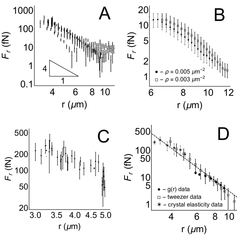
Figure 7: Log-log plots of the results of three experiments to find forces between interfacial colloids. (A) Results of the catch-and-release laser tweezer experiment, for 10 pairs of interfacial particles. (B) Results of finding the interparticle force via the pair potential $g(r)$, for two samples at different areal densities. (C) Results of experiments where we found the interparticle force via the elastic moduli of 2D colloidal crystals. Each data point corresponds to a different video of a fluctuating lattice. (D) The data from panels A, B and C are divided into bins. For each data set, the mean in each bin is plotted. Error bars indicate the spread of the data in a given bin: standard deviation for data sets A and C, maximum deviation from the mean in the case of B. The dashed line is a fit of all the data to Eq. (4), which gives $q=$570\pm 30.\text{\,}\mathrm{e}$$.

VI Conclusions

In this work, we study the behavior of a system of charged colloids in the vicinity of a fluid interface. We show that, in the absence of wetting by the aqueous phase, this behavior is governed by electrostatics alone: individual colloids interact with the interface via image-charge attraction, while particles that are already interfacially bound interact with their neighbors as charge-image charge dipoles. Our model, in which the particle charge $q$ is the only fit parameter, is consistent with data from the four independent experiments we have performed.

In our system, interactions between interfacial particles are pairwise-additive, are constant over time-scales of weeks, and are homogenous enough to allow the formation of defect-free crystals over length-scales of tens of lattice spacings. The system is thus well-suited to the study of problems in fundamental condensed matter physics, for example the phase behavior of repulsive particles in 2D Deutschländer et al. (2015); Qi et al. (2014), or the structure and dynamics of topological defects in curved spaces Irvine et al. (2010, 2012); Kusumaatmaja and Wales (2013). Moreover, we can now hope to use our knowledge of electrostatic interactions in systems of interfacial colloids to better understand the behavior of more complex systems, such as those with partial wetting.

	$q$ (e)
colloid-interface experiment	$\quad 530\pm 30\quad$
laser tweezer experiment	$\quad 580\pm 30\quad$
$g(r)$ experiment	$\quad 540\pm 30\quad$
crystal elasticity experiment	$\quad 590\pm 20\quad$

Table 1: Particle charge found in each of the four experiments described in this paper.

This work was supported primarily by the National Science Foundation under Award No. DMR-1105417. Partial support was provided by NASA, through Award No. NNX13AR67G, and the MRSEC program of the National Science Foundation through Award Nos. DMR-1420073 and DMR-1420570. G. I. G-G. acknowledges CONACYT for financial support via the program Catedras CONACYT para Jovenes Investigadores. The authors would like to acknowledge fruitful discussion with Dan Evans, Gary L. Hunter, Eric DeGiuli and Aleksandar Donev at New York University.

*

Appendix A Finding Strain and Rotation Tensors from Particle Trajectories

Here we outline how we use a discretized version of the divergence theorem from vector calculus to the calculate the strain and rotation tensor from the particle trajectories obtained from video microscopy.

We first define the particle’s equilibrium position. After subtracting uniform drift, we still need to eliminate effects which are due to slow expansion, compression or rotation of the lattice, as well as the long-wavelength fluctations which are characteristic of 2D solids Gasser et al. (2010). To do this, we use a moving average of the particle’s position using time window which is typically 20 times the relaxation time of an individual particle, as computed from the mean square displacement. At each frame of the movie, the displacement $\mathbf{u}(\alpha)$ of particle $\alpha$ is calculated relative to this moving average.

Once we obtain the displacement field $\mathbf{u}$ for a given frame of the movie, we need to calculate the strain and rotation tensors, which requires taking derivatives of $\mathbf{u}$. In order to do this, we use the Voronoi construction to partition the field of view into cells associated with each lattice site. This construction provides a well-defined set of nearest neighbors for each particle, which does not change over the course of the movies. For an arbitrary vector field $\mathbf{v}$, the matrix of partial derivatives $\partial_{i}v_{j}(\alpha)$ of particle $\alpha$ can be calculated by using a discrete version of the divergence theorem DeGiuli and McElwaine (2011). This works as follows: for every particle $\beta$ that neighbors $\alpha$, the particles share an edge of a Voronoi cell, which we label ($\alpha,\beta$). For each edge, we define the vector $\mathbf{v}(\alpha,\beta)$ as the average of $\mathbf{v}(\alpha)$ and $\mathbf{v}(\beta)$, while the normal vector $\mathbf{\hat{n}}(\alpha,\beta)$ and the edge length $\ell(\alpha,\beta)$ are given by the geometry of the Voronoi cell. Using this notation, the divergence of $\mathbf{v}$ at particle $\alpha$ is given by

$$\nabla\cdot\mathbf{v}(\alpha)=\frac{1}{A(\alpha)}\sum_{\beta\text{ n.n.}\alpha}\ell(\alpha,\beta)\left(\mathbf{v}(\alpha,\beta)\cdot\mathbf{\hat{n}}(\alpha,\beta)\right),$$

where $A(\alpha)$ is the area of the Voronoi cell of particle $\alpha$, and the sum is taken over all particles $\beta$ which are nearest neighbors to particle $\alpha$. For appropriate choice of $\mathbf{v}$, the components of the strain and rotation tensors can be found at each lattice site. For instance, $\epsilon_{xx}=\partial_{x}u_{x}=\nabla\cdot\mathbf{v}$, where $\mathbf{v}=(u_{x},0)$.

References

- Ramsden (1903) W. Ramsden, Proceedings of the Royal Society of London 72, 156 (1903).
- Frydel et al. (2007) D. Frydel, S. Dietrich, and M. Oettel, Physical Review Letters 99, 118302 (2007).
- Oettel and Dietrich (2008) M. Oettel and S. Dietrich, Langmuir 24, 1425 (2008).
- Cui et al. (2013) M. Cui, T. Emrick, and T. P. Russell, Science 342, 460 (2013).
- Poulichet and Garbin (2015) V. Poulichet and V. Garbin, Proceedings of the National Academy of Sciences 112, 5932 (2015).
- Pieranski (1980) P. Pieranski, Physical Review Letters 45, 569 (1980).
- Aveyard et al. (2002) R. Aveyard, B. Binks, J. Clint, P. Fletcher, T. Horozov, B. Neumann, V. Paunov, J. Annesley, S. Botchway, D. Nees, A. Parker, A. Ward, and A. Burgess, Physical Review Letters 88, 246102 (2002).
- Park et al. (2014) B. J. Park, B. Lee, and T. Yu, Soft Matter 10, 9675 (2014).
- Parolini et al. (2015) L. Parolini, A. D. Law, A. Maestro, Buzza, and P. Cicuta, Journal of Physics: Condensed Matter 27, 194119 (2015).
- McGorty et al. (2010) R. McGorty, J. Fung, D. Kaz, and V. N. Manoharan, Materials Today 13, 34 (2010).
- Reynaert et al. (2006) S. Reynaert, P. Moldenaers, and J. Vermant, Langmuir 22, 4936 (2006).
- Ghezzi and Earnshaw (1997) F. Ghezzi and J. C. Earnshaw, Journal of Physics: Condensed Matter 9, L517 (1997).
- Park and Furst (2011) B. J. Park and E. M. Furst, Soft Matter 7, 7676 (2011).
- Gao et al. (2014) P. Gao, X. Xing, Y. Li, T. Ngai, and F. Jin, Scientific Reports 4 (2014).
- Park et al. (2010) B. J. Park, J. Vermant, and E. M. Furst, Soft Matter 6, 5327 (2010).
- Chen et al. (2009) W. Chen, S. Tan, Y. Zhou, T.-K. Ng, W. T. Ford, and P. Tong, Physical Review E 79 (2009).
- Aveyard et al. (1999) R. Aveyard, J. H. Clint, D. Nees, and V. N. Paunov, Langmuir 16, 1969 (1999).
- Masschaele et al. (2010) K. Masschaele, B. J. Park, E. M. Furst, J. Fransaer, and J. Vermant, Physical Review Letters 105, 048303 (2010).
- Stamou et al. (2000) D. Stamou, C. Duschl, and D. Johannsmann, Physical Review E 62, 5263 (2000).
- Kaz et al. (2011) D. M. Kaz, R. McGorty, M. Mani, M. P. Brenner, and V. N. Manoharan, Nature Materials 11, 138 (2011).
- Leunissen et al. (2007) M. E. Leunissen, A. van Blaaderen, A. D. Hollingsworth, M. T. Sullivan, and P. M. Chaikin, Proceedings of the National Academy of Sciences 104, 2585 (2007).
- Irvine et al. (2010) W. T. M. Irvine, V. Vitelli, and P. M. Chaikin, Nature 468, 947 (2010).
- Leunissen (2007) M. E. Leunissen, Manipulating Colloids with Charges & Electric Fields, Ph.D. thesis, Utrecht University (2007).
- Looyenga (1965) H. Looyenga, Physica 31, 401 (1965).
- Zwanikken et al. (2008) J. Zwanikken, J. de Graaf, M. Bier, and R. van Roij, Journal of Physics: Condensed Matter 20, 494238 (2008).
- Wang et al. (2013) A. Wang, D. M. Kaz, R. R. McGorty, and V. N. Manoharan, in 4th International Symposium on Slow Dynamics in Complex Systems: Keep Going Tohoku, Vol. 1518 (American Institute of Physics, 2013) pp. 336–343.
- Elsesser and Hollingsworth (2010) M. T. Elsesser and A. D. Hollingsworth, Langmuir 26, 17989 (2010).
- van der Linden et al. (2015) M. N. van der Linden, J. C. P. Stiefelhagen, G. Heessels-Gürboğa, J. E. S. van der Hoeven, N. A. Elbers, M. Dijkstra, and A. van Blaaderen, Langmuir 31, 65 (2015).
- Elsesser et al. (2011) M. T. Elsesser, A. D. Hollingsworth, K. V. Edmond, and D. J. Pine, Langmuir 27, 917 (2011).
- Gabor (1949) D. Gabor, Proceedings of the Royal Society of London A: Mathematical, Physical and Engineering Sciences 197, 454 (1949).
- Schnars and Jüptner (2002) U. Schnars and W. P. Jüptner, Measurement Science and Technology 13, R85 (2002).
- Lee et al. (2007) S.-H. Lee, Y. Roichman, G.-R. Yi, S.-H. Kim, S.-M. Yang, A. van Blaaderen, P. van Oostrum, and D. G. Grier, Optics Express 15, 18275 (2007).
- (33) https://github.com/manoharan-lab/holopy.
- Jackson (1998) J. D. Jackson, Classical Electrodynamics Third Edition, 3rd ed. (Wiley, 1998).
- Lee et al. (1979) S. H. Lee, R. S. Chadwick, and L. G. Leal, Journal of Fluid Mechanics 93, 705 (1979).
- Crocker and Grier (1994) J. C. Crocker and D. G. Grier, Physical Review Letters 73, 352 (1994).
- Crocker and Grier (1996) J. C. Crocker and D. G. Grier, Journal of Colloid and Interface Science 179, 298 (1996).
- Curtis et al. (2002) J. E. Curtis, B. A. Koss, and D. G. Grier, Optics Communications 207, 169 (2002).
- Dufresne and Grier (1998) E. R. Dufresne and D. G. Grier, Review of Scientific Instruments 69, 1974 (1998).
- Polin et al. (2005) M. Polin, K. Ladavac, S.-H. Lee, Y. Roichman, and D. G. Grier, Optics Express 13, 5831 (2005).
- (41) http://www.physics.emory.edu/faculty/weeks//idl/.
- Crocker (1997) J. C. Crocker, J. Chem. Phys. 106, 2837 (1997).
- Sainis et al. (2007) S. K. Sainis, V. Germain, and E. R. Dufresne, Physical Review Letters 99 (2007).
- Behrens and Grier (2001) S. H. Behrens and D. G. Grier, Physical Review E 64, 050401 (2001).
- Hansen and McDonald (2006) J.-P. Hansen and I. R. McDonald, Theory of Simple Liquids, Third Edition (Academic Press, 2006).
- Note (1) The limiting factor in the lifetimes of these crystals is depinning of the boundaries of the fluid interfaces on which they sit.
- Weiss et al. (1998) J. A. Weiss, A. E. Larsen, and D. G. Grier, The Journal of Chemical Physics 109, 8659 (1998).
- Zahn et al. (2003) K. Zahn, A. Wille, G. Maret, S. Sengupta, and P. Nielaba, Physical Review Letters 90 (2003).
- Sengupta et al. (2000) S. Sengupta, P. Nielaba, M. Rao, and K. Binder, Physical Review E 61, 1072 (2000).
- Keim et al. (2004) P. Keim, G. Maret, U. Herz, and H. H. von Grünberg, Physical Review Letters 92, 215504 (2004).
- Anderson et al. (2008) J. A. Anderson, C. D. Lorenz, and A. Travesset, Journal of Computational Physics 227, 5342 (2008).
- Glaser et al. (2015) J. Glaser, T. D. Nguyen, J. A. Anderson, P. Lui, F. Spiga, J. A. Millan, D. C. Morse, and S. C. Glotzer, Computer Physics Communications 192, 97 (2015).
- (53) http://codeblue.umich.edu/hoomd-blue.
- Merrill et al. (2009) J. W. Merrill, S. K. Sainis, and E. R. Dufresne, Physical Review Letters 103, 138301 (2009).
- Deutschländer et al. (2015) S. Deutschländer, P. Dillmann, G. Maret, and P. Keim, Proceedings of the National Academy of Sciences 112, 6925 (2015).
- Qi et al. (2014) W. Qi, A. P. Gantapara, and M. Dijkstra, Soft Matter 10, 5449 (2014).
- Irvine et al. (2012) W. T. M. Irvine, M. J. Bowick, and P. M. Chaikin, Nature Materials 11, 948 (2012).
- Kusumaatmaja and Wales (2013) H. Kusumaatmaja and D. J. Wales, Physical Review Letters 110 (2013).
- Gasser et al. (2010) U. Gasser, C. Eisenmann, G. Maret, and P. Keim, ChemPhysChem 11, 963 (2010).
- DeGiuli and McElwaine (2011) E. DeGiuli and J. McElwaine, Physical Review E 84 (2011).