Scalable Bicriteria Algorithms for the Threshold Activation Problem in Online Social Networks

Abstract

We consider the Threshold Activation Problem (TAP): given social network $G$ and positive threshold $T$, find a minimum-size seed set $A$ that can trigger expected activation of at least $T$. We introduce the first scalable, parallelizable algorithm with performance guarantee for TAP suitable for datasets with millions of nodes and edges; we exploit the bicriteria nature of solutions to TAP to allow the user to control the running time versus accuracy of our algorithm through a parameter $\alpha\in(0,1)$: given $\eta>0$, with probability $1-\eta$ our algorithm returns a solution $A$ with expected activation greater than $T-2\alpha T$, and the size of the solution $A$ is within factor $1+4\alpha T+\log(T)$ of the optimal size. The algorithm runs in time $O\left(\alpha^{-2}\log\left(n/\eta\right)(n+m)|A|\right)$, where $n$, $m$, refer to the number of nodes, edges in the network. The performance guarantee holds for the general triggering model of internal influence and also incorporates external influence, provided a certain condition is met on the cost-effectivity of seed selection.

I Introduction

With the growth of online social networks, viral marketing where influence spreads through a social network has become a central research topic. Users of a social network can activate their friends by influencing them to adopt certain behaviors or products. In this context, the influence maximization (IM) problem has been studied extensively [1, 2, 3, 4, 5, 6, 7, 8]: given a budget, the IM problem is to find a seed set, or set of initially activated users, within the budget that maximizes the expected influence. Much recent work [4, 9, 10, 3] has developed scalable algorithms for IM that are capable of running on social networks with millions of nodes while retaining the provable guarantees on the quality of solution; namely, that the algorithm for IM will produce a solution with expected influence within $1-1/e$ of the optimal activation.

However, a company with a specific target in mind may adopt a more flexible approach to its budget: instead of having a fixed budget $k$ for the seed set, it is natural to minimize the size of the seed set while activating a desired threshold $T$ of users within the network. For example, suppose a company desires a certain level of exposure on social media; such exposure could boost the sales of any of its products. Alternatively, suppose a profit goal $T$ for a product must be met with the least expense possible. Thus, we consider the following threshold activation problem (TAP): given a threshold $T$, minimize the size of the set of seed users in order to activate at least $T$ users of the network in expectation.

Goyal et al. [11] provided bicriteria performance guarantees for a greedy approach to TAP based upon Monte Carlo sampling at each iteration to select the best seed node, an algorithm reminiscent of the greedy algorithm for IM in Kempe et al. [1]; this approach is inefficient and impractical for large networks. Although TAP is related to IM, scalable solutions that already exist for IM are unsuitable for TAP: the TIM [10] and IMM [9] algorithms require knowledge of the size $k$ of the seed set ahead of time; the SKIM algorithm [3] for average reachability has been shown to be effective for IM in specialized settings, but it is unclear how to apply SKIM to more general situations or to TAP while retaining performance guarantees.

Moreover, empirical studies have shown that in the viral marketing context, it is insufficient to consider internal propagation alone; external activation, i.e. activations that cannot be explained by the network structure, play a large role in influence propagation events [12, 13, 14, 15], and recent works on scalable algorithms for IM [10, 9, 3] have neglected the consequences of external influence. For internal diffusion, two basic models have been widely adopted, the independent cascade and linear threshold models; Kempe et al. [1] showed these two models are special cases of the triggering model, a powerful, general model that has desirable properties in a viral marketing context.

Motivated by the above observations, the main contributions of this work are:

• We establish a new connection between the triggering model and a concept of generalized reachability that allows a natural combination of external influence with the triggering model. We show any instance of the triggering model combined with any model of external influence is monotone and submodular.

• We show how to use the generalized reachability framework to efficiently estimate the expected influence of the triggering model combined with external influence, leveraging scalable estimators of average reachability by Cohen et al. [16, 3, 17]. This efficient estimation results in a parallelizable algorithm (STAB) for TAP with performance guarantee in terms of user-adjustable trade-offs between efficiency and accuracy. The desired accuracy is input as parameter $\alpha\in(0,1)$ which determines running time as $O\left(\alpha^{-2}\log(n/\eta)(n+m)|A|\right)$, where $n,m$ are number of nodes, edges in the network, and $A$ is the seed set returned by STAB. With probability $1-\eta$, the expected activation is guaranteed to be with $2\alpha T$ of threshold $T$, and the size of the seed set $A$ is guaranteed to be within factor $1+4\alpha T+\log(T)$ of the optimal size. If the cost-effectivity of seed selection falls below 1, this performance bound may not hold; we provide a looser bound for this case.

• Through a comprehensive set of experiments, we demonstrate that on large networks, STAB not only returns a better solution to TAP, but it runs faster than existing algorithms for TAP and algorithms for IM adapted to solve TAP, often by factors of more than $10^{3}$ even for the state-of-the-art IMM algorithm [9]. In addition, we investigate the effect of varying levels of external influence on the solution of STAB.

The rest of this paper is organized as follows: in Section II, we introduce models of influence, including the triggering model and our concept of generalized reachability. We prove these two concepts are equivalent. In Section III, we formally define TAP and first prove bicriteria guarantees in a general setting. Next, we employ the generalized reachability concept to show how combination of triggering model and external influence can be estimated efficiently, and we present and analyze STAB, our scalable bicriteria algorithm. In Section IV, we analyze STAB experimentally and compare with prior work. We discuss related work in Section V.

II Models of influence

A social network can be modeled as a directed graph $G=(V,E)$, where $V$ is the set of users and directed edges $(u,v)\in E$ denote social connections, such as friendships, between the users $u,v$. In this work, we study the propagation of influence through a social network; for example, say a user on the Twitter network posts a message to her account; this message may be reposted by the friends of this user, and as such it propagates across the social network. In order to study such events from a theoretical standpoint, we require the concept of a model of influence propagation.

Intuitively, the idea of a model of influence propagation in a network is a way by which nodes can be activated given a set of seed nodes. In this work, we use $\sigma$ to denote a model of influence propagation. Such a model is usually probabilistic, and the notation $\sigma(S)$ will denote the expected number of activations under the model $\sigma$ given seed set $S\subseteq V$. Kempe et al. [1] studied a variety of models in their seminal work on influence propagation on a graph, including the Independent Cascade (IC) and Linear Threshold (LT) models. For completeness, we briefly describe these two models. An instance of influence propagation on a graph $G$ follows the IC model if a weight can be assigned to each edge such that the propagation probabilities can be computed as follows: once a node $u$ first becomes active, it is given a single chance to activate each currently inactive neighbor $v$ with probability proportional to the weight of the edge $(u,v)$. In the LT model each network user $u$ has an associated threshold $\theta(u)$ chosen uniformly from $[0,1]$ which determines how much influence (the sum of the weights of incoming edges) is required to activate $u$. $u$ becomes active if the total influence from its activated neighbors exceeds the threshold $\theta(u)$.

These well-studied models are both examples of the Triggering Model, also introduced in [1]: Each node $v\in G$ independently chooses a random “triggering set” $T_{v}$ according to some probability distribution over subsets of its neighbors. A seed set $S$ is activated at time $t=0$; a node $v$ becomes active at time $t$ if any node in $T_{v}$ is active at time $t-1$.

Two important properties that it is desirable for a model $\sigma$ of influence propagation to satisfy are firstly the submodularity property of the expected activation function: for any sets $S,T\subseteq V$, $\sigma(S\cup T)+\sigma(S\cap T)\leq\sigma(S)+\sigma(T)$, and secondly the monotonicity property: if $S\subseteq T\subseteq V$, $\sigma(S)\leq\sigma(T).$ These properties together allow a greedy approach to have a performance ratio for the influence maximization problem (IM): given $k$, find a seed set $A$ of size $k$ such that the expected activation of $A$ is maximized. Kempe et al. [1] showed that the triggering model is both submodular and monotonic. Both properties are also important in proving performance guarantees for TAP, the problem studied in this work and defined in Section III.

It is $\#\mathbf{P}$-hard to compute the exact influence of a single seed node under even the restricted version of IC where each edge is assigned the probability $0.5$ [18]. Therefore, it is necessary to estimate the value of $\sigma(S)$ by sampling the probability distribution determined by $\sigma$. Sampling efficiently such that the estimated value $\hat{\sigma}(S)$ satisfies $|\hat{\sigma}(S)-\sigma(S)|<\varepsilon$ for all seed sets is a difficult problem; we discuss this problem when $\sigma$ is a combination of the triggering model and external influence in Section III-B2. Because of the errors associated with estimating the value $\sigma(S)$, we introduce slightly generalized versions of the above two properties. First, let us define $\Delta_{x}\sigma(A)=\sigma\left(A\cup\{x\}\right)-\sigma(A)$, for any model $\sigma$, and subset $A\subset V$. The following property is equivalent to $\sigma$ satisfying submodularity and monotonicity together.

Property 1 (Submodularity and monotonicity).

For all $A\subseteq B$, and $x\in V$, $\Delta_{x}\sigma(A)\geq\Delta_{x}\sigma(B).$

Let us define a $\sigma$ to be $\varepsilon$-approximately monotonic and submodular if the following property is satisfied instead:

Property 2 ($\varepsilon$-submodularity and monotonicity).

Let $\varepsilon>0$. For all $A\subseteq B$, and $x\in V$, $\varepsilon+\Delta_{x}\sigma(A)\geq\Delta_{x}\sigma(B).$

II-A Triggering model from the perspective of generalized reachability

Next we define a class of influence propagation models that naturally generalize the notion of reachability in a directed graph: that is, these models generalize the simple model that a node is activated by a seed set $S$ if it is reachable from the seed set by edges in the graph. Somewhat surprisingly, the triggering model is equivalent to this notion of generalized reachability.

Suppose instead of a single directed graph $G$, we have a set of directed graphs $\{(G_{i}=(V,E_{i}),p_{i})\}_{i=1}^{l}$ on the same vertex set $V$, and associated probabilities such that $\sum_{i=1}^{l}p_{i}=1$. Then define an influence propagation model $\sigma$ in the following way: when a seed set $S$ is activated, graph $G_{i}$ is chosen with probability $p_{i}$. Then, influence is allowed to propagate from seed set $S$ in $G_{i}$ according to the directed edges of $G_{i}$. Let $\sigma_{i}(S)$ be defined as the number of vertices reachable from $S$ in $G_{i}$. Then the expected activation of a seed set $S$ is given by $\sigma(S)=\sum_{i=1}^{l}p_{i}\sigma_{i}(S).$ We will term a model $\sigma$ of this form a model of generalized reachability, since it generalizes the notion of simple reachability on a directed graph. We have the following important proposition:

Proposition 1.

Generalized reachability is equivalent to the Triggering Model.

Proof.

Suppose we have an instance $\sigma$ of the triggering model. For each node $v$, triggering set $T_{v}$ is chosen independently with probability $p(T_{v})$. If all nodes choose a triggering set, then define graph $H_{T}$ for this choice by adding directed edges $(u,v)$ for each $u\in T_{v}$. Assign graph $H_{T}$ probability $\prod_{v}p(T_{v})$ and we have instance of generalized reachability with the same expected activation.

Conversely, suppose $\sigma$ is an instance of generalized reachability. For $v\in V$, let $T_{v}$ be any subset of nodes excluding $v$ itself. Assign $p(T_{v})$ to be the sum of the probabilities of the graphs in which the in-neighbors of $v$ are exactly the set $T_{v}$. Then we have an instance of the triggering model. ∎

II-B External influence

In this section, we outline our model of external influence $\sigma_{ext}$ in a social network. We wish to capture the idea that users in the network may be activated by a source external to the network; that is, these activations do not occur through friendships or connections within the social network. The most general model of external influence is simply an arbitrary probability distribution on the set of subsets of nodes. That is, for any $S\subset V$, there is a probability $p_{S}$ that $S$ is activated from an external source. In this work, we adopt this model and denote such a model of external influence by $\sigma_{ext}$. In order to consider both external and internal influence in our social networks, we next define the concept of combining models of influence together.

Definition 1 (Combination of $\sigma_{1},\sigma_{2}$).

Let $\sigma_{1}$ and $\sigma_{2}$ be two models of influence propagation. We define the combination $\sigma$ of these two models in the following way: At any timestep $t$, if set $A_{t}\subset V$ is activated new nodes may be activated from $A_{t}$ according to either $\sigma_{1}$ or $\sigma_{2}$; that is, if in the next timestep $\sigma_{1}$ activates $A^{1}_{t+1}$ and $\sigma_{2}$ activates $A^{2}_{t+1}$, then $A_{t+1}\equiv A^{1}_{t+1}\cup A^{2}_{t+1}$. We denote the combination model as $\sigma_{1}\oplus\sigma_{2}$ and write $\sigma_{1}\oplus\sigma_{2}(A)$ for the expected number of activations resulting from seeding $A$ under this model.

In this work, we are most interested in combining external activation with the triggering model. That is, if $\sigma_{ext}$ is a model of external influence as defined above, and $\sigma_{trig}$ is an instance of the triggering model, then we consider $\sigma_{trig}\oplus\sigma_{ext}$.

II-B1 Submodularity of $\sigma_{trig}\oplus\sigma_{ext}$

In this subsection, we establish the submodularity and monotonicity of $\Phi\equiv\sigma_{trig}\oplus\sigma_{ext}$. First, we require the following proposition.

Proposition 2.

Let $\sigma$ be a submodular, monotone-increasing model of influence propagation. Define $\sigma_{A}(T)$ to be the expected influence of seeding set $T$ when $A$ is already activated; that is $\sigma_{A}(T)=\sigma(A\cup T)$. Then, for any $A$, $\sigma_{A}$ is submodular and monotone increasing.

Proof.

Let $T_{1},T_{2}\subseteq V$. We prove submodularity only, monotonicity is similar.

$$\sigma_{A}(T_{1}\cup T_{2})+\sigma_{A}(T_{1}\cap T_{2})$$

$$=\sigma(T_{1}\cup T_{2}\cup A)+\sigma(T_{1}\cap T_{2}\cup A)$$

$$=\sigma((T_{1}\cup A)\cup(T_{2}\cup A))+\sigma((T_{1}\cup A)\cap(T_{2}\cup A))$$

$$\leq\sigma(A\cup T_{1})+\sigma(A\cup T_{2})$$

$$=\sigma_{A}(T_{1})+\sigma_{A}(T_{2}).\qed$$

Theorem 1.

Let $\sigma_{trig}$ be any instance of the Triggering Model, and $\sigma_{ext}$ be any instance of external influence. Then, $\Phi\equiv\sigma_{trig}\oplus\sigma_{ext}$ is submodular and monotonic.

Proof.

For any $A\subseteq V$, let $p_{A}$ be the probability that $A$ is activated via $\sigma_{ext}$, the external influence. Then, $\Phi(S)=\sum_{A\subset V}p_{A}\sigma_{trig}(A\cup S).$ By Prop. 2, $\sigma_{trig,A}(S)=\sigma_{trig}(A\cup S)$ for fixed $A$ is monotone and submodular. Since a non-negative combination of submodular and monotonic set functions is also submodular and monotonic, the result follows. ∎

III Threshold Activation Problem

The framework has been established to define the problem we consider in this work. We suppose a company wants to minimize the number of seed users while expecting a certain level of activation in the social network. Formally, we have

Problem 1 (Threshold activation problem (TAP)).

Let $G=(V,E)$ be a social network, $n=|V|$. Given influence propagation model $\sigma$ and threshold $T$ such that $0\leq T\leq n$, find a subset $A\subseteq V$ such that $|A|$ is minimized with $\sigma(A)\geq T$.

First, we consider performance guarantees for a greedy approach to TAP with only the assumption that the influence propagation $\sigma$ is $\varepsilon$-submodular. We do not discuss how to sample $\sigma$ for these results. Subsequently, we specialize to the case when $\sigma$ is the the estimated value of the combination of the triggering model and external influence, which is approximately submodular up to the error of estimation, and we show how to efficiently estimate to a desired accuracy in Sections III-B2 and III-B3. We detail the algorithm STAB in Section III-B1, a scalable algorithm with performance guarantees for TAP utilizing this estimation and analysis.

III-A Results when $\sigma$ is $\varepsilon$-submodular

We analyze the greedy algorithm to solve TAP, which adds a node that maximizes the marginal gain at each iteration to its chosen seed set $A$ until $\sigma(A)\geq T$, at which point it terminates. One might imagine in analogy to the set cover problem that there would be a $\log n$-approximation ratio for the greedy algorithm for TAP – however, this result only holds for integral submodular functions [11]. We next give a bicriteria result for the greedy algorithm that incorporates the error $\varepsilon$ inherent in $\varepsilon$-approximate submodularity into its bounds. In this context, a bicriteria guarantee means that the algorithm is allowed to violate the constraints of the problem by a specified amount, and also to approximate the solution to the problem. In the viral marketing context, this means that we may not activate the intended threshold $T$ of users, but we will guarantee to activate a number close to $T$. Furthermore, we will not achieve a solution of minimum size, but there is a guarantee on how large the solution returned could be.

Theorem 2.

Consider the TAP problem for $\sigma$ when $\sigma$ is $\varepsilon$-approximately submodular. Then the greedy algorithm that terminates when the marginal gain is less than $1$ returns a solution $A$ of size within factor $1+\varepsilon+\log\left(\frac{T}{OPT}\right)$ of the optimal solution size, $OPT$, and the solution $A$ satisfies $\sigma(A)\geq T-(1+\varepsilon)\cdot OPT.$

Proof.

Let $A_{i}=\{a_{1},\ldots,a_{i}\}$ be the greedy solution after $i$ iterations, and let $A_{g}$ be the final solution returned by the greedy algorithm. Let $o=OPT$ be the size of an optimal solution $C=\{c_{1},\ldots,c_{o}\}$ satisfying $\sigma(C)\geq T$. Then

$$T-\sigma(A_{i}) \leq\sigma(A_{i}\cup C)-\sigma(A_{i})$$

$$=\sum_{j=1}^{o}\Delta_{c_{j}}\sigma\left(A_{i}\cup\{c_{1},\ldots,c_{j-1}\}\right)$$

$$\leq\sum_{j=1}^{o}\Delta_{c_{j}}\sigma(A_{i})+o\varepsilon\qquad\text{(by Property \ref{prop:approx_sm_mono})}$$

$$\leq o\cdot\left[\sigma(A_{i+1})-\sigma(A_{i})+\varepsilon\right].$$ (1)

Therefore, $T-\sigma(A_{i+1})-\varepsilon\leq\left(1-\frac{1}{o}\right)(T-\sigma(A_{i})).$ Then

$$T-\sigma(A_{i}) \leq T\left(1-\frac{1}{o}\right)^{i}+\varepsilon\sum_{j=0}^{i-1}\left(1-\frac{1}{o}\right)^{j}$$

$$\leq T\left(1-\frac{1}{o}\right)^{i}+\varepsilon o.$$ (2)

From here, there exists an $i$ such that the following differences satisfy

$$T-\sigma(A_{i}) \geq o(1+\varepsilon)\text{, and}$$ (3)

$$T-\sigma(A_{i+1}) <o(1+\varepsilon),$$ (4)

Thus, by inequalities (2) and (3), $o\leq T\exp\left(\frac{-i}{o}\right),$ and $i\leq o\log\left(\frac{T}{o}\right).$ By inequality (4) and the assumption on the termination of the algorithm, the greedy algorithm adds at most $o(1+\varepsilon)$ more elements, so $g\leq i+o(1+\varepsilon)\leq o\left(1+\varepsilon+\log\left(\frac{T}{o}\right)\right).$ Finally, if the algorithm terminates before $\sigma(A_{g})\geq T$, then the marginal gain is less than $1$. Hence, by (1), $\sigma(A)\geq T-(1+\varepsilon)o.$ ∎

Notice that the above argument requires only that $\sigma$ is a $\varepsilon$-submodular set function; in particular, it did not use the fact that $\sigma$ represents expected influence propagation on a social network.

III-A1 Approximation ratios

Next, we consider ways in which the bicriteria guarantees of Theorem 2 can be improved. In viral marketing, we may suppose a company seeks to choose a threshold $T$ such that the marginal gain to reach $T$ is always at least $1$; seeding nodes with a marginal gain of less than $1$ would be cost-ineffective. In other words, it would cost more to seed a node than the benefit obtained from seeding it. There is little point in activating $T$ users if the marginal gain drops too low; intuitively, the company has already activated as many as it cost-effectively can.

We term this assumption the cost-effectivity assumption (CEA): In an instance of TAP, if $B\subseteq V$ such that $\sigma(B)<T$, there always exists a node $u$ such that $\Delta_{u}\sigma(B)\geq 1$. Under CEA, the greedy algorithm in Theorem 2 would be an approximation algorithm; that is, it would ensure $\sigma(A)\geq T$, with the same bound on solution size as stated in the theorem. To see this fact, notice that once inequality (4) above is satisfied, the algorithm must add at most $o(1+\varepsilon)$ more elements before $\sigma(A)\geq T$, by CEA.

More generally, each node $v\in V$ has an associated reticence $r_{v}\in[0,1]$; $r_{v}$ is the probability that $v$ will remain inactive even if all of the neighbors of $v$ are activated. Then we have the following theorem, whose proof is analogous to Theorem 2.

Theorem 3.

Let $\sigma$ be $\varepsilon$-approximately submodular and let $r^{*}=\min_{v\in V}r_{v}$. Suppose $r^{*}>0$. Then the greedy algorithm for TAP is an approximation algorithm which returns solution $A$ within factor $\frac{1+\varepsilon}{r^{*}}+\log\left(\frac{T}{OPT}\right)$ of optimal size.

III-B Scalable bicriteria algorithm for $\sigma_{int}\oplus\sigma_{ext}$

In this subsection, we detail the scalable bicriteria Algorithm 1 for TAP when the propagation is given by an instance of the triggering model in the presence of external influence; that is, when $\sigma=\sigma_{trig}\oplus\sigma_{ext}$. We describe our scalable algorithm STAB first and then discuss the necessary sampling and estimation techniques in the subsequent sections.

III-B1 Description of algorithm

As input, the algorithm takes a graph $G=(V,E)$ representing a social network, an external influence model $\sigma_{ext}$, internal influence model $\sigma_{trig}$, an instance of the triggering model, and the desired threshold of activated users $T$. In addition, the user specifies the fractional error $\alpha$, on which the running time of the algorithm and the accuracy of the solution depend. Using $\alpha$, in line 1 the algorithm first determines $\ell$, the number of graph samples it requires according to Section III-B2.

Next in the for loop on line 2, the algorithm constructs a collection of oracles which will be used to estimate the average reachability in the sampled graphs $H_{i}$, which is used to approximate the expected influence. Each graph $H_{i}$ is needed only while updating the oracle collection in iteration $i$; once this step is completed, $H_{i}$ may be safely discarded. Since the samples are independent, this process is completely parallelizable.

Once the set of oracles has been constructed, a greedy algorithm is performed in attempt to satisfy the threshold $T$ of expected activation with a minimum-sized seed set. The estimation in line 11 may be done in one of two ways: using estimator $C1$ or $C2$; both are described in detail in Section III-B3. The estimator chosen has a strong effect on both the running time and performance of the algorithm: given the same oracles, $C1$ can be computed in time $O(k)$, and in practice is much faster to compute than $C2$. However, the quality of $C1$ degrades with the size of seed set. On the other hand, $C2$ takes time $O(k|B|\log|B|)$ time to compute, where $B$ is the seed set for which the average reachability is estimated; our experimental results show that the quality of $C2$ is vastly superior to $C1$ for larger seed set sizes $|B|$; however its running time increases.

This algorithm achieves the following guarantees on performance:

Theorem 4.

Suppose we have an instance of TAP with $\sigma=\sigma_{trig}\oplus\sigma_{ext}$ and that $T$ has been chosen such that CEA holds.

Then, if $\eta>0$, by choosing $\delta=\eta/n^{3}$, the solution returned by Alg. 1 satisfies the following two conditions, with probability at least $1-\eta$:

1. $\sigma(A)\geq T-2\alpha T$

2. If $A^{*}$ is an optimal solution satisfying $\sigma(A^{*})\geq T$, $\frac{|A|}{|A^{*}|}\leq 1+4\alpha T+\log(T).$

If Assumption CEA is violated, the algorithm can detect this violation by terminating when the marginal gain drops below 1. In this case, bound 1 above becomes $\sigma(A)\geq T-(1+\varepsilon)|A^{*}|$.

Using estimator $C1$ for average reachability in line 11 yields running time $O\left(\log(n/\eta)(n+m)|A|/\alpha^{2}\right)$. If estimator $C2$ is used, a factor of $|A|\log|A|$ is multiplied by this bound.

Proof.

Let $A^{*}$ be a seed set of minimum size satisfying $\sigma(A^{*})\geq T$. Then, as discussed in Section III-B2, if $\delta=\eta/n^{3}$, then with probability at least $1-\eta$, $A^{*}$ satisfies $\hat{\sigma}(A^{*})\geq T-\alpha T$ by the choice of $\ell$ in Alg. 1, and the analysis in Section III-B2. Hence $|A^{*}|\geq|B^{*}|$, where $B^{*}$ is a set of minimum size satisfying $\hat{\sigma}(B^{*})\geq T-\alpha T$.

Notice $\hat{\sigma}$ is $4\alpha T$-approximately submodular on the sets considered by the greedy algorithm with probability at least $1-\eta$. By Section III-A1, in this case, the solution $A$ returned by Alg. 1 satisfies $|A|\leq(1+4\alpha T+\log T)|B^{*}|\leq(1+4\alpha T+\log T)|A^{*}|$. Furthermore, $\sigma(A)\geq\hat{\sigma}(A)-\alpha\geq T-2\alpha T,$ if CEA holds, otherwise the alternate bound follows from Theorem 2.

Next, we consider the running time of Alg. 1. Let $m$ be the number of edges that have a nonzero probability to exist in one of the reachability instances ($m$ is at most the number of edges in input graph $G$). Lines 2 and 3 clearly take time $\ell(n+m)$. By Cohen et al. [3], line 4 takes time $O(k\ell m)$. The while loop on line 9 executes exactly $|A|$ times, and the for loop on line 10 requires time $O(kn)$ if estimator $C1$ is used, and time $O(k|A|\log|A|n)$ if estimator $C2$ by Section III-B3. By the choices of $k$ and $\ell$ on line 1, we have the total running times bounded as stated. ∎

Data: $G,\sigma_{trig},\sigma_{ext},T,\alpha,\delta$

Result: Seed set $A$

1 Choose $\ell\geq\log(2/\delta)/\alpha^{2}$, $k\geq(2+c)\log n(\alpha T)^{-2}$ as discussed in Section III-B2;

2 for $i=1$ to $\ell$ do

3       Sample graph $G_{i}$ from $\sigma_{trig}$;

4       Sample external seed set $A_{i}^{ext}$ for $\sigma_{ext}$;

5       Construct $H_{i}=G_{i}-\sigma_{i}(A_{i}^{ext})$, and store the value of $|\sigma_{i}(A_{i}^{ext})|$, as described in Section III-B3;

6       Update the oracle collection $\{X_{u}:u\in V\}$ for $\hat{\tau}$ according to $H_{i}$ as in Section III-B3;

7      

8 end for

9

10$A\equiv\emptyset$, $O\equiv\sum_{i=1}^{\ell}\left|\sigma_{i}(A_{i}^{ext})\right|/\ell$;

11 while $\hat{\sigma}(A)<T-\alpha T$ do

12       for $u\in V$ do

13             Estimate $\Delta_{u}=\{\hat{\tau}(A\cup\{u\})-\hat{\tau}(A)\}$ using one of the estimators $C1$ or $C2$ as described in Sections III-B3, III-B3;

14            

15       end for

16      $A=A\cup\{u^{*}\}$, where $u^{*}$ maximizes $\Delta_{u}$;

17       Compute $\hat{\sigma}(A)=\hat{\tau}(A)+O$ by Lemma 2;

18      

19 end while

Algorithm 1 Scalable TAP Algorithm with Bicriteria guarantees (STAB)

III-B2 Estimation of $\sigma_{trig}\oplus\sigma_{ext}(A)$

Let $\sigma_{trig}$ be a model of internal influence propagation, which in this section will be an instance of the triggering model. Let $\sigma_{ext}$ be the model of external influence activation, and let $\sigma=\sigma_{trig}\oplus\sigma_{ext}$ be the combination of the two as defined above. We use the following version of Hoeffding’s inequality ($T$ will be the threshold that is input to Alg. 1).

Theorem 5 (Hoeffding’s inequality).

Let $X_{1},\ldots,X_{\ell}$ be independent random variables in $[0,T]$. Let $\overline{X}$ be the empirical mean of these variables, $\overline{X}=\frac{1}{\ell}\sum_{i=1}^{\ell}X_{i}.$ Then for any $t$ $Pr\left(\left|\overline{X}-E[\overline{X}]\right|\geq t\right)\leq 2\exp\left(-\frac{2\ell t^{2}}{T^{2}}\right).$

Since $\sigma_{trig}$ is an instance of the triggering model, by Theorem 1, there exists a set $\{(G_{j},p_{j}):j\in J\}$ such that for any seed set $A$, $\sigma_{trig}(A)=\sum_{j\in J}p_{j}\sigma_{j}(A),$ where $\sigma_{j}$ is simply the size of the set of nodes reachable from $A$ in $G_{j}$. Thus, if $A$ is fixed, then by taking independent samples of graphs from the probability distribution on $\{G_{j}\}$, we get independent samples of $\sigma_{i}(A)$.

In the general model of external influence presented above, every seed set $B\subset V$ has a probability $p_{B}$ of being activated by the external influence. By sampling from this distribution on subsets of nodes, and independently sampling as above from $\sigma_{trig}$, $\sigma(A)$ could be computed exactly in the following way: $\sigma(A)=\sum_{B\subset V}\sum_{j\in J}p_{j}p_{B}\sigma_{j}(A\cup B)$. In most cases, this sum cannot be computed in polynomial time, and certainly it has $\Omega(2^{n})$ summands. Accordingly, we estimate its value by independently sampling $\ell$ externally activated sets $\{A_{ext}^{j}\}$ from $\sigma_{ext}$; we also independently sample $\ell$ reachability graphs $G_{j}$ according to $\sigma_{trig}$ and estimate by averaging the size of the reachability from a seed set $A$ in this context: $\sigma(A)\approx\hat{\sigma}(A)\equiv\frac{1}{\ell}\sum_{j=1}^{\ell}\sigma_{j}\left(A\cup A_{j}^{ext}\right).$ To estimate $\sigma(A)$ in this way within error $\alpha T$ with probability at least $1-\delta$ from Hoeffding’s inequality we require $\ell\geq\frac{\log(2/\delta)}{2\alpha^{2}}$ such samples.

Now, in our analysis of the greedy algorithm in Theorem 2 only at most $n^{3}$ sets were considered. All that is required for the analysis to be correct as it that those sets were estimated within the error $\alpha T$; if $\delta<\eta/n^{3}$, where $\eta<1$, then by the union bound, with probability at least $1-\eta$, the analysis for Theorem 2 holds. In practice, we were able to get good results with much higher values of $\delta$, see Section IV.

III-B3 Estimation of $\hat{\sigma}$

In the previous section, we describe an approach to estimate $\sigma(A)$, based upon independent samples $\{G_{i}\}$ of graphs from the triggering model, and independent samples of externally activated nodes $\{A_{i}^{ext}\}$. Next, we need to compute the value of the estimator $\hat{\sigma}(A)$. One method would be to compute it directly using breadth-first search from the sets $A\cup A_{i}^{ext}$ in each graph $G_{i}$. This method would unfortunately add a factor of $\Omega(n+m)$ to the running time, which would result in a running time of Alg. 1 of $\Omega(n^{2})$, too large for our purposes. Thus, we would like to take advantage of estimators formulated by Cohen et al. [3] for the average reachability of a seed set over a set of graphs. However, because the external seed sets $A^{ext}_{i}$ for each graph $G_{i}$ vary with $i$, we must first convert the problem into an average reachability format.

Conversion to an average reachability problem

Suppose we have sampled as above $\ell$ pairs of sample graphs and external seeds: $\{(G_{1},A_{1}^{ext}),\ldots,(G_{\ell},A_{\ell}^{ext})\}$ To compute $\hat{\sigma}(A)=\frac{1}{\ell}\sum_{i=1}^{\ell}\sigma_{i}(A\cup A_{i}^{ext})$ efficiently, we first convert this sum to a generalized reachability problem: we construct graph $H_{i}$ from $G_{i}$ by removing all nodes (and incident edges) reachable from $A_{i}^{ext}$: $H_{i}=G_{i}-\sigma_{i}(A_{i}^{ext})$. The average reachability of a set $A$ in the graphs $\{H_{i}\}$, which we term $\tau(A)$, is

$$\tau(A)=\frac{1}{\ell}\sum_{i=1}^{\ell}\tau_{i}(A),$$ (5)

where $\tau_{i}(A)$ is the size of the set reachable from $A$ in $H_{i}$. The estimators formulated by Cohen et al. are suitable to estimate the value of $\tau$, and the following two lemmas show how we can compute $\hat{\sigma}(A)$ from $\tau(A)$.

Lemma 1.

The size of the reachable set from $A$ in $H_{i}$ can be computed from reachability $\sigma_{i}$ in $G_{i}$ as follows: $\tau_{i}(A)=\sigma_{i}(A\cup A_{i}^{ext})-\sigma_{i}(A_{i}^{ext}).$

Proof.

Suppose, in $G_{i}$, $x$ is reachable from $A$, but not from $A_{i}^{ext}$. This is true iff there exists a path from $A$ to $x$ in $G_{i}$ avoiding $\sigma_{i}(A_{i}^{ext})$, which is equivalent to the path existing in in $H_{i}$. ∎

The next lemma shows explicitly how to get $\hat{\sigma}(A)$ from $\tau(A)$:

Lemma 2.

$\tau(A)=\hat{\sigma}(A)-\frac{1}{\ell}\sum_{i=1}^{\ell}\sigma_{i}(A_{i}^{ext}).$

Proof.

This statement follows directly from Lemma 1 and the definitions of $\hat{\tau}$, $\hat{\sigma}$. ∎

In Alg. 1, for each $i$, $\sigma_{i}(A_{i}^{ext})$ is computed in the construction of $H_{i}$; its size can be stored as instructed on line 5, and used in the computation of $O$ for line 14 in the greedy algorithm’s stopping criterion.

Estimation of $\tau(A)$, method $C1$

In this subsection, we utilize methods developed by Cohen et al. [3] to estimate efficiently the average reachability problem $\tau(A)$ defined in (5). For convenience, we refer to this method of estimation in the rest of the paper as method $C1$.

Each pair $(v,i)\in V\times\{1,\ldots,\ell\}$, consisting of a node $v$ in graph $H_{i}$, is assigned an independent, random rank value $r_{v}^{(i)}$ uniformly chosen on the interval $[0,1]$. The reachability sketch for a set $A$ is defined as follows: let $k$ be an integer, and consider $X_{A}=\text{bottom-$k$}\left(\{r_{v}^{(i)}|(v,i)\in\tau_{i}(A)\}\right),$ where bottom-$k$(S) means to take the $k$ smallest values of the set $S$, and $R^{(i)}_{A}$ is the set of nodes reachable from $A$ in graph $H_{i}$. The threshold rank of a set $A\subset V$ is then defined to be $\gamma_{A}=\max X_{A},$ if $|X_{A}|=k$, and $\gamma_{A}=1$ if $|X_{A}|<k$. The estimator for $\tau(A)$ is then $\hat{\tau}(A)=(k-1)/(\ell\gamma_{A})$

If $k=(2+c)(\epsilon)^{-2}\log n$, the probability that this estimator has error greater than $\epsilon$ is at most $1/n^{c}$ [3]. The bounds on $k$ needed for the proof of Theorem 4 are determined by taking $\epsilon=\alpha T$.

Computation of $X_{A}$

First, we compute $X_{u}$ for all $u\in V$ using Algorithm 2 of [3] in time $O(k\ell m)$, where $m$ is the maximum number of edges in any $H_{i}$. This collection $\{X_{u}:u\in V\}$ is referred to as oracles.

Next, we discuss how to compute, for an arbitrary node $u$, $X_{A\cup\{u\}}$ given that $X_{A}$ has already been computed. This computation will take time $O(k)$ and is necessary for the bicriteria algorithm: given that $X_{u}$ and $X_{A}$ are both sorted, we compute $X_{A\cup\{u\}}$ by merging these two sets together until the size of the new set reaches $k$ values.

Estimation of $\tau(A)$, method $C2$

Alternatively to estimator $C1$, we can estimate $\tau(A)$ from the oracles $\{X_{u}:u\in V\}$ in the following way. Let $\gamma_{u}$ be the threshold rank as defined above for $X_{u}$. Then $\hat{\tau}(A)=\frac{1}{\ell}\sum_{z\in\bigcup_{v\in A}X_{v}\backslash\{\gamma_{v}\}}\frac{1}{\max_{u\in A|z\in X_{u}\backslash\{\gamma_{u}\}}\gamma_{u}}.$ For convenience, we refer to the estimator in the rest of the paper as estimator $C2$; it was originally introduced in [17].

IV Experimental evaluation

In this section, we demonstrate the scalability of STAB as compared with the current state-of-the-art IMM algorithm [9] and with the greedy algorithm for TAP in Goyal et al. [11]. The methodology is described in Section IV-A, comparison to existing IM algorithms is in Section IV-B, and investigation of the effect of external influence on the performance of STAB is in Section IV-C. All experiments were run on an Intel(R) Core(TM) i7-3770K CPU @ 4.0GHz CPU with 32 GB RAM.

IV-A Datasets and framework

We evaluated the following algorithms in our experiments.

IV-A1 CELF

the greedy algorithm by naive sampling of Kempe et al. [1] can be modified to find a solution to TAP, as shown in Goyal et al. [11]. The modified algorithm performs Monte Carlo sampling at each step to select the node with the highest marginal gain into the seed set until the threshold $T$ is satisfied. The Cost-Effective Lazy Forward (CELF) approach by Leskovec et al. [19] improves the running time of this algorithm by reducing the number of evaluations required.

IV-A2 IMM

The IMM algorithm [9] is the current state-of-the-art algorithm to solve the IM problem, where the number of seeds $k$ is input. Since TAP asks to minimize the number of seeds, this algorithm cannot be applied directly. For the purpose of comparison to our methods, we adapt the algorithm by performing a binary search on $k$ in the interval $[1,T]$, where $T$ is the threshold given in TAP. At each stage of the search, IMM utilizes the value of $k$ in question until the minimum $k$ as estimated by IMM is found. Since binary search can identify the minimum in at most $\log T$ iterations, we chose this approach over starting at $k=1$ and incrementing by one until the minimum is found, which in the worst case would require $T$ iterations.

IV-A3 STAB

the STAB algorithm (Alg. 1) using estimators $C1$ and $C2$, referred to as STAB-C1, STAB-C2 respectively. Since these are greedy algorithms with an approximately submodular function, we also use the CELF approach to reduce the number of evaluations performed by STAB-C2; for STAB-C1, we found this optimization unnecessary.

Network topologies: We generated networks according to the Erdos-Renyi (ER) and Barabasi-Albert (BA) models. For ER random graphs, we used varying number of nodes $n$; the independent probability that an edge exists is set as $p=2/n$. The BA model was used to generate scale-free synthesized graphs; the exponent in the power law degree distribution was set at $-3$ for all BA graphs.

The following topologies of real networks collected by the Stanford Network Analysis Project [20] were utilized: 1) Facebook, a section of the Facebook network, with $n=4039$, $m=88234$; 2) Nethept, high energy physics collaboration network, $n=15,229$, $m=62,752$; 3) Slashdot, social network with $n=77,360$, $m=828,161$; 4) Youtube, from the Youtube online social network, $n=1,134,890$, $m=2,987,624$; and 5) Wikitalk, the Wikipedia talk (communication) network, $n=2,394,385$, $m=5,021,419$.

	$\alpha=0.1$	$\alpha=0.2$	$\alpha=0.3$	$ip_{max}$
ER 1000	1.0	0.4	0.2	1
BA 15000	6.4	1.6	0.9	0.1
Nethept	954	230	102	1
Slashdot	25	6.4	3.3	0.01
Youtube	385	91	41	0.01
Wikitalk	1704	274	122	0.01

TABLE I: Oracle computation time (sec)

Models of internal and external influence: In all experiments, we used the independent cascade model for internal influence propagation: each edge $e$ in the graph is assigned a uniform probability $ip_{e}\in[0,ip_{max}]$. For synthesized networks, we usually set $ip_{max}=1$; for real networks, we observed that if $ip_{max}=1$, then in most cases a single node can activate a large fraction of the network (often more than 33%). However, a large number of empirical studies have confirmed that most activation events occur within a few hops of a seed node [12, 13, 14]; these works indicate that $ip_{max}=1$ is not a realistic parameter value for the IC model. Therefore, we also ran experiments using lower values for $ip_{max}$.

For external influence, we adopted in all experiments the model that each node $u$ is activated externally independently with uniformly chosen probability $ep_{u}\in[0,ep_{max}]$. The setting of $ep_{max}$ is discussed in the context of each experiment. Unless otherwise stated, we set $\delta=0.01$, which we found sufficient to return a solution within the guarantee provided in Theorem 4 in most cases with estimator $C1$, and in all cases with estimator $C2$.

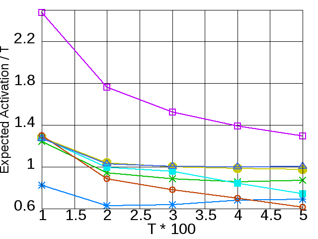
(a) ER, activation

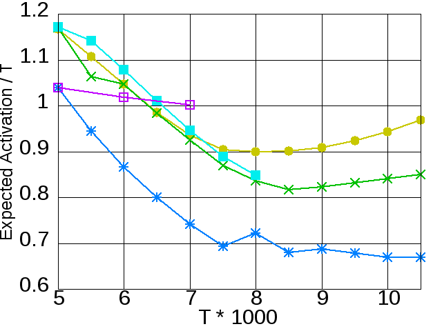
(b) Nethept, activation

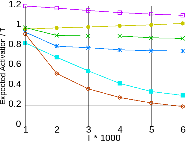
(c) Youtube, activation

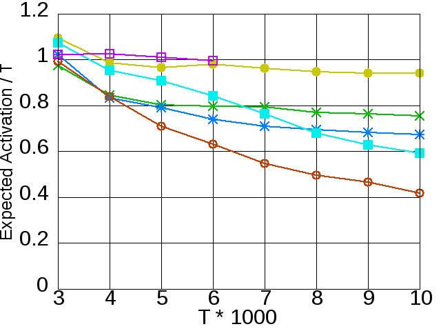
(d) Wikitalk, activation

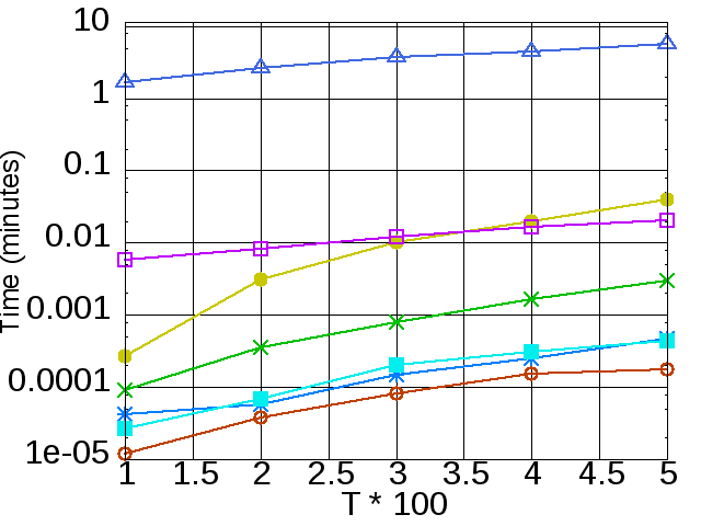
(e) ER, running time

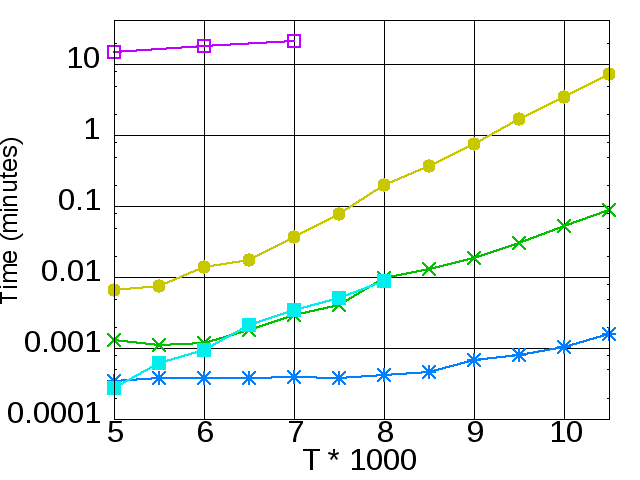
(f) Nethept, running time

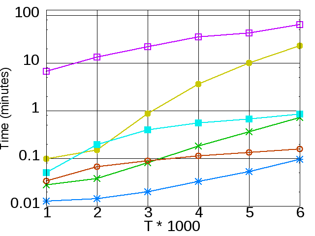
(g) Youtube, running time

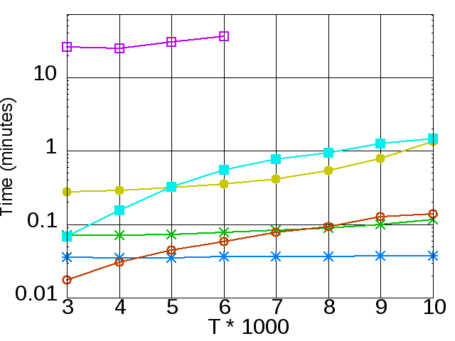
(h) Wikitalk, running time

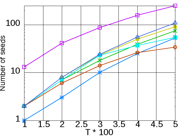
(i) ER, number of seeds

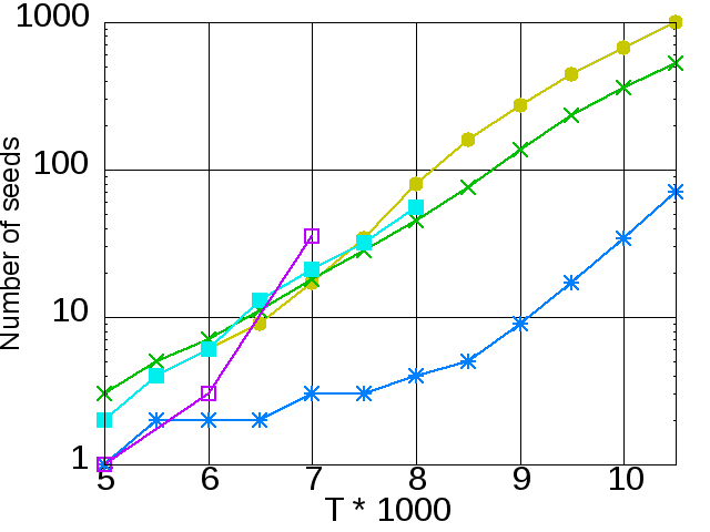
(j) Nethept, number of seeds

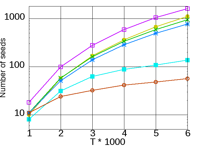
(k) Youtube, number of seeds

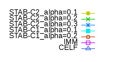
(l) Legend

Figure 1: First row: expected activation normalized by threshold $T$ versus $T$. Second row: running time in minutes versus $T$. Third row: size of seed set versus $T$.

IV-B Performance comparison and demonstration of scalability

In this section, we compare the performance of STAB-C1 and STAB-C2 to CELF and IMM as described above; we experimented on the datasets listed in Table I, where the total CPU time required to compute the oracles is shown. The oracle computation is parallelizable, and in our experiments we used 7 threads of computation. The oracles for each value of $\alpha$ were computed once and stored, and thereafter when running STAB the oracles were simply read from a file. The running times we report for the various versions of STAB do not include the oracle computation time unless otherwise specified. Also in Table I are the values of $ip_{max}$ used for each dataset in this set of experiments. Since IMM and CELF do not consider external influence, the experiments in this section had no external influence; that is, $ep_{max}=0$ for all datasets. To evaluate the seed set returned by the algorithms we used the average activation from 10000 independent Monte Carlo samples.

We show typical results in Fig. 1 on the following four datasets: ER 1000 ($n=1000$), Nethept, Youtube, and Wikitalk. The first row of Fig. 1 shows the expected activation, normalized by the threshold value $T$, of the seed set returned by each algorithm plotted against $T$. Thus, a value of $1$ indicates the algorithm successfully achieved the threshold of activation. The second row of the figure shows the running time in minutes of each algorithm against $T$, and the third row shows the size of the seed set returned by each algorithm.

For the ER 1000 network results are shown in the first column of Fig. 1; this dataset was the only one on which CELF finished under the time limit of 60 minutes. We see that IMM is consistently returning a larger seed set than STAB and CELF and overshooting the threshold value in activation by as much as a factor of 2.5. Thus, it has poor performance of minimizing the size $k$ of the seed set for TAP. This behavior appears to be a result of IMM underestimating the influence of its seed set internally. As expected, CELF performs very well in terms of the size of the seed set and meeting the threshold $T$, but is running on a timescale larger than the other algorithms by factor of at least 100 and as large as $10^{4}$. Notice that STAB-C2 with $\alpha=0.1$ has virtually identical activation and size of seed set to CELF, while running at a much faster speed; as expected, the quality of solution of STAB deteriorates as $\alpha$ is raised, but the running time decreases drastically. In addition, notice that none of the versions of STAB seed too many nodes and overshoot the threshold as IMM does; instead, STAB errs on the side of seeding too few nodes and only partially achieving the threshold $T$ of activation. Finally, it is evident that STAB-C1 runs faster than STAB-C2 and has a similar amount of activation when the seed set required is relatively small. However, the larger the seed set required, the farther is STAB-C1 from achieving the threshold $T$ while STAB-C2 does not suffer from this drawback.

The results from Nethept are shown in the second column of Fig. 1; with $n=15,229$, CELF was unable to run within the time limit, and IMM was able to complete its binary search only for $T\leq 7000$; for the higher threshold values, IMM exceeded the 32 GB memory usage limit imposed in our setup. On this network, STAB-C2 again exhibits the best performance. Despite an initial decrease in activation relative to $T$ shown in Fig. 1(b), the trend reverses around $T=8000$ and seed set size $100$ and the algorithm gets closer to achieving the threshold. This behavior is explained by lower coefficient of variation of estimator $C2$ as analyzed in [17]; the CV can be lower than estimator $C1$ by up to a factor of $\sqrt{|A|}$, where $A$ is the seed set. In stark contrast, STAB-C1 was unable to proceed past $T=8000$ even for $\alpha=0.1$ because the estimator $C1$ appears to lose accuracy as the number of seeds increases. By this mechanism, STAB-C1 had achieved its maximum estimation of influence of any set and thereby could not increase it before reaching an estimated activation of $T$, for $T>8000$.

Next, the Youtube network is shown in the third column of Fig. 1. As in the ER network, IMM is underestimating the influence of its seed set and thereby picking too many seeds and overshooting the threshold, as shown in Fig. 1(c); IMM picks nearly twice as many seed nodes as STAB-C1, $\alpha=0.1$, as shown in Fig. 1(k). In Fig. 1(g), the scalability of STAB is demonstrated as the most precise version, STAB-C2 with $\alpha=0.1$, runs faster than IMM by as much as a factor of 50. On our largest dataset, the Wikitalk network, IMM again exceeded 32 GB memory after $T=6000$; notice that the running time of STAB in all cases is under 2 minutes and STAB-C2 with $\alpha=0.3$ maintained activation greater than $0.6T$ while running in less than 5 seconds, as shown in Fig. 1(h). With inclusion of the parallelizable and reusable oracle computation time of 122 seconds from Table I, the total time taken by STAB-C2 is less than 3 minutes. The total running time for $\alpha=0.1$ of STAB-C2 including the oracles at $T=10000$ is less than 30 minutes.

Choice of $\alpha$: The above discussion demonstrates that $\alpha=0.1$ provides the close activation to the threshold $T$ while maintaining high scalability. If faster running time is desired, $\alpha$ may be increased, which results in a loss of accuracy shown clearly in Fig. 1(d), for $\alpha\in\{0.1,0.2,0.3\}$. On the other hand, if activation closer to $T$ is required, smaller values of $\alpha$ may be used at higher computational cost.

IV-C External influence

In this section, we analyze the performance of STAB when external influence is present in the network; that is, when $ep_{max}>0$. For this section, we considered a BA network with 100,000 nodes, with a threshold of $T=1000$, and the Facebook network with $T=1500$. Results on other topologies were qualitatively similar. For all experiments in this section, we set $\alpha=0.1$.

In 2(a), we plot the expected activation (Act) of the seed set returned by STAB-C2 normalized by the threshold $T$, as $ep_{max}$ varies from 0 to 0.006. As in the previous section, the expected activation of the returned seed set $A$ is estimated by independent Monte Carlo sampling. We also plot the expected fraction of $T$ activated by the external influence, along with the size of the seed set returned by STAB-C2, normalized by its maximum value. As the effect of external influence in the network increases, the algorithm requires fewer seed nodes to ensure the expected activation is within the specified error tolerance to threshold $T$.

In 2(b), we show an analogous plot for the Facebook network; interestingly, the size of the seed set chosen by STAB-C2 nearly doubles as $ep_{max}$ increase from 0 to 0.01, before beginning to decrease to 0. This increase differs from what we expected; it is counterintuitive that the algorithm would require more seeds to reach the threshold as external influence increases. One possible explanation for this effect is that the external influence both decreases and distributes the marginal gain more evenly among seed nodes, so that the greedy algorithm has a more difficult time identifying the best seed nodes, especially in the presence of the error of estimation.

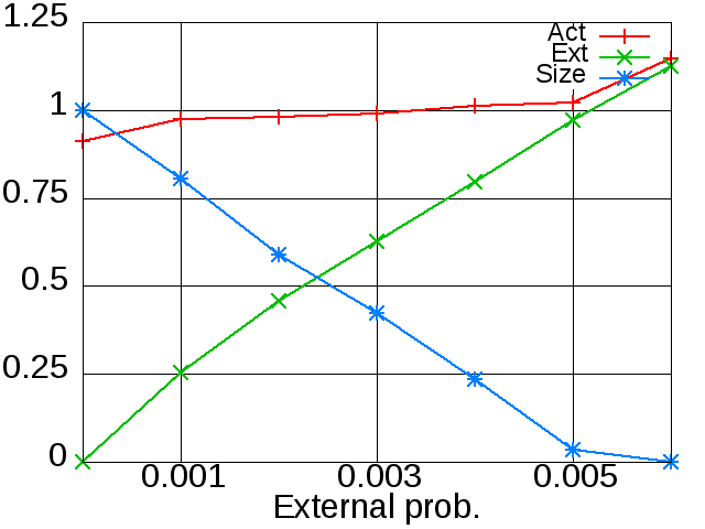
(a) BA 100,000

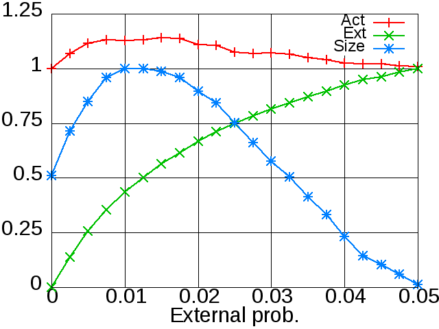
(b) Facebook

Figure 2: The effect of external influence on activation and size of seed set of STAB-C2.

V Related work

Kempe et al. introduced the triggering model in a seminal work on the IM problem [1], where they exhibited a Monte Carlo greedy sampling algorithm that achieves $1-1/e$ performance ratio for IM; this algorithm, although it runs in polynomial time, is very inefficient and cannot scale well. Since the maximum coverage problem prohibits performance guarantee better than $1-1/e+o(1)$ under standard assumptions, the ratio for IM likely cannot be improved, but much work has improved the scalability of the algorithm while retaining the guarantee. Leskovec et al. [19] introduced the CELF method to exploit submodularity and improve the running time. Reverse Influence Sampling (RIS) was introduced in [4] to further improve the greedy performance; algorithms using RIS include [4, 10, 9, 21, 22]; the current state-of-the-art are the SSA [21] and the IMM algorithm [9] to which we compare in this paper. Cohen et al. [3] introduced a methodology for a highly scalable IM algorithm SKIM; in this work, we extend this methodology to solve the TAP problem with the triggering model and external influence.

As compared with IM, much less effort has been devoted to scalable solutions to TAP while maintaining performance guarantees; Goyal et al. [11] studied the TAP problem with monotonic and submodular models of influence propagation; their bicriteria guarantees differ from ours, and provide no method of efficient sampling required for scalability. Chen et al. [23] considered external influence in a viral marketing context. However, their model of external influence is much less general than ours. Furthermore, they restrict external influence to only pass through seed consumers and have no discussion of sampling, scalability, or the TAP problem. Nguyen et al. [24, 25] studied methods to restrain propagation in social networks.

VI Conclusion

We establish equivalency between the triggering model and generalized reachability, which allows incorporation of external influence into our efficient sampling techniques. We gave precise trade-off between accuracy and running time with a bound on the number of samples required to solve TAP. Our algorithm is highly scalable and outperforms adaptations to TAP of the current state-of-the-art algorithm for the IM problem.

References

- [1] David Kempe, Jon Kleinberg, and Éva Tardos. Maximizing the spread of influence through a social network. In Proceedings of the 9th ACM SIGKDD International Conference on Knowledge Discovery and Data Mining, pages 137–146, 2003.
- [2] Thang N Dinh, Huiyuan Zhang, Dzung T Nguyen, and My T Thai. Cost-effective viral marketing for time-critical campaigns in large-scale social networks. IEEE/ACM Transactions on Networking (TON), 22(6):2001–2011, 2014.
- [3] Edith Cohen, Daniel Delling, Thomas Pajor, and Renato F. Werneck. Sketch-based Influence Maximization and Computation: Scaling up with Guarantees. In Proceedings of the 23rd ACM International Conference on Conference on Information and Knowledge Management, pages 629–638, 2014.
- [4] Christian Borgs, Michael Brautbar, Jennifer Chayes, and Brendan Lucier. Maximizing Social Influence in Nearly Optimal Time. In Proceedings of the Twenty-Fifth Annual ACM-SIAM Symposium on Discrete Algorithms, pages 946–957, 2014.
- [5] Huiyuan Zhang, Thang N Dinh, and My T Thai. Maximizing the spread of positive influence in online social networks. In Distributed Computing Systems (ICDCS), 2013 IEEE 33rd International Conference on, pages 317–326. IEEE, 2013.
- [6] Huiyuan Zhang, Dung T Nguyen, Huiling Zhang, and My T Thai. Least cost influence maximization across multiple social networks. IEEE/ACM Transactions on Networking, 24(2):929–939, 2016.
- [7] Thang N Dinh, Dung T Nguyen, and My T Thai. Cheap, easy, and massively effective viral marketing in social networks: truth or fiction? In Proceedings of the 23rd ACM conference on Hypertext and social media, pages 165–174. ACM, 2012.
- [8] Huiyuan Zhang, Huiling Zhang, Alan Kuhnle, and My T Thai. Profit Maximization for Multiple Products in Online Social Networks. In IEEE International Conference on Computer Communications, 2016.
- [9] Youze Tang. Influence Maximization in Near-Linear Time : A Martingale Approach. In Proceedings of the 2015 ACM SIGMOD International Conference on Management of Data, pages 1539–1554, 2015.
- [10] Youze Tang, Xiaokui Xiao, and Yanchen Shi. Influence maximization: Near-optimal time complexity meets practical efficiency. In Proceedings of the 2014 ACM SIGMOD International Conference on Mangement of Data, pages 75–86, 2014.
- [11] Amit Goyal, Francesco Bonchi, Laks V S Lakshmanan, and Suresh Venkatasubramanian. On minimizing budget and time in influence propagation over social networks. Social Network Analysis and Mining, 3(2):179–192, 2013.
- [12] Sharad Goel, Ashton Anderson, Jake Hofman, and Duncan J Watts. The Structural Virality of Online Diffusion. Management Science, 62(1):180–196, 2016.
- [13] Sandra González-Bailón, Javier Borge-Holthoefer, and Yamir Moreno. Broadcasters and Hidden Influentials in Online Protest Diffusion. American Behavioral Scientist, 57:943–965, 2013.
- [14] Seth A. Myers and Jure Leskovec. The bursty dynamics of the Twitter information network. In Proceedings of the 23rd International Conference on World Wide Web, pages 913–924, 2014.
- [15] Seth A. Myers, Chenguang Zhu, and Jure Leskovec. Information diffusion and external influence in networks. In Proceedings of the 18th ACM SIGKDD International Conference on Knowledge Discovery and Data Mining, pages 33–41, 2012.
- [16] Edith Cohen. Size-Estimation Framework with Applications to Transitive Closure and Reachability. Journal of Computer and System Sciences, 55(3):441–453, 1997.
- [17] Edith Cohen, H Kaplan, and Tel Aviv. Leveraging discarded samples for tighter estimation of multiple-set aggregates. ACM SIGMETRICS Performance Evaluation Review, 37(1):251–262, 2009.
- [18] Wei Chen, Chi Wang, and Yajun Wang. Scalable influence maximization for prevalent viral marketing in large-scale social networks. In Proceedings of the 16th ACM SIGKDD International Conference on Knowledge Discovery and Data Mining, pages 1029–1038, 2010.
- [19] Jure Leskovec, Andreas Krause, Carlos Guestrin, Christos Faloutsos, Jeanne VanBriesen, and Natalie Glance. Cost-effective Outbreak Detection in Networks. In Proceedings of the 13th ACM SIGKDD international conference on Knowledge discovery and data mining, pages 420–429, 2007.
- [20] Jure Leskovec and Andrej Krevl. SNAP Datasets: Stanford large network dataset collection. http://snap.stanford.edu/data, June 2014.
- [21] H.T. Nguyen, M. T. Thai, and T. N. Dinh. Stop-and-Stare: Optimal Sampling Algorithms for Viral Marketing in Billion-Scale Networks. In ACM SIGMOD/POSD Conference, 2016.
- [22] H. T. Nguyen, T. N. Dinh, and M. T. Thai. Cost-aware Targeted Viral Marketing in Billion-scale Networks. In IEEE International Conference on Computer Communications, 2016.
- [23] Wei Chen, Fu Li, Tian Lin, and Aviad Rubinstein. Combining Traditional Marketing and Viral Marketing with Amphibious Influence Maximization. In Proceedings of the 16th ACM Conference on Economics and Computation, pages 779–796, 2015.
- [24] N. P. Nguyen, Y. Xuan, and M. T. Thai. A novel method for worm containment on dynamic social networks. In Military Communications Conference, pages 2180–2185, 2010.
- [25] Nam P. Nguyen, T. N. Dinh, D. T. Nguyen, and M. T. Thai. Overlapping community structures and their detection on social networks. In Privacy, Security, Risk, and Trust (PASSAT) and 2011 Third International Conference on Social Computing, 2011.