Deep-learning Top Taggers or The End of QCD?

Abstract

Machine learning based on convolutional neural networks can be used to study jet images from the LHC. Top tagging in fat jets offers a well-defined framework to establish our DeepTop approach and compare its performance to QCD-based top taggers. We first optimize a network architecture to identify top quarks in Monte Carlo simulations of the Standard Model production channel. Using standard fat jets we then compare its performance to a multivariate QCD-based top tagger. We find that both approaches lead to comparable performance, establishing convolutional networks as a promising new approach for multivariate hypothesis-based top tagging.

1 Introduction

Geometrically large, so-called fat jets have proven to be an exciting as well as useful new analysis direction for many LHC Run I and Run II analyses. Their jet substructure allows us to search for hadronic decays for example of Higgs bosons bdrs , weak gauge bosons w_tag , or top quarks early_top ; hopkins ; template ; heptop1 ; heptop2 ; shower_deco in a shower evolution otherwise described by QCD radiation tagging_review . Given this success, a straightforward question to ask is whether we can analyze the same jet substructure patterns without relying on advanced QCD algorithms. An example of such an approach are wavelets, describing patterns of hadronic weak boson decays wavelet_tim ; wavelet_monk . Even more generally, we can apply image recognition techniques to the two-dimensional azimuthal angle vs rapidity plane, for example searching for hadronic decays of weak bosons slac1 ; slac2 ; irvine_w ; gan or top quarks ann_top . The same techniques can be applied to separate quark-like and gluon-like jets quark_gluon .

Many of the available machine learning applications in jet physics have in common that we do not have an established, well-performing QCD approach to compare to. Instead, machine learning techniques are motivated by their potential to actually make such analyses possible. Our study focuses on the question of how machine learning compares to state-of-the-art top taggers in a well-defined fat jet environment, i. e. highly successful QCD-based tagging approaches established at the LHC. Such a study allows us to answer the question if QCD-based taggers have a future in hadron collider physics at all, or if they should and will eventually be replaced with simple pattern recognition.

On the machine learning side we will use algorithms known as convolutional neural networks convnet . Such deep learning techniques are routinely used in computer vision, targeting image or face recognition, as well as in natural language processing. In jet physics the basic idea is to view the azimuthal angle vs rapidity plane with calorimeter entries as a sparsely filled image, where the filled pixels correspond to the calorimeter cells with non-zero energy deposits and the pixel intensities to the deposited energy. After some image pre-processing, a training sample of signal and background images can be fed through a convolutional network, designed to learn the signal-like and background-like features of these jet images slac2 ; quark_gluon . The final layer of the network converts the learned features of the image into a probability of it being either signal or background. The performance can be expressed in terms of its receiver operator characteristic (ROC), in complete analogy to multivariate top tagger analyses heptop3 ; heptop4 .

1.1 Multivariate analysis tools

Top tagging is a typical (binary) classification problem. Given a set of variables $\{x_{i}\}$ we predict a signal or background label $y$. In general, we train a classifier on a data set with known labels and then test the performance of the classifier on a different data set.

Rectangular cuts are sufficient if the variables $x_{i}$ contain orthogonal information and the signal region variable space is simply connected. A decision tree as a classifier is especially useful if there are several disconnected signal regions, or if the shape of the signal region is not a simple box. The classification is based on a sequence of cuts to separate signal from background events, where each criterion depends on the previous decision. Boosting sequentially trains a collection of decision trees, where in each step the training data is reweighted according to the result of the previous classifier. The final classification of the boosted decision tree (BDT) is based on the vote of all classifiers, and leads to an increased performance and more stable results. BDTs are part of the standard LHC toolbox, including modern top taggers heptop4 . We will use them for the QCD-based taggers in our comparison.

Artificial Neural Networks (ANN) mimic sets of connected neurons. Each neuron (node) combines its inputs linearly, including biases, and yields an output based on a non-linear activation function. The usual implementation are feed-forward networks, where the input for a node is given by a subset of the outputs of the nodes in the previous layer. Here, nodes in the first layer work on the $\{x_{i}\}$, and the last layer performs the classification. The internal layers are referred to as hidden layers. The internal parameters of a network, i. e. the weights and biases of the nodes, are obtained by minimizing a so-called cost or loss function. Artificial networks with more than one or two hidden layers are referred to as deep neural networks (DNN). ANNs and DNNs are frequently used in LHC analyses dnn .

In image and pattern recognition convolutional networks (ConvNets) have shown impressive results. Their main feature is the structure of the input, where for example in a two-dimensional image the information of neighboring pixels should be correlated. If we attempt to extract features in the image with standard DNN and fully connected neurons in each layer to all pixels, the construction scales poorly with the dimensionality of the image. Alternatively, we can first convolute the pixels with linear kernels or filters. The convoluted images are referred to as feature maps. On all pixels of the feature map we can apply a non-linear activation function, such that the feature maps serve as input for further convolution layers, where the kernels mix information from all input feature maps. After the last convolution step, the pixels of the feature maps are fed to a standard DNN. While the convolution layers allow for the identification of features in the image, the actual classification is performed by the DNN. While an arbitrarily large non-convolutional DNN should be able to learn features in the image directly, the convolution layers lead to much faster convergence of the model. Image recognition in terms of ConvNets has only recently been tested for LHC applications slac2 ; quark_gluon . The machine learning side of our comparison will be based on ConvNets.

1.2 Image recognition

Image recognition includes many operations, which we will briefly review in this section. The convolutional neural network starts from a two-dimensional input image and identifying characteristic patterns using a stack of convolutional layers. We use a set of standard operations, starting from the $n\times n$ image input $I$:

• ZeroPadding: $(n\times n)\to(n+2\times n+2)$
  We artificially increase the image by adding zeros at all boundaries in order to remove dependence on non-trivial boundary conditions,

  $$I\to\begin{pmatrix}0&\cdots&0\\ \vdots&I&\vdots\\ 0&\cdots&0\end{pmatrix}\;.$$ (1)

• Convolution: $n^{\prime}_{\text{c-kernel}}\times(n\times n)\to n_{\text{c-kernel}}\times((n-n_{\text{c-size}}+1)\times(n-n_{\text{c-size}}+1))$
  To identify features in an $n\times n$ image or feature map we linearly convolute the input with $n_{\text{c-kernel}}$ kernels of size $n_{\text{c-size}}\times n_{\text{c-size}}$. If in the previous step there are $n^{\prime}_{\text{c-kernel}}>1$ layers, the kernels are moved over all input layers. For each kernel this defines a feature map $\widetilde{F}^{k}$ which mixes information from all input layers

  $$\widetilde{F}^{k}_{ij}=\sum_{l=0}^{n^{\prime}_{\text{c-kernel}}-1}\quad\sum_{r,s=0}^{n_{\text{c-size}}-1}\widetilde{W}^{kl}_{rs}\;I^{l}_{i+r,j+s}+b_{k}\qquad\text{for}\quad k=0,...,n_{\text{c-kernel}}-1\;.$$ (2)

• Activation: $(n\times n)\to(n\times n)$
  This non-linear element allows us to create more complex features. A common choice is the rectified linear activation function (ReLU) which sets pixel with negative values to zero, $f_{\text{act}}(x)=\max(0,x)$. In this case we define for example

  $$F^{k}_{ij}=f_{\text{act}}(\widetilde{F}^{k}_{ij})=\max\left(0,\widetilde{F}^{k}_{ij}\right)\;.$$ (3)

  Instead of introducing an additional unit performing the activation, it can also be considered as part of the previous layer.

• Pooling: $(n\times n)\to(n/p\times n/p)$
  We can reduce the size of the feature map by dividing the input into patches of fixed size $p\times p$ (sub-sampling) and assign a single value to each patch

  $$F^{\prime}_{ij}=f_{\text{pool}}(F_{(ip\dots(i+1)p-1,jp\dots(j+1)p-1})\;.$$ (4)

  MaxPooling returns the maximum value of the subsample $f_{\text{pool}}(F)=\max_{\text{patch}}(F_{ij})$.

A convolutional layer consists of a ZeroPadding, Convolution, and Activation step each. We then combine $n_{\text{c-layer}}$ of these layers, followed by a pooling step, into a block. Each of our $n_{\text{c-block}}$ blocks therefore works with essentially the same size of the feature maps, while the pooling step between the blocks strongly reduces the size of the feature maps. This ConvNet setup efficiently identifies structures in two-dimensional jet images, encoded in a set of kernels $W$ transforming the original picture into a feature map. In a second step of our analysis the ConvNet output constitutes the input of a fully connected DNN, which translates the feature map into an output label $y$:

• Flattening: $(n\times n)\to(n^{2}\times 1)$
  While the ConvNet uses two-dimensional inputs and produces a set of corresponding feature maps, the actual classification is done by a DNN in one dimension. The transition between the formats reads

  $$x=\left(F_{11},\dots,F_{1n},\dots,F_{n1},\dots,F_{nn}\right)\;.$$ (5)

• Fully connected (dense) layers: $n^{2}\to n_{\text{d-node}}$
  The output of a standard DNN is the weighted sum of all inputs, including a bias, passed through an activation function. Using rectified linear activation it reads

  $$y_{i}=\max\left(0,\sum_{j=0}^{n^{2}-1}W_{ij}x_{j}+b_{i}\right)\;.$$ (6)

  For the last layer we apply a specific SoftMax activation function

  $$y_{i}=\frac{\exp\left(W_{ij}x_{j}+b_{i}\right)}{\sum_{i}\exp\left(W_{ij}x_{j}+b_{i}\right)}\;.$$ (7)

  It ensures $y_{i}\in[0,1]$, so the label can be interpreted as a signal or background probability.

In a third step we define a cost or loss function, which we use to train our network to a training data set. For a fixed architecture a parameter point $\theta$ is given by the ConvNet weights $\widetilde{W}_{rs}^{kl}$ defined in Eq.(2) combined with the DNN weights $W_{ij}$ and biases $b_{i}$ defined in Eq.(6). We minimize the the mean squared error

$$L(\theta)=\frac{1}{N}\sum_{i=0}^{N}\left(y(\theta;x_{i})-y_{i}\right)^{2}\;,$$ (8)

where $y(\theta;x_{i})$ is the predicted binary label of the input $x_{i}$ and $y_{i}$ is its true value. This choice of loss function does not optimize the learning performance or the probabalistic information, but it will work fine for our purpose. Eventually, it could for example be replaced by the cross entropy. For a given parameter point $\theta$ we compute the gradient of the loss function $L(\theta)$ and first shift the parameter point from $\theta_{n}$ to $\theta_{n+1}$ in the direction of the gradient $\nabla L(\theta_{n})$. In addition, we can include the direction of the previous change such that the combined shift in parameter space is

$$\theta_{n+1}=\theta_{n}-\eta_{L}\nabla L(\theta_{n})+\alpha(\theta_{n}-\theta_{n-1})\;.$$ (9)

The learning rate $\eta_{L}$ determines the step size and can be chosen to decay with each step (decay rate). The parameter $\alpha$, referred to as momentum, dampens the effect of rapidly changing gradients and improves convergence. The Nesterov algorithm changes the point of evaluation of the gradient to

$$\theta_{n+1}=\theta_{n}-\eta_{L}\nabla L(\theta_{n}+\alpha(\theta_{n}-\theta_{n-1}))+\alpha(\theta_{n}-\theta_{n-1})\;.$$ (10)

Each training step (epoch) uses the full set of training events.

2 Machine learning setup

The goal of our analysis is to determine if a machine learning approach to top tagging at the LHC offers a significant advantage over the established QCD-based taggers, and to understand the learning pattern of such a convolutional network. To reliably answer this question we build a flexible neural network setup, define an appropriate interface with LHC data through the jet images, and optimize the ConvNet/DNN architecture and parameters for top tagging in fat jets. To build our neural network we use the Python package Theano theano , with a Keras front-end keras . An optimized speed or CPU usage is not part of our performance study.

2.1 Jet images and pre-processing

The basis of our study are calorimeter images, which we produce using standard Monte Carlo simulations — obviously, in an actual application they should come from data. In recent years, many strategies have been developed to define appropriate signal samples which allow us to benchmark top taggers. Typically, they rely on top pair production with an identified leptonic top decay recoiling against a top jet. The lepton kinematics can then be used to estimate the transverse momentum of the hadronically decaying top quark. We simulate a 14 TeV LHC hadronic $t\bar{t}$ sample and a QCD dijet sample with Pythia8 pythia , ignoring multiple interactions. While one could clearly include pile-up in the simulations, understanding and removing it requires information beyond the calorimeter images, for examples from tracks. For our early study we do not include track information in our jet image, some ideas in this direction are pointed out in Ref. quark_gluon

All events are passed through a fast detector simulation with Delphes3 delphes with calorimeter towers of size $\Delta\eta\times\Delta\phi=0.1\times 5^{\circ}$ and a threshold of 1 GeV. We cluster these towers with FastJet3 fastjet to $R=1.5$ anti-$k_{T}$ anti_kt jets with $|\eta|<1.0$. These anti-$k_{T}$ jets give us a smooth outer shape of the fat jet and a well-defined jet area for our jet image. To ensure that the jet substructure in the jet image is consistent with QCD we re-cluster the anti-$k_{T}$ jet constituents with an $R=1.5$ C/A jet ca_algo . Its substructures define the actual jet image. When we identify calorimeter towers with pixels of the jet image, it is not clear whether the information should be the energy $E$ or only its transverse component $E_{T}$.

Our fat jets have to fulfill $|\eta_{\text{fat}}|<1.0$, to guarantee that they are entirely in the central part of the detector and to justify our calorimeter tower size. For this paper we focus on the range $p_{T,\text{fat}}=350~{}...~{}450$ GeV, such that all top decay products can be easily captured in the fat jet. For signal events, we require that the fat jet can be associated with a Monte-Carlo truth top quark within $\Delta R<1.2$.

Figure 1: Jet image after pre-processing for the signal (left) and background (right). Each picture is averaged over 10,000 actual images.

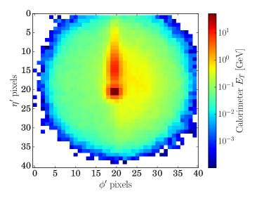
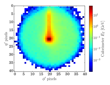
We can speed up the learning process or illustrate the ConvNet performance by applying a set of pre-processing steps:

1. Find maxima: before we can align any image we have to identify characteristic points. Using a filter of size $3\times 3$ pixels, we localize the three leading maxima in the image;

2. Shift: we then shift the image to center the global maximum taking into account the periodicity in the azimuthal angle direction;

3. Rotation: next, we rotate the image such that the second maximum is in the 12 o’clock position. The interpolation is done linearly;

4. Flip: next we flip the image to ensure the third maximum is in the right half-plane;

5. Crop: finally, we crop the image to $40\times 40$ pixels.

Throughout the paper we will apply two pre-processing setups: for minimal pre-processing we apply steps 1, 2 and 5 to define a centered jet image of given size. Alternatively, for full pre-processing we apply all five steps. In figure 1 we show averaged signal and background images based on the transverse energy from 10,000 individual images after full pre-processing. The leading subjet is in the center of the image, the second subjet is in the 12 o’clock position, and a third subjet from the top decay is smeared over the right half of the signal images. These images indicate that fully pre-processed images might lose a small amount of information at the end of the 12 o’clock axis.

Figure 2: Effect of the preprocessing on the image mass calculated from $E$-(left) and $E_{T}$-images (right) of signal (top) and background(bottom). The right set of plots illustrates the situation for forward jets with $|\eta|>2$.

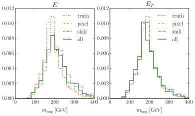
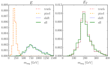
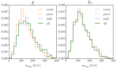
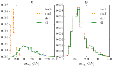
A non-trivial pre-processing step is the shift in the $\eta$ direction, since the jet energy $E$ is not invariant under a longitudinal boost. Following Ref. slac2 we investigate the effect on the mass information contained in the images,

$$m_{\text{img}}^{2}=\left[\sum_{i}E_{i}\left(1,\ \frac{\cos\phi^{\prime}_{i}}{\cosh\eta^{\prime}_{i}},\ \frac{\sin\phi^{\prime}_{i}}{\cosh\eta^{\prime}_{i}},\frac{\sinh\eta^{\prime}_{i}}{\cosh\eta^{\prime}_{i}}\right)\right]^{2}\qquad E_{i}=E_{T,i}\cosh\eta^{\prime}_{i}\;,$$ (11)

where $\eta^{\prime}_{i}$ and $\phi^{\prime}_{i}$ are the center of the $i$th pixel after pre-processing. The study of all pre-processing steps and their effect on the image mass in figure 2 illustrates that indeed the rapidity shift has the largest effect on the $E$ images, but this effect is not large. For the $E_{T}$ images the jet mass distribution is unaffected by the shift pre-processing step. The reason why our effect on the $E$ images is much milder than the one observed in Ref. slac2 is our condition $|\eta_{\text{fat}}|<1$. In the the lower panels of figure 2 we illustrate the effect of pre-processing on fat jets with $|\eta|>2$, where the image masses changes dramatically. Independent of these details we use pre-processed $E_{T}$ images as our machine learning input convnet ; sklearn ; keras ; theano . Since networks prefer small numbers, we scale the images to keep most pixel entries between 0 and 1.

2.2 Network architecture

Figure 3: Left: performance of some of our tested architectures for full pre-processing in terms of an ROC curve, including the default DeepTop network. Right: discrimination power or predicted signal probability for signal events and background probability for background events. We use the default network.

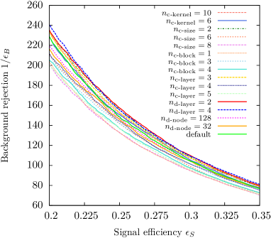
To identify a suitable DeepTop network architecture, we scan over several possible realizations or hyper-parameters. As discussed in the last section, we start with jet images of size $40\times 40$. For architecture testing we split our total signal and background samples of 600,000 images each into three sub-samples: training (150,000 signal and background events each), validation/optimization (150,000 signal and background events each), and final test (300,000 signal and background events each). Networks are trained on the training sample. No early stopping is performed, but the set of weights minimizing loss on the validation/optimization sample is used to avoid overfitting.

In a first step we need to optimize our network architecture. The ConvNet side is organized in $n_{\text{c-block}}$ blocks, each containing $n_{\text{c-layer}}$ sequences of ZeroPadding, Convolution and Activation steps. For activation we choose the ReLU step function while weights are initialized by drawing from a Glorot uniform distribution glorot . Inside each block the size of the feature maps can be slightly reduced due to boundary effects. For each convolution we globally set a filter size or convolutional size $n_{\text{c-size}}\times n_{\text{c-size}}$. The global number of kernels of corresponding feature maps is given by $n_{\text{c-kernel}}$. Two blocks are separated by a pooling step, in our case using MaxPooling, which significantly reduces the size of the feature maps. For a quadratic pool size of $p\times p$ fitting into the $n\times n$ size of each feature map, the initial size of the new block’s input feature maps is $n/p\times n/p$. The final output feature maps are used as input to a DNN with $n_{\text{d-layer}}$ fully connected layers and $n_{\text{d-node}}$ nodes per layer.

hyper-parameter	scan range	default
$n_{\text{c-block}}$	1,2,3,4	2
$n_{\text{c-layer}}$	2,3,4,5	2
$n_{\text{c-kernel}}$	6,8,10	8
$n_{\text{c-size}}$	2,4,6,8	4
$n_{\text{d-layer}}$	2,3,4	3
$n_{\text{d-nodes}}$	32,64,128	64
$p$	0,2,4	2

Table 1: Range of parameters defining the combined ConvNet and DNN architecture, leading to the range of efficiencies shown in the left panel of figure 3 for fully pre-processed images.

Figure 4: Architecture draw_convnet of our default networks for fully pre-processed images, defined in Tab. 1.

In the left panel of figure 3 we show the performance of some test architectures. We give the complete list of tested hyper-parameters in Tab. 1. As our default we choose one of the best-performing networks on the validation/optimization sample after explicitly ensuring its stability with respect to changing its hyper-parameters. The hyper-parameters of the default network we use for fully as well as minimally pre-processed images are given in Tab. 1. In figure 4 we illustrate this default architecture.

Figure 5: Averaged signal minus background for our default network and full pre-processing. The rows correspond to ConvNet layers one to four. After two rows MaxPooling reduces the number of pixels by roughly a factor of four. The columns indicate the feature maps one to eight. Red areas indicate signal-like regions, blue areas indicate background-like regions.

Figure 6: Averaged signal minus background for our default network and full pre-processing. The rows show the three dense DNN layers. Red areas indicate signal-like regions, blue areas indicate background-like regions.

In the second step we train each network architecture using the mean squared error as loss function and a the Nesterov algorithm with an initial learning rate $\eta_{L}=0.003$ and no momentum. Training is performed on mini-batches with a size of 1000 images per batch. We train our default setup over up to 1000 epochs and use the network configuration minimizing the loss function calculated on the validation/optimization sample. Different learning parameters were used to ensure convergence when training on the minimally pre-processed and the scale-smeared samples. Because the DNN output is a signal and background probability, the minimum signal probability required for signal classification is a parameter that allows to link the signal efficiency $\epsilon_{S}$ with the mis-tagging rate of background events $\epsilon_{B}$.

In section 3 we will use this trained network to test the performance in terms of ROC curves, correlating the signal efficiency and the mis-tagging rate.

Before we move to the performance study, we can get a feeling for what is happening inside the trained ConvNet by looking at the output of the different layers in the case of fully pre-processed images. In figure 5 we show the difference of the averaged output for 100 signal and 100 background images. For each of those two categories, we require a classifier output of at least 0.8. Each row illustrates the output of a convolutional layer. Signal-like red areas are typical for jet images originating from top decays; blue areas are typical for backgrounds. The first layer seems to consistently capture a well-separated second subjet, and some kernels of the later layers seem to capture the third signal subjet in the right half-plane. While one should keep in mind that there is no one-to-one correspondence between the location in feature maps of later layers and the pixels in the input image, we will discuss these kinds of structures in the jet image below.

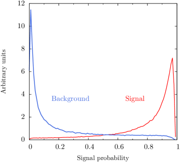
In figure 6 we show the same kind of intermediate result for the two fully connected DNN layers. Each of the 64 linear bars represents a node of the layer. We see that individual nodes are quite distinctive for signal and background images, but they cannot be linked to any pattern in the jet image. This illustrates how the two-dimensional ConvNet approach is more promising that a regular neural net. The fact that some nodes are not discriminative indicates that in the interest of speed the number of nodes could be reduced slightly. The output of the DNN is essentially the same as the probabilities shown in the right panel of figure 3, ignoring the central probability range between 20% and 80%.

Figure 7: Pearson correlation coefficient for 10,000 signal and background images each. The corresponding jet image is illustrated in figure 1. Red areas indicate signal-like regions, blue areas indicate background-like regions.

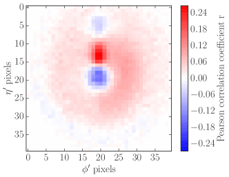
To see which pixels of the fully pre-processed $40\times 40$ jet image have an impact on the signal vs background label, we can correlate the deviation of a pixel $x_{ij}$ from its mean value $\bar{x}_{ij}$ with the deviation of the label $y$ from its mean value $\bar{y}$. A properly normalized correlation function for a given set of combined signal and background images can be defined as

$$r_{ij}=\frac{\sum_{\text{images}}\left(x_{ij}-\bar{x}_{ij}\right)\left(y-\bar{y}\right)}{\sqrt{\sum_{\text{images}}\left(x_{ij}-\bar{x}_{ij}\right)^{2}}\sqrt{\sum_{\text{images}}\left(y-\bar{y}\right)^{2}}}\;.$$ (12)

It is usually referred to as the Pearson correlation coefficient. From the definition we see that for a signal probability $y$ positive values of $r_{ij}$ indicate signal-like patterns. In figure 7 we show this correlation for our network architecture. A large energy deposition in the center leads to classification as background. A secondary energy deposition in the 12 o’clock position combined with additional energy deposits in the right half-plane lead to a classification as signal. This is consistent with our expectations after full pre-processing, shown in figure 1.

3 Performance test

Given our optimized machine learning setup introduced in section 2 and the fact that we can understand its workings and trust its outcome, we can now compare its performance with state-of-the-art top taggers. The details of the signal and background samples and jet images are discussed in section 2.1; essentially, we attempt to separate a top decay inside a fat jet from a QCD fat jet including fast detector simulation and for the transverse momentum range $p_{T,\text{fat}}=350~{}...~{}450$ GeV. Other transverse momentum ranges for the fat jet can be targeted using the same DNN method.

Because we focus on a comparing the performance of the DNN approach with the performance of standard multivariate top taggers we take our Monte Carlo training and testing sample as a replacement of actual data. This distinguishes our approach from tagging methods which use Monte Carlo simulations for training, like the Template Tagger template . This means that for our performance test we do not have to include uncertainties in our Pythia simulations compared to other Monte Carlo simulations and data aussies .

3.1 QCD-based taggers

Acting on the same calorimeter entries in the rapidity vs azimuthal angle plane which define the jet image, we can employ QCD-based algorithms to determine the origin of a given configuration. Based on QCD jet algorithms, for example the multivariate HEPTopTagger2 heptop1 ; heptop2 ; heptop3 ; heptop4 extracts hard substructures using a mass drop condition bdrs

$$\max(m_{1},m_{2})>f_{\text{drop}}\;m_{1+2}$$ (13)

with a given $f_{\text{drop}}=0.8$. Provided that at least three hard substructures exist, different constraints on the invariant masses of combinations of filtered substructures bdrs define a top tag. One of the features of the HEPTopTagger is that even in the multivariate analysis it will always identify a top candidate with a three-prong decay and the correct reconstructed top mass. An alternative approach is to groom the fat jet using the SoftDrop criterion softdrop

$$\frac{\min(p_{T1},p_{T2})}{p_{T1}+p_{T2}}>z_{\text{cut}}\left(\frac{\Delta R_{12}}{R_{0}}\right)^{\beta}$$ (14)

and employ the groomed jet mass. It can be thought of a combination of $p_{T}$-drop criterion hopkins with a soft-collinear extension of pruning pruning . We use the SoftDrop parameters $\beta=1$ and $z_{\text{cut}}=0.2$. The main difference between the HEPTopTagger and SoftDrop is that the latter does not explicitly target the top and $W$ decays, needs an additional condition on a mass scale to work as a tagger, and will not reconstruct the top 4-momentum. Because of these much weaker constraints on the top candidate kinematics a SoftDrop construction is ideally suited for a hypothesis test differentiating between fat QCD jets and top decay jets.

The QCD shower-based taggers alone are known to not fully use the available calorimeter information. However, they can be complemented by a simple observable quantifying the number of constituents inside the fat jet or the number of prongs in the top decay. Adding the $N$-subjettiness nsubjettiness variables

$$\tau_{N}=\frac{1}{R_{0}\sum_{k}p_{T,k}}\sum_{k}p_{T,k}\;\min\left(\Delta R_{1,k},\Delta R_{2,k},\cdots,\Delta R_{N,k}\right)^{\beta}\;.$$ (15)

to the HEPTopTagger or SoftDrop picks up this additional information and also induces the three-prong top decay structure into SoftDrop. We use $N$ $k_{T}$-axes, $\beta=1$ and the reference distance $R_{0}$. A small value $\tau_{N}$ indicates consistency with $N$ or less substructure axes, so an $N$-prong decays give rise to a small ratio $\tau_{N}/\tau_{N-1}$. For top tagging $\tau_{3}/\tau_{2}$ is particularly useful in combination with QCD taggers in a multivariate setup heptop4 . The $N$-subjettiness variables $\tau_{j}$ can be defined based on the complete fat jet or based on the fat jet after applying the SoftDrop criterion. Using $\tau_{j}$ and $\tau^{\text{sd}}_{j}$ in a multivariate analysis usually leads to optimal result.

3.2 Comparison

To benchmark the performance of our DeepTop DNN, we compare its ROC curve with standard Boosted Decision Trees based on the C/A jets using SoftDrop combined with $N$-subjettiness. From figure 3 we know the spread of performance for the different network architectures for fully pre-processed images. In figure 8 we see that minimal pre-processing actually leads to slightly better results, because the combination or rotation and cropping described in section 2.1 leads to a small loss in information. Altogether, the band of different machine learning results indicates how large the spread of performance will be whenever for example binning issues in $p_{T,\text{fat}}$ are taken into account, in which case we we would no longer be using the perfect network for each fat jet.

Figure 8: Performance of the neural network tagger compared to the QCD-based approaches SoftDrop plus $N$-subjettiness and including the HEPTopTagger variables.

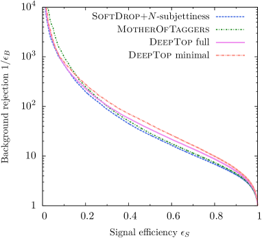
For our BDT we use GradientBoost in the Python package sklearn sklearn with 200 trees, a maximum depth of 2, a learning rate of 0.1, and a sub-sampling fraction of $90\%$ for the kinematic variables

$$\{\ m_{\text{sd}},m_{\text{fat}},\tau_{2},\tau_{3},\tau_{2}^{\text{sd}},\tau_{3}^{\text{sd}}\ \}\qquad\qquad\qquad\text{({SoftDrop} + $N$-subjettiness)}\;,$$ (16)

where $m_{\text{fat}}$ is the un-groomed mass of the fat jet. This is similar to standard experimental approaches for our transverse momentum range $p_{T,\text{fat}}=350~{}...~{}400$ GeV. In addition, we include the HEPTopTagger2 information from filtering combined with a mass drop criterion,

$$\{\ m_{\text{sd}},m_{\text{fat}},m_{\text{rec}},f_{\text{rec}},\Delta R_{\text{opt}},\tau_{2},\tau_{3},\tau_{2}^{\text{sd}},\tau_{3}^{\text{sd}}\ \}\qquad\qquad\qquad\text{({MotherOfTaggers})}\;.$$ (17)

In figure 8 we compare these two QCD-based approaches with our best neural networks. Firstly, we see that both QCD-based BDT analyses and the two neural network setups are close in performance. Indeed, adding HEPTopTagger information slightly improves the SoftDrop+$N$-subjettiness setup, reflecting the fact that our transverse momentum range is close to the low-boost scenario where one should rely on the better-performing HEPTopTagger. Second, we see that the difference between the two pre-processing scenarios is in the same range as the difference between the different approaches. Running the DeepTop framework over signal samples with a 2-prong $W^{\prime}$ decay to two jets with $m_{W^{\prime}}=m_{t}$ and over signal samples with a shifted value of $m_{t}$ we have confirmed that the neural network setup learns both, the number of decay subjets and the mass scale.

Figure 9: Kinematics observables $m_{\text{fat}}$ and $\tau_{3}/\tau_{2}$ for events correctly determined to be signal or background by the DeepTop neural network and by the MotherOfTaggers BDT, as well as Monte Carlo truth.

Following up on on the observation that the neural network and the QCD-based taggers show similar performance in tagging a boosted top decay inside a fat jet, we can check what kind of information is used in this distinction.

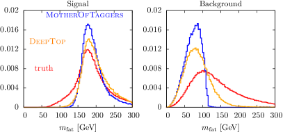
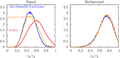
Both for the DNN and for the MotherOfTaggers BDT output we can study signal-like learned patterns in actual signal events by cutting on the output label $y$ corresponding to the 30% most signal like events shown on the right of figure 3. Similarly, we can require the 30% most background like events to test if the background patterns are learned correctly. In addition, we can compare the kinematic distributions in both cases to the Monte Carlo truth. In figure 9 we show the distributions for $m_{\text{fat}}$ and $\tau_{3}/\tau_{2}$, both part the set of observables defined in Eq.(17). We see that the DNN and BDT tagger indeed learn essentially the same structures. The fact that their results are more pronounced signal-like than the Monte Carlo truth is linked to our stiff cut on $y$, which for the DNN and BDT tagger cases removes events where the signal kinematic features is less pronounced. The MotherOfTaggers curves for the signal are more peaked than the DeepTop curves is due to the fact that the observables are exactly the basis choice of the BDT, while for the neural network they are derived quantities. In App. A we extend this comparison to more kinematic observables.

Finally, a relevant question is to what degree the information used by the neural network is dominated by low-$p_{T}$ effects. We can apply a cutoff, for example including only pixels with a transverse energy deposition $E_{T}>5$ GeV. This is the typical energy scale where the DNN performance starts to degrade, as we discuss in more detail in App. B.

4 Conclusions

Fat jets which can include the decay products of a boosted, hadronically decaying top quark are an excellent basis to establish machine learning based on fat jet images and compare their performance to QCD-based top taggers. Here, machine learning is the logical next step after developing multivariate top taggers which test QCD vs top decay hypotheses rather than identifying and reconstructing an actual top decay. This includes the assumption that our ConvNet DeepTop approach will be trained purely on data.

We have constructed a ConvNet setup, inspired by standard image recognition techniques slac2 ; quark_gluon . To optimize the network architecture, train the network, and test the performance we have used independent event samples. First, we have found that changes in the network architecture only have a small impact on the top tagging performance. Pre-processing the fat jet images is useful to visualize, understand, and follow the network learning procedure for example using the Pearson correlation coefficient, but has little influence on the network performance.

As a base line we have constructed a MotherOfTaggers QCD-based top tagger, implemented as a multivariate BDT. This allowed us to quantify the performance of the DeepTop network and to test which kinematic observables in the fat jet have been learned by the neural network. We have also confirmed that the neural network is not dominated by low-$p_{T}$ calorimeter entries and extraordinarily stable with respect to changing the jet energy scale. In figure 8 we found that the performance of the two approaches is comparable, giving us all the freedom to define future experimental strategies for top tagging, ranging from proper top reconstruction to multivariate hypothesis testing and, finally, data-based machine learning.

Appendix A What the machine learns

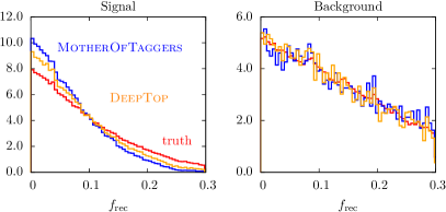
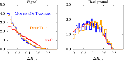
For our performance comparison of the QCD-based tagger approach and the neural network it is crucial that we understand what the DeepTop network learns in terms of physics variables. The relevant jet substructure observables differentiating between QCD jets and top jets are those which which we evaluate in the MotherOfTaggers BDT, Eq.(17).

To quantify which signal features the DNN and the BDT tagger have correctly extracted we show observables for signal event correctly identified as such, i. e. requiring events with a classifier response $y$ corresponding to the 30% most signal like events. Following figure 3 this cut value captures a large fraction of correctly identified events. The same we also do for the $30\%$ most background like events identified by each classifier.

Figure 10: Kinematics observables defined in Eq.(17) for events correctly determined to be signal or background by the DeepTop neural network and by the MotherOfTaggers BDT, as well as Monte Carlo truth. Extended version of figure 9.

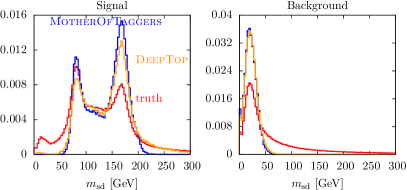
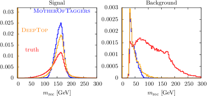
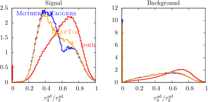
The upper two rows in figure 10 show the different mass variables describing the fat jet. We see that the DNN and the BDT tagger results are consistent, with a slightly better performance of the BDT tagger for clear signal events. For the background the BDT output is more pronounced as well. The deviation from the true mass for the HEPTopTagger background performance is explained by the fact that many events with no valid top candidate return $m_{\text{rec}}=0$. Aside from generally comforting results we observe a peculiarity: the SoftDrop mass identifies the correct top mass in fewer that half of the correctly identified signal events, while the fat jet mass $m_{\text{fat}}$ does correctly reproduce the top mass. The reason why the SoftDrop mass is nevertheless an excellent tool to identify top decays is that its background distribution peaks at very low values, around $m_{\text{sd}}\approx 20$ GeV. Even for $m_{\text{sd}}\approx m_{W}$ the hypothesis test between top signal and QCD background can clearly identify a massive particle decay.

In the third row we see that the HEPTopTagger $W$-to-top mass ratio $f_{\text{rec}}$ only has little significance for the transverse momentum range studied. For the optimalR variable $\Delta R_{\text{opt}}$ heptop4 the DNN and the BDT tagger again give consistent results. Finally, for the $N$-subjettiness ratio $\tau_{3}/\tau_{2}$ before and after applying the SoftDrop criterion the results are again consistent for the two tagging approaches.

Figure 11: Reconstructed transverse momenta for events correctly determined to be signal or background by the DeepTop neural network and by the MotherOfTaggers BDT, as well as Monte Carlo truth.

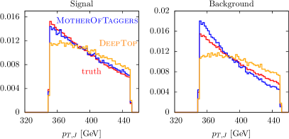
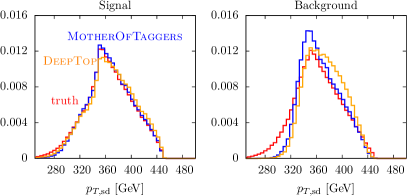
Following up on the observation that SoftDrop shows excellent performance as a hypothesis test, we show in figure 11 the reconstructed transverse momenta of the fat jet, or the top quark for signal events. In the left panel we see that the transverse momentum of the un-groomed fat jet reproduces our Monte-Carlo range $p_{T,\text{fat}}=350~{}...~{}450$ GeV. While the transverse momentum distributions of signal and background are very similar, applying the BDT or DNN induces a bias which indicates a transverse momentum dependent tagger response. The transverse momentum dependence is larger for the DNN. A tagger turn-on with transverse momentum is unproblematic and can be mitigated using adverserial training techniques pivot if needed. In the right panel we see that the constituents identified by the SoftDrop criterion have a significantly altered transverse momentum spectrum. To measure the transverse momentum of the top quark we therefore need to rely on a top identification with SoftDrop, but a top reconstruction based on the (groomed) fat jet properties.

Appendix B Detector effects

Figure 12: Left: Background rejection at a signal efficiency of 30 % for different activation thresholds. Right: Background rejection for the default and hardened training for different re-scalings of the jet images. The background rejection is evaluated at a signal efficiency of 30 % and normalized to the rejection at nominal JES.

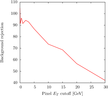
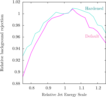
A key question for the tagging performance is the dependence on the activation threshold. Figure. 12 shows the impact of different thresholds on the pixel activation, i. e. $E_{T}$ used both for training and testing the networks. Removing very soft activity, below 3 GeV, only slightly degrades the network’s performance. Above 3 GeV the threshold leads to an approximately linear decrease in background rejection with increasing threshold.

An second, important experimental systematic uncertainty when working with calorimeter images is the jet energy scale (JES). We assess the stability of our network by evaluating the performance on jet images where the $E_{T}$ pixels are globally rescaled by $\pm 25\%$. As shown in the right panel of figure 12 this leads to a decline in the tagging performance of approximately $10\%$ when reducing the JES and $5\%$ when increasing the JES.

Next, we train a hardened version of the network. It uses the same architecture as our default, but during the training procedure each image is randomly rescaled using a Gaussian distribution with a mean of 1.0 and a width of 0.1. New random numbers are used from epoch to epoch. The resulting network has a similar performance as the default and exhibits a further reduced sensitivity to changes in the global JES.

While other distortions of the image, such as non-uniform rescaling, will need to be considered, the resilience of the network and our ability to further harden it are very encouraging for experimental usage where the mitigation and understanding of systematic uncertainties is critical.

References

- (1) J. M. Butterworth, A. R. Davison, M. Rubin and G. P. Salam, Jet substructure as a new Higgs search channel at the LHC, Phys. Rev. Lett. 100, 242001 (2008) [arXiv:0802.2470 [hep-ph]].
- (2) M. H. Seymour, Searches for new particles using cone and cluster jet algorithms: A Comparative study, Z. Phys. C 62, 127 (1994); J. M. Butterworth, B. E. Cox and J. R. Forshaw, scattering at the CERN LHC, Phys. Rev. D 65, 096014 (2002) [arXiv:hep-ph/0201098]; Y. Cui, Z. Han and M. D. Schwartz, W-jet Tagging: Optimizing the Identification of Boosted Hadronically-Decaying W Bosons, Phys. Rev. D 83, 074023 (2011) [arXiv:1012.2077 [hep-ph]].
- (3) W. Skiba and D. Tucker-Smith, Using jet mass to discover vector quarks at the LHC, Phys. Rev. D 75, 115010 (2007) [arXiv:hep-ph/0701247]; B. Holdom, t’ at the LHC: The physics of discovery, JHEP 0703, 063 (2007) [arXiv:hep-ph/0702037]; M. Gerbush, T. J. Khoo, D. J. Phalen, A. Pierce and D. Tucker-Smith, Color-octet scalars at the LHC, Phys. Rev. D 77, 095003 (2008) [arXiv:0710.3133 [hep-ph]].
- (4) D. E. Kaplan, K. Rehermann, M. D. Schwartz and B. Tweedie, Top Tagging: A Method for Identifying Boosted Hadronically Decaying Top Quarks, Phys. Rev. Lett. 101, 142001 (2008) [arXiv:0806.0848 [hep-ph]].
- (5) L. G. Almeida, S. J. Lee, G. Perez, I. Sung and J. Virzi, Top Jets at the LHC, Phys. Rev. D 79, 074012 (2009) [arXiv:0810.0934 [hep-ph]]; L. G. Almeida, S. J. Lee, G. Perez, G. F. Sterman, I. Sung and J. Virzi, Substructure of high- Jets at the LHC, Phys. Rev. D 79, 074017 (2009) [arXiv:0807.0234 [hep-ph]]; L. G. Almeida, S. J. Lee, G. Perez, G. Sterman, I. Sung, Template Overlap Method for Massive Jets, Phys. Rev. D82, 054034 (2010) [arXiv:1006.2035 [hep-ph]]; M. Backovic and J. Juknevich, TemplateTagger v1.0.0: A Template Matching Tool for Jet Substructure, Comput. Phys. Commun. 185, 1322 (2014) [arXiv:1212.2978].
- (6) T. Plehn, G. P. Salam and M. Spannowsky, Fat Jets for a Light Higgs, Phys. Rev. Lett. 104, 111801 (2010) [arXiv:0910.5472 [hep-ph]].
- (7) T. Plehn, M. Spannowsky, M. Takeuchi, and D. Zerwas, Stop Reconstruction with Tagged Tops, JHEP 1010, 078 (2010) [arXiv:1006.2833 [hep-ph]]. http://www.thphys.uni-heidelberg.de/~plehn/index.php?show=heptoptagger&visible=tools
- (8) D. E. Soper and M. Spannowsky, Finding top quarks with shower deconstruction, Phys. Rev. D 87, 054012 (2013) [arXiv:1211.3140 [hep-ph]].
- (9) for a review see e. g. A. Abdesselam et al., Boosted objects: A Probe of beyond the Standard Model physics, Eur. Phys. J. C 71, 1661 (2011) [arXiv:1012.5412 [hep-ph]]; T. Plehn and M. Spannowsky, Top Tagging, J. Phys. G 39, 083001 (2012) [arXiv:1112.4441 [hep-ph]]; A. Altheimer et al., Boosted objects and jet substructure at the LHC, [arXiv:a1311.2708 [hep-ex]]; S. Schaetzel, Boosted Top Quarks and Jet Structure, [arXiv:1403.5176 [hep-ex]].
- (10) V. Rentala, W. Shepherd and T. M. P. Tait, Tagging Boosted Ws with Wavelets, JHEP 1408, 042 (2014) [arXiv:1404.1929 [hep-ph]].
- (11) J. W. Monk, Wavelet Analysis: Event De-noising, Shower Evolution and Jet Substructure Without Jets, [arXiv:1405.5008 [hep-ph]].
- (12) J. Cogan, M. Kagan, E. Strauss and A. Schwarztman, Jet-Images: Computer Vision Inspired Techniques for Jet Tagging, JHEP 1502, 118 (2015) [arXiv:1407.5675 [hep-ph]].
- (13) L. de Oliveira, M. Kagan, L. Mackey, B. Nachman and A. Schwartzman, Jet-images — deep learning edition, JHEP 1607, 069 (2016) [arXiv:1511.05190 [hep-ph]].
- (14) P. Baldi, K. Bauer, C. Eng, P. Sadowski and D. Whiteson, Jet Substructure Classification in High-Energy Physics with Deep Neural Networks, Phys. Rev. D 93, no. 9, 094034 (2016) [arXiv:1603.09349 [hep-ex]].
- (15) L. de Oliveira, M. Paganini and B. Nachman, Learning Particle Physics by Example: Location-Aware Generative Adversarial Networks for Physics Synthesis, [arXiv:1701.0592 [stat.ML]].
- (16) L. G. Almeida, M. Backovic, M. Cliche, S. J. Lee and M. Perelstein, Playing Tag with ANN: Boosted Top Identification with Pattern Recognition, JHEP 1507, 086 (2015) [arXiv:1501.05968 [hep-ph]].
- (17) P. T. Komiske, E. M. Metodiev and M. D. Schwartz, Deep learning in color: towards automated quark/gluon jet discrimination, [arXiv:1612.01551 [hep-ph]].
- (18) see e. g. Y. LeCun, Y. Bengio, and G. Hinton, Geoffrey, Deep learning, Nature 7553, 436 (2015); for nice introductions see e. g. http://www.neuralnetworksanddeeplearning.com or http://www.deeplearning.net
- (19) T. Plehn, M. Spannowsky and M. Takeuchi, How to Improve Top Tagging, Phys. Rev. D 85, 034029 (2012) [arXiv:1111.5034 [hep-ph]]; C. Anders, C. Bernaciak, G. Kasieczka, T. Plehn and T. Schell, Benchmarking an even better top tagger algorithm, Phys. Rev. D 89, no. 7, 074047 (2014) [arXiv:1312.1504 [hep-ph]].
- (20) G. Kasieczka, T. Plehn, T. Schell, T. Strebler and G. P. Salam, Resonance Searches with an Updated Top Tagger, JHEP 1506, 203 (2015) [arXiv:1503.05921 [hep-ph]].
- (21) see e. g. P. Baldi, P. Sadowski and D. Whiteson, Enhanced Higgs Boson to Search with Deep Learning, Phys. Rev. Lett. 114, no. 11, 111801 (2015) [arXiv:1410.3469 [hep-ph]]; J. Searcy, L. Huang, M. A. Pleier and J. Zhu, Determination of the polarization fractions in using a deep machine learning technique, Phys. Rev. D 93, no. 9, 094033 (2016) [arXiv:1510.01691 [hep-ph]]; P. Baldi, K. Cranmer, T. Faucett, P. Sadowski and D. Whiteson, Parameterized neural networks for high-energy physics, Eur. Phys. J. C 76, no. 5, 235 (2016) [arXiv:1601.07913 [hep-ex]]; D. Guest, J. Collado, P. Baldi, S. C. Hsu, G. Urban and D. Whiteson, Jet Flavor Classification in High-Energy Physics with Deep Neural Networks, Phys. Rev. D 94, no. 11, 112002 (2016) [arXiv:1607.08633 [hep-ex]]; R. Santos, J. Webster, S. Ryu, J. Adelman, S. Chekanov and J. Zhou, Machine learning techniques in searches for in the decay channel, [arXiv:1610.03088 [hep-ex]]; A. Alves, Stacking machine learning classifiers to identify Higgs bosons at the LHC, [[arXiv:1612.07725 [hep-ph]].
- (22) Theano Development Team, Theano: A Python framework for fast computation of mathematical expressions, [arXiv:1605.02688 [cs.SC]].
- (23) F. Chollet, https://github.com/fchollet/keras (2015).
- (24) T. Sjöstrand, S. Ask, J. R. Christiansen, R. Corke, N. Desai, P. Ilten, S. Mrenna and S. Prestel et al., An Introduction to PYTHIA 8.2, [arXiv:1410.3012 [hep-ph]].
- (25) J. de Favereau et al. [DELPHES 3 Collaboration], DELPHES 3, A modular framework for fast simulation of a generic collider experiment, JHEP 1402, 057 (2014) [arXiv:1307.6346 [hep-ex]].
- (26) M. Cacciari and G. P. Salam, Dispelling the myth for the jet-finder, Phys. Lett. B 641, 57 (2006) [arXiv:hep-ph/0512210]; M. Cacciari, G. P. Salam and G. Soyez, FastJet User Manual, Eur. Phys. J. C 72, 1896 (2012) [arXiv:1111.6097 [hep-ph]]. http://fastjet.fr
- (27) M. Cacciari, G. P. Salam and G. Soyez, The Anti-k(t) jet clustering algorithm, JHEP 0804, 063 (2008) [arXiv:0802.1189 [hep-ph]].
- (28) Y. L. Dokshitzer, G. D. Leder, S. Moretti and B. R. Webber, Better Jet Clustering Algorithms, JHEP 9708, 001 (1997) [arXiv:hep-ph/9707323]; M. Wobisch and T. Wengler, Hadronization corrections to jet cross sections in deep-inelastic scattering, [arXiv:hep-ph/9907280].
- (29) F. Pedregosa et al., Scikit-learn: Machine Learning in Python, Journal of Machine Learning Research 12, 2825 (2011).
- (30) X. Glorot and Y. Bengio Understanding the difficulty of training deep feedforward neural networks., AISTATS 9 (2010).
- (31) The visualization of the architecture is based on https://github.com/gwding/draw_convnet by G. W. Ding.
- (32) J. Barnard, E. N. Dawe, M. J. Dolan and N. Rajcic, Parton Shower Uncertainties in Jet Substructure Analyses with Deep Neural Networks, [arXiv:1609.00607 [hep-ph]].
- (33) A. J. Larkoski, S. Marzani, G. Soyez and J. Thaler, Soft Drop, JHEP 1405, 146 (2014) [arXiv:1402.2657 [hep-ph]].
- (34) S. D. Ellis, C. K. Vermilion and J. R. Walsh, Techniques for improved heavy particle searches with jet substructure, Phys. Rev. D 80, 051501 (2009) [arXiv:0903.5081 [hep-ph]]; S. D. Ellis, C. K. Vermilion and J. R. Walsh, Recombination Algorithms and Jet Substructure: Pruning as a Tool for Heavy Particle Searches, Phys. Rev. D 81, 094023 (2010) [arXiv:0912.0033 [hep-ph]].
- (35) G. Louppe, M. Kagan, K. Cranmer, Learning to Pivot with Adversarial Networks, Phys. Rev. D 80, 051501 (2009) [arXiv:1611.01046 [stat-ML]]; C. Shimmin, P. Sadowski, P. Baldi, E. Weik, D. Whiteson, E. Goul and A. Søgaard, Decorrelated Jet Substructure Tagging using Adversarial Neural Networks, [arXiv:1703.03507 [hep-ex]].
- (36) J. Thaler and K. Van Tilburg, Identifying Boosted Objects with N-subjettiness, JHEP 1103, 015 (2011) [arXiv:1011.2268 [hep-ph]]; J. Thaler and K. Van Tilburg, Maximizing Boosted Top Identification by Minimizing N-subjettiness, JHEP 1202, 093 (2012) [arXiv:1108.2701 [hep-ph]]; I. W. Stewart, F. J. Tackmann and W. J. Waalewijn, N-Jettiness: An Inclusive Event Shape to Veto Jets, Phys. Rev. Lett. 105, 092002 (2010) [arXiv:1004.2489 [hep-ph]].