Muon $g-2$ and related phenomenology in constrained vector-like extensions of the MSSM

Abstract

We analyze two minimal supersymmetric constrained models with low-energy vector-like matter preserving gauge coupling unification. In one we add to the MSSM spectrum a pair $\mathbf{5}+\mathbf{\bar{5}}$ of $SU(5)$, in the other a pair $\mathbf{10}+\mathbf{\overline{10}}$. We show that the muon $g-2$ anomaly can be explained in these models while retaining perturbativity up to the unification scale, satisfying electroweak and flavor precision tests and current LHC data. We examine also some related phenomenological features of the models, including Higgs mass, fine-tuning, dark matter and several LHC signatures. We stress that, at least for the $\mathbf{5}+\mathbf{\bar{5}}$ model, the parameter space consistent with $g-2$ is entirely in reach of the LHC with a moderate increase in luminosity with respect to the current data set.

1 Introduction

The lack of convincing signals of beyond the Standard Model (BSM) physics at the LHC has severely constrained many scenarios for new physics. More precisely, the idea, mainly motivated by the hierarchy problem, that BSM physics should be found around or just above the electroweak symmetry breaking (EWSB) scale seems to be now under strain in many frameworks, including low scale supersymmetry (SUSY). Direct searches for the sparticles of the Minimal Supersymmetric Standard Model (MSSM) by CMSCMS-PAS-SUS-16-028 ; CMS-PAS-SUS-16-014 ; CMS-PAS-SUS-16-015 ; CMS-PAS-SUS-16-016 and ATLASATLAS-CONF-2016-078 ; ATLAS-CONF-2016-050 ; ATLAS-CONF-2016-054 ; ATLAS-CONF-2016-052 have now pushed the gluino mass bound to 1.7–1.9$\,\mathrm{TeV}$ for most choices of spectrum and decay cascade, each of the light generation squarks to $\sim 1\,\mathrm{TeV}$ and above, and the lightest stop to 700–800$\,\mathrm{GeV}$ and above.

On the other hand, SUSY masses at, or actually above, the 1$\,\mathrm{TeV}$ range show the greatest consistency with the Higgs boson mass at 125$\,\mathrm{GeV}$, especially in models defined at the scale of Grand Unification (GUT) and motivated by supergravity, like the Constrained MSSM (CMSSM) and the Non-Universal Higgs Mass (NUHM) model. In these models the favored parameter space shows sparticles in the range of a few TeV (see, e.g.,Roszkowski:2014wqa ), somewhat decoupled from the EWSB scale, so that all precision observables are expected to yield values in agreement with the Standard Model (SM) within the present experimental sensitivity. As a bonus, one obtains a naturally embedded dark matter (DM) candidate, the lightest neutralino, which can easily satisfy the relic density constraint and yields signatures in reach of present and future direct and indirect DM searches.

By and large precision observables and rare meson decays have been measured in recent years to be in good or even excellent agreement with the SM. However, there exist some long-standing anomalies that point to the existence of BSM physics close to the EWSB scale. The most outstanding and thoroughly studied among them is arguably the anomalous magnetic moment of the muon, $(g-2)_{\mu}$, which shows a deviation from the SM value at more than $3\sigma$Bennett:2006fi ; Miller:2007kk . The anomaly will soon be either confirmed or falsified by the New Muon g-2 experiment at FermilabGrange:2015fou ; Chapelain:2017syu , which is projected to reach a sensitivity of $7\sigma$ to possible BSM effects.

In SUSY, deviations from the SM value of $(g-2)_{\mu}$ are mainly due to the contributions of smuon-neutralino and sneutrino-chargino loops, and require these states to be relatively light. Direct searches for these particles, at LEP first and now at the LHC, constrain them above the few hundred GeV range, but even when recent direct LHC bounds are taken into account, the $(g-2)_{\mu}$ anomaly can be easily explained in the framework of the MSSMEndo:2013bba ; Fowlie:2013oua ; Chakraborti:2014gea ; Das:2014kwa ; Lindner:2016bgg . It is much harder, however, to accommodate the discrepancy in GUT-constrained models. In particular, the bounds from direct squark and gluino searches at the LHC already excludeFowlie:2012im the parameter space that would lead to the correct value of $(g-2)_{\mu}$ in the CMSSM and the NUHM. The simplest, although at the same time the least motivated, way out in such models would be to disunify slepton and squark masses. A more motivated solution is to relax the assumption of a universal gaugino mass, as was shown in, e.g.,Mohanty:2013soa ; Akula:2013ioa ; Chakrabortty:2013voa ; Kowalska:2015zja ; Chakrabortty:2015ika ; Belyaev:2016oxy ; Okada:2016wlm ; Fukuyama:2016mqb .

As an alternative, one can resolve the $(g-2)_{\mu}$ discrepancy by extending the particle content of the MSSM with vector-like (VL) matter, as investigated, e.g., inEndo:2011xq ; Endo:2011mc ; Dermisek:2013gta ; Dermisek:2014cia ; Gogoladze:2015jua ; Aboubrahim:2016xuz ; Nishida:2016lyk ; Higaki:2016yeh ; Megias:2017dzd . The introduction of VL superfields in the superpotential brings along extra degrees of freedom without spoiling the successful unification of gauge interactions at the GUT scaleMartin:2009bg . Extra VL matter, moreover, has been recently considered in the context of several long-standing theoretical issues related to BSM models, and has been shown to be able to provide the effective couplings needed to reconcile some of the other few discrepancies from the SM that have been recently reported by experimental collaborations.

Besides $(g-2)_{\mu}$, it has been for instance pointed out that VL colored sparticles provide extra contributions to the Higgs boson massGraham:2009gy ; Martin:2009bg ; Faroughy:2014oka ; Lalak:2015xea ; Nickel:2015dna ; Barbieri:2016cnt , that VL quarks could possibly explainAngelescu:2015kga the recently emerged $ttH$ anomalyATLAS-CONF-2015-044 , and that VL superfields might ameliorate to some extent the fine tuning associated with large stops with respect to the MSSMDermisek:2016tzw . On the observational side, it has been shown that signatures of extra VL matter can be tested in the next generation of experiments probing lepton flavor violating decaysIbrahim:2015hva , electric and chromoelectric dipole momentsAboubrahim:2015nza ; Aboubrahim:2015zpa , flavor violating Higgs decaysFathy:2016vli and rare meson decays.

In this paper we perform a detailed investigation of $(g-2)_{\mu}$, taking into account the dark matter, Higgs mass, and other constraints in two of the simplest VL extensions of the CMSSM. These are constructed by introducing at the GUT scale either a pair of multiplets in the $\mathbf{5}+\mathbf{\bar{5}}$ representation of $SU(5)$, or a pair $\mathbf{10}+\mathbf{\overline{10}}$ of $SU(5)$. We show that within these frameworks one can manage to maintain a reasonable level of simplicity and be able to explain the $(g-2)_{\mu}$ anomaly. At same time one can retain a good DM candidate without violating any of the constraints from the LHC direct SUSY searches, Higgs measurements, flavor sector, perturbativity in the renormalization group evolution (RGE), and overall consistency with the GUT picture. We provide projections for possible direct signals in the next run of the LHC and we present some comments on issues related to fine tuning, flavor observables, and the $ttH$ anomaly.

The paper is organized as follows. We first present in Sec. 2 the models along with their boundary conditions at the GUT scale. We then focus in Sec. 3 on the low-energy phenomenology of our models and the corresponding bounds on the parameter space. Section 4 presents a detailed description of the mechanisms increasing the value of $(g-2)_{\mu}$ in SUSY models with VL matter and provides analytical formulas for the effect. Finally we show in Sec. 5 our numerical results, and conclude in Sec. 6. The appendices contain more information on the soft SUSY-breaking Lagrangian, the most relevant mass matrices, some useful calculations, and a detailed analysis of the collider constraints.

2 The models

We consider in this work models with new VL fields that are consistent with perturbative gauge coupling unification. The unified models presented here are inspired both by ideas of GUT, based on the $SU(5)$ gauge group, and by expectations of minimality. We therefore do not include additional singlets and focus on simply adding a pair $\mathbf{5}+\mathbf{\bar{5}}$ or a pair $\mathbf{10}+\mathbf{\overline{10}}$ to the MSSM, the VL pair nature of the new fields allowing as usual to give them a superpotential mass. Similarly, we will not suppose any additional discrete symmetry preventing direct mixing between the new fields and the MSSM ones. Finally, let us recall that all of our new fields are charged under lepton number.

In what follows we systematically use small letters for MSSM fields and indicate the $SU(3)\times SU(2)\times U(1)$ quantum numbers in parentheses. With this choice of notation, the MSSM fields are

$$q =(\mathbf{3},\mathbf{2},1/6) H_{u} =(\mathbf{1},\mathbf{2},1/2) l =(\mathbf{1},\mathbf{2},-1/2)$$

$$u =(\mathbf{\bar{3}},\mathbf{1},-2/3) H_{d} =(\mathbf{1},\mathbf{2},-1/2) e =(\mathbf{1},\mathbf{1},1)$$ (1)

$$d =(\mathbf{\bar{3}},\mathbf{1},1/3)\,.$$

The MSSM part of the superpotential is

$$W=\mu\,H_{u}H_{d}-Y_{d}\,qH_{d}d-Y_{e}\,lH_{d}e+Y_{u}\,qH_{u}u\,,$$ (2)

where $\mu$ is the Higgs/higgsino mass parameter, the $Y$ Yukawa couplings are to be understood as $3\times 3$ matrices in flavor space, and we have suppressed generation and isospin indices from the notation.

2.1 The 5-plet LD model

For the first model we consider, which, following the convention ofMartin:2009bg , we refer to as LD, we add to the MSSM spectrum a VL pair $\mathbf{5}+\mathbf{\bar{5}}$ of $SU(5)$, corresponding to the following new fields:

$$D =(\mathbf{\bar{3}},\mathbf{1},1/3) D^{\prime} =(\mathbf{3},\mathbf{1},-1/3)$$

$$L =(\mathbf{1},\mathbf{2},-1/2) L^{\prime} =(\mathbf{1},\mathbf{2},1/2)\,.$$

Hence, with respect to the MSSM, there is one extra quark with charge $-1/3$ (and its antiparticle), one extra charged lepton (and its antiparticle), and 2 extra massive neutrinos. Correspondingly, there are two more squarks, two more sleptons, and two more sneutrinos.

Additional trilinear and bilinear terms are now allowed in the superpotential,

$$W\supset-{\lambda}_{D}\,qH_{d}D-{\lambda}_{L}\,LH_{d}e+M_{D}DD^{\prime}+M_{L}LL^{\prime}+\widetilde{M}_{L}\,lL^{\prime}+\widetilde{M}_{D}\,dD^{\prime}\,,$$ (3)

where the new Yukawa couplings ${\lambda}_{L}$ and ${\lambda}_{D}$ and masses $\widetilde{M}_{L}$ and $\widetilde{M}_{D}$ responsible for the mixing with the SM fields are intended as 3-dimensional arrays spanning the SM generations.

For the fields characterized by the same quantum numbers ($d,D$ and $l,L$) it is possible to choose a basis such that the mixing mass terms are rotated away. This amounts to a redefinition of the other free parameters in the superpotential. However, if this choice is made at the GUT scale, the RGE will in fact regenerate these mixing terms at the SUSY scale. Not including them would therefore amount to tuning the GUT-scale parameters to ensure their subsequent vanishing at the SUSY scale. Since such tuning is not well-motivated and furthermore would break the universality assumption in our boundary conditions, we have chosen to maintain in Eq. (3) the most general form, which includes explicit mass mixing.

The soft SUSY-breaking Lagrangian features additional terms with respect to the MSSM (see Appendix A for the full expression),

$$-\mathcal{L}_{\textrm{soft}} \supset \left[m_{L}^{2}|\tilde{L}|^{2}+m_{L^{\prime}}^{2}|\tilde{L}^{\prime}|^{2}+m_{D}^{2}|\tilde{D}|^{2}+m_{D^{\prime}}^{2}|\tilde{D}^{\prime}|^{2}+\left(\widetilde{m}_{L}^{2}\,\tilde{l}^{{\dagger}}\tilde{L}+\widetilde{m}_{D}^{2}\,\tilde{d}^{{\dagger}}\tilde{D}+\textrm{h.c.}\right)\right]$$ (4)

$$+\left(B_{M_{L}}\tilde{L}\tilde{L}^{\prime}+B_{\widetilde{M}_{L}}\tilde{l}\tilde{L}^{\prime}+B_{M_{D}}\tilde{D}\tilde{D}^{\prime}+B_{\widetilde{M}_{D}}\tilde{d}\tilde{D}^{\prime}+\textrm{h.c.}\right)$$

$$-\left(T_{D}\,\tilde{q}H_{d}\tilde{D}^{{\dagger}}+T_{L}\,\tilde{L}H_{d}\tilde{e}^{{\dagger}}+\textrm{h.c.}\right),$$

where the terms mixing VL and MSSM matter, $\widetilde{m}_{L}^{2}$, $\widetilde{m}_{D}^{2}$, $T_{L}$, $T_{D}$, $B_{\widetilde{M}_{L}}$, and $B_{\widetilde{M}_{D}}$ are, again, to be understood as 3-dimensional arrays.

Since the mixing between the new VL fields and the MSSM ones will be a crucial part of the phenomenology of our model, the explicit form of the fermion and lepton mass matrices will often be very useful. We have therefore included them in Appendix A.

2.2 The 10-plet QUE model

The second model that we consider in this work is obtained by the addition to the MSSM spectrum of a VL pair of fields in a $\mathbf{10}+\mathbf{\overline{10}}$ representation of $SU(5)$. We call it the QUE model. The quantum numbers of the new fields are:

$$Q =(\mathbf{3},\mathbf{2},1/6) Q^{\prime} =(\mathbf{\bar{3}},\mathbf{2},-1/6)$$

$$U =(\mathbf{\bar{3}},\mathbf{1},-2/3) U^{\prime} =(\mathbf{3},\mathbf{1},2/3)$$

$$E =(\mathbf{1},\mathbf{1},1) E^{\prime} =(\mathbf{1},\mathbf{1},-1)\,.$$ (5)

With respect to the MSSM, the $\mathbf{10}+\mathbf{\overline{10}}$ model therefore features two extra quarks with charge $2/3$ (and their antiparticles), one extra quark with charge $-1/3$ and its antiparticle, and one extra lepton with its antiparticle. Correspondingly, there are four extra up-type squarks, two extra down-type squarks and two extra sleptons in the spectrum, with their respective antiparticles.

The additional terms in the superpotential are given by

$$W \supset \lambda_{Qu}\,QH_{u}u-\lambda_{Qd}\,QH_{d}d+\lambda_{U}\,qH_{u}U-\lambda_{E}\,lH_{d}E+Y_{10}\,QH_{u}U-Y_{10}^{\prime}\,Q^{\prime}H_{d}U^{\prime}$$ (6)

$$+M_{Q}QQ^{\prime}+M_{U}UU^{\prime}+M_{E}EE^{\prime}+\widetilde{M}_{Q}\,qQ^{\prime}+\widetilde{M}_{U}\,uU^{\prime}+\widetilde{M}_{E}\,eE^{\prime},$$

where, again, all mixing trilinear and mass terms are understood as 3-dimensional arrays spanning the SM generations.

The additional soft terms and the mass matrices can be obtained in a fashion similar to Eq. (4) and following. We leave their explicit form for Appendix A.

2.3 Boundary conditions

Besides the usual parameters of the CMSSM, ${m_{0}}$, $m_{1/2}$, $A_{0}$, $\tan\beta$, and $\rm{sgn}\,\mu$, in the LD model there will be quantities parameterizing the additional terms given in Eqs. (3) and (4). Since with a greater number of parameters it becomes more likely to miss possibly fine-tuned regions in a numerical scan, we will try to strike a balance between thoroughness and economy, driven also by the expectation that the parameters sharing a common origin at the GUT scale should be unified.

Thus, we introduce a common VL superpotential mass value at the GUT scale, $M_{V}\equiv M_{L}=M_{D}$. We extend the definition of $m_{0}^{2}$ to include the GUT-scale value of $m_{L}^{2}$, $m_{L^{\prime}}^{2}$, $m_{D}^{2}$, $m_{D^{\prime}}^{2}$ in Eq. (4), and we use $A_{0}$ to define $T_{L,D}={\lambda}_{L,D}A_{0}$ at the GUT scale. We also introduce a parameter $B_{0}$ such that, for example, $B_{M_{L}}=B_{0}M_{L}$ at the GUT scale and similarly for all other B terms in Eq. (4).

On the other hand, the flavor structure of the extra terms in the superpotential and soft SUSY-breaking Lagrangian is largely unknown and subject to model-building assumptions. As the scope of this analysis is phenomenological, we refrain from making any specific assumption on the flavor UV completion, but rather focus on reasonably wide regions of the parameter space in agreement with flavor constraints.

To maximize the impact of our choice of parameters on the $(g-2)_{\mu}$ observable, which involves the second generation leptons, and at the same time minimize flavor-changing effects involving the first and third generation we assume that the GUT/Planck scale UV completion defines the following boundary conditions for the extra Yukawa couplings:

$${\lambda}_{L}={\lambda}_{D}=\begin{pmatrix}0\\ \lambda_{5}\\ \epsilon\lambda_{5}\end{pmatrix},$$ (7)

where ${\lambda}_{5}$ is a unified Yukawa coupling, $\epsilon$ is a parameter smaller than 1, and the first generation Yukawa mixing is set to zero for practicity, but is to be rather intended as a parameter small enough to satisfy all bounds from first to second generation conversion in the lepton and quark sectors.

The explicit mass mixing terms in Eqs. (3) and (6) can be rotated away at the GUT scale, but are subsequently generated radiatively (see Footnote 2). This implies that they should feature roughly the same flavor structure as in Eq. (7), with a highly suppressed first genetration mixing, and their size be in the few-GeV range. We will therefore choose $\widetilde{M}_{L}=\widetilde{M}_{D}=(0,\widetilde{M},\alpha\widetilde{M})$, expressed in terms of a unified GUT-scale value $\widetilde{M}$ and a parameter $\alpha$ smaller than 1. As we shall see below, $\widetilde{M}$ is also constrained to the few-GeV range by phenomenological bounds, so that it does not play a significant role in obtaining $(g-2)_{\mu}$ and other relevant signatures.

Conversely, the texture of the soft mass matrices in Eq. (4) does play an important role for the phenomenology. Since these terms are subject to largely the same flavor constraints as the Yukawa couplings that mix VL matter and the MSSM fields we assume that, while their diagonal part is set universally by ${m_{0}}$, as is usually the case in GUT-constrained SUSY models, the off-diagonal mixing terms $\widetilde{m}^{2}_{L,D}$ follow a structure similar to Eq. (7). We also parametrize them as

$$\widetilde{m}_{L}^{2}=\widetilde{m}_{D}^{2}=\begin{pmatrix}0\\ \widetilde{m}^{2}\\ \alpha\widetilde{m}^{2}\end{pmatrix},$$ (8)

in terms of a unified GUT-scale value $\widetilde{m}^{2}$ and the parameter $\alpha$ smaller than 1. We point out as a sidenote that a different treatment of the diagonal and off-diagonal elements of the soft matrices is not unreasonable, but rather typical of flavor models inspired by the Froggatt-Nielsen mechanismFroggatt:1978nt , where the elements of the soft mass matrices are generated proportionally to the difference of the charges assigned to different generations (see, e.g.,Nelson:1997bt ).

We finally adopt similar boundary conditions for the QUE model. We introduce the parameters ${\lambda}_{10}$, $\epsilon$, $\widetilde{M}$, $\widetilde{m}^{2}$, and $\alpha$ as before, so that

$${\lambda}_{Qu(d)}={\lambda}_{U}={\lambda}_{E}=\begin{pmatrix}0\\ \lambda_{10}\\ \epsilon\lambda_{10}\end{pmatrix},$$ (9)

and equations similar to Eq. (8) apply for the mass mixing terms. Additionally, we treat the purely VL Yukawa couplings as unified at the GUT scale, $Y_{10}=Y^{\prime}_{10}$, and we scan this independently.

Even if the boundary conditions outlined above favor mixing between the second generation and the VL particles, in the following sections we will comment on phenomena that involve predominantly third-generation effects, like electroweak (EW) fine tuning, or fits to the $ttH$ anomaly, and that might favor models characterized by boundary conditions different from Eqs. (7) and (9), for example, Yukawa couplings of the form ${\lambda}_{U}=(0,\epsilon{\lambda}_{10},{\lambda}_{10})$.

3 Low energy phenomenology

3.1 Gaugino and scalar mass spectra

The phenomenological properties of GUT-unified SUSY models enriched with VL matter has been investigated, e.g., inMartin:2009bg . We briefly recall here some of the main characteristics, focusing in particular on the differences with the CMSSM. For our numerical results we use the SPhenoporod_spheno_2003 ; porod_spheno_2012 code generated by SARAH (see Refs.staub_sarah_2008 ; staub_automatic_2011 ; staub_superpotential_2010 ; staub_sarah_2013 ; staub_sarah_2014 ). The Higgs pole mass is obtained at 2 loops in the effective potential approach and all other masses are given at one loop. The unified values of gaugino and scalar soft masses are given at $M_{\rm GUT}\approx 10^{16}\,\mathrm{GeV}$ and run down to $M_{\rm SUSY}$, defined as usual as the geometrical mean of the physical stop masses. Typical low-energy spectra are determined by the form of the RGE, which is modified by the presence of extra matter fields.

Particularly consequential are modifications to the running of the gluino mass, which result in a reshaping of the GUT-scale parameter space with respect to the CMSSM. Note that, as the dimension of the VL representation increases, the 1-loop beta function becomes less negative. At 1 loop the gluino beta function, which in the CMSSM is $\beta_{M_{3}}^{\textrm{MSSM}}=-6g_{3}^{2}M_{3}$, is modified in the LD model to $\beta_{M_{3}}^{\textrm{LD}}=-4g_{3}^{2}M_{3}$, which results in a gentler slope when running to low energies. In the QUE model, where one obtains $\beta_{M_{3}}^{\textrm{QUE}}=0$ at one loop, 2-loop effects make the gluino mass actually run to smaller values at low energies.

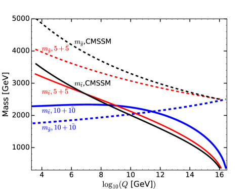
Figure 1: The dashed lines show the running of the gluino soft mass, $M_{3}\approx m_{\tilde{g}}$, in the CMSSM (black), the LD model (red), and the QUE model (blue). The running of the right-chiral stop soft mass, $m_{\tilde{t}}$, is plotted with solid lines in the same color code. We have considered $m_{1/2}=2.5\,\mathrm{TeV},{m_{0}}=600\,\mathrm{GeV}$ and $A_{0}=2.5\,\mathrm{TeV}$ in all cases and set the VL Yukawa couplings to zero. Note that the GUT scale in the LD and QUE models is slightly lower than in the CMSSM.

We illustrate this behavior in Fig. 1, where the 2-loop running of the gluino mass in the CMSSM is indicated with a black dashed line, and is compared to the running of the gluino mass in the LD model (red dashed line), and in the QUE model (blue dashed).

When ${m_{0}}$ is not too large, which is the case of interest for explaining the anomalous magnetic moment of the muon, the running of the gluino mass provides the leading term to the low-scale renormalization of sparticle masses for the color sector and renders their SUSY-scale value not much dependent on the initial choice of ${m_{0}}$. The solid lines in Fig. 1 follow the running of the lightest soft stop mass, $m_{\tilde{t}}$ , in the CMSSM (black), in the LD model (red), and in the QUE model (black). Note that, while in the CMSSM and in the LD model the stops end up being lighter than the gluino at the low scale, in the QUE model they become heavier than the gluino, independently of ${m_{0}}$. As a consequence, given the LHC bounds on the gluino mass, $m_{\tilde{g}}\mathrel{\hbox to0.0pt{\lower 4.0pt\hbox{\hskip 1.0pt$\sim$}\hss}\raise 1.0pt\hbox{$>$}}1.8\,\mathrm{TeV}$, the stops must always be heavier than $\sim 2\,\mathrm{TeV}$ in the QUE model.

More generally, the modifications to the running of gaugino and scalar masses have the effect of shifting the GUT-scale parameter space of models with VL matter to larger values for a given LHC mass bound at the low scale. To give an example, in Fig. 2 we show as a solid red line the current ATLAS 0-lepton direct bound on the mass of squarks and gluinoATLAS-CONF-2016-078 in the CMSSM and the two VL models analyzed in this work. The bound has been recast using the code ofKowalska:2016ent and is shown in the (${m_{0}}$, $m_{1/2}$) plane of the CMSSM in Fig. 2(a) (solid red line). From Figs. 2(b) and 2(c) one can infer that the direct bound bites increasingly into larger GUT-scale parameters in the models with additional matter.

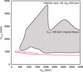
(a)

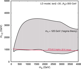
(b)

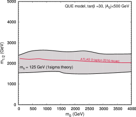
(c)

Figure 2: The red solid line marks the ATLAS 0-lepton search lower boundATLAS-CONF-2016-078 . The region of correct Higgs mass in the (${m_{0}}$, $m_{1/2}$) plane for $\tan\beta\approx 30$ and $|A_{0}|<500\,\mathrm{GeV}$ is shown in pencil gray shaded in: (a) CMSSM, (b) the LD model and (c) the QUE model.

3.2 Higgs sector

As mentioned above, and in some contrast to most previous studies considering the Higgs mass in SUSY theories with new VL matter, in this work we include the 2-loop corrections arising from the new particles (notable exceptions areNickel:2015dna ; Staub:2016dxq ).

Additional VL fields can modify the Higgs pole mass in two ways. First, by adding extra loop corrections. This was thoroughly investigated in Ref.Martin:2009bg , and it was shown there that, in case of a large hierarchy between the fermionic and scalar components of the VL fields, corrections up to 15$\,\mathrm{GeV}$ could be obtained. Second, $m_{h}$ can be modified by altering the MSSM Yukawa couplings (and in particular the top Yukawa) through the mixing of the new VL fields with the MSSM ones.

As already pointed out inMartin:2009bg , the LD model offers small mass improvements compared to the MSSM. Essentially, the largest effect originates from the RGE modifications, which lead to trilinear couplings being typically more negative than in the CMSSM and thereby increase the Higgs mass for equivalent boundary conditions at the GUT scale.

In Fig. 2(b) one can see the region of correct Higgs mass within an assumed $1\sigma\approx 3\,\mathrm{GeV}$ theoretical error in the (${m_{0}}$, $m_{1/2}$) plane of the LD model. It should be compared with the equivalent plane in the CMSSM, Fig. 2(a). We assume in the plots that $\tan\beta\approx 30$ and $|A_{0}|<500\,\mathrm{GeV}$. Note that the region of correct Higgs mass in the LD model is characterized by a slightly smaller size of the GUT-scale soft masses than in the CMSSM. The difference is not, however, very dramatic.

The QUE model differs more from the CMSSM. This is not only because of more substantial modifications to the RGE, but also because of the loop corrections involving the extra Yukawa couplings in Eq. (6), which have the effect of giving a significant increase to the Higgs mass. We give an example of this in Fig. 3, where we show the relative increase (with respect to the CMSSM) of the Higgs mass, $\Delta m_{h}$, in the QUE model, as a function of the SUSY-scale value of ${\lambda}_{U}$ for different choices of $Y_{10}$ at the GUT scale. Note that the curves are obtained for fixed values of ${m_{0}}$, $m_{1/2}$, $A_{0}$, and $\tan\beta$, set as in the QUE benchmark point presented in Sec. 5.1. Note that, in the limit of zero VL Yukawa couplings, there remains a residual Higgs mass difference with the CMSSM which is due to different RGE in both models.

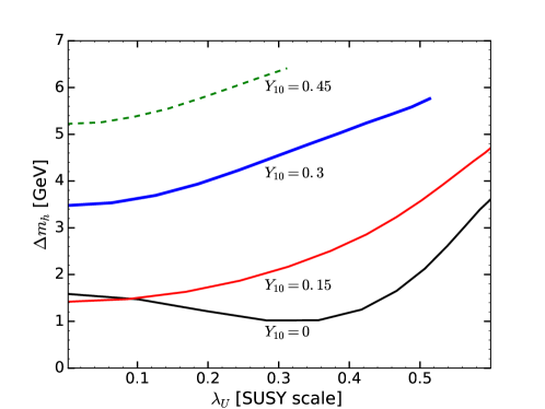
Figure 3: Higgs mass difference in the QUE model with respect to the CMSSM as a function of $\lambda_{U}$ (SUSY scale) for various values of $Y_{10}$ at the GUT scale. From bottom to top $Y_{10}=0,\,0.15,\,0.3,\,0.45$. These values correspond roughly to 0, 0.5, 0.75, and 1 at the SUSY scale. The values of ${m_{0}}$, $m_{1/2}$, $A_{0}$, and $\tan\beta$ are fixed as in the QUE benchmark point, see Sec. 5.1.

As a consequence, in the QUE model one obtains generally a good Higgs mass value in the parameter space that is already being tested at the LHC, as Fig. 2(c) shows. Additionally, as the Higgs mass can easily become too heavy, imposing $m_{h}\approx 125\,\mathrm{GeV}$ often produces an upper bound on the extra Yukawa couplings given a specific choice of $M_{\rm SUSY}$ and $\tan\beta$.

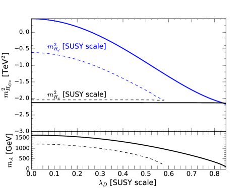
Figure 4: Soft SUSY-breaking masses $m_{H_{u}}^{2}$ and $m_{H_{d}}^{2}$ in the LD model, as well as the pseudoscalar Higgs pole mass $m_{A}$ as a function of the Yukawa coupling $\lambda_{D}$ at the SUSY scale. We fix ${m_{0}}=300\,\mathrm{GeV}$ and $m_{1/2}=1500\,\mathrm{GeV}$. We assume $\tan\beta=10$ for the thick solid lines and $\tan\beta=40$ for the thin dashed lines.

An interesting difference with the CMSSM pertains to the size of the heavy Higgs boson masses in the LD model. The presence of the $D$ superfield in Eq. (3) modifies the running of $m_{H_{d}}^{2}$, as the relative beta function picks up a $6\lambda_{D}^{2}$ contribution, while the RGE for $m_{H_{u}}^{2}$ remains unchanged. We show in Fig. 4 the low scale values of $m_{H_{u}}^{2}$ and $m_{H_{d}}^{2}$ as functions of the $\lambda_{D}$ coupling at the SUSY scale. As the Higgs soft masses increasingly approach each other, the heavy Higgs bosons become lighter (for instance, the tree-level form of the pseudoscalar mass reads $m_{A,\textrm{tree}}\sim|m^{2}_{H_{d}}-m^{2}_{H_{u}}|/\sqrt{1-\sin^{2}2\beta}$).

One of the main consequences of this effect is that, in the LD model, the pseudoscalar mass $m_{A}$ can almost be traded for ${\lambda}_{D}$ as a free parameter, thus opening up additional parameter space when it comes to obtaining the correct DM relic density. We will come back to this point in Sec. 5.2. Note that the same freedom is not seen in the QUE model, as in that case the beta function of both the $m_{H_{d}}^{2}$ and $m_{H_{u}}^{2}$ soft terms are modified by large contributions.

3.3 Fine tuning

It was recently suggested inDermisek:2016tzw , but previously emerged indirectly inMartin:2009bg as well, that the presence of new VL colored particles mixing with the third generation squarks can lead to possible reductions in the fine tuning of the ${m_{0}}$ parameter with respect to the MSSM. This effect is possibly observed particularly in the QUE model, which features some new couplings involving the third generation squarks.

One can, as Ref.Dermisek:2016tzw suggests, suppress the Yukawa interactions between the VL fields and the Higgs sector to effectively decouple the $H_{u}$ superfield from the color fields responsible for setting the SUSY scale. If these Yukawa cuplings are not forbidden by some symmetry, however, one is more likely to see that for selected values of ${\lambda}_{10}$ and $Y_{10}$ additional “focus point” behavior is induced, as for some choices of the new Yukawa couplings the SUSY-scale value of $m_{H_{u}}^{2}$ becomes less sensitive to the initial value, ${m_{0}}$. In this case, then, one has to take into account the fine tuning due to the chosen value of the Yukawas, which can be significant. Note, however, that, as is usually the case in GUT-constrained models, the dominant source of fine tuning comes from the 2-loop effects on the renormalization of $m_{H_{u}}^{2}$ driven by the gluino mass. This implies that the fine tuning is not significantly altered in our models with respect to the CMSSM.

We can calculate $m_{H_{u}}^{2}$ at the low scale as an approximate function of the GUT-scale parameters (in the range ${m_{0}},m_{1/2}\lesssim 3.5\,\mathrm{TeV}$ and $\tan\beta\approx 30$). One finds

$$m_{H_{u}}^{2}(M_{\rm SUSY}) \simeq 0.07\,m_{0}^{2}-0.92\,m_{1/2}^{2}-0.11\,A_{0}^{2}+0.31\,A_{0}m_{1/2}\,\,\textrm{ (CMSSM)}$$ (10)

$$m_{H_{u}}^{2}(M_{\rm SUSY}) \simeq 0.10\,m_{0}^{2}-0.99\,m_{1/2}^{2}-0.11\,A_{0}^{2}+0.35\,A_{0}m_{1/2}\,\,\textrm{ ({\boldmath LD})}$$ (11)

$$m_{H_{u}}^{2}(M_{\rm SUSY}) \simeq 0.18\,m_{0}^{2}-1.02\,m_{1/2}^{2}-0.13\,A_{0}^{2}+0.49\,A_{0}m_{1/2}\,\,\textrm{ ({\boldmath QUE}), }$$ (12)

for zero GUT-scale values of all new Yukawa couplings, and

$$m_{H_{u}}^{2}(M_{\rm SUSY}) \simeq 0.08\,m_{0}^{2}-0.97\,m_{1/2}^{2}-0.14\,A_{0}^{2}+0.32\,A_{0}m_{1/2}\textrm{ ({\boldmath LD})}$$ (13)

$$m_{H_{u}}^{2}(M_{\rm SUSY}) \simeq -1.11\,m_{1/2}^{2}-0.11\,A_{0}^{2}+0.46\,A_{0}m_{1/2}\textrm{ ({\boldmath QUE}),}$$ (14)

for selected GUT-scale values of the Yukawas: ${\lambda}_{5}\approx 0.1$, ${\lambda}_{10}\approx 0.05$, $Y_{10}\approx 0.05$. In all of the models the coefficient regulating the dependence on the unified gaugino mass, $m_{1/2}$, remains of order 1. As a consequence, $m_{1/2}$ and $\mu$ provide the main source of fine tuning, particularly when the constraints from the Higgs mass and LHC direct SUSY searches are taken into account.

We have calculated the fine tuning of our models with SPheno. The program calculates numerically for all input parameters $p_{i}$ the Barbieri-Giudice measureEllis:1986yg ; Barbieri:1987fn ,

$$FT(p_{i})=\left|\frac{\partial\log M_{Z}^{2}}{\partial\log p_{i}}\right|,$$ (15)

where the pole mass $M_{Z}$ is calculated including the 1-loop tadpole corrections to the scalar potential, using the same procedure as inRoss:2017kjc .

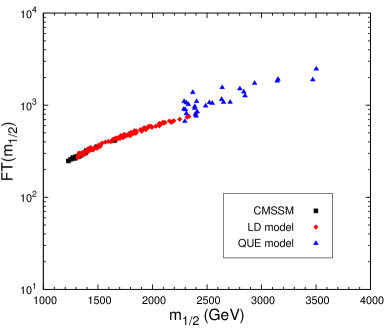
(a)

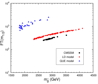
(b)

Figure 5: (a) The tuning of the GUT-scale parameter $m_{1/2}$ as a function of $m_{1/2}$ itself, for the CMSSM (black squares), the LD model (red diamonds), and the QUE model (blue triangles), where we fixed ${m_{0}}\approx 1\,\mathrm{TeV}$ and $|A_{0}|<500\,\mathrm{GeV}$. (b) Same as (a), but as a function of the gluino pole mass $m_{\tilde{g}}$ .

In Fig. 5(a) we show the fine tuning of the LD and QUE models, as a function of $m_{1/2}$, compared to the CMSSM, for a region of the parameter space in agreement with the constraints listed in Sec. 5. The 5-plet model is thus currently tuned at the level of one part in $10^{2}-10^{3}$, not dissimilarly from the CMSSM, whereas the 10-plet model suffers from requiring larger GUT-scale values of the parameters, given an equivalent phenomenology.

We present the dependence on $m_{\tilde{g}}$ in Fig. 5(b), which shows that a given gluino mass leads to a $\sim 50\%$ increase in the tuning of the LD model with respect to the CMSSM, due to a different RGE running. By the same token, the fine tuning associated with the QUE model increases even more drastically, as the physical SUSY masses are there associated with overall larger values of the GUT-scale input parameters.

3.4 Bounds from perturbativity and physicality

Perturbativity is a key requirement that ends up placing constraints on the new Yukawa couplings introduced in Eq. (3) and Eq. (6). A comprehensive study of the infra-red fixed points of the Yukawa couplings of some VL extensions of the MSSM was presented inMartin:2009bg . In this subsection, we limit ourselves to discussing the bounds that apply to our specific models, the 5-plet and the 10-plet.

Note, as a starting point, that the fact that the new Yukawa couplings are fixed at the GUT scale implies that they are always safe from Landau poles. Indeed, as a larger number of Yukawa couplings increase the beta function, choosing one sizable coupling at the GUT scale will simply induce smaller values at the SUSY scale for the other Yukawa couplings. Therefore, the only possible source of non-perturbative behavior are the MSSM Yukawa couplings, which are fixed at the EWSB scale by the experimental value of the fermion masses.

In the LD model, the problematic Yukawa is the one of the bottom quark, $y_{b}$ , as $\lambda_{D}$ and $\lambda_{L}$ introduce only a small contribution to the top Yukawa RGE. Supposing for simplicity that the mixing terms involve the second generation only, ${\lambda}_{D}\equiv{\lambda}_{D,2}$ and ${\lambda}_{L}\equiv{\lambda}_{L,2}$, one has

$$\beta_{y_{b}} \sim y_{b}\Big{(}3|\lambda_{D}|^{2}+|\lambda_{L}|^{2}\Big{)},$$ (16)

which can be used to impose an upper bound on ${\lambda}_{D}$ and ${\lambda}_{L}$. The ratios between the low- and high-scale values of these couplings are approximately ${\lambda}_{D}\approx 1.9\,{\lambda}_{L}\approx 2.3\,{\lambda}_{5}$. From preventing a Landau pole in $y_{b}$ one gets the $\tan\beta$-dependent bound

$${\lambda}_{D}\lesssim\leavevmode\nobreak\ \begin{cases}\leavevmode\nobreak\ 1\qquad\phantom{.7}(\tan\beta=5)\\ \leavevmode\nobreak\ 0.7\qquad(\tan\beta=60)\end{cases}.$$ (17)

In the QUE model, the problematic coupling is the top Yukawa coupling $y_{t}$ , for which new contributions to the beta function read

$$\beta_{y_{t}} \sim-6y_{t}\left(|\lambda_{U,2}|^{2}+2|{\lambda}_{U,3}|^{2}\right)+3{Y_{10}}\left(|\lambda_{U,3}|^{2}+{Y_{10}}y_{t}\right)$$ (18)

in the limit ${\lambda}_{Qu}={\lambda}_{U}$.

When ${\lambda}_{U,3}$ is negligible, we get the bounds

$${\lambda}_{U,2}\lesssim\leavevmode\nobreak\ \begin{cases}\leavevmode\nobreak\ 0.65\qquad(Y_{10}=0.2)\\ \leavevmode\nobreak\ 0.45\qquad(Y_{10}=0.6)\end{cases}.$$ (19)

Conversely, the bounds on ${\lambda}_{U,3}$ are even stronger: ${\lambda}_{U,3}\lesssim 0.45$ with $Y_{10}=0$ and $\widetilde{M}=0$.

Interestingly, however, the bounds on the couplings of the LD model are actually more severe than in Eq. (17), due to the requirement of physical values for the masses of the heavy Higgs bosons, see Sec. 3.2. This, coupled to the requirement that the top Yukawa remains perturbative (which sets a lower bound on $\tan\beta$), yields the bound

$${\lambda}_{D}\lesssim\leavevmode\nobreak\ \begin{cases}\leavevmode\nobreak\ 0.9\qquad(\tan\beta=5)\\ \leavevmode\nobreak\ 0.4\qquad(\tan\beta=60)\end{cases}.$$ (20)

Note that these bounds depend on ${m_{0}}$ : while Eq. (20) has been determined for ${m_{0}}\approx 0.5\,\mathrm{TeV}$, it becomes ${\lambda}_{D}\lesssim\leavevmode\nobreak\ 0.8$ ($0.1$) for $\tan\beta=5$ ($60$) at ${m_{0}}\approx 2.5\,\mathrm{TeV}$.

Comments on $ttH$. We conclude this section with a few comments on the possibility of enhancing the $t\bar{t}h$ production mode in the QUE model, while keeping the gluon-fusion production rate around its measured value, as was suggested inAngelescu:2015kga . Although this possibility remains enticing in generic VL scenarios, the anomaly cannot be explained in models constrained at the GUT scale once all phenomenological bounds are taken into account. In light of the above discussion this is to be expected, as the values for the new Yukawa couplings considered inAngelescu:2015kga are not compatible with our assumption of perturbativity up to the GUT scale.

3.5 Bounds from electroweak precision tests

The mixing between the new VL and the SM leptons is strongly constrained by precision tests of the EW theory. A detailed study of the constraints from these observables is beyond the scope of this paper, but we will derive in this section rough bounds on the parameters relevant in our models. Note that further bounds related to flavor and EW precision tests are directly implemented numerically and will be described in Sec. 5.

We assume for simplicity that only the mixing between the second generation and VL particles is present. The second-lightest charged lepton and neutrino mass eigenstates, $e_{2}$ and $\nu_{2}$, contain a fraction of the VL lepton fields. Their gauge coupling to the $Z$ and $W$ bosons are thus

$$\mathcal{L}\supset Z_{\mu}\bar{e}_{2}\gamma^{\mu}(P_{L}{g^{Z\mu\mu}_{L}}+P_{R}{g^{Z\mu\mu}_{R}})e_{2}+\left[W_{\mu}\bar{\nu}_{2}\gamma^{\mu}P_{L}{g^{W\mu\nu_{\mu}}_{L}}e_{2}+\textrm{h.c.}\right],$$ (21)

where the couplings for our models are given in detail in Appendix B. The absence of a VL left-handed $SU(2)$-singlet in the LD model as well as of a VL right-handed $SU(2)$-doublet in the QUE model limits the corrections to these couplings, as we shall see.

We assume here that the following mass hierarchy holds:

$$m_{\mu}\ll\lambda_{L}v_{d},\lambda_{E}v_{d},\widetilde{M}_{L},\widetilde{M}_{E}\ll M_{L},M_{E}\ .$$ (22)

The most stringent bounds on these parameter originate from two observables. First, the couplings to the $Z$ boson are strongly constrained by the $Z\rightarrow\mu^{+}\mu^{-}$ branching ratio (see, e.g.,Olive:2016xmw ), which imposes a constraint on the modified couplings $\delta g_{L,R}^{Z\mu\mu}\equiv g_{L,R}^{Z\mu\mu}-g_{L,R,\textrm{SM}}^{Z\mu\mu}$ :

$$\frac{\delta{g^{Z\mu\mu}_{L}}}{{g^{Z\mu\mu}_{L,\textrm{SM}}}}\,\,,\,\,\frac{\delta{g^{Z\mu\mu}_{R}}}{{g^{Z\mu\mu}_{L,\textrm{SM}}}}\lesssim 0.1\%\,,$$ (23)

leading to

$$\frac{{\lambda}_{L}v_{d}}{M_{L}}\,\,,\,\,\frac{{\lambda}_{E}v_{d}}{M_{E}}\lesssim 2\%\,.$$ (24)

Second, the measurements of the Fermi constant, using the muon lifetime, constrains the coupling with the $W$ boson (see, e.g.,Dermisek:2015oja ) as

$$\frac{\delta{g^{W\mu\nu_{\mu}}_{L}}}{{g^{W\mu\nu_{\mu}}_{L,\textrm{SM}}}}\,\,,\,\,\frac{\delta{g^{W\mu\nu_{\mu}}_{R}}}{{g^{W\mu\nu_{\mu}}_{R,\textrm{SM}}}}\lesssim 0.05\%\,,$$ (25)

thus producing a stronger bound on the coupling than the direct measurements.

Note, however, that in the LD model these couplings are only generated at order $(\widetilde{M}_{L}/M_{L})^{4}$ in the limit of mixing between the second generation and VL particles only. This leads to a mild constraint $\widetilde{M}_{L}/M_{L}\lesssim 0.1$ (cf. Appendix B). In the QUE model the equivalent constraint is weaker than the one from $\textrm{BR}(Z\rightarrow\mu^{+}\mu^{-})$, Eq. (24).

4 The $(g-2)_{\mu}$ anomaly in VL models

There is a long-standing discrepancy, at the $3\sigma$ or more level, between the value of the anomalous magnetic moment of the muon, $a_{\mu}=(g-2)_{\mu}/2$, measured at BrookhavenBennett:2006fi ; Hagiwara:2011af and the SM expectation.

A recent updateDavier:2016iru of the lowest order hadronic contributions to the calculation of $a_{\mu}$ in the SM places the discrepancy at 

$$\delta\left(g-2\right)_{\mu}\equiv a_{\mu}(\textrm{SM})-a_{\mu}(\textrm{exp})=(27.4\pm 7.6)\times 10^{-10}.$$ (26)

The anomaly, if real, provides a clear hint for new physics not far from the EWSB scale. On the experimental side, the New Muon g-2 experiment at FermilabGrange:2015fou ; Chapelain:2017syu will soon probe the discrepancy at an unprecedented $7\sigma$ level, which is bound to revive the interest of the particle physics community in the subject.

It has been long known that, while the excess can be easily explained in the framework of the MSSM even after the most recent LHC bounds for direct SUSY searches are taken into accountEndo:2013bba ; Fowlie:2013oua ; Chakraborti:2014gea ; Das:2014kwa ; Kowalska:2015zja ; Lindner:2016bgg , the same bounds and the Higgs mass value prevent a good fit in the simplest constrained models, like the CMSSM and the NUHMBechtle:2012zk ; Fowlie:2012im ; Buchmueller:2013rsa . The tension can be ameliorated if one relaxes the assumption of gaugino and/or squark universality, as shown for instance inAkula:2013ioa ; Kowalska:2015zja .

In this section we show that, as an alternative, the tension can be resolved by maintaining universal boundary conditions at the GUT scale, and considering instead additional VL matter, as the new sleptons can contribute to loop corrections and give rise to phenomenological features different from the MSSM. Note that solutions to the $(g-2)_{\mu}$ anomaly employing VL fermions have also been considered inEndo:2011xq ; Endo:2011mc ; Aboubrahim:2016xuz ; Nishida:2016lyk , in general by postulating the existence of a full new generation, which leads to new fermionic contributions in loops involving the $W$ and $Z$ bosons, or in the framework of the MSSM with parameters defined at the SUSY scale.

In the CMSSM-like VL extensions that we consider here we introduce $\mathbf{5}+\mathbf{\bar{5}}$, or $\mathbf{10}+\mathbf{\overline{10}}$ multiplets of $SU(5)$, as described in Sec. 2. The complete one-loop corrections in the mass-eigenstate basis are well-knownMoroi:1995yh ; Martin:2001st and already implemented in many codes, including the SARAH-generated SPheno routines that we use to find the regions of the parameters space that are in agreement with the measured value of $\delta\left(g-2\right)_{\mu}$, the relic abundance, and the other constraints defined in Sec. 5. It is worth, however, first taking a look to the parametric dependence of $\delta\left(g-2\right)_{\mu}$ in our models.

As we explain in more detail in Sec. 5.2, for the neutralino mass range considered here one obtains the correct value of the relic density in the slepton-coannihilation and $A$-funnel regions of the parameter space, which are both characterized by a mostly bino-like neutralino. In the MSSM with bino-like DM, the dominant contributions to $\delta\left(g-2\right)_{\mu}$ are due to the well known neutralino/smuon and chargino/sneutrino loops, and are approximately of comparable strength.

The former, $\Delta a_{\mu}^{\chi^{0}}$, can be expressed, followingMartin:2001st , as a sum over smuon and neutralino mass eigenstates, $\tilde{\mu}_{i}$ and $\chi_{m}^{0}$:

$$\Delta a_{\mu}^{\chi^{0}}\approx\frac{m_{\mu}}{48\,\pi^{2}}\sum_{i,m}\left[\frac{m_{\chi^{0}_{m}}}{m^{2}_{\tilde{\mu}_{i}}}\,\textrm{Re}\left(n_{im}^{L}n_{im}^{R}\right)\mathcal{F}_{N}(x_{im})\right]\,,$$ (27)

where $m_{\mu}$ is the muon mass, the loop function $\mathcal{F}_{N}$ takes the form

$$\mathcal{F}_{N}(x)=\frac{3}{(1-x)^{3}}\left(1-x^{2}+2x\ln x\right),$$ (28)

and $x_{im}\equiv m^{2}_{\chi_{m}^{0}}/m^{2}_{\tilde{\mu}_{i}}$. The effective couplings $n_{im}^{L}$ and $n_{im}^{R}$ parameterize the interaction of the physical smuons with the neutralinos and with left-handed and right-handed muons, respectively. They can be expressed explicitly in terms of the eigenvectors of the neutralino and smuon mass matrices and can be found, e.g., inMartin:2001st .

Equivalently, the dominant chargino/sneutrino contribution, $\Delta a_{\mu}^{\chi^{\pm}}$, readsMartin:2001st

$$\Delta a_{\mu}^{\chi^{\pm}}\approx\frac{m_{\mu}}{24\,\pi^{2}}\sum_{j,k}\left[\frac{m_{\chi^{\pm}_{k}}}{m^{2}_{\tilde{\nu}_{\mu,j}}}\,\textrm{Re}\left(c_{jk}^{L}c_{jk}^{R}\right)\mathcal{F}_{C}(z_{jk})\right]\,,$$ (29)

where the loop function $\mathcal{F}_{C}$ is given by

$$\mathcal{F}_{C}(x)=-\frac{3}{2(1-x)^{3}}\left(3-4x+x^{2}+2\ln x\right),$$ (30)

and $z_{jk}\equiv m^{2}_{\chi_{k}^{\pm}}/m^{2}_{\tilde{\nu}_{\mu,j}}$. Again, $c_{jk}^{L}$ and $c_{jk}^{R}$ are the effective couplings of the physical muon sneutrinos (of which there is one in the MSSM with minimal flavor violation) to the charginos and left-handed and right-handed muons.

In the limit of an almost pure bino LSP – roughly the case for the $A$-funnel region of the CMSSM, but not necessarily for the stau-coannihilation region, in which $\delta\left(g-2\right)_{\mu}$ features non negligible contributions from diagrams involving heavier higgsino-like neutralinos – Eq. (27) takes the simple formMartin:2001st

$$\Delta a_{\mu}^{\chi^{0}}\approx\frac{g_{1}^{2}}{48\pi^{2}}\frac{m_{\mu}^{2}M_{1}(\mu\tan\beta-A_{\mu})}{m_{\tilde{\mu}_{2}}^{2}-m_{\tilde{\mu}_{1}}^{2}}\left[\frac{\mathcal{F}_{N}(x_{11})}{m_{\tilde{\mu}_{1}}^{2}}-\frac{\mathcal{F}_{N}(x_{21})}{m_{\tilde{\mu}_{2}}^{2}}\right],$$ (31)

where the smuon mixing term in the numerator, which depends linearly on $\mu$ and $A_{\mu}$, provides the main source of chirality flip in the loop. Under the same assumptions, the parametric form of Eq. (29) can also be derived (see Appendix C), and reads

$$\Delta a_{\mu}^{\chi^{\pm}}\approx\frac{g_{2}^{2}\,m_{\mu}^{2}}{24\,\pi^{2}}\frac{\mu\,M_{2}\tan\beta}{m_{\chi^{\pm}_{2}}^{2}-m_{\chi^{\pm}_{1}}^{2}}\left[\frac{\mathcal{F}_{C}(z_{11})-\mathcal{F}_{C}(z_{12})}{m_{\tilde{\nu}_{\mu}}^{2}}\right].$$ (32)

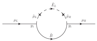
(a)

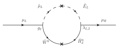
(b)

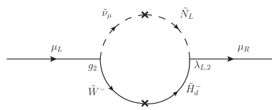
(c)

Figure 6: Main loops contributing to $\delta\left(g-2\right)_{\mu}$ in the LD model. The photon line attached to one of the charged legs is implicit. We have explicitly written the doublet $L$ as $L=(N_{L},E_{L})^{T}$.

The presence of the new VL sector introduces new contributions to $(g-2)_{\mu}$ in two ways, which are summarized for the LD model in Fig. 6:

• There are new sources of smuon mixing, as the second-generation sleptons are mixed with new VL matter, see Fig. 6(a).

• There are new Yukawa couplings, $\lambda_{L}$ and ${\lambda}_{E}$, that are a priori unconstrained and can be much larger than the muon Yukawa, see Figs. 6(b) and 6(c). Note, however, that for models with perturbativity assumed up to the GUT scale the absence of Landau poles does constrain these couplings, see Sec. 3.4.

In the LD model, extra contributions to Eq. (31) are provided by larger mixing between the smuons. The loop correction depicted in Fig. 6(a) modifies Eq. (31) in a non-trivial way, as the smuon mass matrix that must be diagonalized is now $4\times 4$, see Eq. (38) in Appendix A. The physical smuon mixing now depends on the new Yukawa coupling, ${\lambda}_{L}$, and the superpotential and soft-SUSY breaking mixing terms, $\widetilde{M}_{L}$ and $\widetilde{m}^{2}_{L}$.

The loop correction of Fig. 6(c) affects instead the form of the chargino/sneutrino contribution, Eq. (32), which is now modified by an additional term

$$\Delta a_{\mu,\textrm{tot}}^{\chi^{\pm}}=\Delta a_{\mu}^{\chi^{\pm}}+\Delta a_{\mu,\textrm{VL}}^{\chi^{\pm}},$$ (33)

where $\Delta a_{\mu,\textrm{VL}}^{\chi^{\pm}}$ is expressed in terms of the sneutrino mass squared matrix, Eq. (39), and reads (see Appendix C)

$$\Delta a_{\mu,\textrm{VL}}^{\chi^{\pm}}\approx\frac{g_{2}\,m_{\mu}M_{W}}{12\sqrt{2}\,\pi^{2}}\frac{\mu\,M_{2}\sin\beta}{m_{\chi^{\pm}_{2}}^{2}-m_{\chi^{\pm}_{1}}^{2}}\frac{{\lambda}_{L}(M_{L}\widetilde{M}_{L}+\widetilde{m}_{L}^{2})}{m^{2}_{\tilde{\nu}_{\mu,2}}-m^{2}_{\tilde{\nu}_{\mu,1}}}\\ \times\left[\frac{\mathcal{F}_{C}(z_{21})-\mathcal{F}_{C}(z_{22})}{m_{\tilde{\nu}_{\mu,2}}^{2}}-\frac{\mathcal{F}_{C}(z_{11})-\mathcal{F}_{C}(z_{12})}{m_{\tilde{\nu}_{\mu,1}}^{2}}\right].$$ (34)

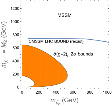
(a)

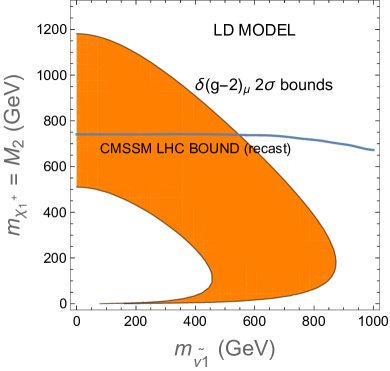
(b)

Figure 7: (a) We show in orange the $2\sigma$ region of $\delta\left(g-2\right)_{\mu}$ from Eq. (32) in the ($m_{\tilde{\nu}_{\mu}}$, $M_{2}$) plane of the MSSM. We assume $\tan\beta=30$ and $\mu=1200\,\mathrm{GeV}$. The LHC lower bound from squark and gluino searchesATLAS-CONF-2016-078 projected to the ($m_{\tilde{\nu}_{\mu}}$, $M_{2}$) plane after CMSSM-like boundary conditions are applied is shown as a solid gray line. (b) The $2\sigma$ region of $\delta\left(g-2\right)_{\mu}$ from Eq. (33) in the ($m_{\tilde{\nu}_{1}}$, $M_{2}$) plane. We assume $M_{L}=600\,\mathrm{GeV}$, ${\lambda}_{L}=0.25$, $\widetilde{M}_{L}=10\,\mathrm{GeV}$, $\widetilde{m}^{2}_{L}=-(500\,\mathrm{GeV})^{2}$, and $m^{2}_{L}\approx m^{2}_{\tilde{\mu}_{L}}$, with all parameters defined at the SUSY scale.

In Fig. 7(a) we derive the approximate $2\sigma$ bounds in the plane of the chargino mass versus muon sneutrino mass of the MSSM, ($m_{\tilde{\nu}_{\mu}}$, $M_{2}$), using the largest contribution, Eq. (32). We superimpose a CMSSM recast of the current LHC bounds from direct squark and gluino searchesATLAS-CONF-2016-078 obtained using the code of Ref.Kowalska:2016ent . The plot confirms that the region of the CMSSM favored by $(g-2)_{\mu}$ data is excluded.

We use Eq. (33) to show in Fig. 7(b) that VL contributions allow one to extend the available parameter space within the $2\sigma$ bounds of $\delta\left(g-2\right)_{\mu}$, so to evade the current LHC limit. Selected values of the VL parameters are given in the caption. Note that the enhanced value with respect to the SM is here due to an entirely supersymmetric effect, unlike the enhancement obtained, e.g., inAboubrahim:2016xuz , which is instead due to loop contributions involving new neutrinos from VL matter belonging to larger representations than the ones considered in this work.

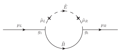
(a)

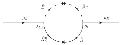
(b)

Figure 8: Main loops contributing to $\delta\left(g-2\right)_{\mu}$ in the QUE model. The photon line attached to one of the charged legs is implicit. We have explicitly written the scalar component of the supermultiplet $E$ as $\tilde{E}$.

Similar considerations apply to the QUE model, with the obvious difference that only neutralino/smuon loops will be enhanced, as there are no extra sneutrinos with respect to the MSSM. The most important contributions due to VL matter are shown in Fig. 8. In particular, the dominant one in the case with bino-like DM, Fig. 8(a), introduces a modification to $\Delta a^{\chi^{0}}_{\mu}$ equivalent to the contribution present in the LD model, where in this case one must use the elements of the mass squared matrix given in Eq. (42).

5 Numerical results

We use MultiNestFeroz:2008xx to direct the scanning procedure and we interface it with various publicly available codes. We use the SARAH-produced SPheno code as our spectrum generator. The flavor related observables are obtained using the SARAH-package FlavorKitPorod:2014xia . Dark matter observables, $\Omega_{\chi}h^{2}$ and $\sigma^{\rm SI}_{p}$, are computed with $\tt micrOMEGAs\ v.3.5.5$Belanger:2013oya . The scan prior ranges we adopt for the parameters of the LD and QUE models are shown in Appendix D.

We build a global likelihood function using the constraints, central values, theoretical and experimental uncertainties shown in Table 1. The Higgs sector is additionally constrained using $\tt HiggsSignals$Bechtle:2013xfa and $\tt HiggsBounds$Bechtle:2008jh ; Bechtle:2011sb ; Bechtle:2013wla . These codes ensure that our Higgs sector is in proper agreement with the most recent LHC bounds, despite possible modifications to the Yukawa couplings that originate from our mixing terms. We also impose a hard cut on $\sigma^{\rm SI}_{p}$ from the latest LUX dataAkerib:2016vxi .

Constraint	Mean	Exp. Error	Th. Error	Ref.
Higgs sector	See text.	See text.	See text.	Bechtle:2013xfa ; Bechtle:2008jh ; Bechtle:2011sb ; Bechtle:2013wla
$\sigma^{\rm SI}_{p}$	See text.	See text.	See text.	Akerib:2016vxi
$\Omega_{\chi}h^{2}$	0.1188	0.0010	10%	Ade:2015xua
$\textrm{BR}\left(\overline{B}\rightarrow X_{s}\gamma\right)\times 10^{4}$	3.32	0.16	0.21	Amhis:2016xyh
$\textrm{BR}\left(B_{u}\rightarrow\tau\nu\right)\times 10^{4}$	0.72	0.27	0.38	Adachi:2012mm
$\Delta M_{B_{s}}$	17.757 ps-1	0.021 ps-1	2.400 ps-1	Olive:2016xmw
$\Delta\rho\times 10^{4}$	$3.7$	$2.3$	$0.5$	Olive:2016xmw
$\textrm{BR}\left(B_{s}\to\mu^{+}\mu^{-}\right)\times 10^{9}$	2.9	$0.7$	10%	Aaij:2013aka ; Chatrchyan:2013bka
$\textrm{BR}\left(\tau^{\pm}\rightarrow\mu^{\pm}\gamma\right)\times 10^{8}$	$<4.4$	$0$	$0$	Aubert:2009ag

Table 1: The experimental constraints included in the likelihood function.

An interesting consequence of the presence in the QUE model of a right-handed VL up-type quark is the possible enhancement of the decay $\textrm{BR}\left(B_{u}\rightarrow\tau\nu\right)$. We have therefore included this observable in the likelihood of our scans. The presence of new down-type VL quarks in both the LD and QUE model can also modify the flavor-changing neutral current $b\rightarrow s$. We have consequently included in the likelihood of our scans the experimental values for $\textrm{BR}\left(\overline{B}\rightarrow X_{s}\gamma\right)$ and $\textrm{BR}\left(B_{s}\to\mu^{+}\mu^{-}\right)$, calculated at one-loop using FlavorKit. We additionally include all the bounds discussed in Sec. 3.

Finally, the constraints from the correction $\Delta\rho$ to the Veltman $\rho$-parameter are calculated at one-loop by SARAH and have been included in the likelihood of our scans.

5.1 Muon g-2 benchmark points

We present in Table 2 benchmark points for the models LD and QUE satisfying all the previous constraints including $\delta\left(g-2\right)_{\mu}$. In the LD benchmark point the muon sneutrino is light thanks to the mixing with the VL sneutrino, and gives the greatest contribution to $\delta\left(g-2\right)_{\mu}$. Conversely, the benchmark point for the QUE model relies on a light slepton to generate a sizable $\delta\left(g-2\right)_{\mu}$. Note the large splitting between the first slepton mass eigenstate (which is mixed smuon/VL) and second slepton eigenstate (which is the usual right-handed stau). Furthermore, as could be inferred in Sec. 4, in order to have a positive contribution to $\delta\left(g-2\right)_{\mu}$ the sign of the new Yukawa couplings and of the new mixing soft terms should preferably be opposite.

	Parameter	LD	QUE
	${m_{0}}$	$600$	$565$
	$m_{1/2}$	$1550$	$2500$
	$A_{0}$	$100$	$2500$
	$M_{V}$	$1000$	$250$
GUT inputs	$B_{0}$	$-\,250$	$0$
	$\lambda_{5}$, $\lambda_{10}$	$0.2$	$0.225$
	$Y_{10}$	–	$0$
	$\widetilde{m}^{2}$	$-1.2\times 10^{6}$	$-6\times 10^{5}$
	$\widetilde{M}$	$2$	$0$
	$\mathrm{tan}\beta$	$40$	$7.5$
	${\lambda}_{D,2}$, ${\lambda}_{U,2}$	$0.47$	$0.59$
	${\lambda}_{Qu,2}$ / ${\lambda}_{Qd,2}$	–	$0.56$ / $0.76$
	${\lambda}_{L,2}$, ${\lambda}_{E,2}$	$0.24$	$0.31$
SUSY scale	$\mu$	$1680$	$3100$
	$B_{\mu}$	$5.5\times 10^{4}$	$1\times 10^{6}$
	$M_{1}$	$546$	$377$
	$M_{2}$	$984$	$633$
	$M_{3}$	$2561$	$1757$
	$M_{D}$, $M_{U}$	$2125$	$810$
	$M_{L}$, $M_{E}$	$1352$	$298$
	$\widetilde{M}_{D,2}$, $\widetilde{M}_{U,3}$	$3.5$	$3.2$
	$m_{h}$	$124.4$	$126.2$
	$m_{A,H}$	$1084$	$2570$
	$m_{\chi_{1}^{0}}$	$539$	$372$
	$m_{\chi^{\pm}_{1}}$	$1013$	$675$
	$m_{\tilde{g}}$	$2700$	$1990$
Pole Masses	$m_{\tilde{e}_{1}}$	$651$	$374$
	$m_{\tilde{e}_{2}}$	$704$	$930$
	$m_{\tilde{\nu}_{1}}$	$710$	$1290$
	$m_{\tilde{t}_{R}}$	$2130$	$2210$
	$m_{E}$	$1370$	$302$
	$m_{B}$	$2260$	$1210$
	$\delta\left(g-2\right)_{\mu}$	$2.2\times 10^{-9}$	$1.8\times 10^{-9}$
Low Energy	$\textrm{BR}\left(B_{u}\rightarrow\tau\nu\right)$	$1.28\times 10^{-4}$	$1.24\times 10^{-4}$
	$\Omega_{\chi}h^{2}$	$0.119$	$0.113$

Table 2: Benchmark points for the models LD and QUE. Dimensionful quantities are given in GeV and $\,\mathrm{GeV}^{2}$, and $\epsilon=\alpha=0$.

The parametric dependence of $\delta\left(g-2\right)_{\mu}$ around the benchmark point of the LD model given in Table 2 is presented in Fig. 9(a). One can easily read out how the size of the observable depends on the new Yukawa couplings and the sneutrino mass. The parametric dependence of $\delta\left(g-2\right)_{\mu}$ around the benchmark point of the QUE model is given in Fig. 9(b).

(a)

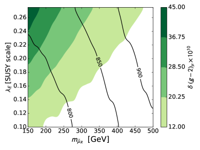
(b)

Figure 9: (a) $\delta\left(g-2\right)_{\mu}$ in the LD model as a function of the pole mass of the first sneutrino eigenstate (a mixed muon sneutrino/VL sneutrino state) and of the Yukawa ${\lambda}_{L}$ at the SUSY scale. The remaining parameters are chosen as in the benchmark point of Table 2. Black lines show contours of the lightest slepton mass. (b) $\delta\left(g-2\right)_{\mu}$ in the QUE model as a function of the pole mass of the first selectron eigenstate (a mixed smuon/ VL slepton state) and of the Yukawa ${\lambda}_{E}$ at the SUSY scale. Black solid lines show contours of the second-lightest slepton mass.

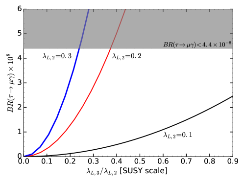
Figure 10: $\textrm{BR}(\tau\rightarrow\mu\gamma)\times 10^{8}$ as function of the ratio $\lambda_{L,3}/\lambda_{L,2}$ at the SUSY scale in the LD model. From top to bottom, the lines correspond to $\lambda_{L,2}\approx 0.3$, 0.2, and 0.1 (which leads to $\delta\left(g-2\right)_{\mu}=12\times 10^{-10},\,18\times 10^{-10}$, and $27\times 10^{-10}$). All other parameters are fixed as in the benchmark point in Table 2.

While in the semi-analytical treatment of the previous sections we have often assumed that the mixing in the Yukawa and soft sectors only involve the second generation and VL particles, the scans include a coupling to the third generation, controlled by a small parameter $\epsilon$. While this parameter is not directly relevant for $\delta\left(g-2\right)_{\mu}$ it will affect for instance the collider phenomenology. The strongest constraint on this parameter comes from the flavor-violating decay, $\textrm{BR}(\tau\rightarrow\mu\gamma)<4.4\times 10^{-8}$. This is illustrated in Fig. 10, where we show the evolution of $BR(\tau\rightarrow\mu\gamma)\times 10^{8}$ as function of the ratio between third and second generation Yukawa couplings.

The QUE model points with a sizable $\delta\left(g-2\right)_{\mu}$ present an interesting compressed spectrum, which can be seen in Table 2. There is a bino-like neutralino, almost degenerate with a mixed smuon/VL slepton and, with mass approximately twice their size, the first chargino. The rest of the spectrum is heavier. A spectrum of this kind is likely to evade LHC bounds due to the degeneracy between the slepton and neutralino, and simultaneously provides the correct relic density (from smuon co-annihilation) and a good $\delta\left(g-2\right)_{\mu}$, as the smuon is relatively light. These interesting properties come however at the expense of an additional fine-tuning in the mass spectrum. We will therefore focus in the rest of the paper on the more promising LD model.

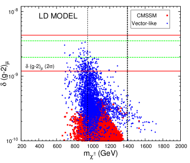
(a)

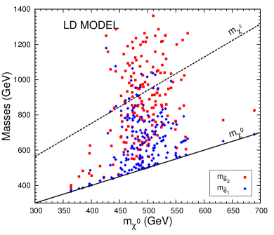
(b)

Figure 11: (a) Comparison of the calculation of $\delta\left(g-2\right)_{\mu}$ for the LD model (blue diamonds) versus the CMSSM (red squares). The horizontal red solid lines indicate the current $\delta\left(g-2\right)_{\mu}$ $2\,\sigma$ region, while the horizontal green dashed ones show the projected $2\,\sigma$ region of the upcoming New Muon g-2 experiment, assuming the measured $\delta\left(g-2\right)_{\mu}$ remains unchanged. The vertical dashed lines show the current (thin) and projected (thick) bounds from 3-lepton searchesATLAS-CONF-2016-096 ; CMS:2016gvu in the simplified-model interpretation. (b) Masses of the two lightest sleptons as function of the neutralino LSP mass. The thin dash line represents the mass of the first chargino.

In Fig. 11(a) we show a plot of $\delta\left(g-2\right)_{\mu}$ versus the lightest chargino mass, $m_{\chi^{\pm}_{1}}$ , for the points of the LD model (blue diamonds). The CMSSM case (red squares) is shown for comparison. One can clearly see the significant enhancement in $\delta\left(g-2\right)_{\mu}$, which now allows one to easily find points that properly fit the experimental anomaly. For the points within $2\sigma$ of the $\delta\left(g-2\right)_{\mu}$ measurement, we show in Fig. 11(b) the mass of the lightest slepton eigenstate (blue diamonds) and of the second slepton mass eigenstate (red squares). All the constraints of Table 1 are satisfied at the $3\sigma$ level in both plots, with the exception of the Higgs mass that is required to be within a $1\sigma\approx 3\,\mathrm{GeV}$ theoretical error. The gluino mass lower boundATLAS-CONF-2016-078 is satisfied for the points in the plot. We have also applied the bounds from direct LHC searches for VL quarks and leptons, which are also satisfied automatically by the points in the plot. The details of the latter bounds, along with corresponding projections for 14$\,\mathrm{TeV}$, 300$\,\text{fb}^{-1}$, are presented in Appendix E.

Because of the frequent presence of light sleptons of mass in between the chargino and the neutralino, the points in the figure are also subject to the most recent constraints from the ATLAS and CMS 3-lepton searches for electroweakino pair productionATLAS-CONF-2016-096 ; CMS:2016gvu . The thin dashed vertical line shows the current limit interpreted in the “flavor-democratic” simplified model with intermediate sleptonsATLAS-CONF-2016-096 . Note that the bound is not to be taken at face value. We postpone a detailed LHC analysis, which requires a full numerical simulation, to future work, but we point out here that we have checked several points characterized by $m_{\chi^{\pm}_{1}}\approx 850\,\mathrm{GeV}$, with an intermediate selectron at about $700\,\mathrm{GeV}$, finding that in many cases the branching fraction of the chargino/neutralino decay chains are different from the simplified model considered by the experimental collaboration (for example, one often finds $\textrm{BR}(\tilde{{\chi}}^{0}_{2}\rightarrow\tilde{\mu}\mu)\approx 50\%$ and $\textrm{BR}(\tilde{{\chi}}^{0}_{2}\rightarrow\tilde{\tau}\tau)\approx 50\%$) so that the efficiency to the 3-lepton final state is reduced. Most of the points shown, even those below 900$\,\mathrm{GeV}$, appear thus to be presently allowed, albeit some of them marginally.

On the other hand, the next round of data with increased luminosity is bound to deeply test the full parameter space that allows for a good $(g-2)_{\mu}$ fit. We report in Fig. 11(a), marked with a thick dashed line, the projected bound from 3-lepton searches in the flavor-democratic scenario at 14$\,\mathrm{TeV}$ and 300$\,\text{fb}^{-1}$, which we take from Ref.Kowalska:2015zja . If the $(g-2)_{\mu}$ anomaly is real there will be unmistakable signatures at the LHC.

Comments of flavor anomalies. We conclude this subsection with some comments on the flavor observables. We have performed a survey of the values of the Wilson coefficients $C_{7}$, $C_{8}$, $C_{9}$, and $C_{10}$ in the LD model. We observe for several points significant deviations from the SM in the coefficients $C_{9}$ and $C_{10}$, which may be useful to partially alleviate the current tensions between the SM predictions and the experimental measurements broadly related to the $b\rightarrow s$ transitions (see, e.g.,Altmannshofer:2014rta ). Indeed global fits for these two coefficients described inAltmannshofer:2014rta ; DescotesGenon:2015uva report best fit points around $(C_{9}^{\textrm{NP}},C_{10}^{\textrm{NP}})\approx(-1.0,0.3)$, with the $2\sigma$ region extending for the former over the range $[-1.5,-0.3]$. A certain number of scan points satisfying the constraints of Table 1 show $C_{9}^{\textrm{NP}}(\approx-0.3C_{10}^{\textrm{NP}})\approx-0.4$, thus being placed within the $2\sigma$ region from global fits. While it is unlikely that our model can explain all of the anomalies, it can reduce the pull compared to the SM. We point out, though, that we do not notice a significant correlation with the region of parameter space that leads to good $\delta\left(g-2\right)_{\mu}$ and for this reason we refrain from further investigating this direction here.

5.2 Dark matter and direct detection

One of the most important phenomenological features of SUSY models is that they provide a natural DM candidate, which is typically the lightest neutralino. The DM relic density plays a crucial role in determining the allowed parameter space of such models since this constraint can be satisfied only if specific conditions characterizing the mass spectrum are met. By adding new VL fields to the model, we can modify the MSSM picture in basically two ways. One is by changing the position of the known regions in the parameter space in which the correct value of the DM relic density can be obtained, e.g., due to modified RGE of the mass parameters from the GUT scale to the EW scale (see, e.g.,Moroi:2011aa ). The other possibility is that new particles appearing in the model will be involved in additional annihilation channels for the lightest neutralino which can even open up new regions of the parameter space (see, e.g.,Abdullah:2015zta ; Abdullah:2016avr ).

As we focus on GUT-constrained scenarios, it is useful to compare our results with the ones obtained for the prototypical model of this kind, the CMSSM (see, e.g.,Roszkowski:2014wqa for an extensive discussion). The correct value of the DM relic density in the CMSSM for the region of the parameter space with bino-like neutralino (we do not treat here the promising region characterized by a higgsino-like neutralino with $\sim 1\,\mathrm{TeV}$ mass, as it requires a roughly SM-like value of $(g-2)_{\mu}$) features either an approximate mass degeneracy between the lightest neutralino and the lightest slepton (slepton coannihilation), or the resonance condition for the $s$-wave pseudoscalar Higgs boson, $A$ ($A$-funnel region).

Both the slepton-coannihilation and $A$-funnel regions are present in the LD and QUE models that we analyze. The slepton-coannihilation region contains both CMSSM-like points characterized by a close mass degeneracy between the neutralino and the lightest stau, as well as points in which the lightest slepton is a mixture of an MSSM-like left chiral smuon and a VL slepton. For the latter points the lightest neutralino is also mass-degenerate with the lightest sneutrino which, being lighter than the lightest charged slepton, can play the dominant role in the coannihilation mechanism responsible for reducing the otherwise too large relic abundance of the bino-like neutralino.

The slepton-coannihilation region in the QUE model is extended to contain points with larger mass difference between the neutralino and the lightest slepton (up to $\sim 160$ GeV) for which the correct value of the DM relic density is achieved partly thanks to coannihilations and partly due to efficient annihilations of the bino-like neutralino into the heavy VL leptons that avoid chirality suppressionAbdullah:2015zta . This effect is less pronounced in the LD model since in the QUE model such annihilations are hypercharge enhanced for weak-isosinglet leptons.

		SC
Region	SC	$+$	AF
		bino ann.
Model	LD / QUE	QUE	LD / QUE
$m_{\chi}$	$469.6$ GeV	$367.8$ GeV	$541.4$ GeV
$m_{\tilde{{\chi}}^{0}_{2}}\simeq m_{\chi^{\pm}_{1}}$	$886$ GeV	$670$ GeV	$1013.7$ GeV
$m_{\widetilde{L}_{1}}^{2}$	$479.6$ GeV	$455.8$ GeV	$992.4$ GeV
$m_{\tilde{\nu}_{1}}$	$470.0$ GeV	$1163.7$ GeV	$988.0$ GeV
$m_{A}$	$1334.3$ GeV	$1543.1$ GeV	$1082.0$ GeV
$\Omega_{\chi}h^{2}$	$0.123$	$0.156$	$0.128$
$\sigma^{\rm SI}_{p}$ [$\textrm{cm}^{2}$]	$1.5\times 10^{-47}$	$3.1\times 10^{-47}$	$1.6\times 10^{-47}$
$\delta\left(g-2\right)_{\mu}$	$2.1\times 10^{-9}$	$1.6\times 10^{-9}$	$1.2\times 10^{-9}$
$m_{h}$	$123.9$ GeV	$123.8$ GeV	$123.1$ GeV

Table 3: Benchmark points for regions with the correct value of the DM relic density: the slepton-coannihilation (SC), $A$-funnel (AF) and a region of slepton-coannihilation with additional efficient bino annihilation into $4th$ generation leptons (SC+bino ann.). The model in which a given region is present in the favored parameter space is also denoted. In case of regions present in both models the underline indicates the model from which the benchmark point was taken. Note that the second benchmark point is most probably excluded by 3-lepton searches.

As was discussed in Sec. 3.2, in the LD model the pseudoscalar Higgs mass, $m_{A}$, is sensitive to the value of the additional Yukawa coupling $\lambda_{D}$, giving more freedom to find points that fit the $A$-funnel condition $m_{A}\approx 2\,m_{\chi}$. The last effect is not present in the QUE model which is, in addition, characterized by larger loop corrections to the Higgs boson mass that can easily lead to too large $m_{h}$. As a result, in the QUE model the allowed DM parameter space in the (${m_{0}}$, $m_{1/2}$) plane is overall shrunk with respect to the LD model.

The current and future direct detection limits introduce another constraint on the allowed regions of the parameter space. The actual value of the spin-independent scattering cross section, $\sigma_{p}^{\textrm{SI}}$, depends on how large is the bino-higgsino mixing of the lightest neutralino. In particular, in the slepton-coannihilation and $A$-funnel regions such a mixing is typically very small so that one easily satisfies the recent LUX exclusion boundsAkerib:2016vxi . This scenario is also often beyond the reach of the Xenon1T experimentAprile:2015uzo , however, may be probed, e.g., in its several-tonne extension Xenon-nT.

In Table 3 we present 3 benchmark points for the scenarios described above, in which the correct DM relic density can be obtained. For each point we present the masses of the particles relevant for the discussion of neutralino relic abundance, i.e., $m_{\chi}$, $m_{A}$, the mass of the lightest charged slepton, $m_{\widetilde{L}_{1}}^{2}$, and the lightest sneutrino, $m_{\tilde{\nu}_{1}}$, the mass of the second neutralino/lightest chargino, $m_{\tilde{{\chi}}^{0}_{2}}/m_{\chi^{\pm}_{1}}$, as well as the basic observables.

6 Summary and conclusions

We have analyzed in this work two, minimal, supersymmetric models with vector-like matter: the LD model, where the MSSM is enriched with one pair $\mathbf{5}+\mathbf{\bar{5}}$ of multiplets of $SU(5)$, and the QUE model, with instead one pair $\mathbf{10}+\mathbf{\overline{10}}$. Driven by minimality, we did not include any extra symmetry to prevent mixing between the new VL leptons and the SM ones, and did not consider additional singlets. Furthermore, we have imposed universal boundary conditions at GUT scale, thereby maintaining a relatively low number of parameters.

Our key finding is that, unlike the usual MSSM under similar constraints, these two models can accommodate the $\delta\left(g-2\right)_{\mu}$ measurement, while satisfying a large number of requirements. More precisely, we have imposed perturbativity of our couplings up to GUT scale, required physicality of our mass spectrum, confronted the models with various EW and flavor precision tests, and applied bounds from direct searches for SUSY particles. We have additionally ensured that one can find a DM candidate with the correct relic density and avoid bounds from direct detection experiments. Note that it was not a priori guaranteed that in the phenomenologically-driven extensions of the CMSSM that we discuss one could accommodate both the $\delta\left(g-2\right)_{\mu}$ measurement and these constraints since, given the minimality of GUT-constrained models, the modifications that we introduce have an impact on both physicality and many observational constraints, e.g., via modified RGE running.

Enhancing the Higgs boson mass has been in the last few years one of the top reasons for introducing in SUSY models new colored VL matter. However, we showed in Sec. 3.2 that additional colored fields, as found in the $\mathbf{10}+\mathbf{\overline{10}}$ multiplet of the QUE model, can also make the Higgs boson too heavy in broad regions of the parameter space, particularly once the current LHC bounds are taken into account. Parameter space in good agreement with the experimental value for the Higgs mass can nonetheless be easily found, especially if the gluino is found just above the current LHC bounds.

As pertains to $(g-2)_{\mu}$, while most of the good points in the parameter space currently escape LHC bounds from direct electroweakino searches, the entire viable parameter space will be probed by the end of LHC 14$\,\mathrm{TeV}$ run. In case the $\delta\left(g-2\right)_{\mu}$ measurements is confirmed in the next few years, a more complete analysis of the collider constraints in the precise case of our models will be crucial.

Acknowledgments

We would like to thank K. Kowalska for discussions and inputs on the most recent LHC bounds. AC would like to thank S. Mondal for helpful discussions. LD and EMS would like to thank M. Kazana for useful discussions. ST would like to thank S. Iwamoto for helpful discussions. AC and LR are supported by the Lancaster-Manchester-Sheffield Consortium for Fundamental Physics under STFC Grant No. ST/L000520/1. LD, LR, EMS and ST are supported in part by the National Science Council (NCN) research grant No. 2015-18-A-ST2-00748. ST is supported in part by the Polish Ministry of Science and Higher Education under research grant 1309/MOB/IV/2015/0 and by NSF Grant No. PHY-1620638. The use of the CIS computer cluster at the National Centre for Nuclear Research in Warsaw is gratefully acknowledged.

Appendix A Soft Lagrangian and mass matrices

The 5-plet LD model

The superpotential of the model with a pair of VL $\mathbf{5}+\mathbf{\bar{5}}$ multiplets (LD) is given in Eq. (3). One can write down the soft terms

$$\mathcal{L}_{\textrm{soft}} = -\left[\tilde{q}^{{\dagger}}\mathbf{m_{q}^{2}}\tilde{q}+\tilde{d}^{{\dagger}}\mathbf{m_{d}^{2}}\tilde{d}+\tilde{u}^{{\dagger}}\mathbf{m_{u}^{2}}\tilde{u}+\tilde{l}^{{\dagger}}\mathbf{m_{l}^{2}}\tilde{l}+\tilde{e}^{{\dagger}}\mathbf{m_{e}^{2}}\tilde{e}\right.$$ (35)

$$\left.+m_{H_{u}}^{2}|H_{u}|^{2}+m_{H_{d}}^{2}|H_{d}|^{2}+m_{L}^{2}|\tilde{L}|^{2}+m_{L^{\prime}}^{2}|\tilde{L}^{\prime}|^{2}+m_{D}^{2}|\tilde{D}|^{2}+m_{D^{\prime}}^{2}|\tilde{D}^{\prime}|^{2}\right.$$

$$\left.+\left(\widetilde{m}_{L}^{2}\tilde{l}^{{\dagger}}\tilde{L}+\widetilde{m}_{D}^{2}\tilde{d}^{{\dagger}}\tilde{D}+\textrm{h.c.}\right)\right]-\frac{1}{2}\left(M_{1}\,\bar{{\lambda}}_{1}{\lambda}_{1}+M_{2}\,\bar{{\lambda}}_{2}{\lambda}_{2}+M_{3}\,\bar{{\lambda}}_{3}{\lambda}_{3}\right)$$

$$+\left(\mathbf{T_{u}}\,\tilde{q}H_{u}\tilde{u}^{{\dagger}}+\mathbf{T_{d}}\,\tilde{q}H_{d}\tilde{d}^{{\dagger}}+\mathbf{T_{e}}\,\tilde{l}H_{d}\tilde{e}^{{\dagger}}+T_{D}\,\tilde{q}H_{d}\tilde{D}^{{\dagger}}+T_{L}\,\tilde{L}H_{d}\tilde{e}^{{\dagger}}+\textrm{h.c.}\right)$$

$$-\left(B_{\mu}H_{u}H_{d}+B_{M_{L}}\tilde{L}\tilde{L}^{\prime}+B_{\widetilde{M}_{L}}\tilde{l}\tilde{L}^{\prime}+B_{M_{D}}\tilde{D}\tilde{D}^{\prime}+B_{\widetilde{M}_{D}}\tilde{d}\tilde{D}^{\prime}+\textrm{h.c.}\right),$$

where the generation indices, as well as the $SU(2)$ indices, are considered as summed over and suppressed from the notation.

Using the notation $v_{u}=v\sin\beta$ and $v_{d}=v\cos\beta$ with $v=174\,\textrm{GeV}$, one can construct the quark mass matrices, which in the basis $\{(\bar{d}_{L},\bar{s}_{L},\bar{b}_{L},\bar{D}^{\prime}),\,(d_{R},s_{R},b_{R},D)^{T}\}$ read

$$M_{d}=\left({\begin{array}[]{cc}Y_{d}v_{d}&{\lambda}_{D}v_{d}\\ \widetilde{M}_{D}&M_{D}\end{array}}\right),$$

and the charged lepton mass matrix, which in the basis $\{(\bar{e}_{L},\bar{\mu}_{L},\bar{\tau}_{L},\bar{E}_{L}),\,(e_{R},\mu_{R},\tau_{R},E_{R})^{T}\}$ is

$$M_{e}=\left({\begin{array}[]{cc}Y_{e}v_{d}&-\widetilde{M}_{L}\\ {\lambda}_{L}v_{d}&-M_{L}\end{array}}\right),$$

where we have explicitly indicated the doublet $L$ as $L=(N_{L},E_{L})^{T}$ and $L^{\prime}$ as $L^{\prime}=(N_{R},E_{R})^{T}$.

We use the lepton mass matrix above to give an explicit form of the tree-level mass of the muon and the VL lepton. By using the simplified notation $\widetilde{M}_{L}\equiv\widetilde{M}_{L,2}$, ${\lambda}_{L}\equiv{\lambda}_{L,2}$ and defining

$$\overline{M}_{L}^{2}=\widetilde{M}_{L}^{2}+M_{L}^{2}+(Y_{e,22}^{2}+{\lambda}_{L}^{2})v_{d}^{2}$$ (36)

one can write

$$m_{e^{\pm}_{2},e^{\pm}_{4}}=\frac{1}{\sqrt{2}}\left(\overline{M}_{L}^{2}\mp\sqrt{\overline{M}_{L}^{4}-4v_{d}^{2}\left(Y_{e,22}^{2}M_{L}-{\lambda}_{D}\widetilde{M}_{L}\right)^{2}}\leavevmode\nobreak\ \right)^{1/2}.$$ (37)

Analogous formulas apply to the leptons of the other generations and to the quarks.

For completeness we also write down the mass matrix of the smuons in the $(\tilde{\mu}_{L},\tilde{\mu}_{R},\tilde{E}_{L},\tilde{E}_{R})$ basis, and under the assumption of only second-generation mixing with VL matter, i.e., $\widetilde{M}_{L}\equiv\widetilde{M}_{L,2}$, $\widetilde{m}_{L}^{2}\equiv\widetilde{m}^{2}_{L,2}$, $T_{L}\equiv T_{L,2}$, and $B_{\widetilde{M}_{L}}\equiv B_{\widetilde{M}_{L,2}}$. For compactness, we neglect all the terms proportional to the gauge and Yukawa couplings, except for the new VL Yukawas. We get

$$M^{2}_{\tilde{\mu}}=\\ \left({\begin{array}[]{cccc}m_{\tilde{\mu}_{L}}^{2}+\widetilde{M}_{L}^{2}+m_{\mu}^{2}&m_{\mu}(A_{\mu}-\mu\tan\beta)&M_{L}\widetilde{M}_{L}+\widetilde{m}_{L}^{2}+{\lambda}_{L}v_{d}m_{\mu}&-B_{\widetilde{M}_{L}}\\[5.0pt] m_{\mu}(A_{\mu}-\mu\tan\beta)&m_{\tilde{\mu}_{R}}^{2}+{\lambda}_{L}^{2}v_{d}^{2}+m_{\mu}^{2}&{\lambda}_{L}v_{d}(A_{L}-\mu\tan\beta)&-{\lambda}_{L}v_{d}M_{L}-m_{\mu}\widetilde{M}_{L}\\[5.0pt] M_{L}\widetilde{M}_{L}+\widetilde{m}_{L}^{2}+{\lambda}_{L}v_{d}m_{\mu}&{\lambda}_{L}v_{d}(A_{L}-\mu\tan\beta)&M_{L}^{2}+m_{L}^{2}+v_{d}^{2}|{\lambda}_{L}|^{2}&-B_{M_{L}}\\[5.0pt] -B_{\widetilde{M}_{L}}&-{\lambda}_{L}v_{d}M_{L}-m_{\mu}\widetilde{M}_{L}&-B_{M_{L}}&M_{L}^{2}+\widetilde{M}_{L}^{2}+m_{L^{\prime}}^{2}\end{array}}\right),$$ (38)

where we have used the tree-level mass of the muon $m_{\mu}=v_{d}Y_{e,22}$, $A_{\mu}=T_{e,22}/Y_{e,22}$ and similarly $A_{L}=T_{L}/{\lambda}_{L}$.

It is also useful to explicitly write down the mass matrix of the muon sneutrinos, under the assumption of second generation/VL mixing. In the basis $(\tilde{\nu}_{\mu},\tilde{N}_{L},\tilde{N}_{R})$

$$M^{2}_{\tilde{\nu}_{\mu}}=\left({\begin{array}[]{ccc}m_{\tilde{\nu}_{\mu}}^{2}+\widetilde{M}_{L}^{2}&M_{L}\widetilde{M}_{L}+\widetilde{m}_{L}^{2}&B_{\widetilde{M}_{L}}\\[5.0pt] M_{L}\widetilde{M}_{L}+\widetilde{m}_{L}^{2}&M_{L}^{2}+m_{L}^{2}&B_{M_{L}}\\[5.0pt] B_{\widetilde{M}_{L}}&B_{M_{L}}&M_{L}^{2}+\widetilde{M}_{L}^{2}+m_{L^{\prime}}^{2}\end{array}}\right).$$ (39)

The 10-plet QUE model

The superpotential of the QUE model, in which we add a pair of VL fields $\mathbf{10}+\mathbf{\overline{10}}$ to the MSSM, is given in Eq. (6). The soft terms of the MSSM fields have the same form as in Eq. (35). The additional soft terms proper of the VL fields are in this case:

$$\mathcal{L}_{\textrm{soft}} = -\left[m_{Q}^{2}|\tilde{Q}|^{2}+m_{Q^{\prime}}^{2}|\tilde{Q}^{\prime}|^{2}+m_{U}^{2}|\tilde{U}|^{2}+m_{U^{\prime}}^{2}|\tilde{U}^{\prime}|^{2}+m_{E}^{2}|\tilde{E}|^{2}+m_{E^{\prime}}^{2}|\tilde{E}^{\prime}|^{2}\right.$$ (40)

$$\left.+\left(\widetilde{m}_{Q}^{2}\tilde{q}^{{\dagger}}\tilde{Q}+\widetilde{m}_{U}^{2}\tilde{u}^{{\dagger}}\tilde{U}+\widetilde{m}_{E}^{2}\tilde{e}^{{\dagger}}\tilde{E}+\textrm{h.c.}\right)\right]$$

$$+\left(T_{Qu}\,\tilde{Q}H_{u}\tilde{u}^{{\dagger}}+T_{Qd}\,\tilde{Q}H_{d}\tilde{d}^{{\dagger}}+T_{U}\,\tilde{q}H_{u}\tilde{U}^{{\dagger}}+T_{E}\,\tilde{l}H_{d}\tilde{E}^{{\dagger}}+T_{10}\,\tilde{Q}H_{u}\tilde{U}^{{\dagger}}+T_{10}^{\prime}\,\tilde{Q}^{\prime}H_{d}\tilde{U}^{\prime{\dagger}}\right.$$

$$-\left.B_{M_{Q}}\tilde{Q}\tilde{Q}^{\prime}-B_{\widetilde{M}_{Q}}\tilde{q}\tilde{Q}^{\prime}-B_{M_{U}}\tilde{U}\tilde{U}^{\prime}-B_{\widetilde{M}_{U}}\tilde{u}\tilde{U}^{\prime}-B_{M_{E}}\tilde{E}\tilde{E}^{\prime}-B_{\widetilde{M}_{E}}\tilde{e}\tilde{E}^{\prime}+\textrm{h.c.}\right).$$

Similarly one can construct the fermion and scalar mass matrices, as was done for the LD model. The extra quarks and leptons also mix with their SM counterparts.

Let us write down in particular the mass matrix for the five up-type quarks in the basis $\{(\bar{u}_{L},\bar{c}_{L},\bar{t}_{L},\bar{T},\bar{U}^{\prime}),\,(u_{R},c_{R},t_{R},U,T^{\prime})^{T}\}$:

$$M_{u}=\left({\begin{array}[]{ccc}Y_{u}v_{u}&{\lambda}_{U}v_{u}&\widetilde{M}_{Q}\\ {\lambda}_{Qu}v_{u}&Y_{10}v_{u}&M_{Q}\\ \widetilde{M}_{U}&M_{U}&Y_{10}^{\prime}v_{d}\end{array}}\right),$$ (41)

where we have explicitly written the doublets as $Q=(T,B)^{T}$ and $Q^{\prime}=(T^{\prime},B^{\prime})^{T}$.

The smuon mixing matrix in the $(\tilde{\mu}_{L},\tilde{\mu}_{R},\tilde{E}^{\prime},\tilde{E})$ basis reads

$$M^{2}_{\tilde{\mu}}=\\ \left({\begin{array}[]{cccc}m_{\tilde{\mu}_{L}}^{2}+{\lambda}_{E}^{2}v_{d}^{2}+m_{\mu}^{2}&m_{\mu}(A_{\mu}-\mu\tan\beta)&{\lambda}_{E}v_{d}(A_{E}-\mu\tan\beta)&{\lambda}_{E}v_{d}M_{E}+m_{\mu}\widetilde{M}_{E}\\[5.0pt] m_{\mu}(A_{\mu}-\mu\tan\beta)&m_{\tilde{\mu}_{R}}^{2}+\widetilde{M}_{E}^{2}+m_{\mu}^{2}&M_{E}\widetilde{M}_{E}+\widetilde{m}_{E}^{2}+{\lambda}_{E}v_{d}m_{\mu}&B_{\widetilde{M}_{E}}\\[5.0pt] {\lambda}_{E}v_{d}(A_{E}-\mu\tan\beta)&M_{E}\widetilde{M}_{E}+\widetilde{m}_{E}^{2}+{\lambda}_{E}v_{d}m_{\mu}&M_{E}^{2}+m_{E}^{2}+v_{d}^{2}|{\lambda}_{E}|^{2}&B_{M_{E}}\\[5.0pt] {\lambda}_{E}v_{d}M_{E}+m_{\mu}\widetilde{M}_{E}&B_{\widetilde{M}_{E}}&B_{M_{E}}&M_{E}^{2}+\widetilde{M}_{E}^{2}+m_{E^{\prime}}^{2}\end{array}}\right).$$ (42)

Appendix B Leptonic rotation matrices and electroweak precision observables

We briefly investigate here the consequences of mixing in the leptonic sector. We define $c_{W}$ and $s_{W}$ as the sine and cosine of the Weinberg angle, and use the rotation matrices $L^{E}$, $R^{E}$, $L^{N}$, and $R^{N}$, such that

$$L^{E}\mathbf{M_{e}}R^{E\dagger}=\textrm{diag}(m_{e_{1}},\dots) L^{N}\mathbf{M_{N}}R^{N\dagger}=\textrm{diag}(m_{\nu_{1}},\dots).$$

Since the lepton mass eigenstates $e_{2}$ and $\nu_{2}$ now contain a fraction of VL lepton, their gauge coupling to $Z$ and $W$ bosons are

$$\mathcal{L}\supset Z_{\mu}\bar{e}_{2}\gamma^{\mu}(P_{L}{g^{Z\mu\mu}_{L}}+P_{R}{g^{Z\mu\mu}_{R}})e_{2}+\left[W_{\mu}\bar{\nu}_{2}\gamma^{\mu}P_{L}{g^{W\mu\nu_{\mu}}_{L}}e_{2}+\textrm{h.c.}\right].$$ (43)

We define

$$\delta{g^{W\mu\nu_{\mu}}_{L}}\equiv{g^{W\mu\nu_{\mu}}_{L}}-{g^{W\mu\nu_{\mu}}_{L,\textrm{SM}}}\leavevmode\nobreak\ =\leavevmode\nobreak\ \begin{cases}\displaystyle\frac{g}{2\,c_{W}}(-1+L^{N}_{22}L^{E\dagger}_{22}+L^{N}_{24}L^{E\dagger}_{42})&(\textbf{LD})\\[5.0pt] \displaystyle\frac{g}{2\,c_{W}}L^{E\dagger}_{22}&(\textbf{QUE})\end{cases}$$ (44)

and

$$\delta{g^{Z\mu\mu}_{L}}\equiv{g^{Z\mu\mu}_{L}}-{g^{Z\mu\mu}_{L,\textrm{SM}}}\leavevmode\nobreak\ =\leavevmode\nobreak\ \begin{cases}0&(\textbf{LD})\\ \displaystyle\frac{g}{2c_{W}}|L^{E}_{24}|^{2}&(\textbf{QUE})\end{cases}$$ (45)

$$\delta{g^{Z\mu\mu}_{R}}\equiv{g^{Z\mu\mu}_{R}}-{g^{Z\mu\mu}_{R,\textrm{SM}}}\leavevmode\nobreak\ =\leavevmode\nobreak\ \begin{cases}\displaystyle-\frac{g}{2c_{W}}|L^{R}_{24}|^{2}&(\textbf{LD})\\ 0&(\textbf{QUE})\end{cases}.$$ (46)

The SM contributions are, as usual,

$${g^{Z\mu\mu}_{L,\textrm{SM}}}=\displaystyle\frac{g}{2c_{W}}(s_{W}^{2}-1/2),\qquad{g^{Z\mu\mu}_{R,\textrm{SM}}}=\displaystyle\frac{g}{2c_{W}}s_{W}^{2},\qquad\ {g^{W\mu\nu_{\mu}}_{L,\textrm{SM}}}=\displaystyle\frac{g}{\sqrt{2}}\,.$$ (47)

In the limit of Eq. (22), we can write explicitly the form of the mixing matrices used in Eqs. (44)-(46), up to a normalization factor. In the LD model we have

$$L^{E} \sim\begin{pmatrix}1&&-\frac{\widetilde{M}_{L}}{M_{L}}\\ -\frac{\widetilde{M}_{L}}{M_{L}}&&-1\end{pmatrix} R^{E} \sim\begin{pmatrix}1&&\frac{\lambda_{L}v_{d}}{M_{L}}\\ -\frac{\lambda_{L}v_{d}}{M_{L}}&&1\end{pmatrix}$$ (48)

and

$$L^{N} \sim\begin{pmatrix}1&&-\frac{\widetilde{M}_{L}}{M_{L}}\\ -\frac{\widetilde{M}_{L}}{M_{L}}&&-1\end{pmatrix} R^{N} \sim\begin{pmatrix}1&&0\\ 0&&1\end{pmatrix}\ .$$ (49)

Equation (44) then becomes in the LD model

$$\delta{g^{W\mu\nu_{\mu}}_{L}} =\displaystyle\frac{g}{2\,c_{W}}\left(-1+L^{N\dagger}_{22}L^{E}_{22}+L^{N}_{24}L^{E}_{24}\right)$$ (50)

$$\approx\displaystyle\frac{g}{2\,c_{W}}\left[1-\left(1-\frac{L^{N\,2}_{24}}{2}\right)\left(1-\frac{L^{E\,2}_{24}}{2}\right)+L^{N}_{24}\,L^{E}_{24}\right]$$ (51)

$$=\displaystyle\frac{g}{2\,c_{W}}\left[-\frac{1}{2}\left(L^{N}_{24}-L^{E}_{24}\right)^{2}\right]$$ (52)

$$\approx 0\ ,$$ (53)

where the second equality follows from the unitarity of $L^{N}$ and $L^{E}$, while the last line holds up to terms of the fourth order in $\lambda_{L}v_{d}/M_{L}$ and $\widetilde{M}_{L}/M_{L}$ . This interesting cancellation arises since, at the leading order, the mixing between left-handed neutrinos and VL neutrinos, and between left-handed leptons and VL leptons proceeds through the same superpotential mixing term $\widetilde{M}_{L}$, and leads to the mild constraint that follows Eq. (25).

In the QUE model, we have instead no new neutrinos and

$$L^{E} \sim\begin{pmatrix}1&&-\frac{\widetilde{M}_{E}}{M_{E}}\\ -\frac{\widetilde{M}_{E}}{M_{E}}&&-1\end{pmatrix} R^{E} \sim\begin{pmatrix}1&&-\frac{\lambda_{L}v_{E}}{M_{E}}\\ \frac{\lambda_{L}v_{E}}{M_{E}}&&1\end{pmatrix}$$ (54)

can be used to derive the bounds of Eqs. (23) and (25).

Appendix C Approximate formulas for $(g-2)_{\mu}$

We derive in this appendix some of the formulas in Sec. 4.

Our starting point will be Eq. (29). The explicit form of the couplings $c_{jk}^{L}$, and $c_{jk}^{R}$ is

$$c_{jk}^{L} = -g_{2}\,V_{k1}Y_{1j}$$ (55)

$$c_{jk}^{R} = \left(y_{\mu}Y_{1j}+{\lambda}_{L}Y_{2j}\right)U_{k2},$$ (56)

where the equations above are expressed in terms of the eigenvectors of the chargino and sneutrino mass matrices. One has (we limit ourselves to real parameters)

$$UM_{\chi^{\pm}}V^{T} = \textrm{diag}(m_{\chi_{1}^{\pm}},m_{\chi_{2}^{\pm}})$$ (57)

$$YM^{2}_{\tilde{\nu}}Y^{T} = \textrm{diag}(m_{\tilde{\nu}^{2}_{1}},m_{\tilde{\nu}^{2}_{2}},m_{\tilde{\nu}^{2}_{3}}).$$ (58)

For the chargino mass matrix we follow the convention ofMartin:2001st , whereas the sneutrino mass squared matrix is given in Eq. (39).

We can now derive the explicit form of the dominant chargino/sneutrino contribution. We assume that all $B\mu$ terms in Eq. (39) are negligible, so that effectively we just need to diagonalize the upper left $2\times 2$ minor of the sneutrino mass matrix or, in other words, we only consider that the 2 lightest sneutrinos produce the dominant contributions. Then,

$$\Delta a_{\mu}^{\chi^{\pm}}\approx\frac{m_{\mu}}{24\,\pi^{2}}\left[M_{2}\left(c_{11}^{L}c_{11}^{R}\frac{\mathcal{F}_{C}(z_{11})}{m_{\tilde{\nu}_{\mu,1}}^{2}}+c_{21}^{L}c_{21}^{R}\frac{\mathcal{F}_{C}(z_{21})}{m_{\tilde{\nu}_{\mu,2}}^{2}}\right)\right.\\ \left.+\mu\left(c_{12}^{L}c_{12}^{R}\frac{\mathcal{F}_{C}(z_{12})}{m_{\tilde{\nu}_{\mu,1}}^{2}}+c_{22}^{L}c_{22}^{R}\frac{\mathcal{F}_{C}(z_{22})}{m_{\tilde{\nu}_{\mu,2}}^{2}}\right)\right].$$ (59)

From the explicit form of the chargino mass matrixMartin:2001st one can see

$$M_{2}V_{11}U_{12}\equiv-\frac{\mu\,M_{2}\sqrt{2}M_{W}\sin\beta}{m_{\chi^{\pm}_{2}}^{2}-m_{\chi^{\pm}_{1}}^{2}}=-\mu V_{21}U_{22},$$ (60)

which, in the limit of one sneutrino and ${\lambda}_{L}=0$, leads to Eq. (32).

Note that from Eq. (60) approximate relations follow:

$$M_{2}\,c_{11}^{L}c_{11}^{R}\approx\left(-M_{2}V_{11}U_{12}\right)g_{2}\left(y_{\mu}+Y_{11}Y_{21}{\lambda}_{L}\right)\approx\left(\mu V_{21}U_{22}\right)g_{2}\left(y_{\mu}+Y_{11}Y_{21}{\lambda}_{L}\right)\approx-\mu\,c_{12}^{L}c_{12}^{R}$$ (61)

and

$$M_{2}\,c_{21}^{L}c_{21}^{R}\approx\left(-M_{2}V_{11}U_{12}\right)g_{2}Y_{12}Y_{22}{\lambda}_{L}\approx\left(\mu V_{21}U_{22}\right)g_{2}Y_{12}Y_{22}{\lambda}_{L}\approx-\mu\,c_{22}^{L}c_{22}^{R}\,.$$ (62)

Moreover,

$$Y_{12}Y_{22}=-Y_{11}Y_{21}=\frac{M_{L}\widetilde{M}_{L}+\widetilde{m}_{L}^{2}}{m^{2}_{\tilde{\nu}_{\mu,2}}-m^{2}_{\tilde{\nu}_{\mu,1}}}.$$ (63)

By combining Eqs. (59)-(63) one obtains Eqs. (33) and (34).

Appendix D Scan Range

Parameter	Description	Range	Prior
${\lambda}_{5},{\lambda}_{10}$	Universal VL Yukawa coupling	$-\,0.5,\,0.5$ (LD)	Linear
		$-\,0.3,\,0.3$ (QUE)	Linear
$\epsilon$	Yukawa hierarchy factor	$-\,0.5,\,0.5$ (LD)	Linear
		$-\,0.25,\,0.25$ (QUE)	Linear
$M_{V}$	Universal superpotential mass VL fields	$50,\,1500$ (LD)	Log
		$100,\,1500$ (QUE)	Log
$\widetilde{M}$	Universal superpotential mass mixing	$-\,20,\,20$	Linear
$\alpha$	Mass mixing hierarchy factor	$0.01,\,1$	Log
$Y_{10}$	$10+\overline{10}$ Yukawa coupling	$-0.7,0.7$	Linear
${m_{0}}$	Universal scalar mass	$100,\,4000$ (LD)	Log
		$50,\,4000$ (QUE)	Log
$m_{1/2}$	Universal gaugino mass	$300,\,4000$ (LD)	Log
		$1500,\,4000$ (QUE)	Log
$\widetilde{m}^{2}$	Universal soft mass mixing	$-\,5\times 10^{6},\,5\times 10^{6}$ (LD)	Linear
		$-\,2\times 10^{6},\,2\times 10^{6}$ (QUE)	Linear
$A_{0}$	Universal trilinear coupling	$-\,4000,\,4000$	Linear
$B_{0}$	Universal soft bilinear term VL fields	$-\,1500,\,1500$	Linear
$\tan\beta$	Ratio of the Higgs vevs	$1,\,60$	Linear
$\rm{sgn}\,\mu$	Sign of the Higgs mass parameter $\mu$	$+1$
Nuisance parameters
$m_{t}$	Top quark pole mass	$173.34\pm 0.76$	Gaussian
$m_{b}$	Bottom quark mass ($\overline{\textrm{MS}}$)	$4.18\pm 0.03$	Gaussian

Table 4: Parameters of the models analyzed in this work. All soft SUSY-breaking masses are defined at the GUT scale. Dimensionful quantities are given in GeV and $\,\mathrm{GeV}^{2}$.

We summarize our independent parameters and the scanned ranges and priors in Table 4.

Appendix E Collider constraints

We have confronted our models with the most recent LHC searches for VL matter, highlighting the parameter space that survives the collider bounds. Let us start by commenting on direct searches for VL leptons. The current bounds are approximately twice as strong as the LEP constraintsAchard:2001qw , excluding new leptons up to about $200\,\mathrm{GeV}$ from multilepton searchesKumar:2015tna ; Dermisek:2014qca . The most severe limits are derived under the assumption of a small mixing allowing decays of the new lepton to taus, e.g., $e_{4}^{\pm}\rightarrow W^{\pm}\nu_{\tau},Z\tau^{\pm},h\tau^{\pm}$ (seeKumar:2015tna ) or to muons instead: $e_{4}^{\pm}\rightarrow W^{\pm}\nu_{\mu},Z\mu^{\pm},h\mu^{\pm}$ (seeDermisek:2014qca ).

On the other hand, in the case of models unified at the GUT scale the mass of colored VL particles is correlated to the VL lepton mass. As a consequence, the searches for VL quarks will lead to much stronger bounds that the direct lepton searches. Indeed, in the LD model we have approximately the ratios

$$m_{e_{4}}:m_{d_{4}}:M_{V}\simeq 1:1.65:0.74$$ (64)

where the subscript “4” indicates here a VL lepton or quark. For reference, we also include the ratio to the GUT-scale parameter $M_{V}$. Similarly we have

$$m_{e_{4}}:m_{u_{4}}:m_{u_{5}}:m_{d_{4}}:M_{V}\simeq 1:2.7:3.5:3.5:0.8\ ,$$ (65)

in the QUE model.

Let us focus on the LD model, as this is the most promising regarding the $\delta\left(g-2\right)_{\mu}$ anomaly. For the points satisfying all the constraints summarized in Table 1 the dominant decay mode of a VL down-type quark is to $W^{\pm}c$, with contributions from $Hs$ and $Zs$. Hence most relevant limits will come from searches of $d_{4}$ pair production with $W^{+}W^{-}q\bar{q}$ ($q=u,c$) final states. Both ATLAS and CMS have looked for VL quark pair production, where the VL quark dominantly decays into a $W$ and a light quark jet. In the absence of any excess, upper bounds have been set on production cross section times branching ratios at 95% C.L.Aad:2015tba ; CMS:2016pul ; CMS:2014dka . It may be noted that, with the assumption $\textrm{BR}(d_{4}\rightarrow W^{\pm}q)=1$, ATLAS has excluded new quarks below $690\,\mathrm{GeV}$ at the 95% C.L.Aad:2015tba , while CMS gives an even stronger bound, 845$\,\mathrm{GeV}$CMS:2016pul ; CMS:2014dka . As the branching ratio is often smaller than 100% in the LD model, a direct comparison of the quantity $\sigma\times\textrm{BR}(d_{4}\rightarrow W^{\pm}q)^{2}$ between model points and experimental upper limit is needed to derive the mass limits.

In Fig. 12(a), we show the quantity $\sigma\times\textrm{BR}(d_{4}\rightarrow W^{\pm}q)^{2}$ for a subset of points satisfying the constraints summarized in Table 1 and compare them with the upper bounds by both CMS CMS:2016pul ; CMS:2014dka and ATLAS Aad:2015tba from LHC Run-I data. We calculate the $d_{4}$ pair-production cross section using MadGraph5_aMC@NLOAlwall:2014hca with UFO model files generated by SARAH. Branching ratios have been evaluated using the SARAH-produced SPheno code. To match with the NNLO cross sections provided by ATLAS and CMS in RefAad:2015tba ; CMS:2016pul ; CMS:2014dka we have assumed an overall k-factor of 1.35. The black line in Fig. 12(a) corresponds to the observed limit obtained by ATLASAad:2015tba and the CMS limits from two similar but slightly different analysesCMS:2016pul ; CMS:2014dka are presented by red and yellow lines. The blue points represents the quantity $\sigma\times\textrm{BR}(d_{4}\rightarrow W^{\pm}q)^{2}$ for the LD  model and the magenta line is obtained for $\textrm{BR}(d_{4}\rightarrow W^{\pm}q)=1$.

Overall, we see that the current LHC searches restrict the new quark $d_{4}$ to be above $550\,\mathrm{GeV}$. As we expected, this translates in our constrained models to a bound on the VL lepton pole mass of $\sim 330\,\mathrm{GeV}$, a bound almost two times more stringent than the one from direct searches. Note that, interestingly, although the mass range $300-400\,\mathrm{GeV}$ is not allowed for $\textrm{BR}(d_{4}\rightarrow Wq)=1$, our points in these regions are not excluded by these searches due to the branching ratio suppression (as $\textrm{BR}(d_{4}\rightarrow W^{\pm}q)^{2}\approx 0.25$ here).

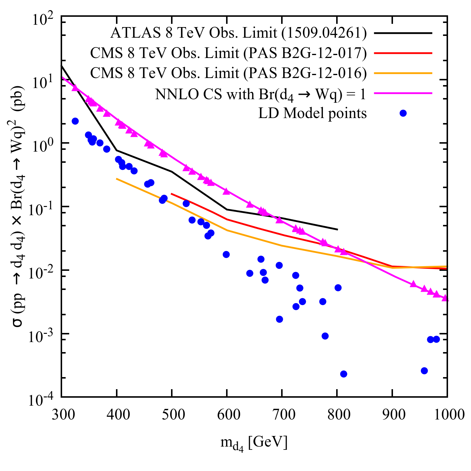
(a)

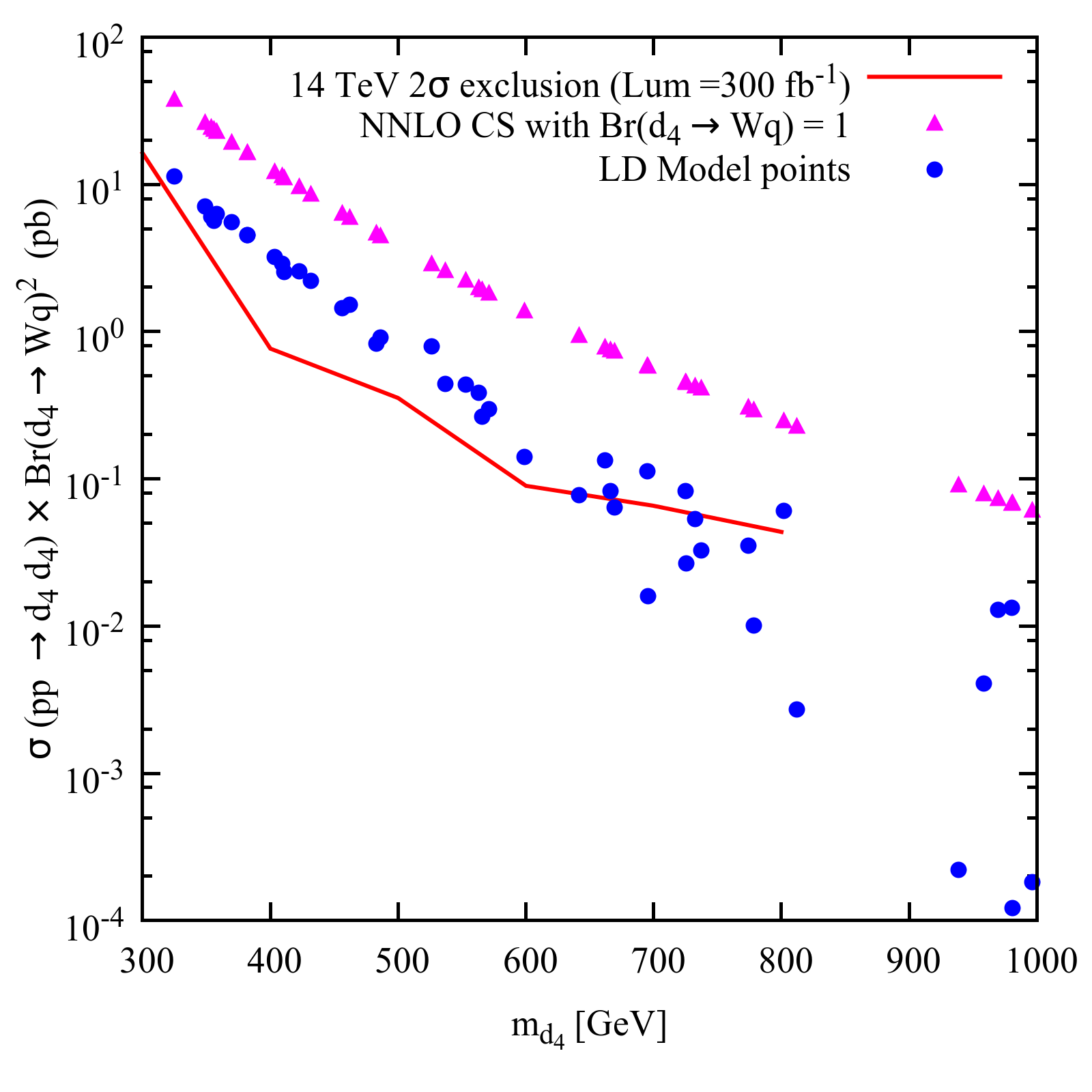
(b)

Figure 12: (a) A survey of collider constraints for the LD model in the plane ($d_{4}$, $\sigma\times\textrm{BR}(d_{4}\rightarrow W^{\pm}q)^{2}$). Points are excluded above the solid yellow line. (b) Solid red line gives our projected exclusion bound at 14$\,\mathrm{TeV}$, 300$\,\text{fb}^{-1}$.

In Fig. 12(b), we present the future projection limit for the 14$\,\mathrm{TeV}$ LHC with luminosity 300$\,\text{fb}^{-1}$. To obtain an approximate future $2\sigma$ exclusion projection, we have used the ATLAS 8$\,\mathrm{TeV}$ resultsAad:2015tba with few simplifying assumptions. We consider that the background events at 14$\,\mathrm{TeV}$ will be increased by a factor 2 compared to the 8$\,\mathrm{TeV}$ data for the same luminosity. From the ATLAS analysisAad:2015tba , we have evaluated the signal cut efficiencies for ${d_{4}}$ mass range 300 to 800$\,\mathrm{GeV}$, and we assume here that these efficiencies remain the same for the 14$\,\mathrm{TeV}$ search. We assume a background systematic uncertainty $\delta B$ of about 30% and, in the approximation of normally distributed statistics, we find the exclusion bound by applying the condition

$$\frac{S}{\sqrt{B+(B\cdot\delta B)^{2}}}>2\,,$$ (66)

where $B$ is the new number of background events and $S$ is the calculated signal.

We calculate the $d_{4}$ pair production cross section using MadGraph5 at 14$\,\mathrm{TeV}$ (multiplied with a k-factor of 1.35) and present the quantity $\sigma\times Br(d_{4}\rightarrow W^{\pm}q)^{2}$ in Fig. 12(b). It appears that VL quark masses can be excluded up to around 700$\,\mathrm{GeV}$ with 14$\,\mathrm{TeV}$ LHC data and luminosity 300$\,\text{fb}^{-1}$, even with $\textrm{BR}(d_{4}\rightarrow W^{\pm}q)\approx 0.4-0.5$.

References

- (1) CMS Collaboration, Search for direct top squark pair production in the single lepton final state at , Tech. Rep. CMS-PAS-SUS-16-028, CERN, Geneva, 2016.
- (2) CMS Collaboration, Search for supersymmetry in events with jets and missing transverse momentum in proton-proton collisions at 13 TeV, Tech. Rep. CMS-PAS-SUS-16-014, CERN, Geneva, 2016.
- (3) CMS Collaboration, Search for new physics in the all-hadronic final state with the MT2 variable, Tech. Rep. CMS-PAS-SUS-16-015, CERN, Geneva, 2016.
- (4) CMS Collaboration, An inclusive search for new phenomena in final states with one or more jets and missing transverse momentum at 13 TeV with the AlphaT variable, Tech. Rep. CMS-PAS-SUS-16-016, CERN, Geneva, 2016.
- (5) ATLAS Collaboration, Further searches for squarks and gluinos in final states with jets and missing transverse momentum at =13 TeV with the ATLAS detector, Tech. Rep. ATLAS-CONF-2016-078, CERN, Geneva, Aug, 2016.
- (6) ATLAS Collaboration, Search for top squarks in final states with one isolated lepton, jets, and missing transverse momentum in = 13 TeV pp collisions with the ATLAS detector, Tech. Rep. ATLAS-CONF-2016-050, CERN, Geneva, Aug, 2016.
- (7) ATLAS Collaboration, Search for squarks and gluinos in events with an isolated lepton, jets and missing transverse momentum at = 13 TeV with the ATLAS detector, Tech. Rep. ATLAS-CONF-2016-054, CERN, Geneva, Aug, 2016.
- (8) ATLAS Collaboration, Search for pair production of gluinos decaying via top or bottom squarks in events with -jets and large missing transverse momentum in collisions at TeV with the ATLAS detector, Tech. Rep. ATLAS-CONF-2016-052, CERN, Geneva, Aug, 2016.
- (9) K. Kowalska, Phenomenological MSSM in light of new 13 TeV LHC data, Eur. Phys. J. C76 (2016), no. 12 684, [arXiv:1608.02489].
- (10) L. Roszkowski, E. M. Sessolo, and A. J. Williams, What next for the CMSSM and the NUHM: Improved prospects for superpartner and dark matter detection, JHEP 08 (2014) 067, [arXiv:1405.4289].
- (11) Muon g-2 Collaboration, G. W. Bennett et al., Final Report of the Muon E821 Anomalous Magnetic Moment Measurement at BNL, Phys. Rev. D73 (2006) 072003, [hep-ex/0602035].
- (12) J. P. Miller, E. de Rafael, and B. L. Roberts, Muon (g-2): Experiment and theory, Rept. Prog. Phys. 70 (2007) 795, [hep-ph/0703049].
- (13) Muon g-2 Collaboration, J. Grange et al., Muon (g-2) Technical Design Report, arXiv:1501.06858.
- (14) Muon g-2 Collaboration, A. Chapelain, The Muon g-2 experiment at Fermilab, EPJ Web Conf. 137 (2017) 08001, [arXiv:1701.02807].
- (15) M. Endo, K. Hamaguchi, S. Iwamoto, and T. Yoshinaga, Muon g-2 vs LHC in Supersymmetric Models, JHEP 01 (2014) 123, [arXiv:1303.4256].
- (16) A. Fowlie, K. Kowalska, L. Roszkowski, E. M. Sessolo, and Y.-L. S. Tsai, Dark matter and collider signatures of the MSSM, Phys. Rev. D88 (2013) 055012, [arXiv:1306.1567].
- (17) M. Chakraborti, U. Chattopadhyay, A. Choudhury, A. Datta, and S. Poddar, The Electroweak Sector of the pMSSM in the Light of LHC - 8 TeV and Other Data, JHEP 07 (2014) 019, [arXiv:1404.4841].
- (18) S. P. Das, M. Guchait, and D. P. Roy, Testing SUSY models for the muon g-2 anomaly via chargino-neutralino pair production at the LHC, Phys. Rev. D90 (2014), no. 5 055011, [arXiv:1406.6925].
- (19) M. Lindner, M. Platscher, and F. S. Queiroz, A Call for New Physics : The Muon Anomalous Magnetic Moment and Lepton Flavor Violation, arXiv:1610.06587.
- (20) A. Fowlie, M. Kazana, K. Kowalska, S. Munir, L. Roszkowski, E. M. Sessolo, S. Trojanowski, and Y.-L. S. Tsai, The CMSSM Favoring New Territories: The Impact of New LHC Limits and a 125 GeV Higgs, Phys. Rev. D86 (2012) 075010, [arXiv:1206.0264].
- (21) S. Mohanty, S. Rao, and D. P. Roy, Reconciling the muon and dark matter relic density with the LHC results in nonuniversal gaugino mass models, JHEP 09 (2013) 027, [arXiv:1303.5830].
- (22) S. Akula and P. Nath, Gluino-driven radiative breaking, Higgs boson mass, muon g-2, and the Higgs diphoton decay in supergravity unification, Phys. Rev. D87 (2013), no. 11 115022, [arXiv:1304.5526].
- (23) J. Chakrabortty, S. Mohanty, and S. Rao, Non-universal gaugino mass GUT models in the light of dark matter and LHC constraints, JHEP 02 (2014) 074, [arXiv:1310.3620].
- (24) K. Kowalska, L. Roszkowski, E. M. Sessolo, and A. J. Williams, GUT-inspired SUSY and the muon anomaly: prospects for LHC 14 TeV, JHEP 06 (2015) 020, [arXiv:1503.08219].
- (25) J. Chakrabortty, A. Choudhury, and S. Mondal, Non-universal Gaugino mass models under the lamppost of muon (g-2), JHEP 07 (2015) 038, [arXiv:1503.08703].
- (26) A. S. Belyaev, J. E. Camargo-Molina, S. F. King, D. J. Miller, A. P. Morais, and P. B. Schaefers, A to Z of the Muon Anomalous Magnetic Moment in the MSSM with Pati-Salam at the GUT scale, JHEP 06 (2016) 142, [arXiv:1605.02072].
- (27) N. Okada and H. M. Tran, 125 GeV Higgs boson mass and muon in 5D MSSM, Phys. Rev. D94 (2016), no. 7 075016, [arXiv:1606.05329].
- (28) T. Fukuyama, N. Okada, and H. M. Tran, Sparticle spectroscopy of the minimal SO(10) model, Phys. Lett. B767 (2017) 295–302, [arXiv:1611.08341].
- (29) M. Endo, K. Hamaguchi, S. Iwamoto, and N. Yokozaki, Higgs mass, muon , and LHC prospects in gauge mediation models with vector-like matters, Phys. Rev. D85 (2012) 095012, [arXiv:1112.5653].
- (30) M. Endo, K. Hamaguchi, S. Iwamoto, and N. Yokozaki, Higgs Mass and Muon Anomalous Magnetic Moment in Supersymmetric Models with Vector-Like Matters, Phys. Rev. D84 (2011) 075017, [arXiv:1108.3071].
- (31) R. Dermisek and A. Raval, Explanation of the Muon g-2 Anomaly with Vectorlike Leptons and its Implications for Higgs Decays, Phys. Rev. D88 (2013) 013017, [arXiv:1305.3522].
- (32) R. Dermisek, A. Raval, and S. Shin, Effects of vectorlike leptons on and the connection to the muon g-2 anomaly, Phys. Rev. D90 (2014), no. 3 034023, [arXiv:1406.7018].
- (33) I. Gogoladze, Q. Shafi, and C. S. Un, Reconciling the muon g-2, a 125 GeV Higgs boson, and dark matter in gauge mediation models, Phys. Rev. D92 (2015), no. 11 115014, [arXiv:1509.07906].
- (34) A. Aboubrahim, T. Ibrahim, and P. Nath, Leptonic moments, CP phases and the Higgs boson mass constraint, Phys. Rev. D94 (2016), no. 1 015032, [arXiv:1606.08336].
- (35) M. Nishida and K. Yoshioka, Higgs Boson Mass and Muon g-2 with Strongly Coupled Vector-like Generations, Phys. Rev. D94 (2016), no. 9 095022, [arXiv:1605.06675].
- (36) T. Higaki, M. Nishida, and N. Takeda, Flavor Structure, Higgs boson mass and Dark Matter in Supersymmetric Model with Vector-like Generations, arXiv:1611.04322.
- (37) E. Megias, M. Quiros, and L. Salas, from Vector-Like Leptons in Warped Space, JHEP 05 (2017) 016, [arXiv:1701.05072].
- (38) S. P. Martin, Extra vector-like matter and the lightest Higgs scalar boson mass in low-energy supersymmetry, Phys. Rev. D81 (2010) 035004, [arXiv:0910.2732].
- (39) P. W. Graham, A. Ismail, S. Rajendran, and P. Saraswat, A Little Solution to the Little Hierarchy Problem: A Vector-like Generation, Phys. Rev. D81 (2010) 055016, [arXiv:0910.3020].
- (40) C. Faroughy and K. Grizzard, Raising the Higgs mass in supersymmetry with t-t′ mixing, Phys. Rev. D90 (2014), no. 3 035024, [arXiv:1405.4116].
- (41) Z. Lalak, M. Lewicki, and J. D. Wells, Higgs boson mass and high-luminosity LHC probes of supersymmetry with vectorlike top quark, Phys. Rev. D91 (2015), no. 9 095022, [arXiv:1502.05702].
- (42) K. Nickel and F. Staub, Precise determination of the Higgs mass in supersymmetric models with vectorlike tops and the impact on naturalness in minimal GMSB, JHEP 07 (2015) 139, [arXiv:1505.06077].
- (43) R. Barbieri, D. Buttazzo, L. J. Hall, and D. Marzocca, Higgs mass and unified gauge coupling in the NMSSM with Vector Matter, JHEP 07 (2016) 067, [arXiv:1603.00718].
- (44) A. Angelescu, A. Djouadi, and G. Moreau, Vector-like top/bottom quark partners and Higgs physics at the LHC, Eur. Phys. J. C76 (2016), no. 2 99, [arXiv:1510.07527].
- (45) Measurements of the Higgs boson production and decay rates and constraints on its couplings from a combined ATLAS and CMS analysis of the LHC pp collision data at = 7 and 8 TeV, Tech. Rep. ATLAS-CONF-2015-044, CERN, Geneva, Sep, 2015.
- (46) R. Dermisek, Loop suppressed electroweak symmetry breaking and naturally heavy superpartners, Phys. Rev. D95 (2017), no. 1 015002, [arXiv:1606.09031].
- (47) T. Ibrahim, A. Itani, and P. Nath, decay in an MSSM extension, Phys. Rev. D92 (2015), no. 1 015003, [arXiv:1503.01078].
- (48) A. Aboubrahim, T. Ibrahim, and P. Nath, Neutron electric dipole moment and probe of PeV scale physics, Phys. Rev. D91 (2015), no. 9 095017, [arXiv:1503.06850].
- (49) A. Aboubrahim, T. Ibrahim, P. Nath, and A. Zorik, Chromoelectric Dipole Moments of Quarks in MSSM Extensions, Phys. Rev. D92 (2015), no. 3 035013, [arXiv:1507.02668].
- (50) S. Fathy, T. Ibrahim, A. Itani, and P. Nath, Flavor violating leptonic decays of the Higgs boson, Phys. Rev. D94 (2016), no. 11 115029, [arXiv:1608.05998].
- (51) C. D. Froggatt and H. B. Nielsen, Hierarchy of Quark Masses, Cabibbo Angles and CP Violation, Nucl. Phys. B147 (1979) 277–298.
- (52) A. E. Nelson and D. Wright, Horizontal, anomalous U(1) symmetry for the more minimal supersymmetric standard model, Phys. Rev. D56 (1997) 1598–1604, [hep-ph/9702359].
- (53) W. Porod, SPheno, a program for calculating supersymmetric spectra, SUSY particle decays and SUSY particle production at e+ e- colliders, Comput.Phys.Commun. 153 (2003) 275–315.
- (54) W. Porod and F. Staub, SPheno 3.1: Extensions including flavour, CP-phases and models beyond the MSSM, Comput.Phys.Commun. 183 (2012) 2458–2469.
- (55) F. Staub, SARAH, arXiv:0806.0538.
- (56) F. Staub, Automatic Calculation of supersymmetric Renormalization Group Equations and Self Energies, Comput.Phys.Commun. 182 (2011) 808–833.
- (57) F. Staub, From Superpotential to Model Files for FeynArts and CalcHep/CompHep, Comput.Phys.Commun. 181 (2010) 1077–1086.
- (58) F. Staub, SARAH 3.2: Dirac Gauginos, UFO output, and more, Comput.Phys.Commun. 184 (2013) pp. 1792–1809.
- (59) F. Staub, SARAH 4: A tool for (not only SUSY) model builders, Comput.Phys.Commun. 185 (2014) 1773–1790.
- (60) F. Staub et al., Precision tools and models to narrow in on the 750 GeV diphoton resonance, Eur. Phys. J. C76 (2016), no. 9 516, [arXiv:1602.05581].
- (61) J. R. Ellis, K. Enqvist, D. V. Nanopoulos, and F. Zwirner, Observables in Low-Energy Superstring Models, Mod. Phys. Lett. A1 (1986) 57.
- (62) R. Barbieri and G. F. Giudice, Upper Bounds on Supersymmetric Particle Masses, Nucl. Phys. B306 (1988) 63–76.
- (63) G. G. Ross, K. Schmidt-Hoberg, and F. Staub, Revisiting fine-tuning in the MSSM, JHEP 03 (2017) 021, [arXiv:1701.03480].
- (64) Particle Data Group Collaboration, C. Patrignani et al., Review of Particle Physics, Chin. Phys. C40 (2016), no. 10 100001.
- (65) R. Dermisek, E. Lunghi, and S. Shin, Two Higgs doublet model with vectorlike leptons and contributions to and , JHEP 02 (2016) 119, [arXiv:1509.04292].
- (66) K. Hagiwara, R. Liao, A. D. Martin, D. Nomura, and T. Teubner, and re-evaluated using new precise data, J. Phys. G38 (2011) 085003, [arXiv:1105.3149].
- (67) M. Davier, Update of the Hadronic Vacuum Polarisation Contribution to the muon g-2, in 14th International Workshop on Tau Lepton Physics (TAU 2016) Beijing, China, September 19-23, 2016, 2016. arXiv:1612.02743.
- (68) M. Davier, A. Hoecker, B. Malaescu, and Z. Zhang, Reevaluation of the Hadronic Contributions to the Muon g-2 and to alpha(MZ), Eur. Phys. J. C71 (2011) 1515, [arXiv:1010.4180]. [Erratum: Eur. Phys. J.C72,1874(2012)].
- (69) P. Bechtle et al., Constrained Supersymmetry after two years of LHC data: a global view with Fittino, JHEP 06 (2012) 098, [arXiv:1204.4199].
- (70) O. Buchmueller et al., The CMSSM and NUHM1 after LHC Run 1, Eur. Phys. J. C74 (2014), no. 6 2922, [arXiv:1312.5250].
- (71) T. Moroi, The Muon anomalous magnetic dipole moment in the minimal supersymmetric standard model, Phys. Rev. D53 (1996) 6565–6575, [hep-ph/9512396]. [Erratum: Phys. Rev.D56,4424(1997)].
- (72) S. P. Martin and J. D. Wells, Muon anomalous magnetic dipole moment in supersymmetric theories, Phys. Rev. D64 (2001) 035003, [hep-ph/0103067].
- (73) F. Feroz, M. P. Hobson, and M. Bridges, MultiNest: an efficient and robust Bayesian inference tool for cosmology and particle physics, Mon. Not. Roy. Astron. Soc. 398 (2009) 1601–1614, [arXiv:0809.3437].
- (74) W. Porod, F. Staub, and A. Vicente, A Flavor Kit for BSM models, Eur. Phys. J. C74 (2014), no. 8 2992, [arXiv:1405.1434].
- (75) G. Belanger, F. Boudjema, A. Pukhov, and A. Semenov, micrOMEGAs3: A program for calculating dark matter observables, Comput. Phys. Commun. 185 (2014) 960–985, [arXiv:1305.0237].
- (76) P. Bechtle, S. Heinemeyer, O. Stål, T. Stefaniak, and G. Weiglein, : Confronting arbitrary Higgs sectors with measurements at the Tevatron and the LHC, Eur. Phys. J. C74 (2014), no. 2 2711, [arXiv:1305.1933].
- (77) P. Bechtle, O. Brein, S. Heinemeyer, G. Weiglein, and K. E. Williams, HiggsBounds: Confronting Arbitrary Higgs Sectors with Exclusion Bounds from LEP and the Tevatron, Comput. Phys. Commun. 181 (2010) 138–167, [arXiv:0811.4169].
- (78) P. Bechtle, O. Brein, S. Heinemeyer, G. Weiglein, and K. E. Williams, HiggsBounds 2.0.0: Confronting Neutral and Charged Higgs Sector Predictions with Exclusion Bounds from LEP and the Tevatron, Comput. Phys. Commun. 182 (2011) 2605–2631, [arXiv:1102.1898].
- (79) P. Bechtle, O. Brein, S. Heinemeyer, O. Stål, T. Stefaniak, G. Weiglein, and K. E. Williams, : Improved Tests of Extended Higgs Sectors against Exclusion Bounds from LEP, the Tevatron and the LHC, Eur. Phys. J. C74 (2014), no. 3 2693, [arXiv:1311.0055].
- (80) LUX Collaboration, D. S. Akerib et al., Results from a search for dark matter in the complete LUX exposure, Phys. Rev. Lett. 118 (2017), no. 2 021303, [arXiv:1608.07648].
- (81) Planck Collaboration, P. A. R. Ade et al., Planck 2015 results. XIII. Cosmological parameters, Astron. Astrophys. 594 (2016) A13, [arXiv:1502.01589].
- (82) Y. Amhis et al., Averages of -hadron, -hadron, and -lepton properties as of summer 2016, arXiv:1612.07233.
- (83) Belle Collaboration, I. Adachi et al., Evidence for with a Hadronic Tagging Method Using the Full Data Sample of Belle, Phys. Rev. Lett. 110 (2013), no. 13 131801, [arXiv:1208.4678].
- (84) LHCb Collaboration, R. Aaij et al., Measurement of the branching fraction and search for decays at the LHCb experiment, Phys. Rev. Lett. 111 (2013) 101805, [arXiv:1307.5024].
- (85) CMS Collaboration, S. Chatrchyan et al., Measurement of the B(s) to mu+ mu- branching fraction and search for B0 to mu+ mu- with the CMS Experiment, Phys. Rev. Lett. 111 (2013) 101804, [arXiv:1307.5025].
- (86) BaBar Collaboration, B. Aubert et al., Searches for Lepton Flavor Violation in the Decays and , Phys. Rev. Lett. 104 (2010) 021802, [arXiv:0908.2381].
- (87) ATLAS Collaboration, Search for supersymmetry with two and three leptons and missing transverse momentum in the final state at TeV with the ATLAS detector, Tech. Rep. ATLAS-CONF-2016-096, CERN, Geneva, Sep, 2016.
- (88) CMS Collaboration, C. Collaboration, Search for electroweak SUSY production in multilepton final states in pp collisions at sqrt(s)=13 TeV with 12.9/fb, .
- (89) W. Altmannshofer and D. M. Straub, New physics in transitions after LHC run 1, Eur. Phys. J. C75 (2015), no. 8 382, [arXiv:1411.3161].
- (90) S. Descotes-Genon, L. Hofer, J. Matias, and J. Virto, Global analysis of anomalies, JHEP 06 (2016) 092, [arXiv:1510.04239].
- (91) T. Moroi, R. Sato, and T. T. Yanagida, Extra Matters Decree the Relatively Heavy Higgs of Mass about 125 GeV in the Supersymmetric Model, Phys. Lett. B709 (2012) 218–221, [arXiv:1112.3142].
- (92) M. Abdullah and J. L. Feng, Reviving bino dark matter with vectorlike fourth generation particles, Phys. Rev. D93 (2016), no. 1 015006, [arXiv:1510.06089].
- (93) M. Abdullah, J. L. Feng, S. Iwamoto, and B. Lillard, Heavy bino dark matter and collider signals in the MSSM with vectorlike fourth-generation particles, Phys. Rev. D94 (2016), no. 9 095018, [arXiv:1608.00283].
- (94) XENON Collaboration, E. Aprile et al., Physics reach of the XENON1T dark matter experiment, JCAP 1604 (2016), no. 04 027, [arXiv:1512.07501].
- (95) L3 Collaboration, P. Achard et al., Search for heavy neutral and charged leptons in annihilation at LEP, Phys. Lett. B517 (2001) 75–85, [hep-ex/0107015].
- (96) N. Kumar and S. P. Martin, Vectorlike leptons at the Large Hadron Collider, Phys. Rev. D92 (2015), no. 11 115018, [arXiv:1510.03456].
- (97) R. Dermisek, J. P. Hall, E. Lunghi, and S. Shin, Limits on Vectorlike Leptons from Searches for Anomalous Production of Multi-Lepton Events, JHEP 12 (2014) 013, [arXiv:1408.3123].
- (98) ATLAS Collaboration, G. Aad et al., Search for heavy lepton resonances decaying to a boson and a lepton in collisions at TeV with the ATLAS detector, JHEP 09 (2015) 108, [arXiv:1506.01291].
- (99) ATLAS Collaboration, G. Aad et al., Search for pair production of a new heavy quark that decays into a boson and a light quark in collisions at TeV with the ATLAS detector, Phys. Rev. D92 (2015), no. 11 112007, [arXiv:1509.04261].
- (100) CMS Collaboration, C. Collaboration, Search for exotic light-flavor quark partners in pp collisions at , .
- (101) CMS Collaboration, C. Collaboration, Search for vector-like quarks in final states with a single lepton and jets in pp collisions at sqrt s = 8 TeV, .
- (102) J. Alwall, R. Frederix, S. Frixione, V. Hirschi, F. Maltoni, O. Mattelaer, H. S. Shao, T. Stelzer, P. Torrielli, and M. Zaro, The automated computation of tree-level and next-to-leading order differential cross sections, and their matching to parton shower simulations, JHEP 07 (2014) 079, [arXiv:1405.0301].