Omnidirectional spin Hall effect in a Weyl spin-orbit coupled atomic gas

Abstract

We show that in the presence of a three-dimensional (Weyl) spin-orbit coupling, a transverse spin current is generated in response to either a constant spin-independent force or a time-dependent Zeeman field in an arbitrary direction. This effect is the non-Abelian counterpart of the universal intrinsic spin Hall effect characteristic to the two-dimensional Rashba spin-orbit coupling. We quantify the strength of such an omnidirectional spin Hall effect by calculating the corresponding conductivity for fermions and non-condensed bosons. The absence of any kind of disorder in ultracold-atom systems makes the observation of this effect viable.

I Introduction

Gauge theories and related geometrical concepts play a prominent role in the description of physics at a wide range of length scales covering all fundamental interactions Frankel (2004). On the other hand, when it comes to effective models, many quantum-mechanical systems with adiabatically varying parameters are naturally described in terms of Abelian gauge theories Berry (1984); Shapere and Wilczek (1989); Bohm et al. (2003). This geometric approach based on the Berry phase has paved the way to a multitude of both theoretical and experimental developments covering molecular Shapere and Wilczek (1989); Bohm et al. (2003); Mead (1992), solid-state Loss et al. (1990); Lévy et al. (1990); Chandrasekhar et al. (1991); Mailly et al. (1993); Neubauer et al. (2009); Li et al. (2013a); Hasan and Kane (2010), photonic Bliokh et al. (2008); Hafezi et al. (2011); Kitagawa et al. (2013); Rechtsman et al. (2013); Mittal et al. (2014); Tzuang et al. (2014); Dubček et al. (2015); Skirlo et al. (2015); Ozawa et al. (2016), mechanical Süsstrunk and Huber (2015); Salerno et al. (2016) and electric Ningyuan et al. (2015); Albert et al. (2015) systems. Although the corresponding non-Abelian gauge structure in the presence of degenerate quantum states has been noticed promptly after the discovery of the Berry phase Wilczek and Zee (1984), a set of experimentally observed signatures of the non-Abelian geometrical phases remains limited Zee (1988); Zwanziger et al. (1990).

Ultracold-atom experiments have been recently gaining tools uniquely suited to address this elusive non-Abelian gauge structure using the internal states of the atom Lin et al. (2009a, b); Aidelsburger et al. (2011); Struck et al. (2012); Aidelsburger et al. (2013); Miyake et al. (2013); Kennedy et al. (2013); Armaitis et al. (2013); Choi et al. (2013); Jotzu et al. (2014); Aidelsburger et al. (2014); Atala et al. (2014); Fläschner et al. (2016); Li et al. (2016); Stuhl et al. (2015); Mancini et al. (2015). In particular, engineering various species of spin-orbit coupling Dudarev et al. (2004); Ruseckas et al. (2005); Osterloh et al. (2005); Juzeliūnas et al. (2008); Stanescu et al. (2007); Vaishnav and Clark (2008); Liu et al. (2009); Zhang (2010); Campbell et al. (2011); Dalibard et al. (2011); Anderson et al. (2012); Xu et al. (2013); Anderson et al. (2013); Zhou et al. (2013); Anderson and Clark (2013); Li et al. (2013b); Galitski and Spielman (2013); Goldman et al. (2014); Zhai (2015) in ultracold-atom systems has seen rapid advances lately Lin et al. (2011); Zhang et al. (2012); Wang et al. (2012); Cheuk et al. (2012); Williams et al. (2012); LeBlanc et al. (2013); Qu et al. (2013); Fu et al. (2014); Huang et al. (2016); Meng et al. (2016); Wu et al. (2016), allowing experimental demonstration of, e.g., the phase diagram of spin-orbit coupled (SOC) bosons Ji et al. (2014) and the spin Hall effect Beeler et al. (2013). However, despite the existence of this novel toolbox, there is a lack of concrete proposals to unambiguously demonstrate the non-Abelian gauge structure.

The spin Hall effect (SHE), in which density currents generate transverse spin currents has already played a prominent role in condensed-matter physics and has provided an impetus to the field of spintronics Sinova et al. (2015). The SHE has been detected experimentally in a wide variety of solid-state materials, which usualy possess a planar SOC of the Rashba-Dresselhaus type. In these solid-state experiments, the SOC plane corresponds to the two-dimensional (2D) geometry of the sample. Therefore, both the perturbation of the system (applied voltage) and the resulting spin current are confined to that plane. On the other hand, the spin current is polarized in the direction perpendicular to the SOC plane. This spin Hall effect is induced by a spin-dependent Berry magnetic field (Berry curvature) perpendicular to the plane. Such a magnetic field is proportional to a single Pauli matrix $\sigma_{z}$ and hence is Abelian, as it will be discussed in more details in the next Section.

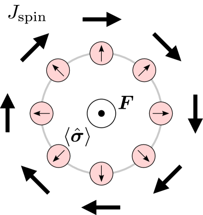
Figure 1: In a Weyl spin-orbit coupled system, a spin-independent force pointing in an arbitrary direction drives a spin current in the plane perpendicular to the force. Here we show this situation in the momentum space. Particles with spins $\langle\hat{\boldsymbol{\sigma}}\rangle$ respond to the force $\boldsymbol{F}$ by contributing to the spin current $J_{\text{spin}}$ which runs perpendicular to the force and carries the spin orthogonal to both the current and the force, see Eq. (28). The independence of this phenomenon from the driving direction unambiguously demonstrates the non-Abelian nature of the underlying dynamics.

In the present article we put forward a three-dimensional (3D) version of the SHE based on the novel possibility to engineer a nonplanar spin-orbit coupling of the Weyl type for ultracold atoms Anderson et al. (2012, 2013); Zhou et al. (2013); Anderson and Clark (2013); Tokatly and Sherman (2016). In the proposed setup, the atoms are affected by a 3D Berry magnetic field which is non-Abelian and induces a spin-dependent Lorentz-type force for all directions of atomic motion. Perturbing the system along an arbitrary axis produces a spin current perpendicular to the perturbation (Fig. 1). Such a response is in a stark contrast to the Abelian case, where the magnetic field unavoidably has a single well-defined direction, and the (spin) Hall effect occurs in the plane perpendicular to it. We will refer to the present effect based on the 3D SOC as an omnidirectional spin Hall effect which is the non-Abelian counterpart of the universal intrinsic spin Hall effect characteristic to the two-dimensional Rashba SOC Sinova et al. (2004).

In certain lattice systems Burkov and Balents (2011); Ando (2013); Borisenko et al. (2014); Liu et al. (2014); Xu et al. (2015); Lu et al. (2015); Soluyanov et al. (2015); Lv et al. (2015); Dubček et al. (2015), pairs of Weyl points of opposite topological charges arise governing the topological properties Burkov and Balents (2011); Wan et al. (2011) or interactions between particles Gürsoy et al. (2013) in the so-called Weyl semimetal regime. Since the Weyl points have opposite topological charges, they respond to driving in an opposite way, and the induced spin-currents cancel. Here we consider the SOC of the Weyl type (also known as the Weyl-Rashba SOC) produced by manipulating atomic internal states Anderson et al. (2012, 2013); Zhou et al. (2013); Anderson and Clark (2013) rather than using a lattice, so only a single Weyl point arises. This is an important feature for generating a nonzero spin current in response to a spin-independent force.

In the present study we do not include the effects due to impurities. The impurities play a crucial role in the spin Hall effect physics for electrons in solids to the extent of preventing the universal intrinsic spin Hall effect Dimitrova (2005); Khaetskii (2006); Sinova et al. (2015). However, ultracold-atoms are free from impurity scattering, both magnetic and nonmagnetic, so the spin-Hall effect is not suppressed in these systems.

Furthermore, interactions between the ultracold-atoms are typically weak Leggett (2001), and they can be further minimized by utilizing the Feshbach resonances Chin et al. (2010). We therefore leave the detailed study of interaction effects Guan and Blume (2017) for future work.

The paper is organized as follows. In Section  II we define the atomic Hamiltonian with the Weyl SOC included, and write down the equations of motion for the spin and center-of-mass degrees of freedom. Section III explores spin currents in this system, and presents the possibility to generate a transverse spin current for any direction of the applied perturbation. The concluding Section IV summarizes the findings and outlines possible future directions. In Appendix, we discuss in more detail the definition of the spin current used in the main text, and consider a relationship between spin (Stern-Gerlach) projection measurement and and the spin Hall current.

II Theoretical framework and non-Abelian dynamics

II.1 Hamiltonian

Let us consider an ensemble of atoms subjected to a Weyl (3D) SOC of a strength $\chi$. Individual atoms are described by the Hamiltonian

$$\hat{H}=(\boldsymbol{p}-\hat{\mathbfcal A})^{2}/2m+U,\quad\hat{\mathbfcal A}=\chi\hat{\boldsymbol{\sigma}}+\beta\boldsymbol{e}_{\beta}\,,$$ (1)

where the Weyl SOC is due to the vector of Pauli matrices $\hat{\boldsymbol{\sigma}}=\hat{\sigma}_{x}\boldsymbol{e}_{x}+\hat{\sigma}_{y}\boldsymbol{e}_{y}+\hat{\sigma}_{z}\boldsymbol{e}_{z}$ entering the vector potential $\hat{\mathbfcal A}$. An extra term $\beta\boldsymbol{e}_{\beta}$ provides a spatially uniform spin-independent driving force $\dot{\beta}\boldsymbol{e}_{\beta}$ perturbing the atoms along a unit vector $e_{\beta}$, the dot denoting a time derivative. Here $U$ is a spin-independent trapping potential. We suppress the identity matrix in the spin space and set $\hbar=1$ at the outset. In Eq. (1) the bold font specifies a spatial vector, whereas the hat indicates an operator acting on the atomic internal (pseudo-) spin states. Moreover, $\boldsymbol{p}$ is a momentum operator and $m$ is an atomic mass. Although for concreteness we consider (pseudo-) spin 1/2 atoms, generalization to a higher-spin system is straightforward and does not change the qualitative picture.

The Hamiltonian in Eq. (1) yields two dispersion branches for an unperturbed atom ($\beta=0$) affected by the Weyl SOC:

$$\varepsilon_{p\pm}=\left(p^{2}\pm 2{\chi p}+\chi^{2}\right)/2m=\left(p\pm\chi\right)^{2}/2m\,,$$ (2)

where the lower (upper) sign corresponds to the lower (upper) dispersion branch in which the spin points along (opposite to) the momentum $\boldsymbol{p}$. In writing Eq. (2) we have added a constant to place the minimum of the lower dispersion branch at the zero energy: $\varepsilon_{\chi-}=0$.

II.2 Equations of motion

Defining a velocity operator for an atom via the Heisenberg equation

$$\hat{\boldsymbol{v}}=-i[\boldsymbol{r},\hat{H}]=(\boldsymbol{p}-\hat{\mathbfcal A})/m\,,$$ (3)

one can rewrite the Hamiltonian in a concise manner: $\hat{H}=m\hat{\boldsymbol{v}}^{2}/2+U$, where $\boldsymbol{r}$ is a position operator. The velocity operator $\hat{\boldsymbol{v}}$ contains a vector potential $\hat{\mathbfcal A}$ which is an operator acting in the spin space. Hence $\hat{\boldsymbol{v}}$ obeys the following non-trivial Heisenberg equation of motion Goldman et al. (2014)

$$m\dot{\hat{\boldsymbol{v}}}=(\hat{\boldsymbol{v}}\times\hat{\mathbfcal B}-\hat{\mathbfcal B}\times\hat{\boldsymbol{v}})/2-\boldsymbol{\nabla}U+\hat{\mathbfcal E}\,,$$ (4)

where

$$\hat{\mathbfcal E}=-\partial_{t}\hat{\mathbfcal A}=-\dot{\beta}\boldsymbol{e}_{\beta}$$ (5)

is the strength of the perturbing Berry electric field, and

$$\hat{\mathbfcal B}=-i\hat{\mathbfcal A}\times\hat{\mathbfcal A}=2\chi^{2}\hat{\boldsymbol{\sigma}}$$ (6)

is the strength of the Berry magnetic field.

The latter magnetic field $\hat{\mathbfcal B}$ is proportional to the spin operator $\hat{\boldsymbol{\sigma}}$. Hence, it has non-commuting Cartesian components, showing a non-Abelian character of $\hat{\mathbfcal B}$. This is in contrast to the usual planar Rashba-type spin-orbit coupling for which $\hat{\mathbfcal A}\propto\hat{\sigma}_{x}\boldsymbol{e}_{x}+\hat{\sigma}_{y}\boldsymbol{e}_{y}$, so the Berry magnetic field strength $\hat{\mathbfcal B}\propto\hat{\sigma}_{z}\boldsymbol{e}_{z}$ contains commuting Cartesian components, and is thus Abelian. Note that the components of the spatially uniform Berry magnetic field (6) can be written in terms of the field strength $\hat{\mathcal{F}}_{ab}=-i[\hat{\mathcal{A}}_{a},\hat{\mathcal{A}}_{b}]$ Wilczek and Zee (1984), also known as the Yang-Mills curvature Fujita et al. (2011): $\hat{\mathcal{B}}_{a}=\sum_{b,c}\epsilon_{abc}\hat{\mathcal{F}}_{bc}/2$. Genuine non-Abelian dynamics occurs only in systems where $[\hat{\mathcal{F}}_{ab},\hat{\mathcal{F}}_{cd}]\neq 0$, as discussed in detail in Ref. Goldman et al. (2014). Indeed, our system falls into the non-Abelian-dynamics class, as here $\hat{\mathcal{F}}_{ab}=2\chi^{2}\sum_{c}\epsilon_{abc}\hat{\sigma}_{c}$.

The spin-dependent part of the Hamiltonian (1) can be represented as $-\boldsymbol{M}\cdot\hat{\boldsymbol{\sigma}}$, where we have introduced an effective magnetic field

$$\boldsymbol{M}=\chi\boldsymbol{p}^{\prime}/m\,,\quad\boldsymbol{p}^{\prime}=\boldsymbol{p}-\beta\boldsymbol{e}_{\beta}\,,$$ (7)

with $\boldsymbol{p}^{\prime}$ being a momentum shifted by the spin-independent driving term $\beta\boldsymbol{e}_{\beta}$. The spin dynamics follows a Landau-Lifshitz type Landau and Lifshitz (1935) equation (LLE)

$$\dot{\hat{\boldsymbol{\sigma}}}=-i[\hat{\boldsymbol{\sigma}},\hat{H}]=2\hat{\boldsymbol{\sigma}}\times\boldsymbol{M}\,,$$ (8)

where for our dissipationless cold-atom system we have not added the Gilbert damping Gilbert (2004) term usually present when describing the magnetization dynamics in solids. One can now write down the following concise equation of motion for the velocity in terms of $\boldsymbol{M}$:

$$m\dot{\hat{\boldsymbol{v}}}=-\dot{\beta}\boldsymbol{e}_{\beta}+2\chi\boldsymbol{M}\times\hat{\boldsymbol{\sigma}}-\boldsymbol{\nabla}U\,.$$ (9)

Equations (8) and (9) describe the full atomic dynamics which involves both internal and center-of-mass degrees of freedom. From now on we consider a homogeneous system for which $U=0$. This condition is viable in a harmonic trap in the local density approximation Leggett (2001) sense, or, alternatively, in a flat trap Gaunt et al. (2013) away from the boundaries of the trap. In such a homogeneous case, the momentum $\boldsymbol{p}$ is an integral of motion: $\dot{\boldsymbol{p}}=0$. Therefore, dynamics in the spin sector completely determines the evolution of the system.

II.3 Adiabatic approach

Since the momentum $\boldsymbol{p}$ is conserved, we will henceforth work with momentum eigenstates and treat $\boldsymbol{p}$ and $\boldsymbol{M}$ as ordinary vectors rather than operators. The equation of motion for the quantum expectation value $\langle\hat{\boldsymbol{\sigma}}\rangle$ then has the same form as Eq. (8) for the spin operator $\hat{\boldsymbol{\sigma}}/2$. Hence one arrives at the following solution for the expectation value to the first order in time derivatives of $\boldsymbol{M}$ (see Refs. van der Bijl and Duine (2011); Huang (2016) for more details):

$$\langle\hat{\boldsymbol{\sigma}}\rangle_{\pm}=\pm S\left(\frac{\boldsymbol{M}}{M}+\frac{1}{2M^{3}}\boldsymbol{M}\times\dot{\boldsymbol{M}}\right)\,,$$ (10)

where the upper (lower) sign pertains to upper (lower) dispersion branch in which spin points along (opposite to) the effective magnetic field. Here

$$M\equiv|\boldsymbol{M}|=\chi|\boldsymbol{p}^{\prime}|/m\,,\quad\dot{\boldsymbol{M}}=-\chi\dot{\beta}\boldsymbol{e}_{\beta}/m\,,$$ (11)

and the normalization factor

$$S=\big{(}1+[\dot{\beta}{m}/{2\chi|\boldsymbol{p}^{\prime}|^{2}}]^{2}\big{)}^{-1/2}\simeq 1$$ (12)

ensures that $\langle\hat{\boldsymbol{\sigma}}\rangle^{2}_{\pm}=1$. The condition $S\simeq 1$ defines a range of validity of Eq. (10):

$$\dot{\beta}{m}/{2\chi|\boldsymbol{p}^{\prime}|^{2}}\ll 1.$$ (13)

In this adiabatic approach the spin expectation value is determined by the momentum-dependent effective magnetic field $\boldsymbol{M}$, as well as by the correction term containing the time-derivative $\dot{\boldsymbol{M}}$ due to the external force. In the zero-order adiabatic approximation, the spin follows the effective magnetic field: $\langle\hat{\boldsymbol{\sigma}}^{(0)}\rangle_{\pm}=\pm\boldsymbol{M}/M=\pm\boldsymbol{p}^{\prime}/p^{\prime}$. The first-order correction $\langle\hat{\boldsymbol{\sigma}}^{(1)}\rangle_{\pm}=\pm\boldsymbol{M}\times\dot{\boldsymbol{M}}/2M^{3}$ is given by

$$\langle\hat{\boldsymbol{\sigma}}^{(1)}\rangle_{\pm}=\mp\dot{\beta}m\boldsymbol{p}^{\prime}\times\boldsymbol{e}_{\beta}/2\chi p^{\prime 3}\approx\mp\dot{\beta}m\boldsymbol{p}\times\boldsymbol{e}_{\beta}/2\chi p^{3}\,,$$ (14)

where the last relations also assumes small momentum changes: $|\boldsymbol{p}^{\prime}-\boldsymbol{p}|=\beta\ll p$. The correction $\langle\hat{\boldsymbol{\sigma}}^{(1)}\rangle_{\pm}$ tilts the spin in the direction orthogonal both to the momentum of the atom and also orthogonal to the driving force which can point in an arbitrary direction $\boldsymbol{e}_{\beta}$. Hence, this first-order correction term induces a transverse spin Hall current to be considered in detail in the next Section. The induced spin current in turn provides a direct signature of the omnidirectional spin Hall effect illustrated in Fig. 1.

III Spin current

We use an anticommutator-based definition of the spin current tensor (see Appendix and Refs. Rashba (2003); Drouhin et al. (2011); Sherman and Sokolovski (2014) for a detailed discussion), namely,

$$(J_{\text{spin}})_{i}^{j}=\frac{1}{2}\overline{\langle\{\hat{v}_{i},\hat{\sigma}_{j}\}\rangle}=(\overline{p^{\prime}_{i}\langle\hat{\sigma}_{j}\rangle}-\chi n_{3}\delta_{ij})/m\,,$$ (15)

where $n_{3}$ is a particle density of our 3D system. The subscript $i$ labels the position-space components of the current defining the flow direction, whereas the superscript $j$ indicates the spin components specifying the spin direction carried by the current. Angular brackets signify a quantum average over the spin degrees of freedom for a fixed momentum $\boldsymbol{p}$ of an individual atom. An overline denotes a subsequent ensemble average, that is, a statistical average over momentum eigenstates of the equilibrium atomic ensemble. Since we are working in the Heisenberg representation, the dynamics is contained exclusively in the time dependence of the operators.

The atoms in different dispersion branches contribute differently to the spin current, so it is convenient to rewrite Eq. (15) as

$$(J_{\text{spin}})_{i}^{j}=(\sum_{\eta=\pm}\overline{p^{\prime}_{i}\langle\hat{\sigma}_{j}\rangle}_{\eta}-\chi n_{3}\delta_{ij})/m\,,$$ (16)

where the upper (lower) sign corresponds to atoms in the upper (lower) dispersion branch labelled by the symbol $\eta=\pm$.

III.1 Equilibrium spin current

At equilibrium the external force is absent ($\beta=0$), so $\boldsymbol{p}^{\prime}=\boldsymbol{p}$ and $\langle\hat{\boldsymbol{\sigma}}\rangle_{\pm}=\langle\hat{\boldsymbol{\sigma}}^{(0)}\rangle_{\pm}=\pm\boldsymbol{p}/p$. Since the momentum distribution is spherically symmetric, the ensemble averaging yields for atoms in a selected dispersion branch:

$$\overline{p_{i}p_{j}/p}_{\pm}=\delta_{ij}\overline{p_{i}p_{i}/p}_{\pm}=\delta_{ij}\overline{(p)}_{\pm}/3\,.$$ (17)

Consequently the spin current (16) takes the form

$$(J^{0}_{\text{spin}})_{i}^{j}=\left[\sum_{\eta=\pm}\eta\overline{(p)}_{\eta}/3+\chi n_{3}\right]\delta_{ij}/m\,.$$ (18)

As can be seen from this expression, the equilibrium spin current $(J^{0}_{\text{spin}})_{i}^{j}$ generally does not vanish in our system. This is usual for SOC systems in general Tokatly (2008) and has also been considered in the context of cold atoms in particular Phuc et al. (2015). Note that at equilibrium, the spin current is longitudinal, i.e., the spin is polarized along the Cartesian vector $\boldsymbol{e}_{j}$ parallel to the direction $\boldsymbol{e}_{i}$ of the spin current. This is reflected by the Kronecker delta function entering Eq. (18).

III.2 Spin Hall current

In what follows, we concentrate on the spin currents brought about by driving. Specifically, we will consider the difference in the spin currents between the driven system and the equilibrium situation, namely, the induced spin current

$$(\delta J_{\text{spin}})_{i}^{j}=\overline{p_{i}\langle\hat{\sigma}_{j}^{(1)}\rangle}/m\,.$$ (19)

Calling on Eq. (14) for $\langle\hat{\boldsymbol{\sigma}}^{(1)}\rangle_{\pm}$, the induced current takes the form:

$$(\delta J_{\text{spin}})_{i}^{j}=-\frac{\dot{\beta}}{2\chi}\boldsymbol{e}_{j}\cdot\left(\boldsymbol{e}_{i}\times\boldsymbol{e}_{\beta}\right)\sum_{\eta=\pm}\eta\overline{\left(\frac{p_{i}p_{i}}{p^{3}}\right)}_{\eta}\,.$$ (20)

Using the fact that the momentum distribution is spherically symmetric, one arrives at the following result:

$$(\delta J_{\text{spin}})_{i}^{j}=\dot{\beta}\sigma_{\text{SH}}\left(\boldsymbol{e}_{i}\times\boldsymbol{e}_{j}\right)\cdot\boldsymbol{e}_{\beta}\,,$$ (21)

where

$$\sigma_{\text{SH}}=-\frac{1}{6\chi}\sum_{\eta=\pm}\eta\overline{\left(1/p\right)}_{\eta}\,$$ (22)

is the spin Hall conductivity. For instance, by choosing the driving to point along the $z$ axis ($\boldsymbol{e}_{\beta}=\boldsymbol{e}_{z}$) the spin and its spin current will be in the xy plane, as in Fig. 1.

In this way, in contrast to the equilibrium spin current, the induced spin current given by Eqs. (21)–(22) is transverse. Specifically, the spin current flows in the direction $\boldsymbol{e}_{i}$ which is perpendicular both to the driving force $\propto e_{\beta}$ and also to the spin that the current carries. This holds for an arbitrarily directed driving force and thus represents the omnidirectional spin Hall effect.

It is noteworthy that the two dispersion branches provide opposite contribution to the spin conductivity in Eq. (21). Therefore $\sigma_{\text{SH}}$ should be larger at low temperatures when the atoms populate predominantly the lower dispersion branch. In the following Section we shall explore this issue in more details.

At this point it is useful to contrast the omnidirectional spin Hall effect described by Eq. (21) to the usual spin Hall effect due to Rashba SOC acting in the $xy$ plane Sinova et al. (2004). ln the case of the Rashba SOC, the spin Hall response to an external force can be presented in a manner similar to Eq. (21). Specifically, the spin current resulting from driving the system along $\boldsymbol{e}_{\beta}$ can be written as

$$(\delta J_{\text{spin}}^{\text{Rashba}})^{z}_{i}\sim\boldsymbol{e}_{z}\cdot(\boldsymbol{e}_{i}\times\boldsymbol{e}_{\beta})\,,$$ (23)

so the induced spin current carries only the $z$ component of the spin, which is perpendicular to the SOC plane ($xy$). The spin Hall current given by Eq. (23) is zero if the driving direction $\boldsymbol{e}_{\beta}$ or the direction $e_{i}$ of the induced spin current are taken to be along $\boldsymbol{e}_{z}$. In the case of the Weyl SOC, the induced spin current given by Eq. (21) carries spins polarized in any direction $\boldsymbol{e}_{j}$. The induced spin current and the driving can then point in arbitrary directions $\boldsymbol{e}_{i}$ and $\boldsymbol{e}_{\beta}$ as long as they are not parallel to each other.

III.3 Momentum averaging

Although we are dealing with a 3D system of atoms, it is convenient to define a generic $D$-dimensional particle density function $n_{D}$ for a chemical potential $\mu$ at a temperature $T$:

$$n_{D}=n_{D+}+n_{D-}\,,$$ (24)

where

$$n_{D\pm}=\frac{S_{D}}{(2\pi)^{D}}\int_{0}^{\infty}p^{D-1}dp\,f^{\pm}(p)\,$$ (25)

is a $D$-dimensional density of atoms in the upper or lower dispersion branch, $S_{D}\equiv 2\pi^{D/2}/\Gamma(D/2)$ is a $D$-dimensional unit-sphere area,

$$f^{\pm}(p)=[e^{(\varepsilon_{p\pm}-\mu)/k_{B}T}+\alpha]^{-1}$$ (26)

is a distribution function for fermions ($\alpha=1$) or bosons ($\alpha=-1$) in the dispersion branch $\varepsilon_{p\pm}$, and $k_{B}$ is the Boltzmann constant.

We consider a system, with a fixed $3D$ particle density $\nu$. The chemical potential $\mu$ at a certain temperature $T$ is obtained from the condition

$$n_{3}(\mu,T,\chi)=\nu.$$ (27)

Using this notation, the spin Hall conductivity (22) takes the form

$$\sigma_{\text{SH}}=\frac{n_{2-}-n_{2+}}{6\chi\pi}\,,$$ (28)

where $n_{2+}$ and $n_{2-}$ correspond to the 2D densities of atoms in the upper and lower dispersion branches, respectively.

In particular, an ensemble of fermions with a thermal energy $k_{B}T$ much smaller that the Fermi energy $\varepsilon_{F}$ populate the energy levels up to $\varepsilon_{F}=\mu$ corresponding to the zero temperature limit. If $\varepsilon_{F}$ is below the band crossing, only the lowest dispersion band is populated ($n_{2+}=0$). On the other hand, if $\varepsilon_{F}$ is above the band crossing, both dispersion band are populated. In both cases the difference in band densities is given by

$$n_{2-}-n_{2+}=\frac{\chi}{\pi}\sqrt{2\mu m}\,.$$ (29)

Using Eqs. (28) and (29) one can see that for fermions the spin Hall conductivity $\sigma_{\text{SH}}\propto\sqrt{\mu}$ depends on the SOC strength $\chi$ only through the chemical potential $\mu=\mu\left(\chi,\nu\right)$ in the zero temperature limit. This differs from the previously considered 2D Rashba SOC where the low temperature spin Hall conductivity $\sigma_{\text{SH}}^{\text{(2D)}}$ takes a universal value which is independent of the SOC strength if both bands are populated Sinova et al. (2004).

In general the spin-Hall conductivity $\sigma_{\text{SH}}$ depends on the temperature, the statistical distribution, and the SOC strength. We explore these dependencies in Fig. 2, in which the spin Hall conductivity is plotted for the fixed particle density $\nu$ as a function of the temperature and the dimensionless SOC strength

$$\bar{\chi}_{F}=\chi\sqrt{2\beta_{F}/m}\,,$$ (30)

where $\beta_{F}=1/k_{B}T_{F}$ and

$$T_{F}\equiv(3\pi^{2}n)^{2/3}/{2mk_{B}}$$ (31)

is defined in the same way both for bosons and fermions. For fermions $T_{F}$ corresponds to the Fermi temperature. In addition we define the de Broglie wavelength at the temperature $T_{F}$

$$\Lambda_{F}=\sqrt{2\pi\beta_{F}/m}=(16/\pi n^{2})^{1/6}\,.$$ (32)

The proposed effect is present both for bosons and fermions. Even though the induced conductivity is the largest for $\bar{\chi}_{F}\rightarrow 0$, care must be taken in interpreting this result. In fact, in this parameter range the adiabatic approximation becomes invalid, as it will be discussed in detail in the next Subsection. Note that at a mean-field level, the conductivity would not be modified by the presence of interactions, as they would merely shift the chemical potential by a constant. Yet considering a Bose-Einstein condensed state in this system is inherently nontrivial due to the absence of a single minimum in the dispersion Stanescu et al. (2008); Goldman et al. (2014); Zhai (2015). Even small interactions will have a large effect on the nature of the condensate groundstate, and, in turn, on its transport properties. Hence, the results presented here only hold for noncondensed gases with weak interactions.

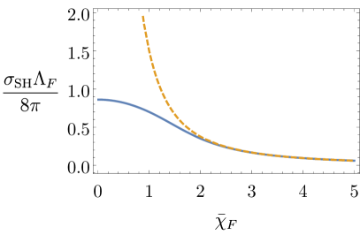
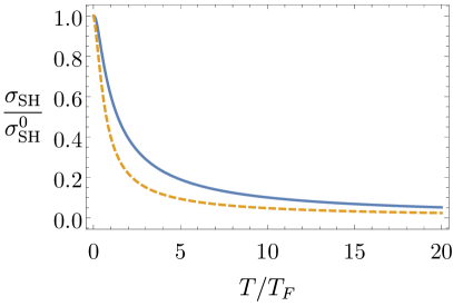
Figure 2: Left: dimensionless spin Hall conductivity as a function of the dimensionless SOC strength. Right: temperature dependence of spin Hall conductivity for a fixed SOC strength $\bar{\chi}_{F}=1$ normalized to spin Hall conductivity at low temperature. Both plots show the results for fermions (blue solid) and bosons (yellow dashed) in the absence of a condensate.

III.4 Validity of approximation

In our analysis we have applied the adiabatic approximation which is applicable when Eq. (13) holds. Here we explicitly check if this approximation holds for a typical experimental system in the range of interest of the parameters. Given a sufficiently low temperature and particle density, when only the bottom of the lowest band is occupied, we can assume that $|\boldsymbol{p}|\simeq\chi$. Moreover, we assume for clarity that the driving is provided by some harmonic potential with the displacement of the center of the system equal to the length of the trap. In that case Eq. (13) immediately yields the condition $\omega\beta_{F}\ll\bar{\chi}_{F}^{2}$, where $\omega$ is the trap frequency. We consider a system with a particle density of $10^{18}$m^-3, which corresponds to $T_{F}\simeq 20$nK. For these parameter values, a driving force provided by a $\omega=10$Hz trap leads to the adiabaticity criterion $\bar{\chi}_{F}\gg 0.1$.

Hence, our approximation is certainly valid in a setting when driving is relatively gentle, temperature is very low, and SOC strength is moderate. This regime, where $\sigma_{\text{SH}}$ is maximized and the approximation is robust, does not seem to put any extra challenges to the experimentalist, besides achieving the Weyl SOC. We note that temperatures as low as several nanokelvin have been demonstrated Medley et al. (2011), while an optically-generated SOC routinely achieves $\bar{\chi}_{F}=5$ in the equal Rashba-Dresselhaus case Beeler et al. (2013). The question of validity of the adiabatic approximation is, however, separate from the feasibility of detecting this effect. The latter question is addressed in the next subsection.

In applying our adiabatic approximation we have implicity assumed that the driving is switched on slowly. However, if the driving is switched on suddenly, the adiabatic approximation is not sufficient, and one has to solve the LLE at least to the second order in time derivatives. We have checked, however, that the SHE is still present in this post-adiabatic solution. The only new feature that arises in this higher-order solution is a Zitterbewegung-like beating between the two adiabatic solutions, which has been considered elsewhere Vaishnav and Clark (2008); Merkl et al. (2008); Qu et al. (2013); LeBlanc et al. (2013); Zülicke et al. (2007).

III.5 Detection of spin current

As discussed above, the most direct signature of the omnidirectional Hall effect is the spin current $\delta J_{\text{spin}}$. The experimental sequence needed to detect that current depends on the precise details of the implementation of Weyl SOC, as proposals to achieve it utilize qualitatively different physical means Anderson et al. (2012, 2013); Anderson and Clark (2013). Nevertheless, several general remarks can be made with no reference to these experimental details.

In particular, it is possible to utilize the fact that $\delta J_{\text{spin}}$ given by Eq. (21) is the transverse spin current. This is beneficial, since the equilibrium spin current $J^{0}_{\text{spin}}$ is longitudinal, and the spin of an atom in the upper (lower) band points along (opposite to) the momentum $\boldsymbol{p}$. As a result, one can filter out the $\delta J_{\text{spin}}$ signal by choosing a beneficial configuration of the driving direction $\boldsymbol{e}_{\beta}$, the spin (Stern-Gerlach) projection axis $\boldsymbol{e}_{j}=\boldsymbol{e}_{\text{SG}}$ and the direction of the momentum measurement $\boldsymbol{e}_{j}=\boldsymbol{e}_{\text{det}}$. Specifically, if one takes these three vectors to be orthogonal, the triple product

$$\boldsymbol{e}_{\text{det}}\cdot(\boldsymbol{e}_{\text{SG}}\times\boldsymbol{e}_{\beta})$$ (33)

featured in Eq. (21) for $\delta J_{\text{spin}}$ is maximized and the signal is the strongest. A relation between the spin current and the spin (Stern-Gerlach) projection measurement is considered in the last subsection of the Appendix.

Moreover, one can estimate the size of the effect of the omnidirectional spin Hall effect on the momentum distribution. Since the SOC strength $\chi$ sets the characteristic momentum in the distribution of particles in the system, the magnitude of the signal (the change of the momentum distribution due to the omnidirectional spin Hall effect) is approximately equal to the ratio $\dot{\beta}\sigma_{\text{SH}}/\nu\chi$.

III.6 Spin-current induced by a time-dependent Zeeman term

The spin Hall effect can also be induced by a time-dependent Zeeman shift rather than by a time-dependent external force. In that case the term $\gamma\boldsymbol{e}_{\gamma}\cdot\hat{\boldsymbol{\sigma}}$ is to be added to the Hamiltonian, and the effective magnetic field $\boldsymbol{M}$ determining the spin dynamics becomes

$$\boldsymbol{M}=\chi\boldsymbol{p}/m+\gamma\boldsymbol{e}_{\gamma}\,.$$ (34)

Since the scalar driving $\beta$ (due to a spin-independent force on an atom), and the Zeeman driving $\gamma$ (due to a magnetic pulse) enter the effective magnetic field $\boldsymbol{M}$ in the same manner, these two ways of driving the system lead to the same effect for the spin dynamics. Therefore, the above analysis of the induced spin current due to the spin-independent force can be transferred in a straightforward manner to the case of the Zeeman driving via the replacement of $\beta$ by $-m\gamma$ and $\boldsymbol{e}_{\beta}$ by $\boldsymbol{e}_{\gamma}$.

IV Summary and future work

In summary, we have put forward a proposal to observe inherently non-Abelian dynamics in the form of an omnidirectional spin Hall effect in a driven system in the presence of a Weyl (three-dimensional) spin-orbit coupling. We have discussed two independent ways to drive the system leading to the same effect for the spin dynamics: either through a constant spin-independent force or a time-dependent Zeeman field. We have also evaluated the strength of this effect in terms of conductivity for noninteracting uncondensed bosonic or fermionic gas. All of the components of this proposal seem to be within the reach of cold-atom experiments in the near future, and their combination has a potential to unambiguously demonstrate non-Abelian dynamics in a continuum (non-lattice) cold-atom system for the first time.

In future work, we plan to investigate collective modes of a trapped system and look for signatures of the non-Abelian dynamics described here. Other promising avenues of research include a more careful account of interactions, especially with the Bose-Einstein condensation in mind, and also considering the kinetic effects in this system, e.g., the relaxation of spin current also known as spin drag Koller et al. (2015), which was not considered here.

*

Appendix A Spin current

In this Appendix we motivate the definition of the spin current given in the text by deriving the spin continuity equation and considering the effect of a spin (Stern-Gerlach) projection on the velocity operator. In contrast to the main text, in this Appendix we use hats to label not only the spin operators but all operators (including the coordinate and momentum operators $\hat{\boldsymbol{r}}$ and $\hat{\boldsymbol{p}}$) in order to make the Appendix as accessible as possible.

A.1 Continuity equation and spin current

The spin density is a vector field given by

$$\boldsymbol{\rho}(\boldsymbol{r})=\Psi^{{\dagger}}(\boldsymbol{r})\hat{\boldsymbol{\sigma}}\Psi(\boldsymbol{r})=\langle\Psi|\boldsymbol{r}\rangle\hat{\boldsymbol{\sigma}}\langle\boldsymbol{r}|\Psi\rangle=\langle\Psi|\hat{\boldsymbol{\rho}}_{\boldsymbol{r}}|\Psi\rangle\,,$$ (35)

where $\hat{\boldsymbol{\rho}}_{\boldsymbol{r}}=\hat{\boldsymbol{\sigma}}\delta(\hat{\boldsymbol{r}}-\boldsymbol{r})$ is the corresponing spin density operator, and $\Psi(\boldsymbol{r})=\langle\boldsymbol{r}|\Psi\rangle$ is a two component column-spinor. Here the quantum average has been carried out over the full state-vector $|\Psi\rangle$ accommodating both the motional and spin degrees of the atom. Furthermore, we have casted the operator $\delta(\hat{\boldsymbol{r}}-\boldsymbol{r})=|\boldsymbol{r}\rangle\langle\boldsymbol{r}|$ in terms of the eigenstates $|\boldsymbol{r}\rangle$ of the coordinate operator: $\hat{\boldsymbol{r}}|\boldsymbol{r}\rangle=\boldsymbol{r}|\boldsymbol{r}\rangle$.

The dynamics of the operator $\hat{\boldsymbol{\rho}}_{\boldsymbol{r}}$ is governed by the Hamiltonian given by Eq. (1) which contains the Weyl SOC term, and thus

$$\frac{d}{dt}\hat{\boldsymbol{\rho}}_{\boldsymbol{r}}= \frac{1}{i}[\hat{\boldsymbol{\rho}}_{\boldsymbol{r}},\hat{H}]$$ (36)

$$= \frac{1}{2}\sum_{l}\left(\frac{1}{i}[\hat{\boldsymbol{\rho}}_{\boldsymbol{r}},\hat{p}_{l}-\hat{\mathcal{A}}_{l}]\hat{v}_{l}+\hat{v}_{l}\frac{1}{i}[\hat{\boldsymbol{\rho}}_{\boldsymbol{r}},\hat{p}_{l}-\hat{\mathcal{A}}_{l}]\right)\,,$$

where the matrix-valued velocity operator $\hat{\boldsymbol{v}}$ is defined in Eq. (3). Since

$$[\hat{\boldsymbol{\rho}}_{\boldsymbol{r}},\hat{p}_{l}-\hat{\mathcal{A}}_{l}]=-i\boldsymbol{\sigma}\nabla_{l}\delta(\hat{\boldsymbol{r}}-\boldsymbol{r})-[\boldsymbol{\sigma},\hat{\mathcal{A}}_{l}]\delta(\hat{\boldsymbol{r}}-\boldsymbol{r})\,,$$

one arrives at the following continuity equation:

$$\frac{d}{dt}\hat{\boldsymbol{\rho}}_{\boldsymbol{r}}+\nabla_{l}\hat{\boldsymbol{j}}_{\boldsymbol{r}l}=\hat{\mathbf{G}}_{\boldsymbol{r}}\,,$$ (37)

where

$$\hat{\mathbf{G}}_{\boldsymbol{r}}=-\frac{1}{2i}\left(\delta(\hat{\boldsymbol{r}}-\boldsymbol{r})[\hat{\boldsymbol{\sigma}},\hat{\mathcal{A}}_{l}]\hat{v}_{l}+\hat{v}_{l}[\hat{\boldsymbol{\sigma}},\hat{\mathcal{A}}_{l}]\delta(\hat{\boldsymbol{r}}-\boldsymbol{r})\right)$$ (38)

is the spin source operator and

$$\hat{\boldsymbol{j}}_{\boldsymbol{r}l}=\frac{1}{2}(\delta(\hat{\boldsymbol{r}}-\boldsymbol{r})\hat{\boldsymbol{\sigma}}\hat{v}_{l}+\hat{v}_{l}\hat{\boldsymbol{\sigma}}\delta(\hat{\boldsymbol{r}}-\boldsymbol{r}))$$ (39)

is the probability current operator.

In what follows we shall consider the spin current for momentum eigenstates of the Weyl SOC Hamiltonian,

$$\Psi(\boldsymbol{r})=\Psi_{\mathbf{p}\pm}(\boldsymbol{r})=V^{-1/2}\eta_{\mathbf{p}\pm}e^{i\mathbf{p}\cdot\mathbf{r}}\,,$$ (40)

where $V$ is a quantization volume and the spinor $\eta_{\mathbf{p}\pm}$ describes the quantum states for the spin along or opposite to the momentum: $\mathbf{p}/p\cdot\hat{\boldsymbol{\sigma}}\eta_{\mathbf{p}\pm}=\mp\eta_{\mathbf{p}\pm}$. The corresponding expectation value of the spin current is

$$\boldsymbol{j}_{l}(\boldsymbol{r})=\left\langle\Psi\right|\hat{\boldsymbol{j}}_{\boldsymbol{r}l}|\Psi\rangle=\frac{1}{2V}\langle\{\hat{\boldsymbol{\sigma}},\hat{v}_{l}\}\rangle\,,$$ (41)

with $\{\hat{\boldsymbol{\sigma}},\hat{v}_{l}\}=\hat{\boldsymbol{\sigma}}\hat{v}_{l}+\hat{v}_{l}\hat{\boldsymbol{\sigma}}$, where the brackets $\langle\cdots\rangle$ label the quantum averaging over the spinor state $\eta_{\mathbf{p}\pm}$. Performing also a statistical averaging over the atomic single-particle distribution $f^{\pm}(\mathbf{p})$, one arrives at the spin current presented in Eq. (15) of the main text:

$$(J_{\text{spin}})_{i}^{j}=\sum_{\boldsymbol{p},\eta=\pm}\frac{f^{\eta}(\boldsymbol{p})}{2V}\langle\{\hat{\sigma}_{j},\hat{v}_{i}\}\rangle=\frac{1}{2}\overline{\langle\{\hat{\sigma}_{j},\hat{v}_{i}\}\rangle}\,,$$ (42)

where the statistical averaging is denoted by an overline.

A.2 Source term

The vector potential $\hat{\mathbfcal{A}}$ given by Eq. (1) describes the 3D SOC and the driving. The space- and spin-independent driving term $\beta(t)\mathbf{e}_{\beta}$ does not contribute to the commutators entering Eq. (38), giving

$$[\hat{\sigma}_{j},\hat{\mathcal{A}}_{l}]\hat{v}_{l}=\chi[\hat{\sigma}_{j},\hat{\sigma}_{l}]\hat{v}_{l}=2i\chi\varepsilon_{jln}\hat{\sigma}_{n}\hat{v}_{l}=-2i\chi(\boldsymbol{\hat{\sigma}}\times\hat{\boldsymbol{v}})_{j}\,.$$ (43)

In a similar way,

$$\hat{v}_{l}[\hat{\sigma}_{j},\hat{\mathcal{A}}_{l}]=2i\chi(\hat{\boldsymbol{v}}\times\boldsymbol{\hat{\sigma}})_{j}\,.$$ (44)

Consequently,

$$\hat{\mathbf{G}}_{\boldsymbol{r}}=\chi\left(\delta(\hat{\boldsymbol{r}}-\boldsymbol{r})\hat{\boldsymbol{\sigma}}\times\hat{\boldsymbol{v}}-\hat{\boldsymbol{v}}\times\hat{\boldsymbol{\sigma}}\delta(\hat{\boldsymbol{r}}-\boldsymbol{r})\right)\,.$$ (45)

with $m\hat{\boldsymbol{v}}=\hat{\boldsymbol{p}}-\chi\hat{\boldsymbol{\sigma}}-\beta\mathbf{e}_{\beta}$.

In the case of the 3D SOC, the eigenstates $\eta_{\mathbf{p}\pm}$ describe the spin along the momentum: $\langle\hat{\boldsymbol{\sigma}}\rangle=\pm\mathbf{p}/p$ . Therefore, the source term vanishes after taking the quantum expectation value $\langle\hat{\mathbf{G}}_{\boldsymbol{r}}\rangle$ and averaging over an isotropic momentum distribution.

A.3 Spin projection measurement

Here we consider the effect of the spin (Stern-Gerlach) projection measurement on the velocity $\hat{v}_{i}$ along the unit vector $\boldsymbol{e}_{i}$. We will show that the spin current measured in this way is consistent with its previous definition. In particular, a Stern-Gerlach (SG) projection in the $j$ direction is given by the projector $|s_{j}\rangle\langle s_{j}|$, where the quantum state $|s_{j}\rangle$ describes the spin pointing along the unit vector $\boldsymbol{e}_{j}$. Calculating the expectation value of the velocity operator $\hat{v}_{i}$ with respect to such spin-projected states entails evaluating $|s_{j}\rangle\langle s_{j}|\hat{v}_{i}|s_{j}\rangle\langle s_{j}|$. Since the spin projection operator can be written down as

$$\hat{I}_{s_{j}}=|s_{j}\rangle\langle s_{j}|=\frac{1}{2}(1+\boldsymbol{e}_{j}\cdot\hat{\boldsymbol{\sigma}}),$$ (46)

we have

$$\hat{I}_{s_{j}}\hat{v}_{i}\hat{I}_{s_{j}}=\big{(}\hat{v}_{i}+\left(\boldsymbol{e}_{j}\cdot\hat{\boldsymbol{\sigma}}\right)\hat{v}_{i}\left(\boldsymbol{e}_{j}\cdot\hat{\boldsymbol{\sigma}}\right)\big{)}/4\\ +\big{(}\left(\boldsymbol{e}_{j}\cdot\hat{\boldsymbol{\sigma}}\right)\hat{v}_{i}+\hat{v}_{i}\left(\boldsymbol{e}_{j}\cdot\hat{\boldsymbol{\sigma}}\right)\big{)}/4.$$ (47)

Comparing this expression with Eq. (15), one can see that the second term on the right-hand side is proportional to the spin current. Using the properties of Pauli matrices, the first term simplifies to

$$\hat{v}_{i}+\left(\boldsymbol{e}_{j}\cdot\hat{\boldsymbol{\sigma}}\right)\hat{v}_{i}\left(\boldsymbol{e}_{j}\cdot\hat{\boldsymbol{\sigma}}\right)\\ =2\left[p_{i}-\chi\left(\boldsymbol{e}_{j}\cdot\hat{\boldsymbol{\sigma}}\right)\left(\boldsymbol{e}_{i}\cdot\boldsymbol{e}_{j}\right)\right]/m.$$ (48)

Consequently

$$\hat{I}_{s_{j}}\hat{v}_{i}\hat{I}_{s_{j}}=\frac{p_{i}-\chi\left(\boldsymbol{e}_{j}\cdot\hat{\boldsymbol{\sigma}}\right)\left(\boldsymbol{e}_{i}\cdot\boldsymbol{e}_{j}\right)}{2m}+\frac{(\hat{J}_{\text{spin}})_{i}^{j}}{2}\,.$$ (49)

As the projection direction is reversed, $\boldsymbol{e}_{j}\rightarrow-\boldsymbol{e}_{j}$, the first term is unaffected, while the second term changes its sign. Therefore by considering the difference in velocities between the spin up and the spin down components resulting from a spin (Stern-Gerlach) projection in the direction $\boldsymbol{e}_{j}$, one measures the spin current exactly as defined in Eq. (15) in the main text.

References

- Frankel (2004) T. Frankel, The Geometry of Physics: An Introduction (Cambridge University Press, 2004).
- Berry (1984) M. V. Berry, Proceedings of the Royal Society of London. A. Mathematical and Physical Sciences 392, 45 (1984).
- Shapere and Wilczek (1989) A. Shapere and F. Wilczek, eds., Geometric Phases in Physics (World Scientific, Singapore, 1989).
- Bohm et al. (2003) A. Bohm, A. Mostafazadeh, H. Koizumi, Q. Niu, and J. Zwanziger, Geometric Phases in Quantum Systems (Springer, Berlin, Heidelberg, New York, 2003).
- Mead (1992) C. A. Mead, Rev. Mod. Phys. 64, 51 (1992).
- Loss et al. (1990) D. Loss, P. Goldbart, and A. V. Balatsky, Phys. Rev. Lett. 65, 1655 (1990).
- Lévy et al. (1990) L. P. Lévy, G. Dolan, J. Dunsmuir, and H. Bouchiat, Phys. Rev. Lett. 64, 2074 (1990).
- Chandrasekhar et al. (1991) V. Chandrasekhar, R. A. Webb, M. J. Brady, M. B. Ketchen, W. J. Gallagher, and A. Kleinsasser, Phys. Rev. Lett. 67, 3578 (1991).
- Mailly et al. (1993) D. Mailly, C. Chapelier, and A. Benoit, Phys. Rev. Lett. 70, 2020 (1993).
- Neubauer et al. (2009) A. Neubauer, C. Pfleiderer, B. Binz, A. Rosch, R. Ritz, P. G. Niklowitz, and P. Böni, Phys. Rev. Lett. 102, 186602 (2009).
- Li et al. (2013a) Y. Li, N. Kanazawa, X. Z. Yu, A. Tsukazaki, M. Kawasaki, M. Ichikawa, X. F. Jin, F. Kagawa, and Y. Tokura, Phys. Rev. Lett. 110, 117202 (2013a).
- Hasan and Kane (2010) M. Hasan and C. Kane, Rev. Mod. Phys. 82, 3045 (2010).
- Bliokh et al. (2008) K. Y. Bliokh, A. Niv, V. Kleiner, and E. Hasman, Nat. Photon. 2, 748 (2008).
- Hafezi et al. (2011) M. Hafezi, E. A. Demler, M. D. Lukin, and J. M. Taylor, Nature Phys. 7, 907 (2011).
- Kitagawa et al. (2013) T. Kitagawa, M. A. Broome, A. Fedrizzi, M. S. Rudner, E. Berg, I. Kassal, A. Aspuru-Guzik, E. Demler, and A. G. White, Nat. Commun. 3, 882 (2013).
- Rechtsman et al. (2013) M. C. Rechtsman, J. M. Zeuner, Y. Plotnik, Y. Lumer, D. Podolsky, F. Dreisow, S. Nolte, M. Segev, and A. Szameit, Nature 496, 196 (2013).
- Mittal et al. (2014) S. Mittal, J. Fan, S. Faez, A. Migdall, J. Taylor, and M. Hafezi, Phys. Rev. Lett. 113, 087403 (2014).
- Tzuang et al. (2014) L. D. Tzuang, K. Fang, P. Nussenzveig, S. Fan, and M. Lipson, Nat. Photon. 8, 701 (2014).
- Dubček et al. (2015) T. Dubček, K. Lelas, D. Jukić, R. Pezer, M. Soljačić, and H. Buljan, New J. Phys. 17, 125002 (2015).
- Skirlo et al. (2015) S. A. Skirlo, L. Lu, Y. Igarashi, Q. Yan, J. Joannopoulos, and M. Soljačić, Phys. Rev. Lett. 115, 253901 (2015).
- Ozawa et al. (2016) T. Ozawa, H. M. Price, N. Goldman, O. Zilberberg, and I. Carusotto, Phys. Rev. A 93, 043827 (2016).
- Süsstrunk and Huber (2015) R. Süsstrunk and S. D. Huber, Science 349, 47 (2015).
- Salerno et al. (2016) G. Salerno, T. Ozawa, H. M. Price, and I. Carusotto, Phys. Rev. B 93, 085105 (2016).
- Ningyuan et al. (2015) J. Ningyuan, C. Owens, A. Sommer, D. Schuster, and J. Simon, Phys. Rev. X 5, 021031 (2015).
- Albert et al. (2015) V. V. Albert, L. I. Glazman, and L. Jiang, Phys. Rev. Lett. 114, 173902 (2015).
- Wilczek and Zee (1984) F. Wilczek and A. Zee, Phys. Rev. Lett. 52, 2111 (1984).
- Zee (1988) A. Zee, Phys. Rev. A 38, 1 (1988).
- Zwanziger et al. (1990) J. W. Zwanziger, M. Koenig, and A. Pines, Phys. Rev. A 42, 3107 (1990).
- Lin et al. (2009a) Y.-J. Lin, R. L. Compton, A. R. Perry, W. D. Phillips, J. V. Porto, and I. B. Spielman, Phys. Rev. Lett. 102, 130401 (2009a).
- Lin et al. (2009b) Y. J. Lin, R. L. Compton, K. Jimenez-Garcia, J. V. Porto, and I. B. Spielman, Nature 462, 628 (2009b).
- Aidelsburger et al. (2011) M. Aidelsburger, M. Atala, S. Nascimbène, S. Trotzky, Y.-A. Chen, and I. Bloch, Phys. Rev. Lett. 107, 255301 (2011).
- Struck et al. (2012) J. Struck, C. Ölschläger, M. Weinberg, P. Hauke, J. Simonet, A. Eckardt, M. Lewenstein, K. Sengstock, and P. Windpassinger, Phys. Rev. Lett. 108, 225304 (2012).
- Aidelsburger et al. (2013) M. Aidelsburger, M. Atala, M. Lohse, J. T. Barreiro, B. Paredes, and I. Bloch, Phys. Rev. Lett. 111, 85301 (2013).
- Miyake et al. (2013) H. Miyake, G. A. Siviloglou, C. J. Kennedy, W. C. Burton, and W. Ketterle, Phys. Rev. Lett. 111, 185302 (2013).
- Kennedy et al. (2013) C. J. Kennedy, G. A. Siviloglou, H. Miyake, W. C. Burton, and W. Ketterle, Phys. Rev. Lett. 111, 225301 (2013).
- Armaitis et al. (2013) J. Armaitis, H. T. C. Stoof, and R. A. Duine, Phys. Rev. Lett. 110, 260404 (2013).
- Choi et al. (2013) J.-y. Choi, S. Kang, S. W. Seo, W. J. Kwon, and Y.-i. Shin, Phys. Rev. Lett. 111, 245301 (2013).
- Jotzu et al. (2014) G. Jotzu, M. Messer, R. Desbuquois, M. Lebrat, T. Uehlinger, D. Greif, and T. Esslinger, Nature 515, 237 (2014).
- Aidelsburger et al. (2014) M. Aidelsburger, M. Lohse, C. Schweizer, M. Atala, J. T. Barreiro, S. Nascimbène, N. R. Cooper, I. Bloch, and N. Goldman, Nature Phys. 11, 162 (2014).
- Atala et al. (2014) M. Atala, M. Aidelsburger, M. Lohse, J. T. Barreiro, B. Paredes, and I. Bloch, Nature Phys. 10, 588 (2014).
- Fläschner et al. (2016) N. Fläschner, B. S. Rem, M. Tarnowski, D. Vogel, D.-S. Lühmann, K. Sengstock, and C. Weitenberg, Science 352, 1091 (2016).
- Li et al. (2016) T. Li, L. Duca, M. Reitter, F. Grusdt, E. Demler, M. Endres, M. Schleier-Smith, I. Bloch, and U. Schneider, Science 352, 1094 (2016).
- Stuhl et al. (2015) B. K. Stuhl, H.-I. Lu, L. M. Aycock, D. Genkina, and I. B. Spielman, Science 349, 1514 (2015).
- Mancini et al. (2015) M. Mancini, G. Pagano, G. Cappellini, L. Livi, M. Rider, J. Catani, C. Sias, P. Zoller, M. Inguscio, M. Dalmonte, and L. Fallani, Science 349, 1510 (2015).
- Dudarev et al. (2004) A. M. Dudarev, R. B. Diener, I. Carusotto, and Q. Niu, Phys. Rev. Lett. 92, 153005 (2004).
- Ruseckas et al. (2005) J. Ruseckas, G. Juzeliūnas, P. Öhberg, and M. Fleischhauer, Phys. Rev. Lett. 95, 010404 (2005).
- Osterloh et al. (2005) K. Osterloh, M. Baig, L. Santos, P. Zoller, and M. Lewenstein, Phys. Rev. Lett. 95, 010403 (2005).
- Juzeliūnas et al. (2008) G. Juzeliūnas, J. Ruseckas, M. Lindberg, L. Santos, and P. Öhberg, Phys. Rev. A 77, 011802(R) (2008).
- Stanescu et al. (2007) T. D. Stanescu, C. Zhang, and V. Galitski, Phys. Rev. Lett. 99, 110403 (2007).
- Vaishnav and Clark (2008) J. Y. Vaishnav and C. W. Clark, Phys. Rev. Lett. 100, 153002 (2008).
- Liu et al. (2009) X.-J. Liu, M. F. Borunda, X. Liu, and J. Sinova, Phys. Rev. Lett. 102, 046402 (2009).
- Zhang (2010) C. Zhang, Phys. Rev. A 82, 021607(R) (2010).
- Campbell et al. (2011) D. L. Campbell, G. Juzeliūnas, and I. B. Spielman, Phys. Rev. A 84, 025602 (2011).
- Dalibard et al. (2011) J. Dalibard, F. Gerbier, G. Juzeliūnas, and P. Öhberg, Rev. Mod. Phys. 83, 1523 (2011).
- Anderson et al. (2012) B. M. Anderson, G. Juzeliūnas, V. M. Galitski, and I. B. Spielman, Phys. Rev. Lett. 108, 235301 (2012).
- Xu et al. (2013) Z.-F. Xu, L. You, and M. Ueda, Phys. Rev. A 87, 063634 (2013).
- Anderson et al. (2013) B. M. Anderson, I. B. Spielman, and G. Juzeliūnas, Phys. Rev. Lett. 111, 125301 (2013).
- Zhou et al. (2013) X. Zhou, Y. Li, Z. Cai, and C. Wu, J. Phys. B. 46, 134001 (2013).
- Anderson and Clark (2013) B. M. Anderson and C. W. Clark, J. Phys. B 46, 134003 (2013).
- Li et al. (2013b) Y. Li, G. I. Martone, L. P. Pitaevskii, and S. Stringari, Phys. Rev. Lett. 110, 235302 (2013b).
- Galitski and Spielman (2013) V. Galitski and I. B. Spielman, Nature 494, 49 (2013).
- Goldman et al. (2014) N. Goldman, G. Juzeliūnas, P. Öhberg, and I. B. Spielman, Rep. Prog. Phys. 77, 126401 (2014).
- Zhai (2015) H. Zhai, Rep. Prog. Phys. 78, 026001 (2015).
- Lin et al. (2011) Y.-J. Lin, K. Jiménez-García, and I. B. Spielman, Nature 471, 83 (2011).
- Zhang et al. (2012) J.-Y. Zhang, S.-C. Ji, Z. Chen, L. Zhang, Z.-D. Du, B. Yan, G.-S. Pan, B. Zhao, Y.-J. Deng, Z. H., S. Chen, and J.-W. Pan, Phys. Rev. Lett. 109, 115301 (2012).
- Wang et al. (2012) P. Wang, Z.-Q. Yu, Z. Fu, L. Miao, L. Huang, S. Chai, H. Zhai, and J. Zhang, Phys. Rev. Lett. 109, 095301 (2012).
- Cheuk et al. (2012) L. W. Cheuk, A. T. Sommer, Z. Hadzibabic, T. Yefsah, W. S. Bakr, and J. Zhang, Phys. Rev. Lett. 109, 095302 (2012).
- Williams et al. (2012) R. A. Williams, L. J. LeBlanc, K. Jiménez-García, M. C. Beeler, A. R. Perry, W. D. Phillips, and I. B. Spielman, Science 335, 314 (2012).
- LeBlanc et al. (2013) L. J. LeBlanc, M. C. Beeler, K. Jimenez-Garcia, A. R. Perry, S. Sugawa, R. A. Williams, and I. B. Spielman, New. J. Phys. 15, 073011 (2013).
- Qu et al. (2013) C. Qu, C. Hamner, M. Gong, C. Zhang, and P. Engels, Phys. Rev. A 88, 021604(R) (2013).
- Fu et al. (2014) Z. Fu, L. Huang, Z. Meng, P. Wang, L. Zhang, S. Zhang, H. Zhai, P. Zhang, and J. Zhang, Nature Phys. 10, 110 (2014).
- Huang et al. (2016) L. Huang, Z. Meng, P. Wang, P. Peng, S.-L. Zhang, L. Chen, D. Li, Q. Zhou, and J. Zhang, Nature Phys. 12, 540 (2016).
- Meng et al. (2016) Z. Meng, L. Huang, P. Peng, D. Li, L. Chen, Y. Xu, C. Zhang, P. Wang, and J. Zhang, Phys. Rev. Lett. 117, 235304 (2016).
- Wu et al. (2016) Z. Wu, L. Zhang, W. Sun, X.-T. Xu, B.-Z. Wang, S.-C. Ji, Y. Deng, S. Chen, X.-J. Liu, and J.-W. Pan, Science 354, 83 (2016).
- Ji et al. (2014) S.-C. Ji, J.-Y. Zhang, L. Zhang, Z.-D. Du, W. Zheng, Y.-J. Deng, H. Zhai, S. Chen, and J.-W. Pan, Nature Phys. 10, 314 (2014).
- Beeler et al. (2013) M. C. Beeler, R. A. Williams, K. Jiménez-García, L. J. LeBlanc, A. R. Perry, and I. B. Spielman, Nature 498, 201 (2013).
- Sinova et al. (2015) J. Sinova, S. O. Valenzuela, J. Wunderlich, C. H. Back, and T. Jungwirth, Rev. Mod. Phys. 87, 1213 (2015).
- Tokatly and Sherman (2016) I. V. Tokatly and E. Y. Sherman, Phys. Rev. A 93, 063635 (2016).
- Sinova et al. (2004) J. Sinova, D. Culcer, Q. Niu, N. A. Sinitsyn, T. Jungwirth, and A. H. MacDonald, Phys. Rev. Lett. 92, 126603 (2004).
- Burkov and Balents (2011) A. A. Burkov and L. Balents, Phys. Rev. Lett. 107, 127205 (2011).
- Ando (2013) Y. Ando, J. Phys. Soc. Jpn. 82, 102001 (2013).
- Borisenko et al. (2014) S. Borisenko, Q. Gibson, D. Evtushinsky, V. Zabolotnyy, B. Büchner, and R. J. Cava, Phys. Rev. Lett. 113, 027603 (2014).
- Liu et al. (2014) Z. Liu, B. Zhou, Y. Zhang, Z. Wang, H. Weng, D. Prabhakaran, S.-K. Mo, Z. Shen, Z. Fang, X. Dai, et al., Science 343, 864 (2014).
- Xu et al. (2015) S.-Y. Xu, C. Liu, S. K. Kushwaha, R. Sankar, J. W. Krizan, I. Belopolski, M. Neupane, G. Bian, N. Alidoust, T.-R. Chang, et al., Science 347, 294 (2015).
- Lu et al. (2015) L. Lu, Z. Wang, D. Ye, L. Ran, L. Fu, J. D. Joannopoulos, and M. Soljačić, Science 349, 622 (2015).
- Soluyanov et al. (2015) A. A. Soluyanov, D. Gresch, Z. Wang, Q. Wu, M. Troyer, X. Dai, and B. A. Bernevig, Nature 527, 495 (2015).
- Lv et al. (2015) B. Q. Lv, H. M. Weng, B. B. Fu, X. P. Wang, H. Miao, J. Ma, P. Richard, X. C. Huang, L. X. Zhao, G. F. Chen, Z. Fang, X. Dai, T. Qian, and H. Ding, Phys. Rev. X 5, 031013 (2015).
- Dubček et al. (2015) T. Dubček, C. J. Kennedy, L. Lu, W. Ketterle, M. Soljačić, and H. Buljan, Phys. Rev. Lett. 114, 225301 (2015).
- Wan et al. (2011) X. Wan, A. M. Turner, A. Vishwanath, and S. Y. Savrasov, Phys. Rev. B 83, 205101 (2011).
- Gürsoy et al. (2013) U. Gürsoy, V. Jacobs, E. Plauschinn, H. Stoof, and S. Vandoren, J. High Energy Phys. 2013, 1 (2013).
- Dimitrova (2005) O. V. Dimitrova, Phys. Rev. B 71, 245327 (2005).
- Khaetskii (2006) A. Khaetskii, Phys. Rev. Lett. 96, 056602 (2006).
- Leggett (2001) A. J. Leggett, Rev. Mod. Phys. 73, 307 (2001).
- Chin et al. (2010) C. Chin, R. Grimm, P. Julienne, and E. Tiesinga, Rev. Mod. Phys. 82, 1225 (2010).
- Guan and Blume (2017) Q. Guan and D. Blume, Phys. Rev. A 95, 020702 (2017).
- Fujita et al. (2011) T. Fujita, M. B. A. Jalil, S. G. Tan, and S. Murakami, J. Appl. Phys. 110, 121301 (2011).
- Landau and Lifshitz (1935) L. D. Landau and E. Lifshitz, Phys. Z. Sowjetunion 8, 101 (1935).
- Gilbert (2004) T. Gilbert, IEEE Trans. Magn. 40, 3443 (2004).
- Gaunt et al. (2013) A. L. Gaunt, T. F. Schmidutz, I. Gotlibovych, R. P. Smith, and Z. Hadzibabic, Phys. Rev. Lett. 110, 200406 (2013).
- van der Bijl and Duine (2011) E. van der Bijl and R. A. Duine, Phys. Rev. Lett. 107, 195302 (2011).
- Huang (2016) X.-G. Huang, Sci. Rep. 6, 20601 (2016).
- Rashba (2003) E. I. Rashba, Phys. Rev. B 68, 241315(R) (2003).
- Drouhin et al. (2011) H.-J. Drouhin, G. Fishman, and J.-E. Wegrowe, Phys. Rev. B 83, 113307 (2011).
- Sherman and Sokolovski (2014) E. Y. Sherman and D. Sokolovski, New J. Phys. 16, 015013 (2014).
- Tokatly (2008) I. V. Tokatly, Phys. Rev. Lett. 101, 106601 (2008).
- Phuc et al. (2015) N. T. Phuc, G. Tatara, Y. Kawaguchi, and M. Ueda, Nat. Commun. 6 (2015).
- Stanescu et al. (2008) T. D. Stanescu, B. Anderson, and V. Galitski, Phys. Rev. A 78, 023616 (2008).
- Medley et al. (2011) P. Medley, D. M. Weld, H. Miyake, D. E. Pritchard, and W. Ketterle, Phys. Rev. Lett. 106, 195301 (2011).
- Merkl et al. (2008) M. Merkl, F. E. Zimmer, G. Juzeliūnas, and P. Öhberg, EPL 83, 54002 (2008).
- Zülicke et al. (2007) U. Zülicke, J. Bolte, and R. Winkler, New J. Phys. 9, 355 (2007).
- Koller et al. (2015) S. B. Koller, A. Groot, P. C. Bons, R. A. Duine, H. T. C. Stoof, and P. van der Straten, New J. Phys. 17, 113026 (2015).