Lattice gas automaton modelling of a vortex flow meter: Strouhal-Reynolds number dependence

Abstract

Motivated by recent experimental and computational results concerning the three-dimensional structure of vortices behind a vortex shedding flow meter [M. Reik et al., Forsch. Ingenieurwes. 74, 77 (2010)], we study the Strouhal-Reynolds number dependence in the vortex street in two dimensions behind a trapezoid-shaped object by employing two types of Frisch-Hasslacher-Pomeau (FHP) models. Our geometry is intended to reproduce the operation of the vortex shedding flow meter in a two-dimensional setting, thus preventing the formation of three-dimensional vortex structure. In particular, we check if the anomalous Reynolds-Strouhal number dependence reported for three dimensions can also be found in our two-dimensional simulation. As we find that the Strouhal number is nearly independent of the Reynolds number in this particular setup, our results provide support for the hypothesis that three-dimensional flow structures are responsible for that dependence, thus hinting at the importance of the pipe diameter to the accurate operation of industrial vortex flow meters.

I Introduction

Hydrodynamic theories have been studied for a long time, but they still provide new insights in various problems of physics and engineering, from nondissipative currents in ultracold atomic vapour book:pitaevskii to stability of tall buildings article:irwin_2010 , in addition to posing some extremely challenging questions along the way link:claymath . Several branches of the field remain particularly vigorous, including studies of flow instabilities book:sengupta . Besides being of fundamental importance, flow instabilities in general, and the renowned Kármán vortex street article:mallock ; article:benard in particular can be readily observed in everyday life book:karman , and also has important practical uses.

The vortex shedding flow meter stands out as a direct industrial application of the phenomenon of the Kármán vortex street. This device consists of a blunt object positioned inside a pipe, and a detector of vortices. As liquid (or gas) flows through the pipe sufficiently fast, a vortex street forms downstream from the blunt object. Since the vortex shedding frequency is dependent on the hydrodynamic properties of the flow, the signal of the vortex detector can be converted to the velocity measurement of the flow. This type of a device is uniquely suitable for operation in an industrial setting, as it is fully contained inside the pipe, has no moving parts, and is both robust and reliable book:boyes .

It turns out that even in this seemingly mundane setting of a tested industrial application, novel physics can be uncovered. In particular, it has been recently suggested that the vortex pattern that forms downstream from the vortex flow meter has a three-dimensional structure article:reik_et_al_2010 , in the shape of so-called horseshoe vortices. In turn, this spatial structure alters the flow in the pipe, introducing an anomalous relation between the Reynolds and the Strouhal numbers. This anomalous relation violates the main operating assumption of the flow meter, therefore leading to inaccurate flow measurements in certain regimes. In this paper, we provide an additional check if the spatial structure is indeed to blame for the anomalous relation by numerically studying the same problem in a two-dimensional geometry, where the horseshoe vortices cannot form.

The traditional approach to hydrodynamics, namely solving the Navier-Stokes equations, is considered to be both analytically and computationally complicated. Analytical solutions of hydrodynamic problems are possible only in limited number of cases of flows at small Reynolds numbers and in relatively simple geometries. Some hydrodynamic instabilities can be investigated analytically and numerically using dynamical systems approaches. For example, expansion around instabilities may result in equations that are simpler than Navier-Stokes equations, but which are nevertheless able to reproduce the formation of hydrodynamic patterns book:ds_appr_turb_1998 ; book:hydro_instab_trans_turb_1981 . Also, in some cases, weakly or moderately turbulent flows can be described using the so-called shell models that consist in replacing the partial differential equation with a system of coupled ordinary differential equations via discretization and truncation in Fourier space book:ds_appr_turb_1998 . However, for extremely high Reynolds numbers, because of the large number of relevant degrees of freedom due to the wide range of scales, the traditional descriptions of fully developed turbulence employ statistical methods book:monin1 ; book:monin2 and phenomenological models article:kolmogorov41 ; article:kolmogorov62 .

An altogether different approach to hydrodynamic problems are the so-called lattice gas models review:wolfram ; book:lattice-gas_hydro_2001 ; thesis:wylie_1990 . These models belong to a wide class of discrete systems known as cellular automata. They have a direct physical interpretation. Namely, point particles occupy nodes of a lattice with the possibility to jump from one node to one of its neighbouring nodes in a single time step. In most of these models the particles move with a single speed in one of several directions. Collisions of the particles occur at the nodes, and are executed according to some simple logical rules. Remarkably, if the lattice has proper symmetries and the collision rules satisfy relevant conservation laws (e.g., momentum and energy conservation), then the global behaviour of the system in a coarse-grained picture will closely resemble the flow of a fluid book:lattice-gas_hydro_2001 ; article:fhp .

In this work, two different rule sets of the seven-particle Frisch-Hasslacher-Pomeau (FHP, article:fhp ) model have been used in order to simulate the vortex flow meter article:reik_et_al_2010 . These FHP models have been successfully employed to attack diverse problems, including nucleation in supersaturated liquids article:hickey , sand dune growth article:gao , as well as flows on curved surfaces with dynamical geometry article:klales , in addition to shedding insight on various aspects of hydrodynamics book:lattice-gas_hydro_2001 . Hence, even though more elaborate methods to address fluid dynamics are present (for example, the lattice Boltzmann equation book:succi ), in our case we have employed the FHP lattice gas model in order to minimize the computation effort, while still obtaining reliable results.

The structure of the paper is as follows. Section II introduces the FHP lattice gas models used for the simulations, together with the definitions of Reynolds and Strouhal numbers in this framework. Then, in Section III, the main results are presented and discussed. Finally, Section IV summarizes the results and draws some conclusions, in addition to discussing several promising directions for future investigations.

II Methods of simulation

In this section we briefly describe the lattice gas automata in general, and the FHP models in particular. Even though several excellent resources on these subjects are available (see, e.g., Refs. book:lattice-gas_hydro_2001 and thesis:wylie_1990 as well as the references within them), we summarize the most important aspects of the methods employed in order to make our discussion self-contained.

The lattice gas automata consist of discrete nodes arranged geometrically in a Bravais lattice thesis:wylie_1990 ; book:lattice-gas_hydro_2001 ; review:dHumieres_Lallemand . Since the number of nodes is finite, suitable boundary conditions (most commonly, periodic) must be implemented. Each node has a fixed number of channels that can be either empty or occupied by a single particle. The channels point to the nearest neighbouring nodes, therefore a particle in each channel is considered to possess a single speed in the direction of the neighbouring node to which that channel is pointing.

The time evolution proceeds in discrete steps where each single step consists of two phases – propagation and collision. During the propagation phase, the particles move, i.e. the occupied state of a channel in each node is transferred to the channel of the same direction in the corresponding neighbouring node. In the collision phase, the states of each node change locally, according to a set of fixed rules. In order to reproduce the macroscopic properties of a physical fluids, the collision rules and lattice geometry are constructed in such a way that the relevant conservation laws and certain symmetries remain in tact.

The rigid obstacles and impermeable boundaries are introduced by setting up special collision rules describing particle reflection for the nodes at the boundaries. Also the sources and sinks may be added by special rules of particle creation/destruction at some nodes.

II.1 The FHP models

The FHP models article:fhp belong to a class of two-dimensional lattice gas models based on the two-dimensional triangular lattice. There are several versions of the FHP models that maintain the same lattice structure, but differ in collision rules.

The simplest version is the so-called FHP-I model where each node has 6 channels corresponding to the 6 directions on the triangular lattice. For our simulations we have used the FHP-II and FHP-III versions where 7 particles at each node may exist – six moving and one additional particle at rest (having zero velocity). Besides having a higher number of possible effective collisions, the main feature of the FHP-III model compared to FHP-I and FHP-II models is the property of self-duality. This means that the dynamics of particles (occupied channels) is equivalent to the dynamics of holes (unoccupied channels) and the dynamics, i.e., the collision rules for the dual states (with occupied and unoccupied channels exchanged) are the same as for the original states.

II.2 Averaging and macroscopic observables

The discrete dynamics of the states of nodes on the Bravais lattice described above constitutes the microscopic dynamics of the model with microscopic quantities, such as local density (number of particles at the node), velocities of particles (or local velocity field taken as an average velocity of all particles at the given node). These quantities have little to do with actual microscopic dynamics that takes place in real physical fluids. However, under appropriate circumstances, the macroscopic properties of the lattice gas can reproduce the macroscopic properties of real fluids.

The macroscopic observables from the lattice gas simulations are obtained by spatial and temporal averaging. Spatial averaging consists in averaging the microscopic states over blocks of nodes. Temporal averaging means that the value of the state is taken averaged over multiple time steps.

Here we have used spatial averaging over $16\times 16$ blocks of nodes and for the velocity field. Also, temporal averaging over 10 time steps has been used unless noted otherwise.

II.3 Reynolds and Strouhal numbers

Reynolds number is a dimensionless number that characterizes the flow by showing the relative importance of inertial and viscous forces book:landau_hydro_1987 . It is widely used to quantitatively describe different regimes of the flow.

For the FHP-III model, the Reynolds number $Re$ is calculated in the following way book:lattice-gas_hydro_2001 . First, the density $\rho$ of the particles on the lattice is measured. Since it is a number from 0 to 7 for each node, it is convenient to use the reduced density $d=\rho/7$. Because of the self-duality of the FHP-III model, if $d>0.5$, then the dynamics of holes instead of particles is being observed, therefore $d\equiv 1-d$ in that case. Because of this, certain macroscopic observables differ from theoretical ones by the density dependent non-Galilean factor book:lattice-gas_hydro_2001 :

$$g(d)=\frac{7}{12}\frac{1-2d}{1-d}\,\,.$$ (1)

Another important quantity required in order to calculate $Re$ is the kinematic viscosity:

$$\eta=\frac{1}{28d\bar{d}(1-\frac{8}{7}d\bar{d})}-\frac{1}{8}$$ (2)

where $\bar{d}=1-d$. The Reynolds number is

$$Re=\frac{guL}{\eta}\,\,.$$ (3)

where $u$ is the average velocity magnitude and $L$ is the typical dimension of the obstacle. One readily notices, that in order to increase $Re$, one has to choose a wide channel, produce high velocity of the flow and optimize $d$. In the present case $Re$ is maximized at $d\cong 0.305$.

The Strouhal number $St$ is another dimensionless quantity, characterizing the flow. The function $St(Re)$ provides important information about what is happening at the wake book:lattice-gas_hydro_2001 . It is defined by the following equation:

$$St=\frac{f\cdot L}{u\cdot g}\,\,,$$ (4)

where $L$ is again the typical size of the obstacle (in this case, the length of the base of the triangle, see Fig. 3). $f$ is the frequency of the wake oscillation produced by vortex shedding. All the quantities are in natural lattice units (i.e. number of lattice sites and time steps).

The industrial vortex flow meters function under the assumption of constant $St$. If this were the case, the frequency $f$ of the vortex shedding would depend linearly on the flow velocity $u$. However this turns out not to be true at least in some regimes of the flow article:reik_et_al_2010 .

In our case $f$ is determined by the lattice gas hot-wire anemometry book:lattice-gas_hydro_2001 – averaging over a block where the local velocity magnitude is recorded at each step. Later on, Fourier analysis and sine function fitting is used to determine the low frequency mode from the noisy signal, since a direct application of the FFT is often not a good option, as it requires many steps to obtain reasonably small errors due to fluctuations of the velocity field, which in turn come about due to complex flow patterns. The low frequency mode in the case of Kármán vortex street corresponds to the vortex shedding frequency. A piece of raw data and the corresponding sine function fit are provided in Fig. 4.

III Simulation of a vortex flow meter

Even though there is a considerable body of knowledge concerning vortex formation in flows behind cylinders roshko , and other highly symmetric objects in translationally-invariant geometries, the particular case of a prism in a confined setting has not been studied yet up to the best of our knowledge. Since the main goal of this paper is to simulate the vortex flow meter that is usually placed in a pipe, as in article:reik_et_al_2010 , periodic boundary conditions have been used in the $x$ direction being main direction of the flow (from the left to to the right in the figures), and the containment of the flow by the pipe walls has been implemented as impermeable boundaries from the top and the bottom (i.e., in $y$ direction).

This section presents results from a series of simulations in several different geometries. First, the velocity profile of the steady flow without an obstacle has been obtained in order to test the velocity profile (Fig. 1). Then, the vortex shedding from a triangle has been implemented and visualized in both FHP-II and FHP-III models (Fig. 2). Finally, the two-dimensional model of a vortex flow meter has been simulated by placing the blunt prism-shaped vortex shedding device (Fig. 3) in the flow with two different ratios of obstacle size to channel width in order to measure the dependence of the vortex shedding frequency on the flow velocity and determine the Strouhal-Reynolds number dependence (Fig. 5 and Fig. 6).

III.1 Velocity profile of the laminar flow

Before starting the simulation of unsteady flow of the vortex street behind an obstacle, the velocity profile of an unobstructed flow has been investigated using the FHP-II model. On a lattice of $120\times 48$ cells (each cell, as mentioned before, being a block of $16\times 16$ nodes) the velocity component $v_{x}$ along the general flow direction has been measured. A steady-state velocity profile has been determined for every horizontal block of cells (coordinate $y$ ranging from 1 to 48) by spatial averaging of the velocity over cells 40 to 100 in the $x$ direction and temporal averaging over 100 time steps. Two mechanisms of flow induction have been considered.

First, the so-called fan approach thesis:wylie_1990 has been implemented. This approach consists of a vertical zone of $1\times 48$ cells where each particle moving to the left (in the opposite direction to $x$) is being reversed with probability $0.001$. Using this approach, however, an almost rectangular velocity profile has been observed (left panel of Fig. 1), instead of the expected Poiseuille profile book:monin1 .

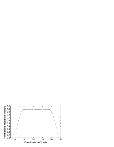
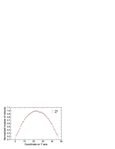
Figure 1: Left panel: rectangular velocity profile resulting from the fan approach. Right panel: velocity profile in the source/sink case. Circles represent the measured data, and the solid red line is the Poiseuille profile fit.

Next, we have used the source/sink flow induction mechanism. A source or a sink is a node where each arriving particle is absorbed (destroyed) and new particles moving in all the available directions (6 in the FHP case) are introduced each with some probability thesis:wylie_1990 . If, for example, this probability is $0.2$, then $6\times 0.2=1.2$ particles at the source/sink node are created on average. If, on average, there are more particles produced than destroyed, then such a node acts as a source, and, if there are more particles destroyed than created, a node acts as a sink.

We have implemented the source/sink flow induction by introducing two vertical zones of $1\times 48$ of source/sink cells at the opposite sides of our system with different particle creation probabilities ($0.5$ and $0.4$ in this case). After a longer equilibration period of about 20000 time steps, the expected Poiseuille velocity profile has been observed (see right panel of Fig. 1). Therefore, the source/sink induction of the flow has been used for further simulations.

III.2 Vortex shedding in FHP-II and FHP-III versions

The numerical scheme has been tested further by comparing the vortex shedding in the FHP-II and FHP-III models. For this, we have introduced a solid obstacle shaped as an equilateral triangle in the flow (Fig. 2).

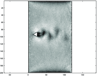
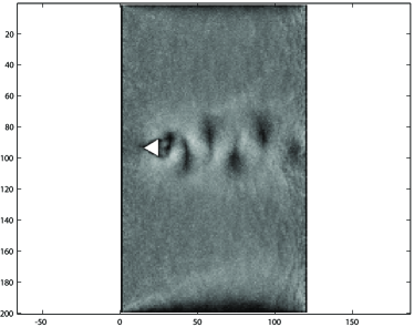
Figure 2: Wake of a triangular obstacle at source-sink ratio 0.6/0.1 for two versions of FHP. The velocity magnitude is represented by different shades of gray. White bitmap image of the triangular object has been placed by hand on top of the calculated velocity field. Left panel: FHP-II. Right panel: FHP-III.

The creation probabilities of $0.6$ and $0.1$ of the source/sink zones have been used, and a simulation of 30000 steps has been carried out on a lattice of 120x200 blocks. The absolute magnitude of the velocity displayed in 100 shades of gray (white being highest magnitude) is shown. Note that the Kármán vortex street is clearly visible in both FHP-II and FHP-III models (left and right panels of Fig. 2, respectively). However, one can also notice that FHP-III produces more pronounced vortices than FHP-II, owing to the lower viscosity and therefore a higher Reynolds number review:dHumieres_Lallemand . The lower viscosity of the FHP-III model stems from its expanded set of possible collisions. In the latter, 76 configurations participate in collisions, as opposed to merely 22 such active configurations of the FHP-II model. We refer the reader to Refs. review:dHumieres_Lallemand and thesis:wylie_1990 , where these collisions are listed explicitly. For this reason, we consider the FHP-III rule set to be more suitable for the measurement of the Strouhal number, as it produces clearer vortices with no additional computational effort. Thus, the FHP-III model has been used for the simulations of the vortex flow meter.

III.3 Vortex flow meter

The main part of our investigation consists of measurements of the vortex shedding frequency dependence on the flow rate in the two-dimensional simulation of a vortex flow meter article:reik_et_al_2010 using the FHP-III rule set. The results have then been used to determine the Reynolds-Strouhal number dependence.

The two-dimensional model of a vortex flow meter consists of a flow in a channel with impermeable walls and a trapezoid-shaped obstacle that constitutes the vortex shedding device. We have considered two cases differing in the obstacle to channel size ratio, i.e., the ratio between the length $L$ of the longer base of the vortex shedding device and the width $D$ of the channel. All simulations used a geometrically similar vortex shedding device with the length of the shorter base and the height of the trapezoid proportional to $L$ and equal to $0.225\,L$ and $1.1\,L$, respectively. The geometry is depicted in Fig. 3. Here, the general flow direction is indicated by the gray arrow.

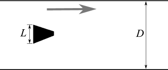
Figure 3: Geometry of the vortex flow meter simulation.

We have investigated a relatively small vortex shedding device with obstacle to channel ratio $L/D=0.055$ and a large vortex shedding device with $L/D=0.27$. This particular choice of the two ratios has been made for two reasons. First, these choices address the two opposite physical limits: (i) the transparent situation where the vortices are shed far from the walls of the pipe ($L/D=0.055\ll 1)$, and also (ii) the less intuitive case where the boundary effects should play an important role ($L/D=0.27\sim 1$). Moreover, the number $0.27$ has been read off the geometry of the industrial vortex flow meter investigated in Ref. article:reik_et_al_2010 , in order to make a contact with the results presented there. In both cases the $y$ component of the velocity $v_{y}$ (velocity in the direction perpendicular to the channel flow direction) has been measured 5 cells downstream from the shorter base of the trapezoid that constitutes our vortex shedding device. This corresponds to the lattice-gas implementation of hot-wire anemometry. Vortex shedding has produced sine-shaped variation in $v_{y}$. An example piece of raw data that has been measured in the simulation is depicted in Fig. 4 together with the sine function fit from which the vortex shedding frequency is determined.

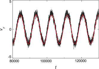
Figure 4: Dynamics (in time steps) of the velocity perpendicular to the channel direction used for determination of the wake oscillation frequency. Here the case of the small vortex shedding device at small flow velocity $u=0.267$ ($Re=156$) is shown. The black line represents the output and the red line represents the sine fit for the frequency $0.0001$.

The Reynolds number $Re$ and the Strouhal number $St$ have been calculated from the measured flow velocity $u$ and the vortex shedding frequency $f$ using (3) and (4), respectively. The velocity $u$ has been tuned by changing the source/sink ratio of the particle-absorbing/producing zones described in Subsection III.1. It has been measured by averaging across the channel upstream from the obstacle.

III.3.1 Small vortex shedding device

For the simulation with a small vortex shedding device where $L/D=0.055$, a system of $120\times 200$ cells (each cell, as before, being a $16\times 16$ block of lattice nodes) has been used. The measured vortex shedding frequency $f$ dependence on the flow velocity $u$ and the computed $St(Re)$ dependence are shown in Fig. 5.

An approximate linear dependence of $f$ on the velocity $u$ has been observed:

$$f=-(1\pm 0.1)\cdot 10^{-4}+(7.8\pm 0.3)\cdot 10^{-4}\cdot u$$ (5)

The uncertainties here are the errors in the least-squares linear fit of the data.

However, one notices that the linear dependence is not ideal. First of all, it would give a non-zero frequency $f$ for $u=0$. Secondly, one can see a nonlinear trend in the data (see left panel of Fig. 5) which suggests that $St$ is not constant. The latter fact is clearly visible when looking at the $St(Re)$ dependence computed from the data (see right panel of Fig. 5).

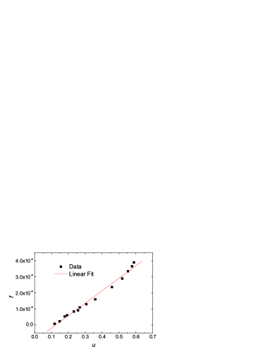
Figure 5: Measurements for the small vortex shedding device ($L/D=0.055$, see Fig. 3). Left panel: vortex shedding frequency dependence on flow velocity with linear fit (solid red line). Right panel: Strouhal-Reynolds number dependence.

III.3.2 Large vortex shedding device

The authors of Ref. article:reik_et_al_2010 have observed the decrease in Strouhal number $St$ with increasing Reynolds number $Re$ for $Re<4800$ and suggested that the reason for this dependence might be related to the formation of horseshoe vortices along the channel walls and the three-dimensional turbulent flow.

Both of these effects are specific for a three-dimensional geometry, and therefore do not exist in our flat model. It is thus useful to study if the previously reported trend in the $St(Re)$ dependence survives given the decreased dimensionality of the system.

Results for the simulation of a large vortex shedding device with $L/D=0.27$ are shown in Fig. 6. Here, a system of $240\times 100$ cells has been used. The ratio $L/D=0.27$ has been chosen to be the same as has been used in Ref. article:reik_et_al_2010 thus allowing a direct comparison of our results with the ones presented in Ref. article:reik_et_al_2010 for the three-dimensional case. Due to the interaction between the vortex street and the channel walls, a very noisy signal has been obtained. The dependence of the frequency $f$ on $u$ might still be considered as slightly increasing (left panel of Fig. 6):

$$f=-(0.1\pm 0.1)\cdot 10^{-4}+(1.2\pm 0.5)\cdot 10^{-4}\cdot u\,\,,$$ (6)

but no clear trend in the dependence of $St$ on $Re$ is apparent (right panel of Fig. 6).

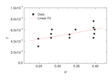
Figure 6: Measurements for the large vortex shedding device ($L/D=0.27$, see Fig. 3). Left panel: vortex shedding frequency dependence on flow velocity with linear fit (solid red line). Right panel: Strouhal-Reynolds number dependence.

IV Summary and conclusions

In summary, this paper presents three main results from a series of two-dimensional hydrodynamic simulations using the FHP lattice gas models.

First, the Poiseuille profile for the laminar flow confined in a channel has been demonstrated using the source/sink method. It has also been shown that the so-called fan approach for induction of the flow results in a different, namely, rectangular, velocity profile (Fig. 1).

Moreover, the vortex shedding from a triangular object in the flow has been demonstrated in FHP-II and FHP-III models, exhibiting higher viscosity in the FHP-II model (Fig. 2). Therefore, the FHP-III model has been used for further simulations.

The main part of this paper has been the simulation of the vortex shedding from a blunt trapezoid-shaped obstacle (Fig. 3) in a confined flow. This configuration is a model for the vortex flow meter described in Ref. article:reik_et_al_2010 . The Strouhal-Reynolds number dependence was investigated in two different obstacle-channel size ratios.

As already noticed in classical works (see, e.g., Ref. article:ssb88prl ), statistical fluctuations play a prominent role in lattice gas automaton simulations in general, and in turbulence-related problems in particular. Having this limitation of our method in mind, we have performed the simulation multiple times in order to investigate run-to-run noise. We have discovered that the differences between runs are appreciable only for the large vortex shedding device case. Hence, we only show the results of different runs for that case (see Fig. 6). However, in order to fully ascertain that the results are not dependent on the statistical fluctuations, one should turn to more sophisticated methods (see Refs. article:mz88prl ; article:hsb89epl ).

Linear dependence (see Eq. (5)) of the vortex shedding frequency on the flow velocity and increasing Strouhal number with increasing Reynolds number has been demonstrated (Fig. 5) for the small vortex shedding device.

For the large vortex shedding device, where the vortex street is obstructed by the channel walls, only a weak dependence of the vortex shedding frequency on the flow velocity can be observed (see Eq. (6), Fig. 6) and no significant Strouhal-Reynolds dependence has been found in contrast to the experimental data and hydrodynamic simulations given in Ref. article:reik_et_al_2010 . Therefore, our two-dimensional results support the hypothesis presented in Ref. article:reik_et_al_2010 , namely, that flow structures particular to the three-dimensional geometry are responsible for the strong $St(Re)$ dependence.

In future work, it would be interesting to study the transition from two dimensions to three dimensions, as the onset of the strong $St(Re)$ dependence is expected to occur when the extent of the smallest dimension of the system surpasses the length scale characteristic to the flow. Therefore, in pipes smaller than the size of the horseshoe vortex (given a certain flow velocity), vortex flow meters operate in the accurate linear regime, whereas when the diameter of the pipe is sufficiently large, the accuracy of the said flow meters should decrease. These investigations might lead to a better understanding of the reliable-operation bounds of the industrial vortex flow meters.

V Acknowledgements

It is our pleasure to thank G. T. Barkema for introducing us to the FHP models. We also thank J. Bučinskas for his spirited encouragement to publish our results. J. A. was supported by European Union’s Horizon 2020 research and innovation programme under the Marie Skłodowska-Curie grant agreement No 706839 (SPINSOCS).

References

- (1) L. P. Pitaevskii and S. Stringari, Bose-Einstein Condensation and Superfluidity (Oxford Univ. Press., 2016)
- (2) P. A. Irwin, Vortices and tall buildings: A recipe for resonance, Phys. Today 63, 68-69 (2010)
- (3) C. L. Fefferman, Existence and smoothness of the Navier Stokes equation, http://www.claymath.org/sites/default/files/navierstokes.pdf
- (4) T. K. Sengupta, Instabilities of Flows: with and without heat transfer and chemical reaction (Springer, 2010)
- (5) A. Mallock, On the resistance of air, Proc. Royal Soc. A79, 262–265 (1907)
- (6) H. Bénard, Formation périodique de centres de giration à l’arrière d’un obstacle en mouvement, C. R. Acad. Sci., 147, 839-842 (1908)
- (7) T. von Kármán, Aerodynamics (McGraw-Hill, 1954)
- (8) W. Boyes (Ed.), Instrumentation Reference Book, 4th Edition (Butterworth-Heinemann, 2009)
- (9) M. Reik, R. Höcker, C. Bruzesse, M. Hollmach, O. Koudal, T. Schenkel, H. Oertel, Flow rate measurement in a pipe flow by vortex shedding, Forsch. Ingenieurwes. 74, 77-86 (2010)
- (10) T. Bohr, M. H. Jensen, G. Paladin and A. Vulpiani, Dynamical Systems Approach to Turbulence (Cambridge Univ. Press, 1998)
- (11) H. L. Swinney (Ed.) and J. P. Gollub (Ed.), Hydrodynamic Instabilities and the Transition to Turbulence (Springer Verlag, Berlin, 1981)
- (12) A. S. Monin and A. M. Yaglom, Statistical Fluid Mechanics, Vol. 1 (MIT Press, Cambridge, 1971)
- (13) A. S. Monin and A. M. Yaglom, Statistical Fluid Mechanics, Vol. 2 (MIT Press, Cambridge, 1971)
- (14) A. N. Kolmogorov, The local structure of turbulence in incompressible viscous fluid for very large Reynolds numbers, C. R. Acad. Sci. USSR, 30, 301-305 (1941)
- (15) A. N. Kolmogorov, A refinement of previous hypotheses concerning the local structure of turbulence in incompressible viscous fluid for very large Reynolds numbers, J. Fluid Mech. 13, 82-85 (1962)
- (16) S. Wolfram, Cellular automaton fluids 1: Basic theory, J. Stat. Phys. 45 (3-4), 471-526 (1986)
- (17) B. J. N. Wylie, Application of Two-Dimensional Cellular Automaton Lattice-Gas Models to the Simulation of Hydrodynamics, PhD thesis, University of Edinburgh (1990)
- (18) J.-P. Rivet and J. P. Boon, Lattice Gas Hydrodynamics (Cambridge Univ. Press, 2001)
- (19) U. Frish, B. Hasslacher, and Y. Pomeau, Lattice-gas automata for the Navier-Stokes equation, Phys. Rev. Lett. 56, 1505 (1986)
- (20) J. Hickey, I. L’Heureux, Classical nucleation theory with a radius-dependent surface tension: A two-dimensional lattice-gas automata model, Phys. Rev. E 87, 022406 (2013)
- (21) X. Gao, C. Narteau, O. Rozier, S. C. Du Pont, Phase diagrams of dune shape and orientation depending on sand availability, Scientific reports, 5 (2015)
- (22) A. Klales, D. Cianci, Z. Needell, D. A. Meyer, P. J. Love, Lattice gas simulations of dynamical geometry in two dimensions, Phys. Rev. E 82, 046705 (2010)
- (23) S. Succi, The Lattice Boltzmann Equation for Fluid Dynamics and Beyond (Oxford Univ. Press, 2001)
- (24) L. D. Landau and E. M. Lifshitz, Course of Theoretical Physics Vol. 6. Fluid Mechanics, 2nd. English edition Elsevier Ltd. (1987)
- (25) A. Roshko, On the Development of Turbulent Wakes from Vortex Streets, NACA Report 1191 (1954)
- (26) D. d’Humieres and P. Lallemand, Numerical simulations of hydrodynamics with lattice gas automata in two dimensions, Complex Systems 1, 599-632 (1987)
- (27) S. Succi, P. Santangelo, and R. Benzi, High-Resolution Lattice-Gas Simulation of Two-Dimensional Turbulence, Phys. Rev. Lett. 60, 2738 (1988)
- (28) G. R. McNamara and G. Zanetti, Use of the Boltzmann Equation to Simulate Lattice-Gas Automata, Phys. Rev. Lett. 61, 2332 (1988)
- (29) F. J. Higuera, S. Succi and R. Benzi, Lattice Gas Dynamics with Enhanced Collisions, EPL 9, 345 (1989)