Improved method for generating exchange-correlation potentials from electronic wave functions

Abstract

Ryabinkin, Kohut, and Staroverov (RKS) [Phys. Rev. Lett. 115, 083001 (2015)] devised an iterative method for reducing many-electron wave functions to Kohn–Sham exchange-correlation potentials, $v_{\text{XC}}(\mathbf{r})$. For a given type of wave function, the RKS method is exact (Kohn–Sham-compliant) in the basis-set limit; in a finite basis set, it produces an approximation to the corresponding basis-set-limit $v_{\text{XC}}(\mathbf{r})$. The original RKS procedure works very well for large basis sets but sometimes fails for commonly used (small and medium) sets. We derive a modification of the method’s working equation that makes the RKS procedure robust for all Gaussian basis sets and increases the accuracy of the resulting exchange-correlation potentials with respect to the basis-set limit.

I Introduction

Recently, the present authors and their co-workersRyabinkin et al. (2015); Cuevas-Saavedra et al. (2015); Cuevas-Saavedra and Staroverov (2016); Kohut et al. (2016a); Ryabinkin et al. (2016) developed a method for constructing Kohn–Sham (KS) exchange-correlation potentials, $v_{\text{XC}}(\mathbf{r})$, from electronic wave functions for nondegenerate ground states that are pure-state $v$-representable.Levy (1982); Englisch and Englisch (1983) In this method, $v_{\text{XC}}(\mathbf{r})$ is generated by iterating an analytic expression that relates this potential to the interacting two-electron reduced density matrix (2-RDM) of the system. Refs. 1 and 2 describe two implementations of our technique based on slightly different but equivalent expressions for $v_{\text{XC}}(\mathbf{r})$, Ref. 3 presents a general approach for deriving such expressions, whereas Refs. 4 and 5 elaborate on the implications. Since the two published variantsRyabinkin et al. (2015); Cuevas-Saavedra et al. (2015) of our method are interchangeable, we will refer to them collectively as the Ryabinkin–Kohut–Staroverov (RKS) procedure, after the authors of Ref. 1. In the special case of Hartree–Fock (HF) wave functions, the RKS procedure reduces to the method of Refs.8 and 9.

The RKS method is not a KS inversion technique, that is, it does not focus on finding the KS potential that reproduces a given ab initio electron density $\rho^{\text{WF}}(\mathbf{r})$. The KS inversion problem is ill-conditionedSavin et al. (2003) and its solution is not unique when the KS equations are solved in a finite one-electron basis set.Harriman (1983); Görling and Ernzerhof (1995); Staroverov et al. (2006); Pino et al. (2009) The objective of the RKS method is to approximate the basis-set-limit $v_{\text{XC}}(\mathbf{r})$ of the system when both wave-function and KS calculations are done using a finite basis set. RKS potentials are obtained from the 2-RDM via an analytic expression for $v_{\text{XC}}(\mathbf{r})$ that is exact in a complete (infinite) basis set but not in a finite one. As a consequence, they are unambiguous and uniform, but the density $\rho^{\text{KS}}(\mathbf{r})$ generated by an RKS potential is exactly equal to $\rho^{\text{WF}}(\mathbf{r})$ only in the basis-set limit. This is to be contrasted with KS inversion techniques,Görling (1992); Wang and Parr (1993); Zhao et al. (1994); van Leeuwen and Baerends (1994); Schipper et al. (1997); Peirs et al. (2003); Wu and Yang (2003); Ryabinkin and Staroverov (2012); Hollins et al. (2017) where the requirement that $\rho^{\text{KS}}(\mathbf{r})$ match $\rho^{\text{WF}}(\mathbf{r})$ in any basis set can result in potentials that oscillate, diverge, and look nothing like the $v_{\text{XC}}(\mathbf{r})$ of the basis-set limit $\rho^{\text{WF}}(\mathbf{r})$ for the same system.Schipper et al. (1997); Mura et al. (1997) Thus, KS inversion and RKS methods pose different questions and give different answers in finite basis sets.

In our experience, the RKS procedure works best for large uncontracted basis sets such as the universal Gaussian basis set (UGBS).de Castro and Jorge (1998) For general-purpose basis sets such as cc-pVXZ,Dunning, Jr. (1989) cc-pCVXZ,Woon and Dunning, Jr. (1995) and 6-311G*, it often works well, but sometimes produces deformed potentials or even fails to converge (see examples below). Here we propose a modification to the RKS method that eliminates all such problems, increases the uniformity of potentials obtained in various Gaussian basis sets, and substantially improves the accuracy of potentials generated in small basis sets with respect to the basis-set limit.

II RKS method and its modification

The exact expression for $v_{\text{XC}}$ that lies at the heart of the RKS method was obtainedRyabinkin et al. (2015); Cuevas-Saavedra et al. (2015) by combining two local energy balance equations derived within the KS and ab initio wave-function formalisms for a given $N$-electron system. These two equations contain the molecular electrostatic potential but differ in all other terms. The fact that both equations describe the same system is expressed by the condition

$$\rho^{\text{KS}}(\mathbf{r})=\rho^{\text{WF}}(\mathbf{r}).$$ (1)

When one local energy balance equation is subtracted from the other, the electrostatic potential drops out and we obtain the following intermediate result:

$$v_{\text{XC}}=v_{\text{XC}}^{\text{hole}}+\bar{\epsilon}^{\text{KS}}-\bar{\epsilon}^{\text{WF}}+\frac{\tau_{L}^{\text{WF}}}{\rho^{\text{WF}}}-\frac{\tau_{L}^{\text{KS}}}{\rho^{\text{KS}}},$$ (2)

where each quantity is a function of $\mathbf{r}$. Here

$$v_{\text{XC}}^{\text{hole}}(\mathbf{r})=\int\frac{\rho_{\text{XC}}(\mathbf{r},\mathbf{r}_{2})}{|\mathbf{r}-\mathbf{r}_{2}|}\,d\mathbf{r}_{2}$$ (3)

is the potential of the exchange-correlation hole chargeParr and Yang (1989) derived from the interacting 2-RDM,

$$\bar{\epsilon}^{\text{KS}}=\frac{1}{\rho^{\text{KS}}}\sum_{i=1}^{N}\epsilon_{i}|\phi_{i}|^{2}$$ (4)

is the average local KS orbital energy, in which $\phi_{i}$ are the spatial parts of KS spin-orbitals, $\epsilon_{i}$ are their eigenvalues, and

$$\rho^{\text{KS}}=\sum_{i=1}^{N}|\phi_{i}|^{2}.$$ (5)

The next quantity, defined by

$$\bar{\epsilon}^{\text{WF}}=\frac{1}{\rho^{\text{WF}}}\sum_{j}\lambda_{j}|f_{j}|^{2},$$ (6)

is the ab initio average local electron energy,Ryabinkin and Staroverov (2014); Kohut et al. (2016b) in which $f_{j}$ are the eigenfunctions of the generalized Fock operator, $\lambda_{j}$ are their eigenvalues, and $\rho^{\text{WF}}$ is the ab initio electron density. The summation in Eq. (6) extends over all eigenfunctions $f_{j}$ whose number is equal to the number of one-electron basis-set functions. We choose to write the ab initio electron density as

$$\rho^{\text{WF}}=\sum_{j}n_{j}|\chi_{j}|^{2},$$ (7)

where $\chi_{j}$ are the natural orbitals and $n_{j}$ are their occupation numbers. The remaining quantities are

$$\tau_{L}^{\text{WF}}=-\frac{1}{2}\Re\left[\sum_{j}n_{j}\chi_{j}^{*}\nabla^{2}\chi_{j}\right],$$ (8)

the Laplacian form of the interacting (ab initio) kinetic-energy density expressed through natural orbitals, and

$$\tau_{L}^{\text{KS}}=-\frac{1}{2}\Re\left[\sum_{i=1}^{N}\phi_{i}^{*}\nabla^{2}\phi_{i}\right],$$ (9)

the Laplacian form of the noninteracting (KS) kinetic-energy density. Note that Eq. (2) is one of an entire class of exact expressions for $v_{\text{XC}}$.Cuevas-Saavedra and Staroverov (2016); Buijse et al. (1989); Baerends and Gritsenko (1997); Chong et al. (2002)

For reasons discussed below, the RKS procedure uses not Eq. (2) but a different expression obtained from Eq. (2) by applying to $\tau_{L}^{\text{WF}}$ and $\tau_{L}^{\text{KS}}$ the identity

$$\tau_{L}=\tau-\frac{1}{4}\nabla^{2}\rho,$$ (10)

where $\tau$ denotes the respective positive-definite form of the kinetic-energy density. The terms $\nabla^{2}\rho^{\text{WF}}/4\rho^{\text{WF}}$ and $\nabla^{2}\rho^{\text{KS}}/4\rho^{\text{KS}}$ cancel out because of Eq. (1), and Eq. (2) becomes

$$v_{\text{XC}}=v_{\text{XC}}^{\text{hole}}+\bar{\epsilon}^{\text{KS}}-\bar{\epsilon}^{\text{WF}}+\frac{\tau^{\text{WF}}}{\rho^{\text{WF}}}-\frac{\tau^{\text{KS}}}{\rho^{\text{KS}}},$$ (11)

where

$$\tau^{\text{WF}}=\frac{1}{2}\sum_{j}n_{j}|\nabla\chi_{j}|^{2}$$ (12)

and

$$\tau^{\text{KS}}=\frac{1}{2}\sum_{i=1}^{N}|\nabla\phi_{i}|^{2}.$$ (13)

Equation (11) is the basis of the RKS method. To construct $v_{\text{XC}}$ by this technique one needs to compute all of the terms on the right-hand side of Eq. (11). The terms $v_{\text{XC}}^{\text{hole}}$, $\tau^{\text{WF}}$, and $\rho^{\text{WF}}$ are extracted from an ab initio wave function, but $\bar{\epsilon}^{\text{KS}}$ and $\tau^{\text{KS}}$ are initially unknown because they depend on $\phi_{i}$ and $\epsilon_{i}$, which in turn depend on $v_{\text{XC}}$. In Refs. Ryabinkin et al., 2015 and Cuevas-Saavedra et al., 2015, we showed that it is possible to simultaneously solve for $v_{\text{XC}}$ and the associated KS orbitals by starting with a reasonable initial guess for $\phi_{i}$ and $\epsilon_{i}$ and iterating Eq. (11) via the KS equations until the potential $v_{\text{XC}}$ becomes self-consistent. In a finite basis set, this potential is such that $\rho^{\text{KS}}\neq\rho^{\text{WF}}$ even at convergence.

Equations (2) and (11) are both exact (KS-compliant) only when all their right-hand-side ingredients are obtained in a complete basis set. This is because the two local energy balance equations leading to Eq. (2) were derived by analytically inverting the KS and generalized Fock eigenvalue problems,Ryabinkin et al. (2015); Cuevas-Saavedra et al. (2015) and analytic inversion of operator eigenvalue problems amounts to employing a complete basis set. Refs. 19, 24, and 34 demonstrate the dramatic effect of basis-set incompleteness on the inverted KS equation, whereas Refs. 5 and 30 illustrate it for the generalized Fock eigenvalue problem.

In a finite basis set, Eqs. (2) and (11) are not even equivalent because Eq. (1), which links them, does not hold from the start of iterations. Previously we found that iterations of Eq. (2) hardly ever converge, whereas iterations of Eq. (11) converge for many, but not all, standard Gaussian basis sets. We now argue that Eq. (11) works better than Eq. (2) because in Eq. (11) the difference $\nabla^{2}\rho^{\text{WF}}/4\rho^{\text{WF}}-\nabla^{2}\rho^{\text{KS}}/4\rho^{\text{KS}}$ is set to its basis-set-limit value of zero even when $\rho^{\text{KS}}\neq\rho^{\text{WF}}$, so the resulting finite-basis-set $v_{\text{XC}}$ can get closer to the basis-set-limit potential. Motivated by this idea, we propose the following improvement upon Eq. (11).

Let us assume for simplicity that all $\phi_{i}$ are real. Using the Lagrange identityMitrinović (1970) we write

$$2\rho^{\text{KS}}\tau^{\text{KS}} =\left(\sum_{i=1}^{N}\phi_{i}^{2}\right)\left(\sum_{i=1}^{N}|\nabla\phi_{i}|^{2}\right)$$ (14)

$$=\left|\sum_{i=1}^{N}\phi_{i}\nabla\phi_{i}\right|^{2}+\sum_{i<j}^{N}|\phi_{i}\nabla\phi_{j}-\phi_{j}\nabla\phi_{i}|^{2}.$$

Recognizing that $|\sum_{i=1}^{N}\phi_{i}\nabla\phi_{i}|^{2}=|\nabla\rho^{\text{KS}}|^{2}/4$ and dividing Eq. (14) through by $2\rho^{\text{KS}}$ we have (cf. Ref. 36)

$$\tau^{\text{KS}}=\tau_{W}^{\text{KS}}+\tau_{P}^{\text{KS}},$$ (15)

where $\tau_{W}^{\text{KS}}=|\nabla\rho^{\text{KS}}|^{2}/8\rho^{\text{KS}}$ is the von Weizsäcker noninteracting kinetic-energy density and

$$\tau_{P}^{\text{KS}}=\frac{1}{2\rho^{\text{KS}}}\sum_{i<j}^{N}|\phi_{i}\nabla\phi_{j}-\phi_{j}\nabla\phi_{i}|^{2}$$ (16)

is a quantity which we call the Pauli kinetic-energy density (the name is motivated by Ref.37). Similarly, assuming real natural orbitals and applying the Lagrange identity to the product $2\rho^{\text{WF}}\tau^{\text{WF}}$ we obtain

$$\tau^{\text{WF}}=\tau_{W}^{\text{WF}}+\tau_{P}^{\text{WF}},$$ (17)

where $\tau_{W}^{\text{WF}}=|\nabla\rho^{\text{WF}}|^{2}/8\rho^{\text{WF}}$ and

$$\tau_{P}^{\text{WF}}=\frac{1}{2\rho^{\text{WF}}}\sum_{i<j}n_{i}n_{j}|\chi_{i}\nabla\chi_{j}-\chi_{j}\nabla\chi_{i}|^{2}.$$ (18)

Next we substitute Eqs. (15) and (17) into Eq. (11). In view of Eq. (1), the terms $\tau_{W}^{\text{KS}}/\rho^{\text{KS}}$ and $\tau_{W}^{\text{WF}}/\rho^{\text{WF}}$ cancel out and we arrive at the following new expression,

$$v_{\text{XC}}=v_{\text{XC}}^{\text{hole}}+\bar{\epsilon}^{\text{KS}}-\bar{\epsilon}^{\text{WF}}+\frac{\tau_{P}^{\text{WF}}}{\rho^{\text{WF}}}-\frac{\tau_{P}^{\text{KS}}}{\rho^{\text{KS}}},$$ (19)

which is the main result of this work. Just like Eqs. (2) and (11), Eq. (19) is KS-compliant only in the basis-set-limit. In a finite basis set, it should give a better approximation to the basis-set-limit $v_{\text{XC}}$ than Eq. (11) because it sets the quantity $\tau_{W}^{\text{WF}}/\rho^{\text{WF}}-\tau_{W}^{\text{KS}}/\rho^{\text{KS}}$ to its basis-set-limit value of zero even when $\rho^{\text{KS}}\neq\rho^{\text{WF}}$. We will refer to the variant of our method using Eq. (19) as the modified RKS (mRKS) procedure.

The mRKS procedure is exactly the same as the original RKS methodRyabinkin et al. (2015); Cuevas-Saavedra et al. (2015); Kohut et al. (2016a) except that the former uses Eq. (19) in place of Eq. (11). Therefore, we will not describe the mRKS algorithm in detail here but only emphasize the following important points. The equality $\rho^{\text{KS}}=\rho^{\text{WF}}$ plays a key role in the derivation of Eqs. (11) and (19), but it is not imposed when these equations are solved by iteration. Thus, there is no such thing as a “target density” in the RKS and mRKS methods, and the extent to which $\rho^{\text{KS}}$ deviates from $\rho^{\text{WF}}$ at convergence is controlled implicitly through the choice of one-electron basis set. For internal consistency, the RKS and mRKS procedures use the same one-electron basis set to generate the ab initio wave function and to solve the KS equations in the iterative part of the algorithm. The Hartree (Coulomb) contribution to the KS Hamiltonian matrix is always computed using $\rho^{\text{KS}}$ (not $\rho^{\text{WF}}$); we do it analytically in terms of Gaussian basis functions. Matrix elements of $v_{\text{XC}}$ are evaluated using saturated Gauss–Legendre–Lebedev numerical integration grids. We consider $v_{\text{XC}}$ converged when the difference between two consecutive KS density matrices drops below 10^-10 in the root-mean-square sense. Both the original and modified RKS procedures require direct inversion of the iterative subspacePulay (1982) to converge the potential in self-consistent-field (SCF) iterations; the mRKS procedure typically takes one or two dozen iterations, RKS up to a few dozen. The converged $v_{\text{XC}}$ is independent of the initial guess; KS orbitals and orbital energies from any standard density-functional approximation are adequate as a starting point for systems with a single-reference character. For this work, we re-implemented the RKS and mRKS methods by modifying the SCF and multiconfigurational SCF links of a more recent version of the gaussian 09 program.G (09)

III Comparison of the original and modified RKS methods

To demonstrate the practical advantages of Eq. (19) over Eq. (11) we compared exchange-correlated potentials generated by the mRKS and RKS methods from various atomic and molecular ab initio wave functions. The wave functions were of three types: HF, complete active space SCF (CASSCF), and full configuration interaction (FCI). Wave functions of each type were obtained using a series of standard Gaussian one-electron basis sets varying between minimal (STO-3G) and very large (UGBS). All basis sets were taken from the Basis Set Exchange Database.Feller (1996); Schuchardt et al. (2007)

For each wave function, we report three relevant properties: the total interacting kinetic energy

$$T=-\frac{1}{2}\sum_{j}n_{j}\langle\chi_{j}|\nabla^{2}|\chi_{j}\rangle,$$ (20)

the ab initio exchange-correlation energy

$$E_{\text{XC}}^{\text{WF}}=\frac{1}{2}\int\rho^{\text{WF}}(\mathbf{r})v_{\text{XC}}^{\text{hole}}(\mathbf{r})\,d\mathbf{r},$$ (21)

and the first ionization energy extracted from the wave function by the extended Koopmans theoremDay et al. (1974); Smith and Day (1975); Day et al. (1975); Morrell et al. (1975); Morrison and Liu (1992); Pernal and Cioslowski (2005) (EKT), $I_{\text{EKT}}$. For HF wave functions, $I_{\text{EKT}}=-\epsilon_{\text{HOMO}}^{\text{HF}}$, where $\epsilon_{\text{HOMO}}^{\text{HF}}$ is the eigenvalue of the highest-occupied molecular orbital (HOMO). For post-HF wave functions, $I_{\text{EKT}}$ was computed as the largest eigenvalue of the $\mathbf{V}^{\prime}$ matrix defined in Ref. Morrison and Liu, 1992. The EKT ionization energies are needed to fix the constant up to which the $v_{\text{XC}}$ is defined by Eqs. (11) and (19).Ryabinkin et al. (2015); Cuevas-Saavedra et al. (2015) This is done by shifting the potential vertically so that $\epsilon_{\text{HOMO}}=-I_{\text{EKT}}$.

After reducing each ab initio wave function to a self-consistent $v_{\text{XC}}(\mathbf{r})$, we evaluated the following properties: the total noninteracting kinetic energy

$$T_{s}=-\frac{1}{2}\sum_{i=1}^{N}\langle\phi_{i}|\nabla^{2}|\phi_{i}\rangle,$$ (22)

the KS exchange-correlation energy

$$E_{\text{XC}}^{\text{KS}}=E_{\text{XC}}^{\text{WF}}+T_{c},$$ (23)

where

$$T_{c}=T-T_{s},$$ (24)

and the integral

$$W=\int\left[3\rho(\mathbf{r})+\mathbf{r}\cdot\nabla\rho(\mathbf{r})\right]v_{\text{XC}}(\mathbf{r})\,d\mathbf{r},$$ (25)

whose purpose will be explained shortly. The integrals in Eqs. (20),  (21), and (22) were computed analytically, whereas $W$ was evaluated numerically.

Strictly speaking, the quality of mRKS potentials should be judged by their proximity to the basis-set-limit $v_{\text{XC}}$, but since exact exchange-correlation potentials are rarely available, we suggest to use weaker but feasible tests for basis-set completeness. The first test is the integrated density error

$$\Delta_{\rho}=\int\left|\rho^{\text{KS}}(\mathbf{r})-\rho^{\text{WF}}(\mathbf{r})\right|\,d\mathbf{r}\geq 0,$$ (26)

where $\rho^{\text{KS}}(\mathbf{r})$ is evaluated at convergence. For a given type of wave function, $\Delta_{\rho}$ is uniquely determined by the basis set used in the mRKS procedure. The premise of the test is that $\Delta_{\rho}$ tends to zero as the basis set approaches completeness, so the magnitude of $\Delta_{\rho}$ gives some indication of how close the mRKS potential is to its basis-set limit. We emphasize that $\Delta_{\rho}$ values have entirely different meanings in KS inversion and RKS-type methods. For instance, $\Delta_{\rho}\approx 0.05$ a.u. in a KS inversion procedure indicates that $v_{\text{XC}}$ is not converged, whereas in the mRKS procedure it signals that the corresponding converged $v_{\text{XC}}$ is not yet close to the basis-set-limit potential (because an insufficiently large basis set was used).

The second test is based on the fact that, for a given density functional $E_{\text{XC}}[\rho]$ and a density $\rho(\mathbf{r})$, the corresponding functional derivative $v_{\text{XC}}(\mathbf{r})=\delta E_{\text{XC}}[\rho]/\delta\rho(\mathbf{r})$ satisfies the virial relationLevy and Perdew (1985)

$$W=E_{\text{XC}}^{\text{KS}}+T_{c},$$ (27)

where $W$ is given by Eq. (25). The magnitude of the deviation

$$\Delta E_{\text{vir}}=W-E_{\text{XC}}^{\text{KS}}-T_{c}=W-E_{\text{XC}}^{\text{WF}}-2T_{c}$$ (28)

from zero may be taken as a measure of deviation of a trial potential from $\delta E_{\text{XC}}[\rho]/\delta\rho(\mathbf{r})$. As a quality control test, $|\Delta E_{\text{vir}}|$ is more discriminating than $\Delta_{\rho}$: even visually imperceptible defects of $v_{\text{XC}}(\mathbf{r})$ can result in large $\Delta E_{\text{vir}}$ values, as we showed previously for approximate exchange-only potentials.Gaiduk and Staroverov (2008); Staroverov (2008); Ryabinkin et al. (2013); Kohut et al. (2014) Note that in Refs. 8 and 9 we studied KS potentials extracted from HF wave functions as approximations to exact-exchange potentials, for which $T_{c}=0$, so we defined $\Delta E_{\text{vir}}=W-E_{\text{X}}^{\text{HF}}$ and evaluated $E_{\text{X}}^{\text{HF}}$ using the KS (not HF) orbitals. This is why the HF/UGBS values of $\Delta E_{\text{vir}}$ in this work are different from those reported in Refs.8 and 9.

Table 1: Selected characteristics of various atomic wave functions and of the exchange-correlation potentials generated from those wave functions by the RKS and mRKS methods. $\Delta_{\rho}$ values are in units of electron charge, the rest are in hartrees. The zeros not followed by decimal figures mean “exactly zero”.

				RKS			mRKS
Basis set	$T$	$E_{\text{XC}}^{\text{WF}}$	$I_{\text{EKT}}$	$T_{s}$	$\Delta E_{\text{vir}}$	$\Delta_{\rho}$	$T_{s}$	$\Delta E_{\text{vir}}$	$\Delta_{\rho}$
Be, HF SCF
STO-3G	$14.844185$	$-2.768067$	0.2540	$14.844185$	$0.003001$	$0$	$14.844185$	$0.003001$	$0$
cc-pCVDZ	$14.571730$	$-2.667161$	0.3091	SCF fails to converge			$14.583020$	$0.026191$	$0.0096$
cc-pCVTZ	$14.572722$	$-2.666932$	0.3093	$14.549079$	$-0.016873$	$0.0123$	$14.574235$	$0.003444$	$0.0112$
cc-pCVQZ	$14.572929$	$-2.666929$	0.3093	$14.582472$	$0.009668$	$0.0047$	$14.572859$	$0.001138$	$0.0043$
UGBS	$14.573022$	$-2.666914$	0.3093	$14.572575$	$0.000138$	$0.0013$	$14.572484$	$0.000045$	$0.0014$
Numerical grid	$14.573023$	$-2.666914$	0.3093				$14.572462$	$6.4\times 10^{-12}$	$2.4\times 10^{-12}$
Be, FCI
cc-pCVDZ	$14.647784$	$-2.815393$	0.3410	$14.634247$	$0.036533$	$0.0238$	$14.584365$	$0.012058$	$0.0159$
cc-pCVTZ	$14.659118$	$-2.834119$	0.3419	$14.554768$	$-0.025476$	$0.0052$	$14.586875$	$0.000927$	$0.0052$
cc-pCVQZ	$14.663862$	$-2.839342$	0.3423	$14.595868$	$0.005482$	$0.0047$	$14.591807$	$0.001910$	$0.0054$
Basis-set limit	$14.66736$	$-2.8433$	0.3426	$14.5942$			$14.5942$
Ne, (8,8)CASSCF
3-21G	$127.526022$	$-12.331354$	0.7418	$127.146953$	$-0.317862$	$0.0242$	$127.259455$	$-0.235164$	$0.0269$
6-31G	$128.368644$	$-12.299273$	0.7701	$128.074403$	$-0.057903$	$0.0343$	$128.207015$	$0.070006$	$0.0419$
6-311G	$128.643794$	$-12.310115$	0.7889	$128.368172$	$0.054083$	$0.0119$	$128.551997$	$0.152103$	$0.0100$
cc-pVDZ	$128.379168$	$-12.295050$	0.7712	$128.091704$	$-0.065663$	$0.0354$	$128.217811$	$0.073355$	$0.0429$
cc-pVTZ	$128.699598$	$-12.313278$	0.7972	SCF fails to converge			$128.319831$	$-0.440787$	$0.0154$
cc-pVQZ	$128.679046$	$-12.310777$	0.8017	$128.401283$	$-0.166744$	$0.0119$	$128.527364$	$-0.055301$	$0.0115$
cc-pV5Z	$128.681107$	$-12.308871$	0.8036	SCF fails to converge			$128.544494$	$-0.038485$	$0.0127$
cc-pV6Z	$128.680330$	$-12.308590$	0.8038	$129.471075$	$0.850616$	$0.0275$	$128.568158$	$-0.011267$	$0.0129$
cc-pCVDZ	$128.449457$	$-12.299356$	0.7719	$128.585448$	$0.305618$	$0.0337$	$128.447270$	$0.233908$	$0.0339$
cc-pCVTZ	$128.694070$	$-12.315890$	0.7978	$128.991030$	$0.391687$	$0.0110$	$128.624258$	$0.044520$	$0.0099$
cc-pCVQZ	$128.682785$	$-12.311376$	0.8019	$128.639121$	$0.054117$	$0.0079$	$128.583579$	$0.000298$	$0.0088$
cc-pCV5Z	$128.680478$	$-12.308899$	0.8036	$128.573403$	$-0.005645$	$0.0022$	$128.578853$	$-0.000630$	$0.0025$
cc-pCV6Z	$128.680103$	$-12.308582$	0.8038	$128.579759$	$0.000595$	$0.0009$	$128.579291$	$0.000100$	$0.0010$
UGBS	$128.679971$	$-12.308530$	0.8039	$128.579178$	$0.000069$	$0.0004$	$128.579203$	$0.000089$	$0.0005$
Ar, HF SCF
STO-3G	$512.489655$	$-30.273170$	0.4959	$512.489655$	$-0.925101$	$0$	$512.489655$	$-0.925101$	$0$
6-31G	$526.813061$	$-30.189268$	0.5889	$526.566956$	$-0.285033$	$0.0238$	$526.598840$	$-0.027741$	$0.0343$
6-311G	$526.800338$	$-30.186097$	0.5901	$528.020941$	$0.260067$	$0.0495$	$526.131112$	$-0.942386$	$0.0413$
cc-pVDZ	$526.799649$	$-30.189363$	0.5880	$526.499343$	$-0.366185$	$0.0259$	$526.552243$	$-0.118648$	$0.0386$
cc-pVTZ	$526.813176$	$-30.186281$	0.5901	$526.245858$	$-1.002952$	$0.0407$	$526.415203$	$-0.491103$	$0.0649$
cc-pVQZ	$526.817051$	$-30.185184$	0.5909	$526.517557$	$-0.648849$	$0.0295$	$526.548203$	$-0.222111$	$0.0439$
cc-pV5Z	$526.817410$	$-30.185018$	0.5910	$526.852022$	$-0.263872$	$0.0339$	$526.839832$	$0.081888$	$0.0510$
cc-pV6Z	$526.818234$	$-30.184971$	0.5910	$525.371226$	$-0.890411$	$0.0404$	$526.994170$	$0.400168$	$0.0326$
cc-pCVDZ	$526.783930$	$-30.189199$	0.5880	$519.362324$	$-5.498655$	$0.1435$	$526.454232$	$-0.386389$	$0.0454$
cc-pCVTZ	$526.809131$	$-30.186274$	0.5901	$533.394130$	$6.109779$	$0.0933$	$526.383224$	$-0.627448$	$0.0324$
cc-pCVQZ	$526.818135$	$-30.185181$	0.5909	$531.897248$	$4.947426$	$0.0456$	$526.796236$	$-0.013499$	$0.0163$
cc-pCV5Z	$526.817374$	$-30.185016$	0.5910	$526.701372$	$-0.107472$	$0.0085$	$526.812305$	$0.000905$	$0.0094$
cc-pCV6Z	$526.817495$	$-30.184954$	0.5910	$526.719670$	$-0.089087$	$0.0093$	$526.814256$	$0.002980$	$0.0103$
UGBS	$526.817656$	$-30.184992$	0.5910	$526.816951$	$0.004847$	$0.0060$	$526.811751$	$-0.000259$	$0.0068$
Basis-set limit	$526.817513$		0.5910

Table 1 summarizes results of RKS and mRKS calculations for HF, CASSCF, and FCI wave functions of a few atoms. The two methods produce potentials with very similar $T_{s}$ values, small $\Delta E_{\text{vir}}$, and $\Delta_{\rho}\sim 10^{-3}$ a.u. when a large basis set (e.g., UGBS) is used. This is in accord with our argument that the RKS and mRKS procedures would be equivalent in the basis-set limit. A separate grid-based implementationRya of the mRKS procedure for the HF wave function of Be gives $\Delta E_{\text{vir}}=6.4\times 10^{-12}$ $E_{\text{h}}$ and $\Delta_{\rho}=2.4\times 10^{-12}$ a.u., which explicitly shows that the method is KS-compliant in the basis-set limit.

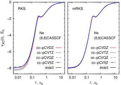
Figure 1: Exchange-correlation potentials obtained from CASSCF/cc-pCVXZ wave functions of the Ne atom using the RKS and mRKS methods. The exact $v_{\text{XC}}$ is from Ref. Filippi et al., 1996. The mRKS potentials are less sensitive to basis-set incompleteness than RKS. See Table 1 for the accompanying numerical data.

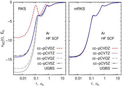
Figure 2: Exchange-correlation potentials obtained from HF/cc-pCVXZ wave functions of the Ar atom using the RKS and mRKS methods. In this particular case, RKS potentials are accurate only if computed using very large basis sets. See Table 1 for the accompanying numerical data.

For small and medium basis sets, however, the original RKS method has inconsistent performance. For instance, in the case of (8,8)CASSCF/cc-pVXZ wave functions of the Ne atom, the RKS procedure fails to converge for the cc-pVTZ and cc-pV5Z basis sets, and even though it converges for the other cc-pVXZ basis sets, the results show no clear trend with respect to basis set variations. By contrast, mRKS potentials obtained from the same wave functions produce consistent $T_{s}$ values, and $|\Delta E_{\text{vir}}|$ generally decreases with increasing basis-set size. Similar observations apply to potentials generated for other atoms. In the case of HF/cc-pCVXZ wave functions of the Ar atom, RKS potentials for basis sets smaller than cc-pCV5Z are too high or too low near the nucleus (Fig. 2) and have virial energy discrepancies of up to 6 $E_{\text{h}}$ (Table 1). At the same time, plots of mRKS potentials of the HF/cc-pCVXZ series are barely distinguishable (Fig. 2). Overall, the mRKS method performs extremely well for basis sets of any size, whereas the RKS procedure is reliable only for large basis sets.

Figures 1 and 2 highlight a common feature of all RKS and mRKS potentials: they are smooth and have no spurious oscillations that plague optimized effective potential methodsHirata et al. (2001); Staroverov et al. (2006); Görling et al. (2008); Jacob (2011); Gidopoulos and Lathiotakis (2012) and KS inversion techniques that fit potentials to Gaussian-basis-set densities.Schipper et al. (1997); Mura et al. (1997); de Silva and Wesolowski (2012); Kananenka et al. (2013); Gaiduk et al. (2013) This is because Eqs. (11) and (19) contain only terms that are well-behaved in any reasonable basis set. Note also that for a number of potentials shown in Figs. 1 and 2, $|\Delta E_{\text{vir}}^{\text{mRKS}}|\ll|\Delta E_{\text{vir}}^{\text{RKS}}|$ even though $\Delta_{\rho}^{\text{mRKS}}>\Delta_{\rho}^{\text{RKS}}$. In such cases, the mRKS potential is visually closer to the basis-set limit, which suggests that the virial energy discrepancy test is more sensitive than the density error test.

Detailed analysis of discrepancies between $\rho^{\text{KS}}(\mathbf{r})$ and $\rho^{\text{WF}}(\mathbf{r})$ for the potentials shown in Figs. 1 and 2 furnishes another demonstration that, for large basis sets, the RKS and mRKS procedures are practically equivalent and produce nearly KS-compliant potentials (Figs. 3 and 4). For small and medium basis sets, mRKS densities have much smaller deviations from $\rho^{\text{WF}}(\mathbf{r})$ near atomic nuclei than do RKS densities.

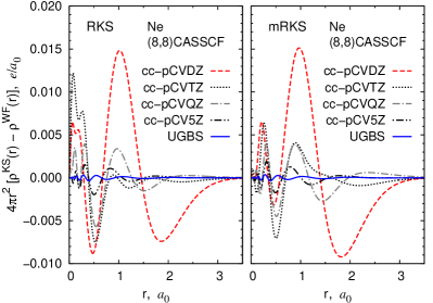
Figure 3: Discrepancies between the radial KS and ab initio densities for the exchange-correlation potentials of Fig. 1.

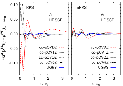
Figure 4: Discrepancies between the radial KS and ab initio densities for the exchange-correlation potentials of Fig. 2.

RKS and mRKS calculations for HF wave functions of certain systems exhibit a curious basis-set effect: the use of a minimal basis sets results in $\Delta_{\rho}=0$ (Table 1, HF/STO-3G for Be and Ar). This occurs when there are no virtual HF orbitals or when no virtual orbital has the symmetry of any occupied orbital; then the (m)RKS procedure yields occupied KS orbitals that are unitarily transformed occupied HF orbitals, which implies $\rho^{\text{KS}}=\rho^{\text{HF}}$. However, in such cases $\Delta E_{\text{vir}}\neq 0$, meaning that the (m)RKS potential is not truly KS-compliant.

The mRKS method also works well for molecules. To demonstrate this, we generated exchange-correlation potentials from HF and full-valence CASSCF wave functions of the HCN molecule using various standard Gaussian basis sets. Here the original RKS method again failed to converge for some basis sets, whereas the mRKS procedure converged without difficulty in all cases (Table 2). As in the examples involving atoms, the converged RKS and mRKS potentials for HCN are similar and become practically identical for large basis sets such as cc-pCV5Z. Moreover, mRKS potentials for HCN obtained with increasingly large basis sets of the cc-pCVXZ ($\mbox{X}=\mbox{D},\mbox{T},\mbox{Q},\mbox{5}$) series are virtually indistinguishable by eye (Fig. 5), which shows that it is not necessary to use large basis sets in the mRKS method to obtain eminently reasonable potentials.

Table 2: Selected characteristics of HF and full-valence CASSCF functions of the HCN molecule at the equilibrium geometry ($r_{\text{HC}}=2.013a_{0}$, $r_{\text{CN}}=2.179a_{0}$) and of the exchange-correlation potentials generated from those wave functions by the RKS and mRKS methods. $\Delta_{\rho}$ values are in units of electron charge, the rest are in hartrees.

				RKS			mRKS
Basis set	$T$	$E_{\text{XC}}^{\text{WF}}$	$I_{\text{EKT}}$	$T_{s}$	$\Delta E_{\text{vir}}$	$\Delta_{\rho}$	$T_{s}$	$\Delta E_{\text{vir}}$	$\Delta_{\rho}$
HCN, HF SCF
6-31G*	$92.550286$	$-12.041974$	0.4906	$91.711955$	$-0.947891$	0.0859	$92.307987$	$-0.484915$	0.0702
6-311G**	$92.742692$	$-12.046387$	0.4950	SCF fails to converge			$92.734609$	$-0.005396$	0.0578
cc-pCVDZ	$92.648587$	$-12.046478$	0.4925	SCF fails to converge			$92.716824$	$0.105823$	0.0501
cc-pCVTZ	$92.724093$	$-12.048439$	0.4957	$92.759771$	$0.035200$	0.0243	$92.756065$	$0.053961$	0.0266
cc-pCVQZ	$92.728654$	$-12.047784$	0.4967	$92.794723$	$0.064605$	0.0122	$92.729610$	$0.008136$	0.0128
cc-pCV5Z	$92.729614$	$-12.047401$	0.4970	$92.718948$	$-0.010551$	0.0066	$92.727317$	$0.003108$	0.0072
aug-cc-pCVDZ	$92.618227$	$-12.034752$	0.4972	SCF fails to converge			$92.685523$	$0.103478$	0.0493
aug-cc-pCVTZ	$92.714623$	$-12.045619$	0.4969	$92.734796$	$0.019105$	0.0218	$92.743953$	$0.048228$	0.0222
aug-cc-pCVQZ	$92.726488$	$-12.047072$	0.4970	$92.790808$	$0.061456$	0.0113	$92.727416$	$0.007485$	0.0114
aug-cc-pCV5Z	$92.729420$	$-12.047335$	0.4970	SCF fails to converge			$92.726972$	$0.002954$	0.0062
HCN, (10,9)CASSCF
6-31G*	$92.942118$	$-12.312273$	0.5224	$92.232843$	$-0.701261$	0.0525	$92.573544$	$-0.435253$	0.0521
6-311G**	$93.093351$	$-12.307472$	0.5192	SCF fails to converge			$92.974910$	$0.039466$	0.0457
cc-pVDZ	$93.010939$	$-12.305411$	0.5168	$92.767530$	$-0.112071$	0.0531	$92.777863$	$-0.071566$	0.0578
cc-pVTZ	$93.062905$	$-12.306247$	0.5208	$94.792641$	$1.309037$	0.1795	$92.800576$	$-0.263447$	0.0452
cc-pVQZ	$93.077491$	$-12.307166$	0.5213	SCF fails to converge			$92.962057$	$-0.006661$	0.0347
cc-pV5Z	$93.079200$	$-12.306930$	0.5214	$93.972821$	$0.903219$	0.0656	$92.987779$	$0.017106$	0.0260
cc-pCVDZ	$92.988167$	$-12.305592$	0.5179	SCF fails to converge			$92.886229$	$0.059178$	0.0419
cc-pCVTZ	$93.077684$	$-12.307350$	0.5212	$93.027971$	$0.050491$	0.0208	$93.010944$	$0.044703$	0.0239
cc-pCVQZ	$93.079442$	$-12.307294$	0.5214	$93.046686$	$0.056174$	0.0122	$92.988799$	$0.005245$	0.0132
cc-pCV5Z	$93.080131$	$-12.307031$	0.5214	$92.979526$	$-0.006572$	0.0061	$92.986814$	$0.002105$	0.0070

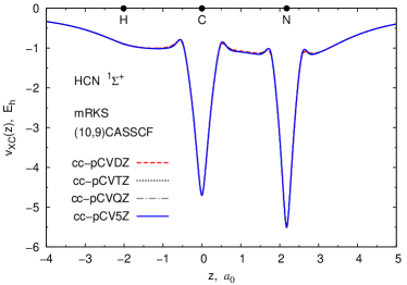
Figure 5: Exchange-correlation potentials obtained by the mRKS method from full-valence CASSCF wave functions of the HCN molecule. See Table 2 for the accompanying numerical data.

An example of an mRKS exchange-correlation potential for a polyatomic molecule (tetrafluoroethylene) is shown in Fig. 6. RKS-type potentials generated from HF wave functions are known to be excellent approximations to exchange-only optimized effective potentials.Ryabinkin et al. (2013); Kohut et al. (2014) The message of this figure is that molecular exchange-correlation potentials of high quality can be effortlessly generated by the mRKS method.

Figure 6: Exchange-correlation potential of CF₂=CF₂ obtained by the mRKS method from the HF/6-311G* wave function for the HF/6-311G* geometry. The plot shows $v_{\text{XC}}$ in the molecular plane. The $z$ axis is along the C=C bond.

IV Conclusion

We have derived Eq. (19) and showed that it works considerably better than its predecessor, Eq. (11), for the purpose of generating exchange-correlation potentials from ab initio wave functions in Gaussian basis sets. Equation (11) is in turn more useful than Eq. (2).

The transition from Eq. (2) to Eq. (11) and then to Eq. (19) is based on the relations

$$\tau_{L}=-\frac{1}{4}\nabla^{2}\rho+\tau=-\frac{1}{4}\nabla^{2}\rho+\tau_{W}+\tau_{P}$$ (29)

for each of the interacting and noninteracting systems. For $\rho^{\text{KS}}=\rho^{\text{WF}}$, these relations imply that

$$\frac{\tau_{L}^{\text{WF}}}{\rho^{\text{WF}}}-\frac{\tau_{L}^{\text{KS}}}{\rho^{\text{KS}}}=\frac{\tau^{\text{WF}}}{\rho^{\text{WF}}}-\frac{\tau^{\text{KS}}}{\rho^{\text{KS}}}=\frac{\tau_{P}^{\text{WF}}}{\rho^{\text{WF}}}-\frac{\tau_{P}^{\text{KS}}}{\rho^{\text{KS}}}.$$ (30)

Equation (29) is always true, whereas Eq. (30) holds only when $\rho^{\text{KS}}=\rho^{\text{WF}}$, which in our method happens at convergence in a complete (infinite) basis set and for minimal-basis-set HF wave functions of certain systems. This means that RKS-type iterations by Eqs. (2), (11), and (19) are generally not equivalent and should result in different potentials.

In calculations using standard Gaussian basis sets, Eq. (2) almost never converges, Eq. (11) converges for some but not all basis sets, while Eq. (19) always converges in our experience, at least for systems with a single-reference character. The RKS and mRKS methods are essentially equivalent in a nearly complete basis set, but the mRKS method is much more accurate and robust in commonly used basis sets, making it possible to routinely generate exchange-correlation potentials for atoms and molecules at any level of ab initio theory. Therefore, we recommend the mRKS procedure as a permanent replacement for the original RKS method.

The extensive numerical evidence presented in this work shows that mRKS potentials generated using incomplete (finite) basis sets are excellent approximations to the basis-set-limit $v_{\text{XC}}$ for a particular type of wave function (HF, CASSCF, FCI, etc.) The mRKS technique can also be used for construction of exchange-correlation potentials of adiabatic time-dependent density-functional theory.Lein and Kümmel (2005); Thiele et al. (2008); Elliott and Maitra (2012) Extensions of the mRKS method to spin-polarized post-HF wave functions and to systems that are not pure-state $v$-representable remain the subject of future work.