A novel quantum dynamical approach in electron microscopy
combining wave-packet propagation with Bohmian trajectories

Abstract

The numerical analysis of the diffraction features rendered by transmission electron microscopy (TEM) typically relies either on classical approximations (Monte Carlo simulations) or quantum paraxial tomography (the multislice method and any of its variants). Although numerically advantageous (relatively simple implementations and low computational costs), they involve important approximations and thus their range of applicability is limited. To overcome such limitations, an alternative, more general approach is proposed, based on an optimal combination of wave-packet propagation with the on-the-fly computation of associated Bohmian trajectories. For the sake of clarity, but without loss of generality, the approach is used to analyze the diffraction of an electron beam by a thin aluminum slab as a function of three different incidence (work) conditions which are of interest in electron microscopy: the probe width, the tilting angle, and the beam energy. Specifically, it is shown that, because there is a dependence on particular thresholds of the beam energy, this approach provides a clear description of the diffraction process at any energy, revealing at the same time any diversion of the beam inside the material towards directions that cannot be accounted for by other conventional methods, which is of much interest when dealing with relatively low energies and/or relatively large tilting angles.

I Introduction

Characterization through electron microscopy (EM) is an important aspect in materials development. Microscopic features and crystallographic information can be elucidated from high resolution and electron diffraction imaging Williams and Carter (2009). While much information can be obtained from diffraction imaging, data analysis is complex and must be coupled with simulations in order to be properly utilized. Currently, two algorithms are used to simulate selected-area diffraction patterns in conventional TEM (CTEM): the Bloch wave method and the multislice method, both time-independent approaches to image simulations Kirkland (2010). The Bloch wave method consists in solving for the coefficients of each Bloch wave given the specific periodicity of the crystal. Recently, Mitsuichi et al. Mitsuishi et al. (2008) have developed a routine implementing this computational method for scanning confocal EM. Routines using Bloch wave analysis have also been developed Pennycook and Jesson (1990); Watanabe et al. (2001) for angular dark-field scanning TEM (STEM) imaging. Because computational times increase exponentially when more than two beams are used to calculate the Bloch wave expression, the multislice method has become the technique more commonly used for diffraction simulations Kirkland (2010). The material is separated into slices perpendicular to the incident beam and the wave function is calculated iteratively over each slice. This procedure takes advantage of the paraxiality arising from the relatively large energies typically involved in TEM. Consequently, a lot of codes implementing the multislice approach have been developed and are available in the literature. Notably this has been done by Kirkland for CTEM and STEM at accelerating voltages greater or equal to 100 keV Kirkland (2010); Kirkland et al. (1987). Recently, Gómez-Rodríguez et al. Gómez-Rodríguez et al. (2010) have also developed a routine based on the multislice approach to tackle amorphous materials.

As mentioned above, the multislice algorithm is based on the paraxial approximation, which relies on the assumption of fast (highly energetic) electrons and small (negligible) scattering angles Kirkland (2010), thus facilitating computations and decreasing computing times. This approximation is acceptable in TEM, where accelerating voltages are typically within the range of 100-200 keV. However, it is no longer applicable at lower voltages, such as those used in a scanning electron microscope (SEM), where backscattering and high scattering angles become significant Goldstein (2003). Furthermore, another drawback of diffraction simulation methods thus far is the inability to reproduce effects that result from the particle characteristics of electrons. These may include secondary and backscattering coefficients, electron transport and inelastic scattering Goldstein (2003). Monte Carlo simulation methods are currently used in that effect. Work has been performed by Gauvin et al. Gauvin (1995); Gauvin et al. (2006) in characterizing electron diffusion processes using probabilistic methods based on random number generators which provide quantitative information about particle collision processes. Lloevet et al. Llovet et al. (2004) have also employed these methods for electron microanalysis of bulk specimens. Overall, electron transport is primarily simulated with a multitude of Monte Carlo algorithms which compute a range of parameters and coefficients that describe the EM system Joy (1995); Echlin et al. (2013). However, these calculations only take into account the particle-like nature of electrons and use general probability models associated with classical trajectories.

There is therefore a crucial need in the field of EM to describe, explain, understand, and interpret observations made at probing conditions outside of those used in conventional TEM. This has generated much interest in the implementation and development of new methods of image simulation that fulfill such a need. The goal of the present work goes in this direction. Here an alternative, more general approach is introduced, which optimally combines standard wave-packet propagation with the on-the-fly computation of associated Bohmian trajectoriesSanz and Miret-Artés (2012) to produce EM simulations that circumvent the drawbacks of both the multislice and Bloch wave algorithms, on the one hand, and classical Monte Carlo simulations, on the other hand. As a result, this approach is able to provide time-dependent information about the system that can be used to incorporate particle aspects into EM, unifying both the wave and particle-like natures of electrons within a single working framework. This is possible, because the Bohmian formulation of quantum mechanics has the advantage of describing quantum phenomena by means of a hydrodynamic language, where the evolution of the quantum system is monitored by means of individual paths or trajectories that do not contravene any of the fundamental principles of the quantum theory. Any outcome (quantum observable) is then reproduced by statistically analyzing the behavior of swarms of such trajectories, which evolve under the guidance of the wave function.

A full characterization of the different dynamical regimes that can be observed in diffraction of rare gases by metal surfaces at low incident energies, namely the gradual transition from the Fresnel to the Fraunhofer diffraction, has already been reported by means of this technique Sanz et al. (2000, 2002), as well as the effects of increasingly more massive probes Sanz et al. (2001) or turbulence (vortical dynamics) arising under presence of impurities on the surface Sanz et al. (2004a, b). Similar quantitative analyses of grating diffraction of low energy electrons, neutrons, or fullerenes have also been reported in the literature Sanz et al. (2002); Guantes et al. (2004), finding interesting analogies between the behavior displayed by the diffracted system and manifestations found in other different physical contexts, such as the relationship between the formation of Talbot carpets and wave-guiding or Bloch-like periodic invariance Sanz and Miret-Artés (2007). More recently, these kind of applications have also been extended to the field of EM by Zhang et al. Zhang et al. (2015), which typically involves much higher energies. In particular, these authors analyzed STEM with trajectories obtained from the multislice method, which in virtue of the paraxial approximation enabled by high energies allows to reparameterize the forward coordinate in terms of time, thus producing an effective reduction of the problem dimensionality, from three to two dimensions (namely the transversal ones). As mentioned above, this means that the method gains some efficiency regarding computational cost, but undergoes the same shortcomings of the multislice method, thus not providing us with any additional insight into electron-material interactions, such as backscattering and high-angle collisions. To overcome this inconvenience, the strategy followed in this work consists in computing the trajectories on-the-fly, as the wave function evolves, but without reducing the dimensionality of the problem, just following a standard wave-packet propagation scheme. In order to gain some efficiency and ensure numerical stability, the guidance equation takes advantage of the spectral decomposition employed to propagate the wave function Sanz and Miret-Artés (2014). To show the feasibility of the proposed methodology, we have analyzed the problem of electron beam diffraction by a thin Al[100] slab as a function of a series of incident probing conditions of experimental interest, such as the probe width ($\sigma_{0}$), the tilt angle ($\theta_{i}$), and the incidence energy ($E_{i}$).

The remainder of this work has been organized as follows. In the next section, we describe the modeling of the problem, including the algorithm used to obtain quantum trajectories from the wave function as well as the scattering potential model used to reproduce the target, namely a thin Al film formed by several atom layers. For simplicity, but without loss of generality, we have decided to consider as a working model a dimensionally reduced crystal. This allows us to focus on and describe more clearly the electron beam dynamics along the perpendicular and parallel directions with respect to the surface of the crystal slab. Specifically, this reduced model represents the projection of a face-centered cubic (FCC) lattice with a thickness of about 80 Å (around 20 unit cell layers). Regarding the wave function simulation, an incident probe beam represented by a Gaussian wave packet has been considered, with the associated Bohmian trajectories launched from a series of initial positions distributed in a way that they are able to map the propagation of each portion of the wave function. This provides specific information about how the beam spreads throughout the material and afterwards in order to understand and explain the role played by the incidence conditions in the diffraction process. In Sec. III, we present and discuss the main results obtained from our simulations with the different probing conditions specified above to investigate the response of the diffracted system inside and outside the material under each parameter. Finally, the main conclusions from this work are summarized in Sec. IV.

II The Model

Typically the fundamental equations involved in Bohmian mechanics are obtained by substituting into the non-relativistic Schrödinger equation for a particle of mass $m$,

$$i\hbar\frac{\partial\Psi}{\partial t}=-\frac{\hbar^{2}}{2m}\ \!\nabla^{2}\Psi+V\Psi,$$ (1)

the wave function in polar form, $\Psi=\sqrt{\rho}e^{iS/\hbar}$, and then splitting the real and imaginary parts of the resulting equation. The two coupled differential equations that follow from this nonlinear transformation (from a complex field variable to two real field variables) correspond to the usual continuity equation, for $\rho$, and a Hamilton-Jacobi one, for $S$, respectively. It is through the latter equation that Bohm postulated Bohm (1952) the possibility to map the evolution of the quantum system in terms of trajectories developing in the corresponding configuration space, which would follow a guidance equation analogous to the classical Jacobi law. Nonetheless, there is no need to postulate such an equation of motion, since it also arises from a hydrodynamic approach to quantum mechanics. Specifically, the quantum continuity equation reads as

$$\frac{\partial\rho}{\partial t}+\nabla\cdot{\bf J}=0,$$ (2)

where

$$J=\frac{\hbar}{2mi}\left(\Psi^{*}\nabla\Psi-\Psi\nabla\Psi^{*}\right)$$ (3)

is the usual quantum current density or quantum flux Schiff (1968). Taking into account the fact that in fluid dynamics the second term can be recast as the product of the probability density $\rho$ and a certain flow velocity vector field ${\bf v}$, i.e., ${\bf J}=\rho{\bf v}$, we get

$${\bf v}=\dot{\bf r}=\frac{\bf J}{\rho}=\frac{\nabla S}{m}.$$ (4)

This equation of motion describes the transport of the probability density throughout configuration space in the form of quantum streamlines or trajectories, which are generally known as Bohmian trajectories.

It is worth noting that the paraxial approximation used by the multislice algorithm follows from Eq. (1) under the condition

$$\left|\frac{\partial^{2}\Psi}{\partial z^{2}}\right|\ll\left|\frac{1}{\lambda}\frac{\partial\Psi}{\partial z}\right|,$$ (5)

where $\lambda$ is the electron wavelength and $z$ is the perpendicular direction with respect to the surface of the crystal slab. This approximation allows the recasting of the time-dependent Schrödinger equation in terms of a dimensionally reduced $z$-dependent Schrödinger wave function that evolves parametrically along the parallel direction as a function of the $z$ coordinate (keeping a linear relationship with the propagation time). At 100 keV, this approximation has been shown to yield accurate results for image simulations at the Bragg angle, which is considerably small for such a high accelerating voltage Howie and Basinski (1968). If the Bragg angle is small, the tilt can be represented as a small momentum contribution perpendicular to the incident direction without including any rotation Kirkland (2010). However, at low accelerating voltages, such approximations cannot be made, hence the need for an alternative simulation method.

Equation (4) has been a source for a series of quantum methodologies using the Bohmian trajectory as the fundamental element Trahan and Wyatt (2006). However, it can also be used together with the wave function to generate other alternative schemes, where the trajectory does not become the numerical solver, but an additional variable to investigate the evolution of the quantum system in a statistical fashion. In this latter case, a two-step process is typically followed to obtain the numerical solution of Eq. (4) at each time step, generating in a recursive fashion the corresponding Bohmian trajectories. The approach here follows this scheme. In particular, first the time-dependent Schrödinger equation is numerically solved by means of the split-operator method Feit et al. (1982); Feit and J. A. Fleck (1983); Kosloff and Kosloff (1983a, b). This equation can be solved by a variety of numerical methods available in the literature (see, for instance, Refs. Leforestier et al., 1991; Zhang, 1999; Tannor, 2007,). The split-operator method has been chosen here, because it properly matches the on-the-fly computation of the trajectories according to the propagation scheme proposed in Sanz and Miret-Artés (2014) (see Appendix A.3). This takes advantage of the plane-wave Fourier decomposition of the wave function at each time to recast Eq. (4) in terms of an analytical function, thus reducing natural propagation errors that arise when the latter equation is fully numerically solved. Furthermore, the integration of the Bohmian trajectories requires a relatively small time-step (smaller, in general, than the steps that can be considered for only the propagation of the wave function), and therefore does not benefit from other large-step methods (e.g., the Chebyshev or the Lanczos propagation schemes Leforestier et al. (1991)).

The split-operator algorithm requires at least four Fourier transforms per time step (forward and backward, twice), so to enhance the efficiency of the process the fast Fourier transform (FFT) algorithm Press et al. (1996) has been implemented. The propagation of the wave function has been carried out on a 1024$\times$1024 grid, which in spite of its large size is appropriate for the purposes of this work. For more realistic three-dimensional simulations, however, the grid size has to be remarkably reduced in order to gain efficiency and save computation time (some tests are currently on course in this regard). A large size for the grid has been considered here in order to better understand the electron dynamics without the presence of absorbing boundaries. To avoid the possibility that reflection ripples from the boundaries could affect the whole of the transmitted wave function, a careful control over the propagation time was taken by analyzing the behavior of a series of restricted probabilities Sanz and Miret-Artés (2011),

$$\mathcal{P}_{\Omega}(t)=\int_{\Omega}|\Psi({\bf r},t)|^{2}d{\bf r},$$ (6)

where $\Omega$ refers to the corresponding region. In particular, here we have established three regions limited by the position of the Al slab: the incidence region (I), before the slab; the internal region (II), inside the slab; and the transmission region (III), outside the slab. Thus, for each set of incidence parameters (particularly the incidence energy), the simulations were always halted once the probability inside the material was negligible and the whole of the wave function was transmitted, but without displaying any significant reflection at the boundaries. Of course, for much lower energies than those explored here, absorbing boundaries would have been used, since test calculations show how the wave function flows towards the boundaries even inside the material (due to internal diffraction parallel to the surface).

Then, with the plane-wave basis set provided by the FFT algorithm and the corresponding Fourier coefficients, not only the local values of the wave function can be determined everywhere throughout the numerical grid (even outside grid points), but also, as mentioned above, Eq. (4) becomes an analytical function of the local position and time, which allows us, in a second step, to use relatively simple ordinary differential equation solvers, such as the Runge-Kutta algorithm. In our case, we have observed that a simple second-order Runge-Kutta algorithm warrants numerical stability and accuracy comparing with the results rendered by higher-order Runge-Kutta algorithms, which reduces the computation time and enhances the efficiency of the method. This on-the-fly approach remains still valid if instead of FFT components one considers any general basis set from the momentum space Sanz and Miret-Artés (2007).

In regards to the potential model describing the interaction between the incoming electrons and the material, i.e., the potential $V$ in Eq. 1, we have considered the functional form proposed by Peng Peng (1999) for Al[100]. This model is a pairwise potential involving the distance between the electron position ($r$) and the position of each lattice atom, $r_{i}$,

$$V(r)=\sum_{i}\phi_{i}(r-r_{i}).$$ (7)

Here $\phi_{i}$ denote the scattering potentials obtained by inverse Fourier transforms of the elemental scattering factors,

$$\phi_{i}(r) = \frac{4\pi}{a^{2}}\left(\frac{\hbar^{2}}{m_{0}}\right)\sum_{k}a_{k}\ \!\sqrt{\frac{\pi}{b_{k}+B}}$$ (8)

$$\times\exp\left[-\frac{(b_{k}+B)G^{2}}{(4\pi)^{2}}-\frac{4\pi^{2}}{b_{k}+B}(r-r_{i})^{2}\right],$$

where the constants $a_{k}$ and $b_{k}$ were obtained by Peng from a fitting to the experimental data (see Table 1), $a$ is the lattice parameter, $G$ is the modulus of the reciprocal lattice vector, and $B$ is the elemental Debye-Waller factor. The unit cell configuration of the material emulates the projection of a face-centered cubic structure with 20 atomic layers, that is, each atomic layer is shifted horizontally by half the lattice parameter compared to the previous layer. The Debye-Waller factor is introduced to phenomenologically include the effects of thermal diffuse scattering, which for Al at 293 K is 0.7806 Peng et al. (1996). As mentioned and explained above, we have reduced the dimensionality of the problem, which means that we have considered a two-dimensional projection of the full three-dimensional potential model (7). The projection was computed by making an integration over the $y$-coordinate, although in practice, given the symmetry of the crystal, this was found to be equivalent to evaluating the full three-dimensional potential at a given value of such coordinate.

Table 1: Fitting parameters of the atomic scattering potentials obtained by Peng for Al Peng (1999).

$k$	$a_{k}$	$b_{k}$
1	0.3582	0.4529
2	0.9754	3.7745
3	2.6393	23.3862
4	1.9103	80.5019

The initial wave function is a Gaussian wave packet, with perpendicular incident momentum $p_{z}=\sqrt{2mE_{i}}$, which reads as

$$\Psi(x,z,t=0) = \frac{1}{\sqrt{2\pi\sigma_{x}\sigma_{z}}}\ \!e^{-(x-x_{0})^{2}/4\sigma_{x}^{2}+ip_{x}x/m}$$ (9)

$$\qquad\times e^{-(z-z_{0})^{2}/4\sigma_{z}^{2}+ip_{z}z/m},$$

centered at $(x_{0},z_{0})$, on top of the Al slab, and with $\sigma_{x}$ and $\sigma_{z}$ accounting for the wave-packet width along parallel and perpendicular directions. When an initial tilting was considered, a rotation of the full wave packet was performed instead of only adding the corresponding value of the parallel component to the incident momentum. This initial wave packet was mapped by a set of 90 Bohmian initial conditions. For practical purposes and to provide qualitative insight into the wave function propagation, these initial conditions are distributed equidistantly along three rows, each one spanning the interval $x_{0}\pm 4\sigma_{x}$. Equidistant initial positions have been chosen to show how each particular region of the wave packet generates different dynamics in spite of the fact that the initial phase, as specified by $S(x,z,t=0)$, is the same for the whole of the wave function. In other words, in this work each trajectory plays the role of an individual hydrodynamical tracer Sanz and Miret-Artés (2012). In a Monte Carlo-like sampling, however, either the distribution of initial conditions would follow the value of the corresponding initial probability density or, in the case of an equidistant distribution, each initial condition would be assigned a specific weight, according to the value of the probability density in the close neighborhood of that condition.

The effects on electron diffraction as a function of three different incidence parameters have been investigated, namely the spot size (beam width), accelerating voltage (incidence energy), and tilt angle (incidence angle). To this end, first, simulations were performed at normal incidence with an accelerating voltage of 1 keV and two different spot sizes, which are modeled in terms of two different wave-packet widths along the $x$ (transversal) direction: $\sigma_{x}=a$ and $\sigma_{x}=0.5a$. The spread in the $z$-direction was kept constant at $\sigma_{z}=a$. Typically, TEM probe sizes can range from 0.1 to 1 nm, while probe sizes used in STEM are approximately 1 nm Williams and Carter (2009). Given that the lattice parameter of Al is near 0.4 nm, the probe sizes chosen in this work are in accordance with those used in experiment Brandes and Brook (1998). Subsequently, a comparison was made between two tilt angles of the wave packet, at the negative Bragg condition and at $-10^{\circ}$. These simulations were also performed at 1 keV and the spot size was kept constant. Finally, two different accelerating voltages, 0.1 keV and 6 keV, were investigated at normal incidence and constant spot size.

III Results and Discussion

When the algorithm is initiated, the starting parameters are input into the simulation. Next, the propagation of the wave function and, subsequently, the trajectories are run until the wave function has exited the Al thin film. Once the algorithm has terminated, the configuration space outputs consist of the final probability density of the wave function and coordinates of the trajectories at each time step. The trajectories propagate from negative to positive $z$ in accordance with EM conventions. A pictorial representation of the simulation is depicted in Fig. 1.

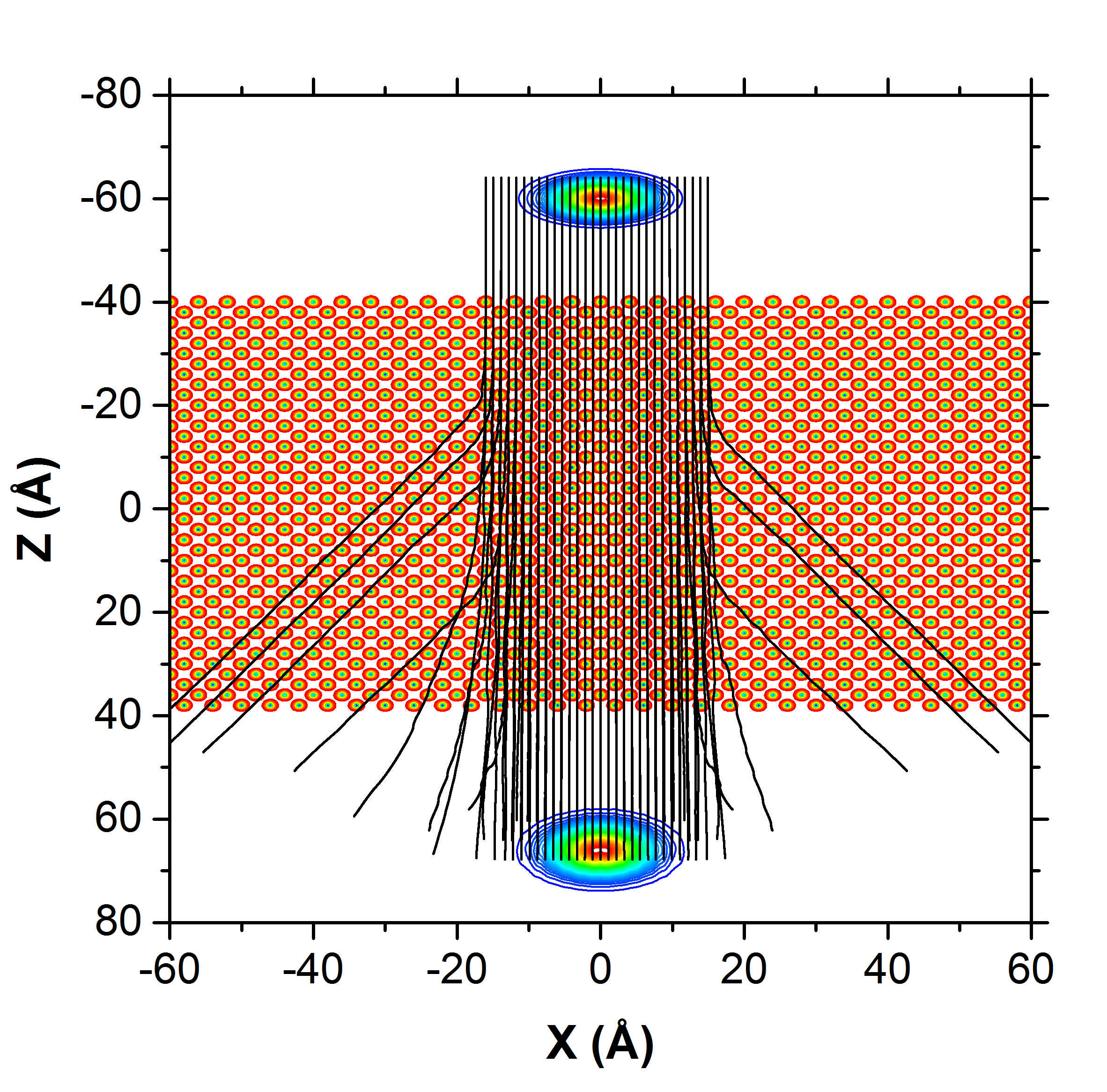
Figure 1: Swarm of Bohmian trajectories simulating the passage of an electron beam through an Al[100] crystal with an incidence energy $E=1$ keV and an angle equal to the Bragg angle $\theta_{B}=2.773^{\circ}$. In this simulation, the electron-crystal interaction potential model consists of 40 atomic layers along the $z$ direction (an average over the $y$ direction, perpendicular to this page, has been considered in passing from the three to the two dimensional model). As a reference, the initial and final probability densities are also represented in terms of contour-plots.

The center of the initial wave function is at $x_{0}=0$ Å and $z_{0}=-60$ Å on the grid and it is propagated vertically with positive momentum in $z$. After passing through the thin Al crystal, a final probability density is retained and plotted. The trajectories begin at the initial positions shown in Fig. 2(a) and their final positions are as in Fig. 2(b) once the simulation is terminated. Each spot indicates the initial or final coordinates of a single trajectory in configuration space. Because of the laminarity displayed by the trajectories (the so-called non-crossing property or rule of Bohmian mechanics Holland (1993); Sanz and Miret-Artés (2012), although it is actually a property of quantum mechanics itself Sanz and Miret-Artés (2008)), there is a direct correlation between the portion of the initial wave packet covered by the Bohmian initial conditions and the final region reached by the corresponding trajectories Sanz and Miret-Artés (2008, 2011), even if we would know nothing about the actual paths. This can be seen by inspecting the initial and final probability densities, which have also been represented in Fig. 2 as contour-plots, and provide a reference on the regions where trajectories start and finalize. Notice that the final positions of the trajectories contribute to the different intensities that would be registered by a detector in a real experiment, since the time-evolution of the swarm of trajectories is in compliance with an exact quantum motion (this does not necessarily mean that real electrons move along these paths, but only their overall or averaged flow), unlike what happens with classical-based methodologies. These peaks represent diffraction spots, which are typically depicted in reciprocal or momentum space. Figures 3(a) and (b) show the probability densities in momentum space at the start and end of the simulation.

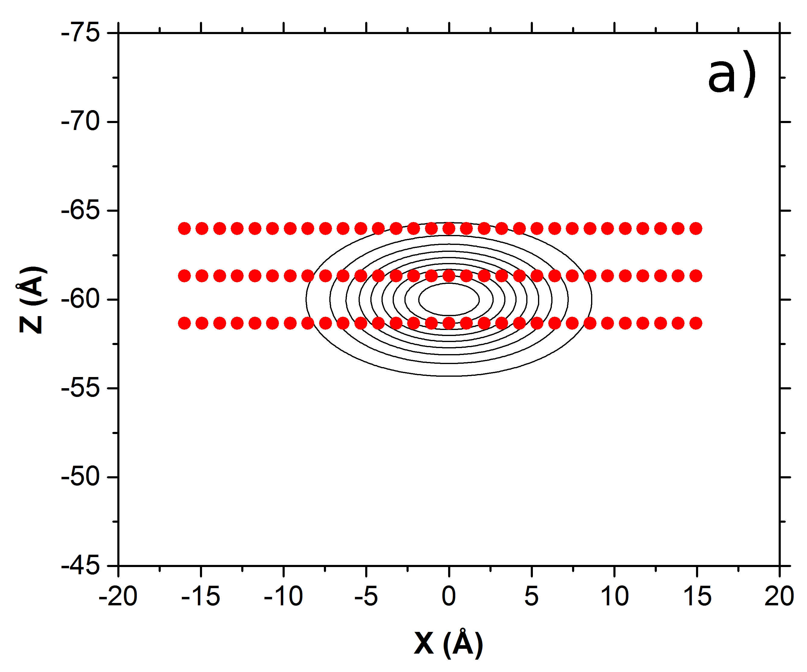
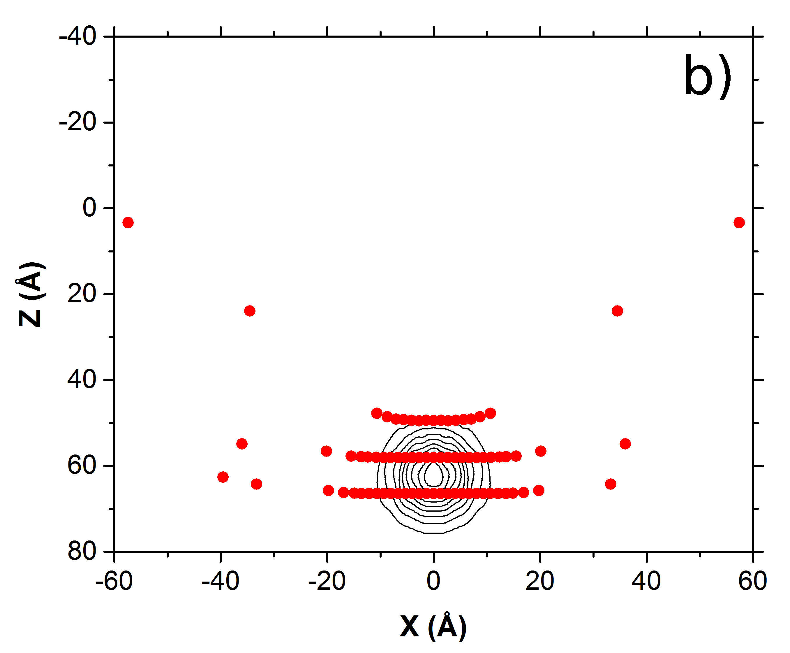
Figure 2: (a) Initial positions for a swarm of Bohmian trajectories sampling the extension covered by the initial probability density (contour-plot). (b) Final positions reached by the trajectories started at the positions displayed in panel (a); the contour-plot of the final probability density is also displayed for the sake of comparison.

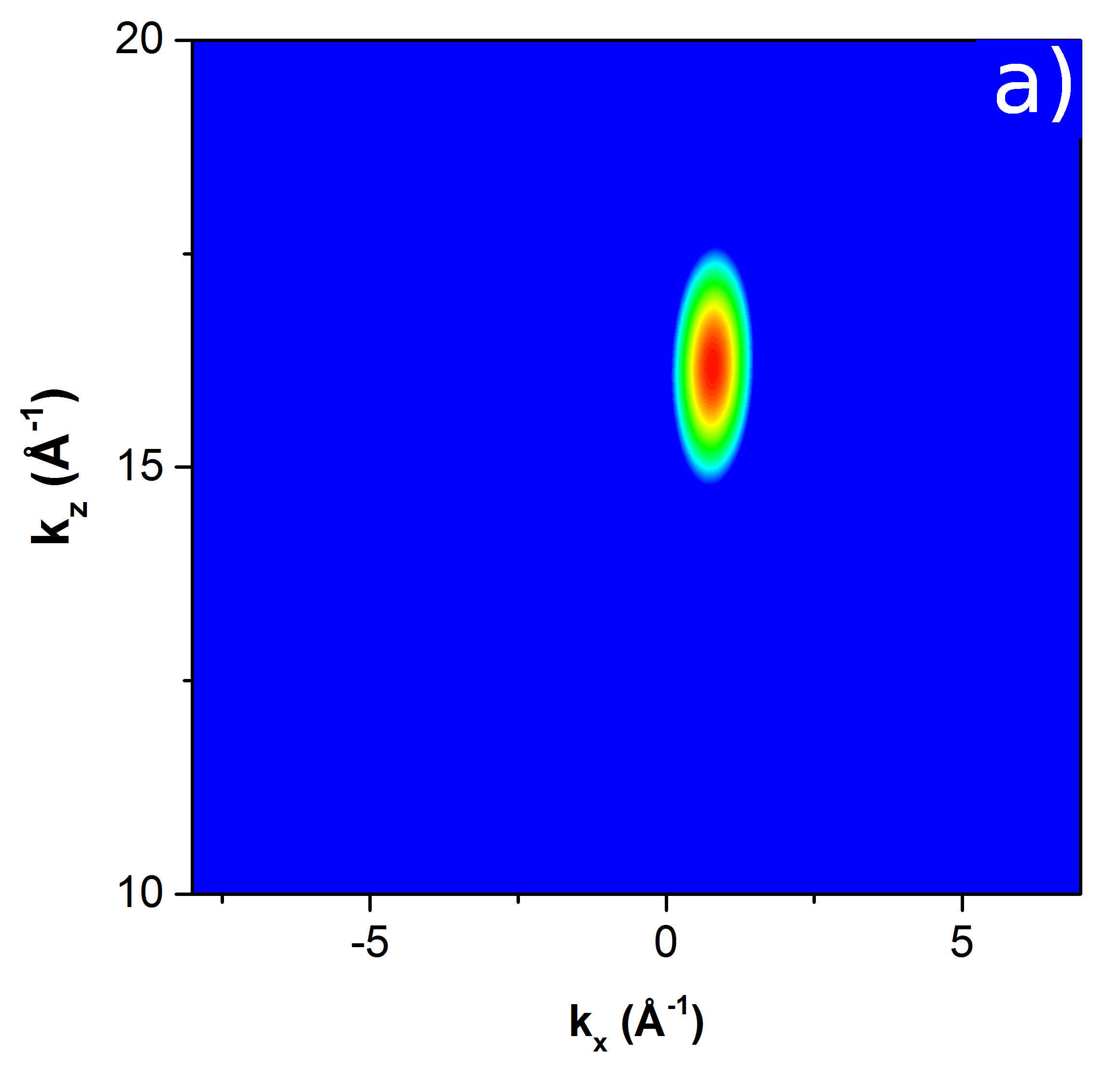
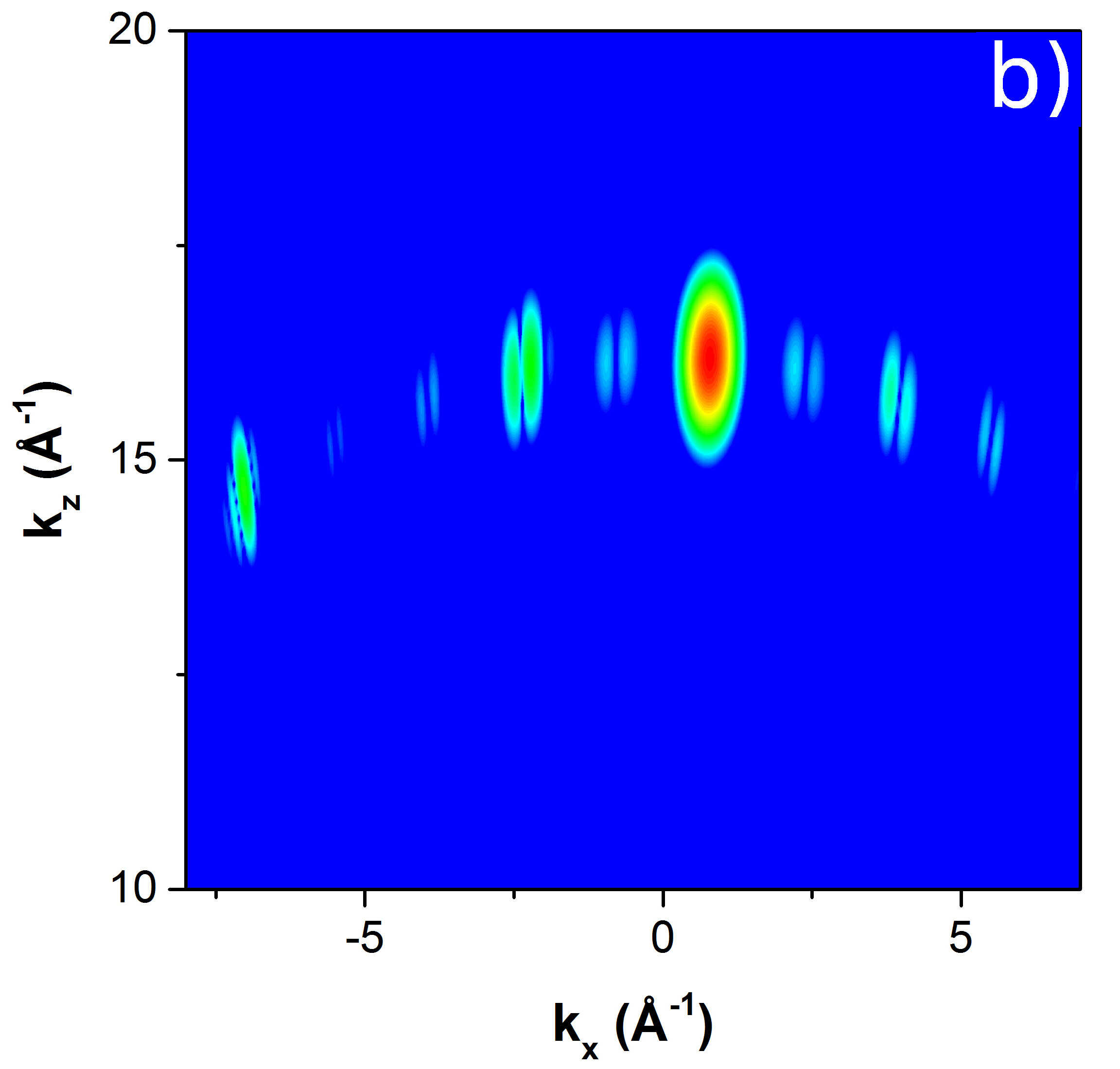
Figure 3: Initial (a) and final (b) probability densities in momentum space for an incidence at the Bragg angle $\theta_{B}\approx-2.773^{\circ}$ with an energy of 1 keV.

Since the initial wave function is a localized wave packet, there is only a primary beam in momentum space. After propagation through the Al single crystal, the beam is diffracted and spots can already be seen in its momentum representation even though the wave function is still in the Fresnel regime. The two adjacent peaks within a single diffraction spot are near-field effects which show that Fresnel diffraction is still apparent. In Fig. 3, the wave packet was tilted to the Bragg condition in order to obtain diffraction spots unique to the crystal. The difference in intensity between certain diffraction spots is a consequence of the atomic configuration of the projected FCC lattice. The alternating sequence of atoms from one layer to another acts as two adjacent gratings where the slits of the second grating are shifted by half a lattice spacing compared to the first. The channels of the second layer cause destructive interference of certain frequencies resulting in less prominent diffraction intensities. However, the only information that can be retained from this data is the intensity distribution of the outgoing wave packet. The trajectories themselves show which portions of the wave function are responsible for these peaks and what occurs inside the material prior to acquisition of this information. The following subsections evaluate the evolution of quantum trajectories for each series of varying initial conditions.

III.1 Probe size

Spot size is highly responsible for resolution in EM. A smaller spot size increases resolution but, as a result, beam broadening can become an issue Cliff and Lorimer (1981). The trajectories at various spot sizes demonstrate what portion of the wave function is responsible for such broadening and how this affects interactions between the electrons and the material, again something arising from the quantum non-crossing mentioned above. Figure 4 shows the propagation of quantum trajectories for two given probe sizes, $\sigma_{x}=0.5a$ and $\sigma_{x}=a$.

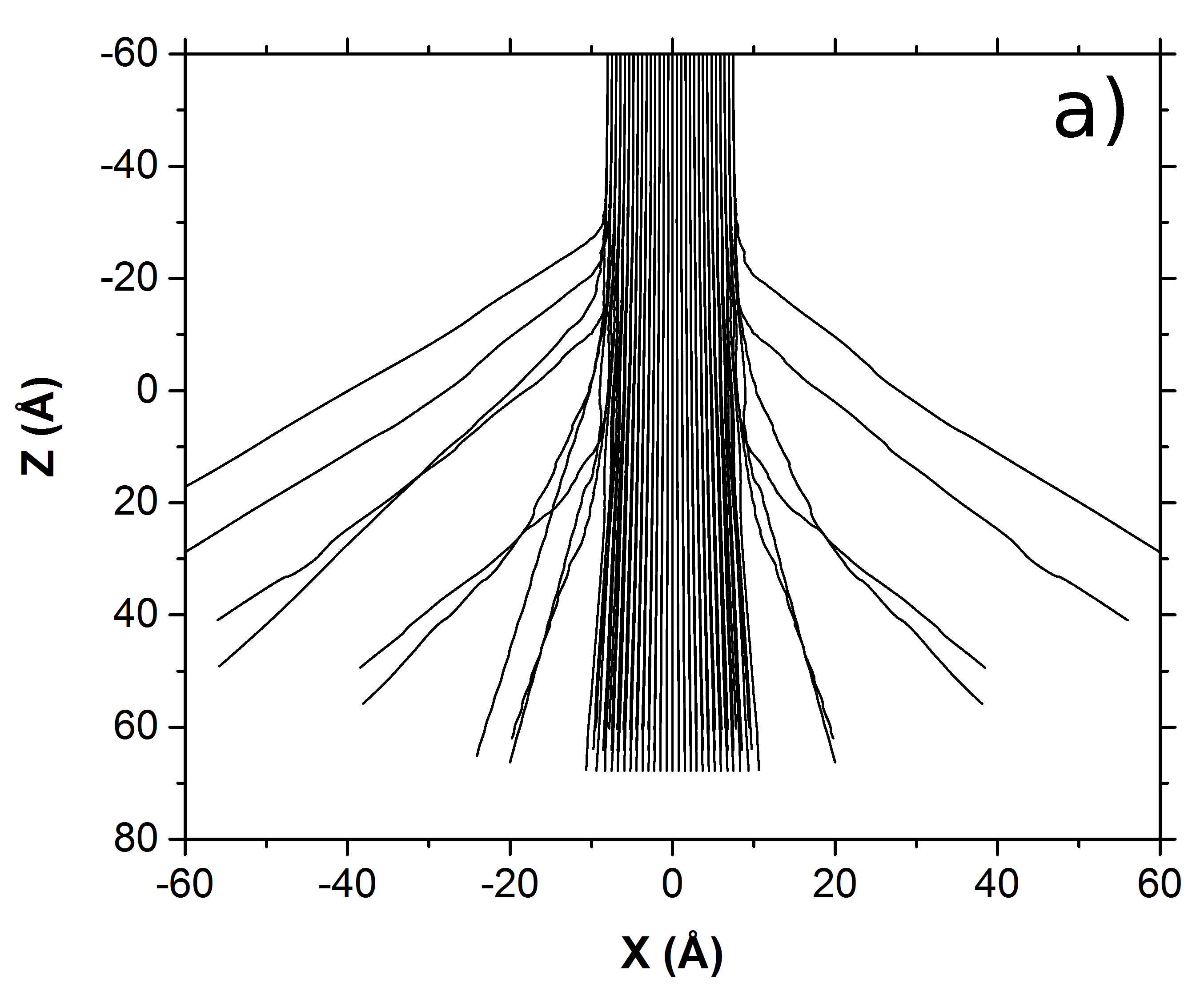
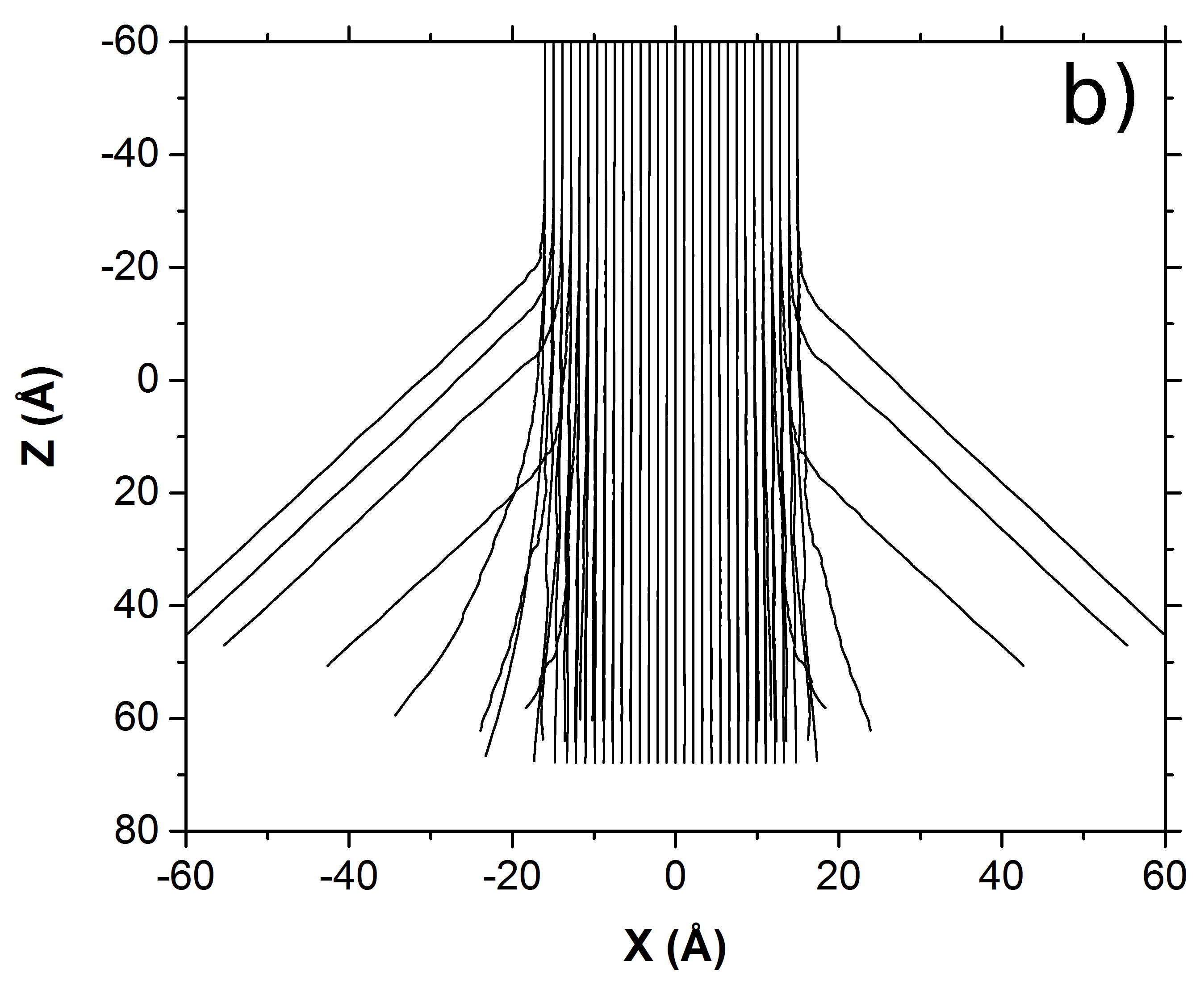
Figure 4: Bohmian trajectories for perpendicular incidence ($\theta_{i}=0^{\circ}$) with 1 keV and two different sizes of the probe: (a) $\sigma_{x}=0.5a$ and (b) $\sigma_{x}=a$.

Given the relatively thin material used with the given voltage of 1 keV, electrons mostly remain in the primary beam upon exit. However, trajectories near $\pm 3\sigma$ and $\pm 4\sigma_{x}$ show the portions of the wave function that are dispersed and contribute to spreading. Comparing Figs. 4(a) and (b) we find that, as is well known from diffraction theory, the broader the incident beam, the lesser the diffraction effects, and vice versa. In terms of trajectories this effect manifests as a larger or smaller amount of trajectories deviating from the incidence direction during the travel through the material, which is followed by a large portion of the incoming swarm of trajectories. Notice that, compared to the multislice technique, it is precisely this deviation which cannot be described, since all trajectories are forced to reach the same slab at the same time due to the reparameterization of the longitudinal coordinate ($z$-direction) in terms of the propagation time. For any Gaussian wave packet, and specifically for an electron beam, the final spread of the wave packet is related to the initial spread by the following,

$$\frac{\sigma}{\sigma_{0}}=\sqrt{1+\frac{\hbar^{2}t^{2}}{4m^{2}\sigma_{0}^{4}}},$$ (10)

with $t$ equal to the time of propagation Bohm (1951). As $\sigma_{0}$ decreases, the ratio of the initial and final spreads increases exponentially until the Fraunhofer region is reached, at which point the relationship becomes linear Sanz and Miret-Artés (2008). This implies that beam broadening of smaller probe sizes is increasingly greater than that of larger probe sizes. The values of $\sigma/\sigma_{0}$ for $\sigma_{0}=0.5a$ and $\sigma_{0}=a$ are 1.46 and 1.02 respectively. Looking at the trajectories, taking the ratio of the average final position in $x$ over the average initial position in $x$ for trajectories that lie within 99% of the Gaussian beam yields 1.42 for $\sigma_{0}=0.5a$ and 1.03 for $\sigma_{0}=a$. This demonstrates that the numerical model is in agreement with analytical theories and the drift of the trajectories is proportional to the wave packet spreading. It is important to note that 99% of the beam broadening is approximately 3$\sigma$ from the mean, indicating that trajectories outside of this range are unlikely to contribute to the broadening. The minimal broadening calculated for the simulation where $\sigma_{0}=a$ can be visualized in Fig. 4(b) where the outlying trajectories do not contribute to the spreading and the trajectories within 99% of beam broadening remain within the same range upon exit. On the other hand, with $\sigma_{0}=0.5a$, the beam spreads by nearly half of the initial probe size regardless of the trajectories outside 99%. In practice, this may cause issues in resolution and data analysis. In all simulations, the initial positions of the trajectories were chosen deterministically whereas the initial wave function has the form of a Gaussian distribution. Therefore, to quantify the average drift of electrons in the beam, a weighted average of the distances between the initial and final positions in $x$ must be used, where the weights are the integral of the initial Gaussian about each starting point. This ensures that the appropriate contributions of each trajectory representative of the wave function are considered. With this, the average drift of trajectories in Fig. 4(b) is 0.0043 Å, while that from Fig. 4(a) is 0.080 Å. A greater drift, and as a result high beam broadening, is still seen at a smaller probe size.

III.2 Tilt angle

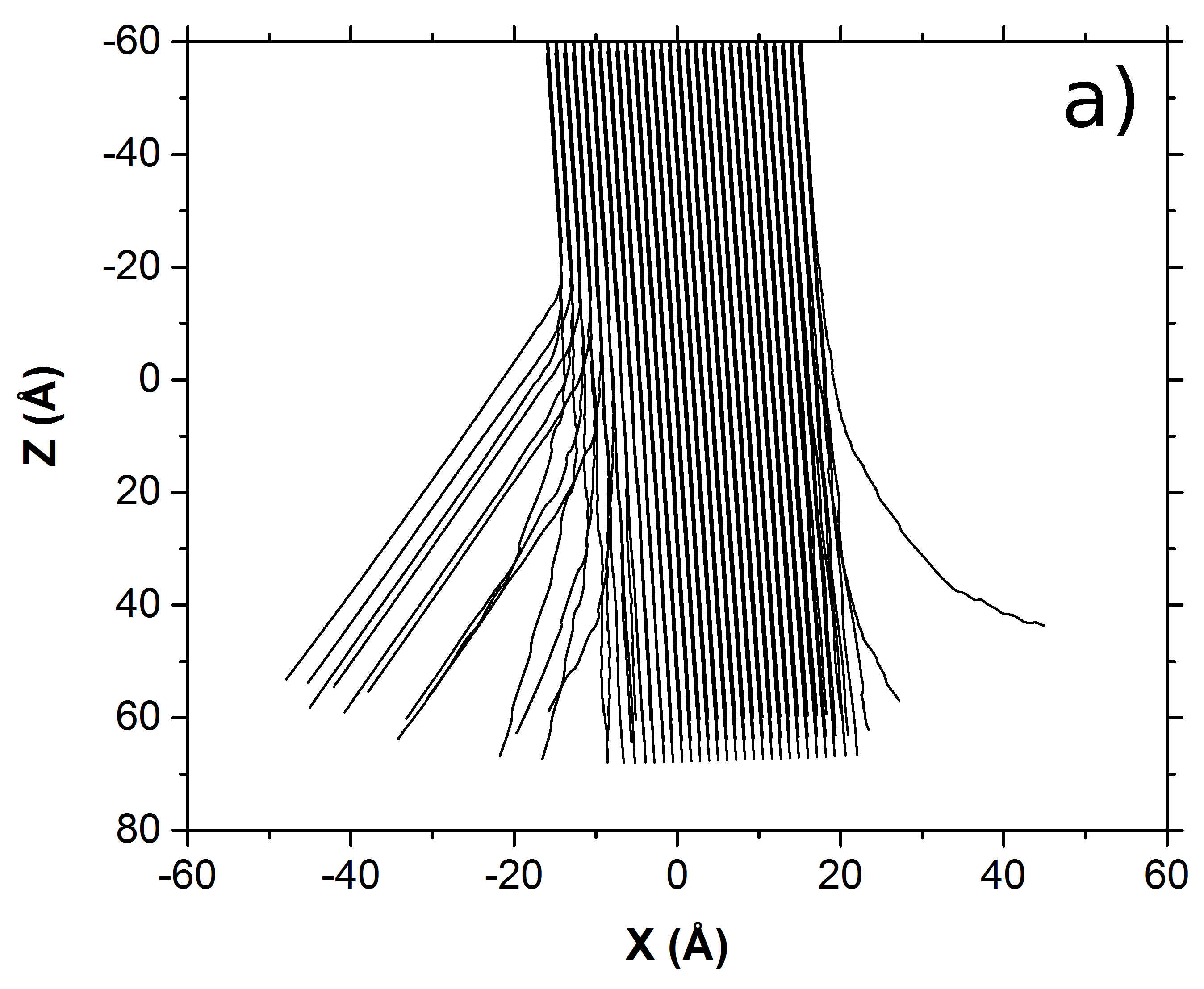
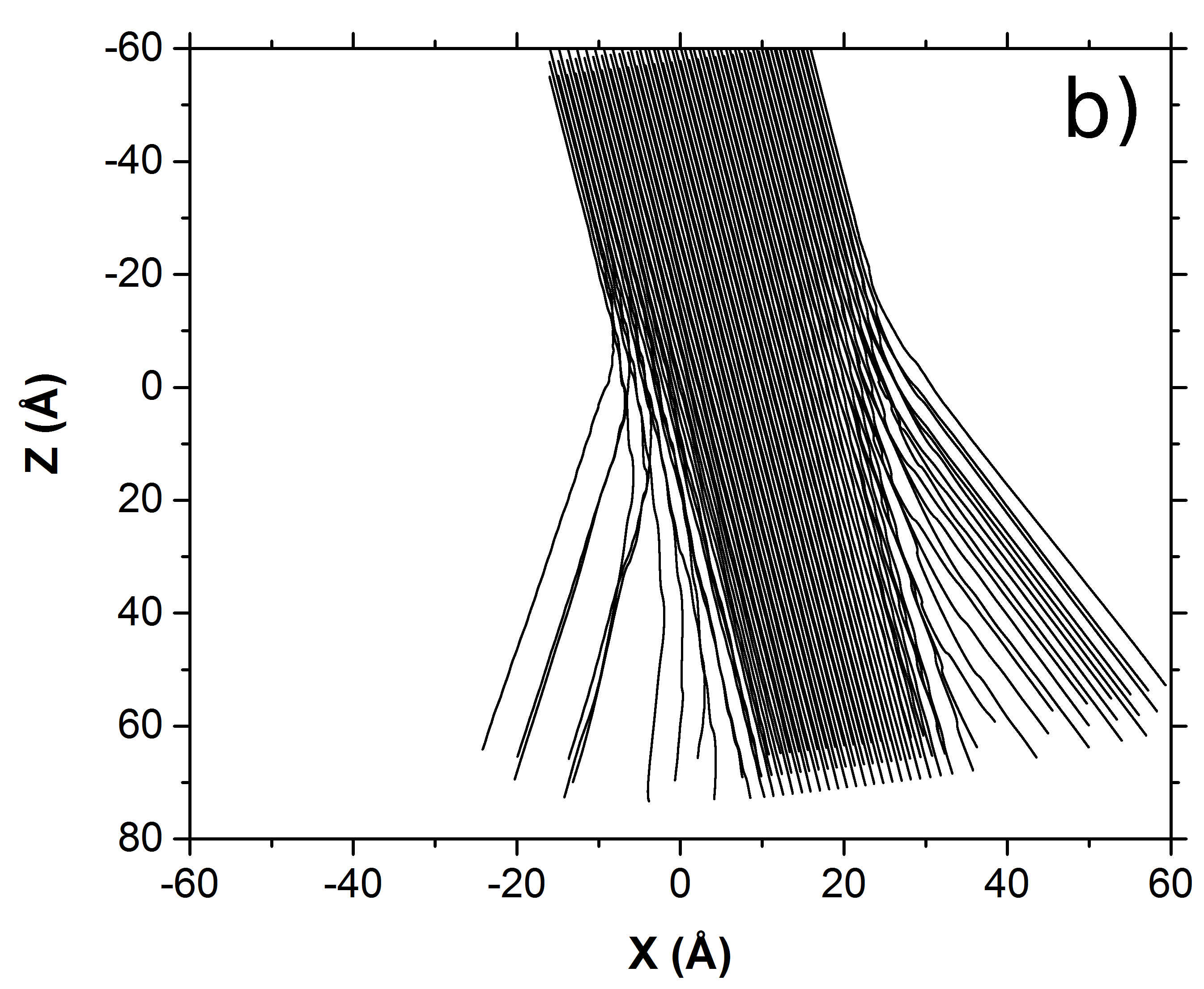
Figure 5: Bohmian trajectories associated with a probe size $\sigma_{x}=a$ for an accelerating voltage of 1 keV and two different incidence angles: (a) a Bragg angle $\theta_{i}=\theta_{B}\approx-2.773^{\circ}$ and (b) $\theta_{i}=-10^{\circ}$.

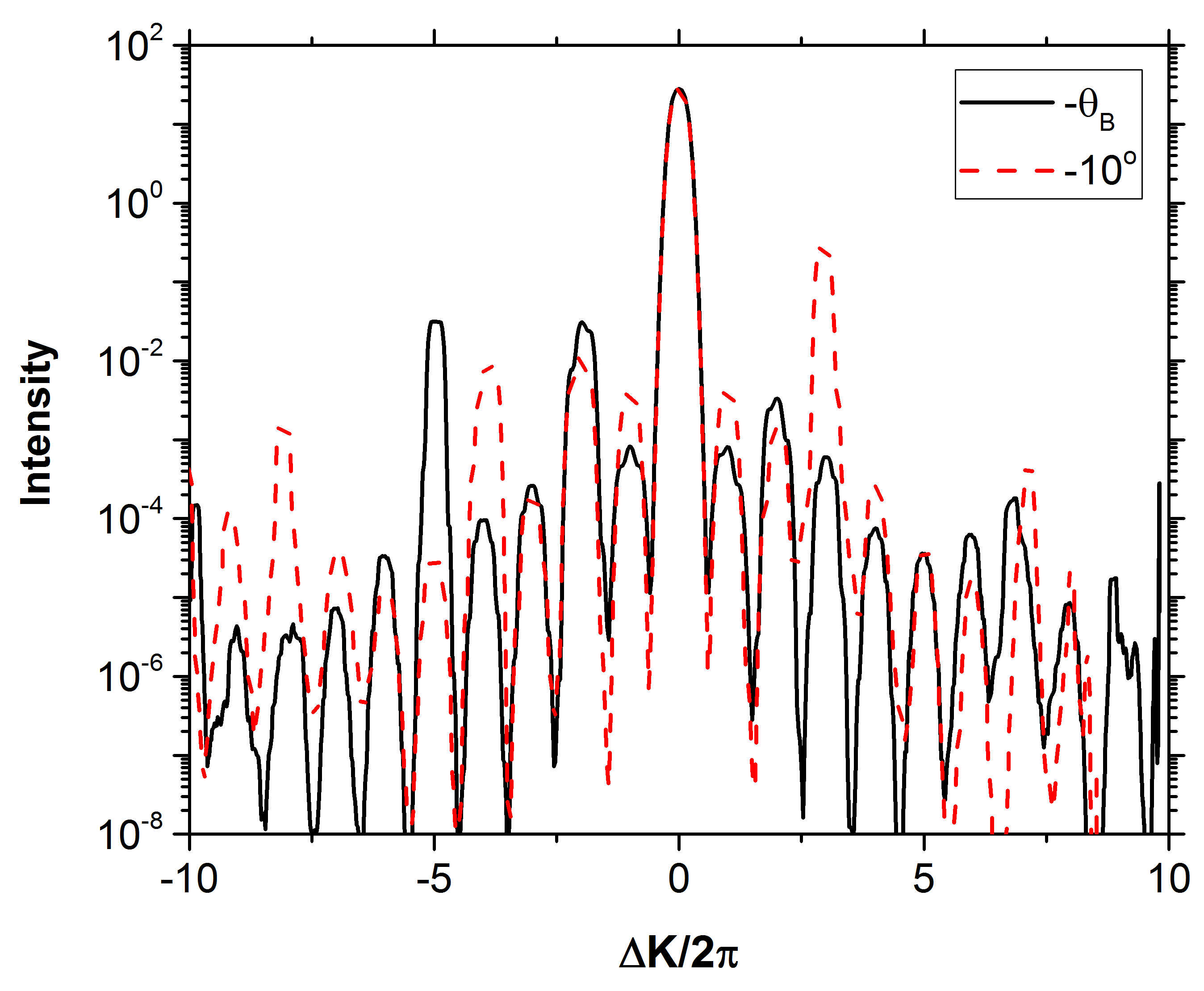
Figure 6: Diffraction intensity distribution as a function of the parallel momentum transferred for two different incidence angles: a Bragg angle $\theta_{i}=\theta_{B}\approx-2.773^{\circ}$ and $\theta_{i}=-10^{\circ}$.

An important advantage of using this method for simulating an electron beam through a thin film is the possibility of reproducing various tilt angles, as shown in Figs. 5(a) and (b). At 1 keV, the Bragg angle is $\theta_{B}\approx-2.773^{\circ}$. This is the condition at which diffraction spots unique to the crystal orientation will appear in the Fraunhofer regime. However, they are still present in Fresnel diffraction and can provide information about the material. Higher tilt angles may be used in experiments such as transmission electron forward scattering diffraction (t-EFSD) where Kikuchi patterns can be imaged Brodusch et al. (2013). Here, any tilt angle can be simulated by rotating the initial wave packet and attributing the appropriate momenta to both spatial components. Then, the portions of the wave function that are either deviated, diffracted or even backscattered by the Al crystal can be distinguished through the trajectories. At a $-10^{\circ}$ tilt, although the Bragg condition is not satisfied, the tail ends of the wave function are still highly deviated. This could be due to dispersion of the wave function as a result of the high incidence angle. As mentioned previously, the thin specimen acts as a grating. The dispersion, $D$, of a grating is calculated by the following.

$$D=\frac{|m|}{b\cos\theta_{0}},$$ (11)

where $b$ is the spacing of the grating, $m$ is the spectral order, and $\theta_{0}$ is the incidence angle Elmore and Heald (1969). As $\theta_{0}$ increases, approaching $\pi/2$, the denominator of Eq. 11 tends to zero and the dispersion increases. This can be observed in Fig. 5(b) by the low densities of coupled trajectories. At the Bragg condition, the portions of the wave function which contribute to the first and second diffraction beams can be discerned by high densities of the coupled portion of trajectories diffracted away from the primary beam. Given the crystal structure, contributions to the second diffraction peak away from the primary beam are greater than those to the first. This is evident by the momentum representation of the wave function in Fig. 3(b) and is further verified by calculation of the diffraction intensity distribution of the final wave function computed through the S-matrix, Fig. 6.

While the primary beam has the highest intensity, the intensity of the second peak is also considerably high. Again, the forbidden reflection of the first diffraction spot is due to the alternating sequence of atomic rows in the crystal. The peak at $\Delta K/2\pi=-2$ is more intense then that at $\Delta K/2\pi=+2$ because of the negative tilt to the Bragg angle. Compared to the intensity distribution of the tilt to $-10^{\circ}$, whose peaks are convoluted indicating incoherent scattering and high dispersion of the beam. The trajectories themselves demonstrate precisely which portion of the wave function contributes to each intensity.

III.3 Accelerating voltage

A beam of electrons interacts very differently with a material depending on the accelerating voltage. While little to no interactions may be seen through thin films at high energies, effects such as backscattering and high angle collisions may be observed at low energies. In EM, the choice of accelerating voltage is highly dependent on the phenomenon being characterized. To reach certain ionization energy levels, accelerating voltages near 20-30 keV are often used for SEM of bulk specimens. On the other hand, these energies are still considerably lower than those used in a TEM. Lower energies may be used for high resolution imaging of small structures such as grains within Al-Li alloys Brodusch et al. (2012). Although these studies are done on bulk materials, it is interesting to investigate the effects of low energies on thin films to make parallels between the two sample types. Therefore, trajectories computed for different accelerating voltages can show at which point the time-dependence of the wave function may or may not be a factor.

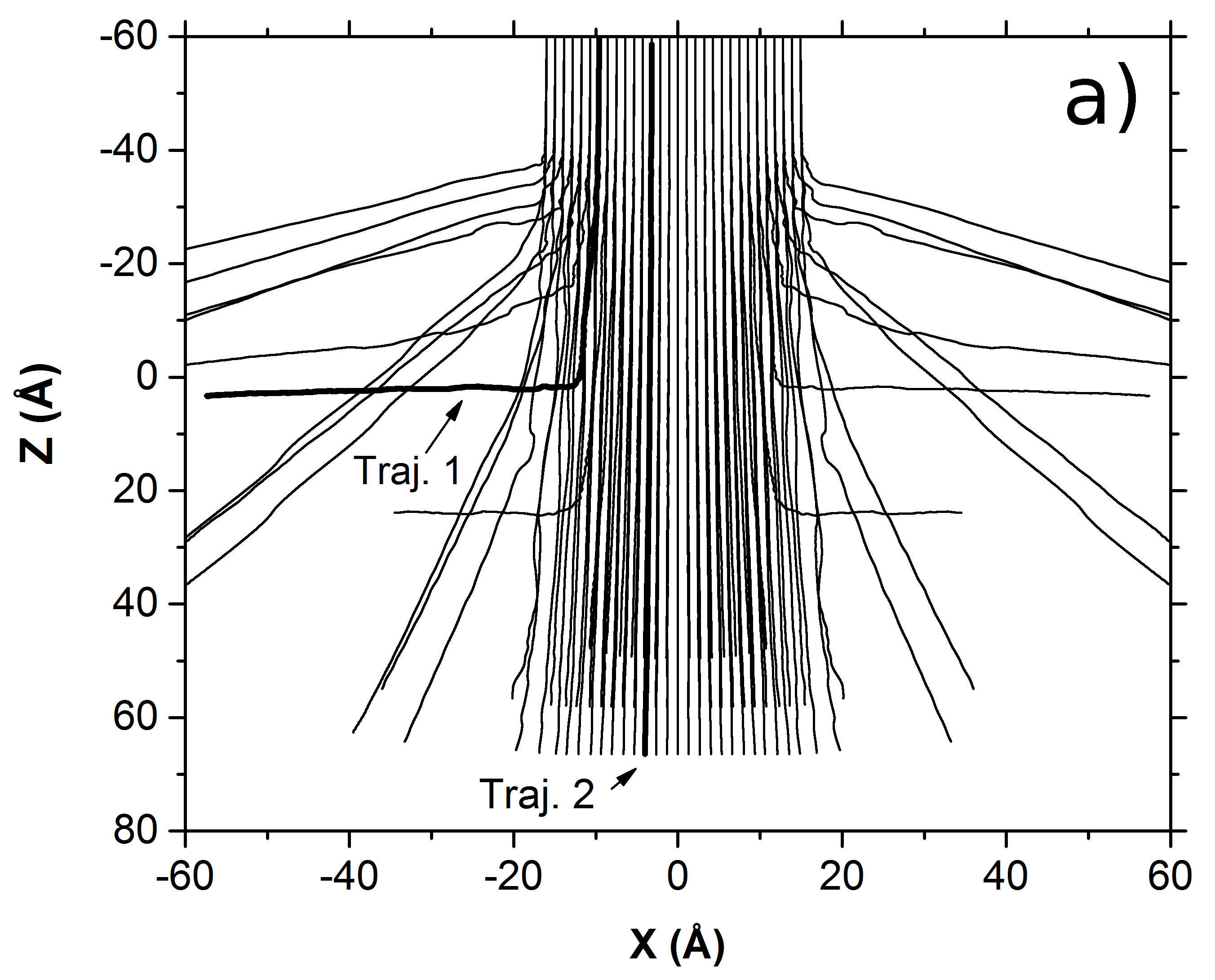
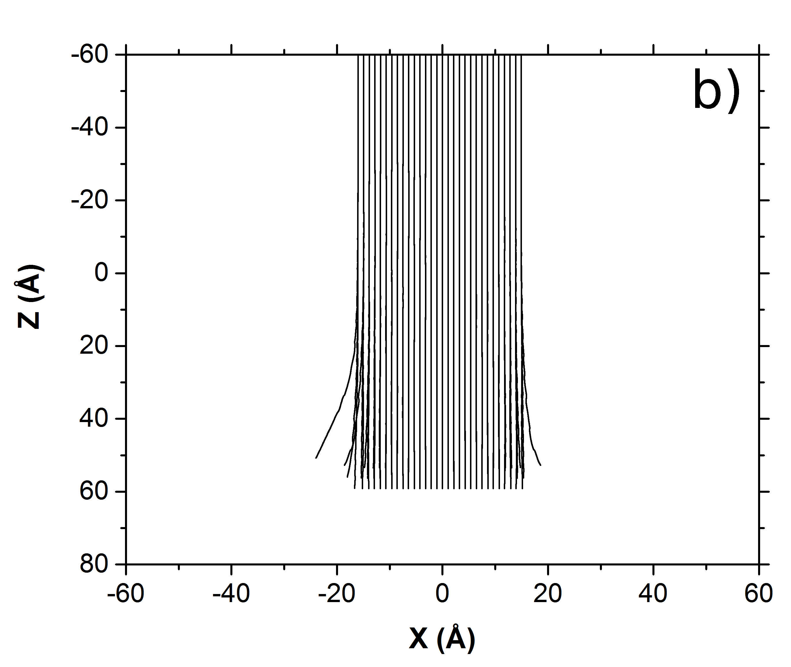
Figure 7: Bohmian trajectories associated with a probe size $\sigma_{x}=a$ for perpendicular incidence ($\theta_{i}=0^{\circ}$) and two different values of the accelerating voltage: (a) 0.1 keV and (b) 6 keV.

Figure 7(b) shows trajectories computed for a wave packet at an energy of 6 keV. It can be seen that there is very little change in the trajectory paths with a few single paths that could be deviated in the far-field. In such a case, the result resembles the trajectories obtained by Zhang et al., where it is assumed that the guiding equations are independent of time and only a constant flow is calculated Zhang et al. (2015). An accelerating voltage of 6 keV is sufficient to show complete transmission of the beam because of the small thickness of the material simulated. There could in fact be scattering at this energy with thicker materials and scattering will always be present in bulk materials. Therefore, a time-independent approach cannot be used if the desire is to investigate various energies or sample thicknesses. In a 20 atom layer sample, 0.1 keV is sufficient to show the presence of backscattering, as in Fig. 7(a), where collisions can cause particles to remain inside the material or even exit the material at the surface of incidence. This is not normally seen in thin materials, however the trajectories at the tail end of the wave function in Fig. 7(a) show a complete transfer of momentum from the $z$-direction to the $x$-direction indicating that in a very small percentage of the incident electrons, some high angle scattering may occur. In this case, the kinetic energy of the trajectories varies considerably compared to trajectories which do not suffer such scattering.

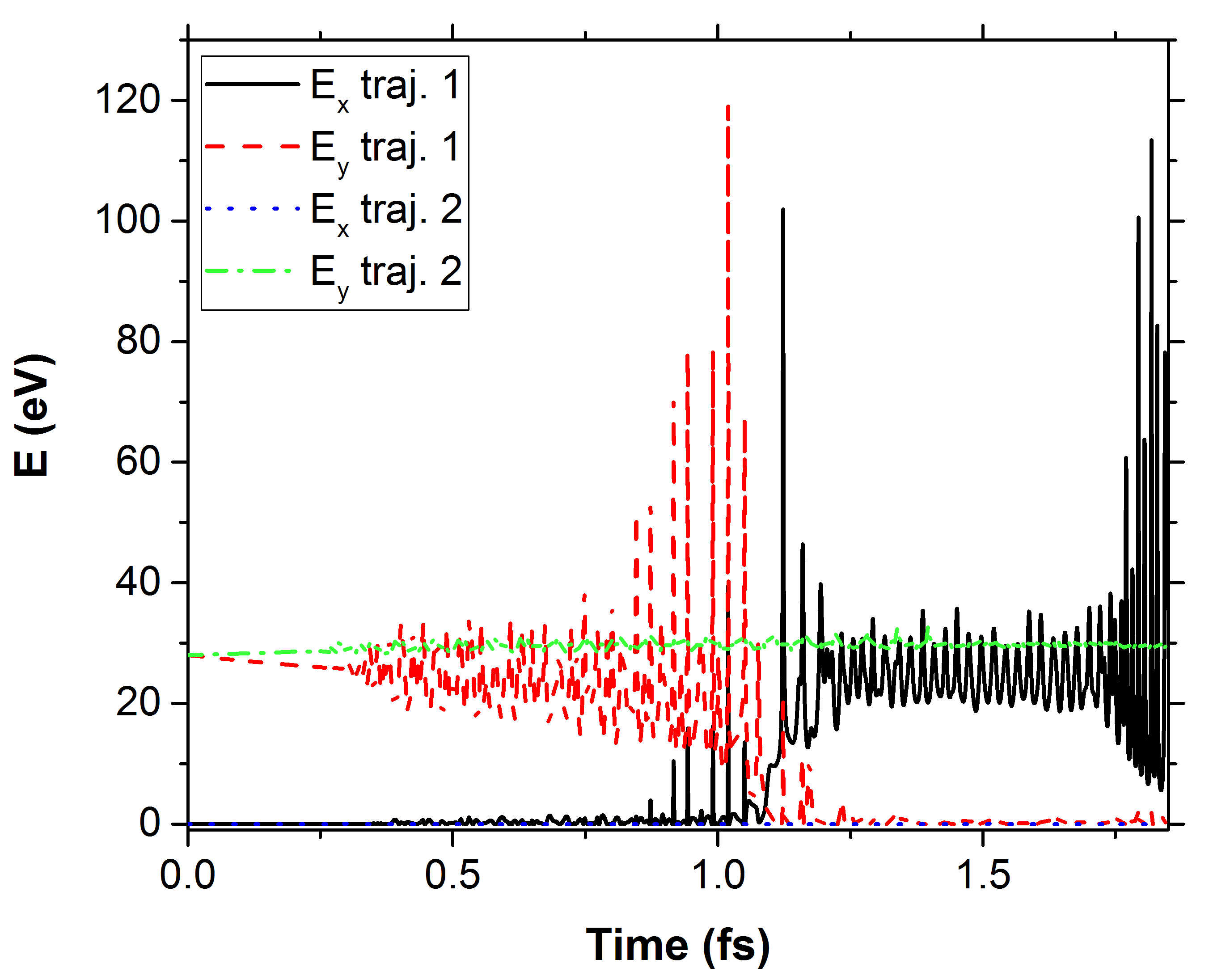
Figure 8: Perpendicular ($z$) and parallel ($x$) components of the kinetic energy for a Bohmian trajectory undergoing a high angle deviation (traj. 1) and another remaining in the primary beam (traj. 2), accelerated by a voltage of 0.1 keV.

This is shown in Fig. 8, where the $x$ and $z$ components of the kinetic energy of a trajectory that is highly deviated are compared to those of one that remains in the primary beam. Trajectories 1 and 2 are indicated in Fig. 7(a). The values are calculated using the momentum, $p$, of the trajectories as $E_{K}=p^{2}/2m$. While both components of trajectory 2 remain relatively constant, with negligible kinetic energy in the $x$-direction, there are high fluctuations in the energy components of trajectory 1. Near 1 fs, there is a transfer of energy between the $z$ and $x$ components. This would indicate the point at which the trajectory’s path deviates towards the $x$-direction. The high fluctuations throughout time in the kinetic energy of trajectory 1 can be attributed to the effects of the crystal potential on this part of the wave function. These backscattering effects could not be reproduced with reduced trajectories which use the multislice algorithm to obtain the corresponding wave function. Conversely, a full physical picture of the electron beam interaction with the material is easily observed through this quantum trajectory method. The difference in propagation between the two accelerating voltages can also be shown by comparing the restricted probabilities Sanz and Miret-Artés (2011), i.e., the space integral of the probability density within a given space region, as given by Eq. (6). Thus, in our case, as mentioned in Sec. II, the regions of interest are delimited by the material slab: before the material (I), inside the material (II), and after the material (III), for both energies as shown in Fig. 9.

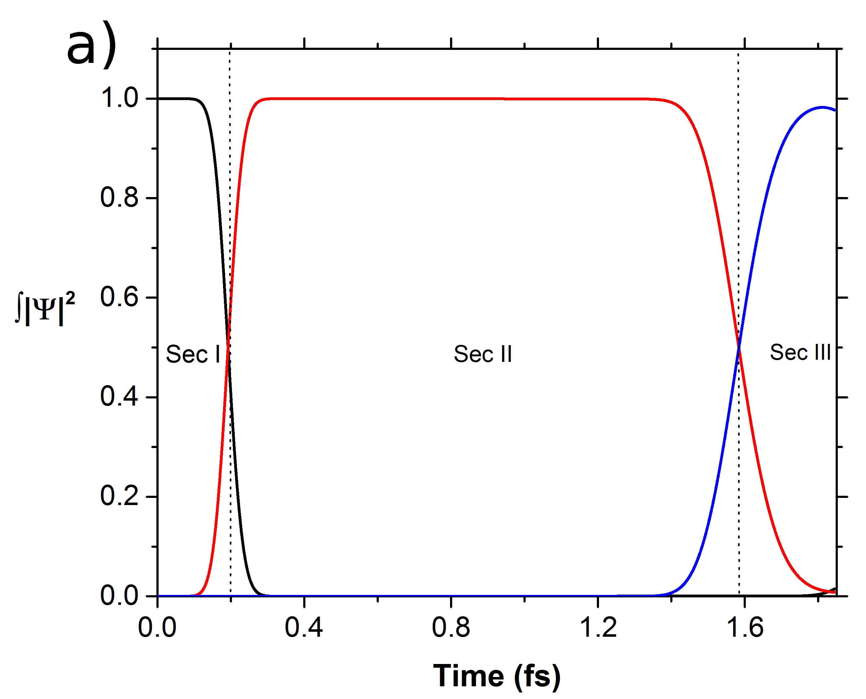
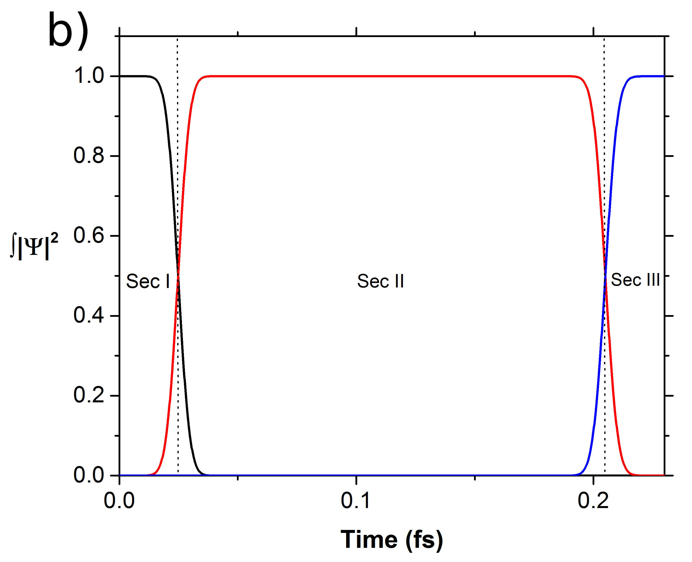
Figure 9: Evolution of the restricted probabilities, as given by Eq. (6), before (I), inside (II) and after (III) the material for two different accelerating voltages: (a) 0.100 keV and (b) 6 keV.

At 6 keV, the probability density is completely transferred to region II after a certain period of time and subsequently transferred to region III at a later time, where these transitions occur very rapidly. However, at 0.1 keV, even though most of the probability density is transferred from region II to region III, this transition is much slower indicating a longer residence time inside the material. With a thicker sample material, this transition may become even slower and the curve associated with region II may not ever reach zero.

IV Conclusions

Simulations of an electron beam through a thin Al single crystal were performed using the theory of Bohmian mechanics. The wave function of a 2D electron beam passing through the material was simulated and quantum trajectories were computed to quantitatively describe the propagation of the wave function. Specifically, this work performs 2D simulations in order to provide preliminary demonstrations of the advantages of this time-dependent method of computing quantum trajectories while retaining some computational efficiency. Extensions into a 3D time-dependent situation or slicing approach are also possible and are investigated in work currently under development. Furthermore, if propagation is continued into the far-field, Fraunhofer diffraction is distinguishable in configuration space when computed by a free particle time evolution of the wave function following its transmission through the material.

Thus, it has been shown that phenomena that are not distinguishable or unambiguous by current diffraction simulation techniques, such as backscattering and the possibility of high angle collisions, can easily be observed by the methodology here employed. It has also been shown that initial conditions, such as low accelerating voltages and high tilt angles by rotation of the initial wave function, can be introduced in the numerical simulation of TEM data analysis, while they are out of scope in other currently existing and widely used methods in the literature.