Conditional Mean and Quantile Dependence Testing in High Dimension

Abstract

Motivated by applications in biological science, we propose a novel test to assess the conditional mean dependence of a response variable on a large number of covariates. Our procedure is built on the martingale difference divergence recently proposed in Shao and Zhang (2014), and it is able to detect certain type of departure from the null hypothesis of conditional mean independence without making any specific model assumptions. Theoretically, we establish the asymptotic normality of the proposed test statistic under suitable assumption on the eigenvalues of a Hermitian operator, which is constructed based on the characteristic function of the covariates. These conditions can be simplified under banded dependence structure on the covariates or Gaussian design. To account for heterogeneity within the data, we further develop a testing procedure for conditional quantile independence at a given quantile level and provide an asymptotic justification. Empirically, our test of conditional mean independence delivers comparable results to the competitor, which was constructed under the linear model framework, when the underlying model is linear. It significantly outperforms the competitor when the conditional mean admits a nonlinear form.

, , and

1 Introduction

Estimation and inference for regression models is of central importance in statistics. For a response variable $Y\in\mathbb{R}$ and a set of covariates $X\in\mathbb{R}^{p}$, it would be desirable to determine whether $X$ is useful in modeling certain aspect of the response, such as the mean or quantiles of $Y$, even before constructing a parametric/nonparametric model. The main thrust of this article is to introduce new tests for conditional mean and quantile dependence in high dimension, which allow the dimension $p$ to be much larger than sample size $n$. Our dependence testing problem in the high dimensional setting is well motivated by an important problem in biological science, which is to test for the significance of a gene set and identify significant sets of genes that are associated with certain clinical outcomes; see Subramanian et al. (2005), Efron and Tibshirani (2007) and Newton et al. (2007), among others. Since the size of a gene set can range from a few to thousands, this calls for a simultaneous test that can accommodate high dimensional covariates and possible dependence within the covariates.

Recently, Zhong and Chen (2011) proposed a simultaneous test for coefficient in high dimensional linear regression. Specifically, for a univariate response $Y$ and high dimensional covariates $X\in\mathbb{R}^{p}$, they assume $\mathbb{E}(Y|X)=\alpha+X^{T}\beta$ and ${\mbox{var}}(Y|X)=\sigma^{2}$, and test $H_{0}:\beta=\beta_{0}$ versus $H_{a}:\beta\not=\beta_{0}$ for a specific $\beta_{0}\in\mathbb{R}^{p}$ based on a random sample from the joint distribution of $(X,Y)$. A special case of primary interest is when $\beta_{0}=0$, which indicates insignificance of all covariates. However, the assumption of a high dimensional linear model seems quite strong and we are not aware of any procedure to validate this linear model assumption in the high dimensional setting. To assess the usefulness of the covariates $X$ in modeling the mean of $Y$, we effectively want to test

$$H_{0}:\mathbb{E}(Y|X)=\mathbb{E}(Y)~{}\mbox{almost surely},~{}\mbox{versus}~{}H_{a}:P(\mathbb{E}(Y|X)=\mathbb{E}(Y))<1,$$

in other words, the conditional mean independence of $Y$ on $X$. Thus it seems desirable to develop a test that can accommodate the high dimensionality and dependence in the covariates without assuming a linear (or parametric) model. It turns out that the above testing problem in a model-free setting is very challenging since the class of alternative we target is huge owing to the growing dimension and nonlinear dependence.

To circumvent the difficulty, we focus on testing the weak null hypothesis:

$$H_{0}^{\prime}:\mathbb{E}[Y|x_{j}]=\mathbb{E}[Y]\quad\text{almost surely},~{}\text{for all}~{}1\leq j\leq p,$$

where $X=(x_{1},\cdots,x_{p})^{T}$, which is itself an interesting and meaningful testing problem; see Section 2 for more discussions. Since $H_{0}$ implies $H_{0}^{\prime}$, a rejection of $H_{0}^{\prime}$ automatically rejects $H_{0}$. Furthermore, $H_{0}$ and $H_{0}^{\prime}$ are equivalent in the framework of high dimensional linear models under some mild assumptions; see Example 2.1. In this paper, we propose a new test for $H_{0}^{\prime}$, i.e., the conditional mean independence for each $x_{j}$, that can allow high dimensionality and dependence in $X$ without any parametric or homoscedastic model assumption. Our test statistic is built on the so-called martingale difference divergence (MDD, hereafter) [Shao and Zhang (2014)], which fully characterizes the conditional mean independence of a univariate response on the covariates of arbitrary dimension. For any random variable ${\mathcal{Y}}$ and random vector ${\mathcal{X}}$, the MDD is defined as the weighted $L_{2}$ norm of ${\mbox{cov}}({\mathcal{Y}},e^{\imath<s,{\mathcal{X}}>})$ with $\imath=\sqrt{-1}$ and the weighting function similar to the one used in distance covariance [Székely, Rizzo and Bakirov (2007)], and thus inherits many desirable properties of distance covariance; see Shao and Zhang (2014) and Park et al. (2015) for more details. Theoretically, we establish the asymptotic normality of our MDD-based test statistic under suitable assumption on the eigenvalues of a Hermitian operator constructed based on the characteristic functions of the covariates. These conditions can be further simplified under banded dependence structure on the covariates or Gaussian design. The theoretical results are of independent interest since they provide some insights on the asymptotic behavior of $U$-statistic in high dimension. From a practical viewpoint, our test does not involve any tuning parameter and uses standard $z$ critical value, so it can be conveniently implemented. To reduce the finite sample size distortion, we further propose a studentized wild bootstrap approach and justify its consistency. Simulation results show that the wild bootstrap leads to more accurate size for most cases, at the expense of additional computation.

For heterogeneous data where ${\mbox{var}}(Y|X)$ is not a constant, conditional quantiles of $Y$ given $X$ can provide additional information not captured by conditional mean in describing the relationship between $Y$ and $X$. Quantile regression [Koenker and Bassett (1978)] has evolved into a quite mature area of research over the past several decades. For high dimensional heterogeneous data, quantile regression models continue to be useful; see Wang, Wu and Li (2012) and He, Wang and Hong (2013) for recent contributions. For the use of quantile based models and methods in genomic data analysis, see Wang and He (2007, 2008), among others. Motivated by the usefulness of conditional quantile modeling, we propose to extend the test for conditional mean independence $H_{0}^{\prime}$ and introduce a test for conditional quantile independence at a particular quantile level $\tau\in(0,1)$. It is worth mentioning that we are not aware of any tests in the literature developed for conditional quantile independence in the high dimensional setting.

There is a recent surge of interest in inference for regression coefficients in high dimensional setting, as motivated by the emergence of high-dimensional data in various scientific areas such as medical imaging, atmospheric and climate sciences, and biological science. The analysis of high-dimensional data in the regression framework is challenging due to the high dimensionality of covariates, which can greatly exceed the sample size, and traditional statistical methods developed for low and fixed-dimensional covariates may not be applicable to modern large data sets. Here we briefly mention some related work on testing for dependence or the significance of regression coefficients in high dimensional regression setting. Yata and Aoshima (2013) proposed a simultaneous test for zero correlation between $Y$ and each component of $X$ in a nonparametric setting; Feng, Zou and Wang (2013) proposed a rank-based test building on the one in Zhong and Chen (2011) under the linear model assumption; Testing whether a subset of $X$ is significant or not after controlling for the effect of the remaining covariates is addressed in Wang and Cui (2013) and Lan, Wang and Tsai (2014); Székely and Rizzo (2013) studied the limiting behavior of distance correlation [Székely, Rizzo and Bakirov (2007)] based test statistic for independence test when the dimensions of $Y$ and $X$ both go to infinity while holding sample size fixed; Goeman et al. (2006) introduced a score test against a high dimensional alternative in an empirical Bayesian model.

It should be noted that our testing problem is intrinsically different from the marginal feature screening problem in terms of the formulation, goal and methodology. The marginal screening has been extensively studied in the literature since Fan and Lv’s (2008) seminal work; see Liu, Zhong and Li (2015) for an excellent recent review. Generally speaking, marginal screening aims to rank the covariates using sample marginal utility (e.g., sample MDD), and reduce the dimension of covariates to a moderate scale, and then perform variable selection using LASSO etc. For example, if we use MDD as the marginal utility, as done in Shao and Zhang (2014), we then screen out the variables that do not contribute to the mean of $Y$. The success of the feature screening procedure depends on whether the subset of kept variables is able to contain the set of all the important variables, which is referred as the sure screening consistency in theoretical investigations. For the testing problem we address in this paper, we aim to detect conditional mean dependence of $Y$ on $X$, and the formulation and the output of the inference is very different from that delivered by the marginal screening. In practice, the testing can be conducted prior to model building, which includes marginal screening as an initial step. In particular, if our null hypothesis holds, then there is no need to do marginal screening using MDD, as the mean of the response does not depend on covariates. It is worth noting that our test is closely tied to the adaptive resampling test of McKeague and Qian (2015), who test for the marginal uncorrelatedness of $Y$ with $x_{j}$, for $j=1,\cdots,p$ in a linear regression framework. We shall leave a more detailed discussion of the connection and difference of two papers and numerical comparison to the supplement.

The rest of the paper is organized as follows. We propose the MDD-based conditional mean independence test and study its asymptotic properties in Section 2. We describe a testing procedure for conditional quantile independence in Section 3. Section 4 is devoted to numerical studies. Section 5 concludes. The technical details, extension to factorial designs, additional discussions and numerical results are gathered in the supplementary material.

2 Conditional mean dependence testing

For a scalar response variable $Y$ and a vector predictor $X=(x_{1},\dots,x_{p})^{T}\in\mathbb{R}^{p}$, we are interested in testing the null hypothesis

$$H_{0}:\mathbb{E}[Y|x_{1},\dots,x_{p}]=\mathbb{E}[Y]\quad\text{almost surely}.$$ (1)

Notice that under $H_{0}$, we have $\mathbb{E}[Y|x_{j}]=\mathbb{E}[Y]$ for all $1\leq j\leq p$. This observation motivates us to consider the following hypothesis

$$H_{0}^{\prime}:\mathbb{E}[Y|x_{j}]=\mathbb{E}[Y]\quad\text{almost surely},$$ (2)

for all $1\leq j\leq p$ versus the alternative that

$$H_{a}^{\prime}:P(\mathbb{E}[Y|x_{j}]\neq\mathbb{E}[Y])>0$$ (3)

for some $1\leq j\leq p.$ We do not work directly on the original hypothesis in (1), because a MDD-based testing procedure targeting for the global null $H_{0}$ generally fails to capture the nonlinear conditional mean dependence when $p$ is large; see Remark 2.2 for more detailed discussions. In addition, if we regard $\mathbb{E}[Y|x_{j}]-\mathbb{E}[Y]$ as the main effect of $x_{j}$ contributing to the mean of $Y$, then it seems reasonable to test for the nullity of main effects first, before proceeding to the higher-order interactions, in a manner reminiscent of “Effect Hierarchy Principle” and “Effect Heredity Principle” in design of experiment [see pages 172-173 of Wu and Hamada (2009)]. Testing $H_{0}^{\prime}$ versus $H_{a}^{\prime}$ is a problem of own interest from the viewpoint of nonparametric regression modeling, where additive and separate effects from each $x_{j}$ usually first enter into the model before adding interaction terms.

In some cases, $\mathbb{E}[Y|x_{j}]=0$ almost surely for $1\leq j\leq p$ implies that $\mathbb{E}[Y|x_{1},\dots,x_{p}]=0$ almost surely.

Example 2.1.

Consider a linear regression model

$$Y=\beta_{1}x_{1}+\beta_{2}x_{2}+\cdots+\beta_{p}x_{p}+\epsilon,$$

where $X=(x_{1},\dots,x_{p})^{T}$ follows the elliptical distribution $EC_{p}(0,\Sigma_{0},\phi_{0})$ with $\phi_{0}$ being the so-called characteristic generator of $X$ and $\Sigma_{0}=(\sigma_{0,ij})^{p}_{i,j=1}$ [see e.g. Fang et al. (1990)], and $\epsilon$ is independent of $X$ with $\mathbb{E}\epsilon=0.$ Under the elliptical distribution assumption, we have

$$\mathbb{E}[Y|x_{j}]=\sum^{p}_{k=1}\beta_{k}\mathbb{E}[x_{k}|x_{j}]=\sum^{p}_{k=1}\beta_{k}\frac{\sigma_{0,jk}}{\sigma_{0,jj}}x_{j}.$$

Thus $\mathbb{E}[Y|x_{j}]=0$ almost surely implies that $\sum^{p}_{k=1}\beta_{k}\sigma_{0,jk}=0$ for all $1\leq j\leq p.$ Writing this in matrix form, we have $\Sigma_{0}\beta=\mathbf{0}_{p\times 1}$ for $\beta=(\beta_{1},\dots,\beta_{p})^{T}$, which suggests that $\beta=\mathbf{0}_{p\times 1}$ provided that $\Sigma_{0}$ is non-singular. In this case, testing $H_{0}$ is equivalent to testing its marginal version $H_{0}^{\prime}$. In particular, the above result holds if $X$ follows a multivariate normal distribution with mean zero and covariance $\Sigma_{0}.$

To characterize the conditional mean (in)dependence, we consider the MDD proposed in Shao and Zhang (2014). Throughout the following discussions, we let ${\mathcal{Y}}$ be a generic univariate random variable and ${\mathcal{X}}$ be a generic $q$-dimensional random vector (e.g. ${\mathcal{X}}=X$ and $q=p$, or ${\mathcal{X}}=x_{j}$ for some $1\leq j\leq p$ and $q=1$). Let $L(y,y^{\prime})=(y-y^{\prime})^{2}/2$ and $K(x,x^{\prime})=|x-x^{\prime}|_{q}$ with $|\cdot|_{q}$ denoting the Euclidean norm of $\mathbb{R}^{q}$. Under finite second moment assumptions on ${\mathcal{Y}}$ and ${\mathcal{X}}$, the MDD which characterizes the conditional mean dependence of ${\mathcal{Y}}$ given ${\mathcal{X}}$ is defined as

$$\begin{split}MDD({\mathcal{Y}}|{\mathcal{X}})^{2}=&\mathbb{E}[K({\mathcal{X}},{\mathcal{X}}^{\prime})L({\mathcal{Y}},{\mathcal{Y}}^{\prime})]+\mathbb{E}[K({\mathcal{X}},{\mathcal{X}}^{\prime})]\mathbb{E}[L({\mathcal{Y}},{\mathcal{Y}}^{\prime})]\\ &-2\mathbb{E}[K({\mathcal{X}},{\mathcal{X}}^{\prime})L({\mathcal{Y}},{\mathcal{Y}}^{\prime\prime})]\\ =&-\mathbb{E}[({\mathcal{Y}}-\mathbb{E}{\mathcal{Y}})({\mathcal{Y}}^{\prime}-\mathbb{E}{\mathcal{Y}}^{\prime})|{\mathcal{X}}-{\mathcal{X}}^{\prime}|_{q}],\end{split}$$ (4)

where $({\mathcal{X}}^{\prime},{\mathcal{Y}}^{\prime})$ and $({\mathcal{X}}^{\prime\prime},{\mathcal{Y}}^{\prime\prime})$ denote independent copies of $({\mathcal{X}},{\mathcal{Y}})$; see Shao and Zhang (2014) and Park et al. (2015). The MDD is an analogue of distance covariance introduced in Székely, Rizzo and Bakirov (2007) in that the same type of weighting function is used in its equivalent characteristic function-based definition and it completely characterizes the conditional mean dependence in the sense that $MDD({\mathcal{Y}}|{\mathcal{X}})=0$ if and only if $E({\mathcal{Y}}|{\mathcal{X}})=E({\mathcal{Y}})$ almost surely; see Section 2 of Shao and Zhang (2014). Note that the distance covariance is used to measure the dependence, whereas MDD is for conditional mean dependence.

In this paper, we introduce a new testing procedure based on an unbiased estimator of $MDD({\mathcal{Y}}|{\mathcal{X}})^{2}$ in the high dimensional regime. Compared to the modified $F$-test proposed in Zhong and Chen (2011), our procedure is model-free and is able to detect nonlinear conditional mean dependence. Moreover, the proposed method is quite useful for detecting “dense” alternatives, i.e., there are a large number of (possibly weak) signals, and it can be easily extended to detect conditional quantile (in)dependence at a given quantile level (see Section 3). It is also worth mentioning that our theoretical argument is in fact applicable to testing procedures based on a broad class of dependence measures including MDD as a special case [see e.g. Székely et al. (2007) and Sejdinovick et al. (2013)].

2.1 Unbiased estimator

Given $n$ independent observations $({\mathcal{X}}_{i},{\mathcal{Y}}_{i})^{n}_{i=1}$ from the joint distribution of $({\mathcal{X}},{\mathcal{Y}})$ with ${\mathcal{X}}_{i}=({\mathcal{X}}_{i1},{\mathcal{X}}_{i2},\dots,{\mathcal{X}}_{iq})^{T}\in\mathbb{R}^{q}$ and ${\mathcal{Y}}_{i}\in\mathbb{R}$, an unbiased estimator for $MDD({\mathcal{Y}}|{\mathcal{X}})^{2}$ can be constructed using the idea of $\mathcal{U}$-centering [Székely and Rizzo (2014); Park et al. (2015)]. Define $A=(A_{ij})^{n}_{i,j=1}$ and $B=(B_{ij})^{n}_{i,j=1}$, where $A_{ij}=|{\mathcal{X}}_{i}-{\mathcal{X}}_{j}|_{q}$ and $B_{ij}=|{\mathcal{Y}}_{i}-{\mathcal{Y}}_{j}|^{2}/2.$ Following Park et al. (2015), we define the $\mathcal{U}$-centered versions of $A_{ij}$ and $B_{ij}$ as

$$\widetilde{A}_{ij}=A_{ij}-\frac{1}{n-2}\sum^{n}_{l=1}A_{il}-\frac{1}{n-2}\sum^{n}_{k=1}A_{kj}+\frac{1}{(n-1)(n-2)}\sum_{k,l=1}^{n}A_{kl},$$

$$\widetilde{B}_{ij}=B_{ij}-\frac{1}{n-2}\sum^{n}_{l=1}B_{il}-\frac{1}{n-2}\sum^{n}_{k=1}B_{kj}+\frac{1}{(n-1)(n-2)}\sum_{k,l=1}^{n}B_{kl}.$$

A suitable estimator for $MDD({\mathcal{Y}}|{\mathcal{X}})^{2}$ is given by

$$MDD_{n}({\mathcal{Y}}|{\mathcal{X}})^{2}=(\widetilde{A}\cdot\widetilde{B}):=\frac{1}{n(n-3)}\sum_{i\neq j}\widetilde{A}_{ij}\widetilde{B}_{ij},$$

where $\widetilde{A}=(\widetilde{A}_{ij})_{i,j=1}^{n}$ and $\widetilde{B}=(\widetilde{B}_{ij})_{i,j=1}^{n}$. In Section 1.1 of the supplement, we show that $MDD_{n}({\mathcal{Y}}|{\mathcal{X}})^{2}$ is indeed an unbiased estimator for $MDD({\mathcal{Y}}|{\mathcal{X}})^{2}$ and it has the expression

$$MDD_{n}({\mathcal{Y}}|{\mathcal{X}})^{2}=\frac{1}{\binom{n}{4}}\sum_{i<j<q<r}h(\mathcal{Z}_{i},\mathcal{Z}_{j},\mathcal{Z}_{q},\mathcal{Z}_{r}),$$

where

$$h(\mathcal{Z}_{i},\mathcal{Z}_{j},\mathcal{Z}_{q},\mathcal{Z}_{r})=\frac{1}{6}\sum_{s<t,u<v}^{(i,j,q,r)}(A_{st}B_{uv}+A_{st}B_{st})-\frac{1}{12}\sum_{(s,t,u)}^{(i,j,q,r)}A_{st}B_{su}$$

with $\mathcal{Z}_{i}=({\mathcal{X}}_{i},{\mathcal{Y}}_{i})$, and $\underset{s<t,u<v}{\overset{(i,j,q,r)}{\sum}}$ denotes the summation over the set $\{(s,t,u,v):s<t,u<v,\text{$(s,t,u,v)$ is a permutation of $(i,j,q,r)$}\}$. Therefore $MDD_{n}({\mathcal{Y}}|{\mathcal{X}})^{2}$ is a $U$-statistic of order four. This observation plays an important role in subsequent derivations.

2.2 The MDD-based test

Given $n$ observations $(X_{i},Y_{i})_{i=1}^{n}$ with $X_{i}=(x_{i1},\dots,x_{ip})^{T}$ from the joint distribution of $(X,Y)$, we consider the MDD-based test statistic defined as

$$T_{n}=\sqrt{\binom{n}{2}}\frac{\sum^{p}_{j=1}MDD_{n}(Y|x_{j})^{2}}{\hat{\mathcal{S}}},$$ (5)

where $\hat{\mathcal{S}}^{2}$ is a suitable variance estimator defined in (7) below. To introduce the variance estimator, let $(X^{\prime},Y^{\prime})$ with $X^{\prime}=(x_{1}^{\prime},\dots,x_{p}^{\prime})^{T}$ be an independent copy of $(X,Y)$. Define $U_{j}(x,x^{\prime})=\mathbb{E}[K(x,x_{j}^{\prime})]+\mathbb{E}[K(x_{j},x^{\prime})]-K(x,x^{\prime})-\mathbb{E}[K(x_{j},x_{j}^{\prime})]$ and $V(y,y^{\prime})=(y-\mu)(y^{\prime}-\mu)$ with $\mu=\mathbb{E}Y$ and $x,x^{\prime},y,y^{\prime}\in\mathbb{R}$. We further define the infeasible test statistic

$$\breve{T}_{n}= \sqrt{\binom{n}{2}}\frac{\sum^{p}_{j=1}MDD_{n}(Y|x_{j})^{2}}{\mathcal{S}},$$

where $\mathcal{S}$ is given in (6). Because $MDD_{n}(Y|x_{j})^{2}$ is a $U$-statistic, by the Hoeffding decomposition (see Section 1.2 of the supplement), we have under $H_{0}^{\prime}$,

$$MDD_{n}(Y|x_{j})^{2}=\frac{1}{\binom{n}{2}}\sum_{1\leq k<l\leq n}U_{j}(x_{kj},x_{lj})V(Y_{k},Y_{l})+R_{j,n},$$

where $R_{j,n}$ is the remainder term. It thus implies that

$$\breve{T}_{n}= \sum^{p}_{j=1}\frac{1}{\sqrt{\binom{n}{2}}\mathcal{S}}\sum_{1\leq k<l\leq n}U_{j}(x_{kj},x_{lj})V(Y_{k},Y_{l})+\frac{\sqrt{\binom{n}{2}}}{\mathcal{S}}\sum^{p}_{j=1}R_{j,n}$$

$$= \frac{1}{\mathcal{S}}(J_{n,1}+J_{n,2}),$$

where $J_{n,1}=\binom{n}{2}^{-1/2}\sum_{1\leq k<l\leq n}\sum^{p}_{j=1}V(Y_{k},Y_{l})U_{j}(x_{kj},x_{lj})$ is the leading term and $J_{n,2}=\binom{n}{2}^{1/2}\sum^{p}_{j=1}R_{j,n}$ is the remainder term. Notice that under $H_{0}^{\prime}$,

$${\mbox{var}}(J_{n,1})=\sum^{p}_{j,j^{\prime}=1}\mathbb{E}V(Y,Y^{\prime})^{2}U_{j}(x_{j},x_{j}^{\prime})U_{j^{\prime}}(x_{j^{\prime}},x_{j^{\prime}}^{\prime}).$$ (6)

Moreover, because the contribution from $J_{n,2}$ is asymptotically negligible (see Theorem 2.1), we may set $\mathcal{S}^{2}={\mbox{var}}(J_{n,1}).$ Based on the discussions in Section 2.1, we propose the following variance estimator for $\mathcal{S}^{2}$,

$$\hat{\mathcal{S}}^{2}=\frac{2}{n(n-1)c_{n}}\sum_{1\leq k<l\leq n}\sum^{p}_{j,j^{\prime}=1}\widetilde{A}_{kl}(j)\widetilde{A}_{kl}(j^{\prime})\widetilde{B}_{kl}^{2},$$ (7)

where $\widetilde{A}_{kl}(j)$ is the $\mathcal{U}$-centered version of $A_{kl}(j)=|x_{kj}-x_{lj}|$, and

$$c_{n}=\frac{(n-3)^{4}}{(n-1)^{4}}+\frac{2(n-3)^{4}}{(n-1)^{4}(n-2)^{3}}+\frac{2(n-3)}{(n-1)^{4}(n-2)^{3}}\approx\frac{(n-3)^{4}}{(n-1)^{4}},$$

is a finite sample adjustment factor to reduce the bias of $\hat{\mathcal{S}}^{2}$. See more details in the supplement.

Remark 2.1.

We remark that $\hat{\mathcal{S}}^{2}$ is a biased estimator for $\mathcal{S}^{2}$. To construct an unbiased estimator for $\mathcal{S}^{2}$, we let $a(x_{1},x_{2},x_{3},x_{4})=|x_{1}-x_{2}|-|x_{1}-x_{3}|-|x_{2}-x_{4}|+|x_{3}-x_{4}|$ and $b(y_{1},y_{2},y_{3},y_{4})=(y_{1}-y_{3})(y_{2}-y_{4})$ for $x_{i},y_{i}\in\mathbb{R}$. Define the estimator

$$\breve{\mathcal{S}}^{2}= \frac{1}{\binom{n}{10}}\sum_{(j_{1},\dots,j_{10})}\sum_{j,j^{\prime}=1}^{p}a(x_{j_{1},j},x_{j_{2},j},x_{j_{3},j},x_{j_{4},j})a(x_{j_{1},j^{\prime}},x_{j_{2},j^{\prime}},x_{j_{5},j^{\prime}},x_{j_{6},j^{\prime}})$$

$$\times b(Y_{j_{1}},Y_{j_{2}},Y_{j_{7}},Y_{j_{8}})b(Y_{j_{1}},Y_{j_{2}},Y_{j_{9}},Y_{j_{10}}),$$

where the summation $\sum_{(j_{1},\dots,j_{10})}$ is over all combination $(j_{1},\dots,j_{10})$ chosen without replacement from $\{1,2,\dots,n\}$. It is straightforward to verify that $\mathbb{E}[\breve{\mathcal{S}}^{2}]=\mathcal{S}^{2}$. However, the calculation of $\breve{\mathcal{S}}^{2}$ is much more expensive and it seems less convenient to use in the high-dimensional case.

Remark 2.2.

An alternative test statistic can be constructed based on the unbiased estimator of $MDD(Y|X)^{2}$. Specifically, we consider

$$\widetilde{T}_{n}=\sqrt{\binom{n}{2}}\frac{MDD_{n}(Y|X)^{2}}{\hat{\eta}},$$

with $\hat{\eta}^{2}$ being a suitable estimator for $\mathbb{E}\bar{U}^{2}(X,X^{\prime})V^{2}(Y,Y^{\prime})$, where $\bar{U}(x,x^{\prime})=\mathbb{E}[K(x,X^{\prime})]+\mathbb{E}[K(X,x^{\prime})]-K(x,x^{\prime})-\mathbb{E}[K(X,X^{\prime})]$. Note that $\widetilde{T}_{n}$ targets directly for the global hypothesis in (1). Using Taylor expansion and similar arguments in Székely and Rizzo (2013), it is expected that $\bar{U}(X,X^{\prime})=\frac{<X-\mu_{X},\mu_{X}-X^{\prime}>}{\sqrt{\tau}}+R^{*}$ as $p\rightarrow+\infty$, where $\tau=\mathbb{E}|X-X^{\prime}|^{2}_{p}$, $\mu_{X}=\mathbb{E}X$ and $R^{*}$ is the remainder term. We have up to a smaller order term

$$MDD(Y|X)^{2}= -E[V(Y,Y^{\prime})\bar{U}(X,X^{\prime})]$$

$$\approx \frac{1}{\sqrt{\tau}}E[<(Y-\mu)(X-\mu_{X}),(Y^{\prime}-\mu)(X^{\prime}-\mu_{X})>]$$

$$= \frac{1}{\sqrt{\tau}}<\mathbb{E}(Y-\mu)(X-\mu_{X}),\mathbb{E}(Y^{\prime}-\mu)(X^{\prime}-\mu_{X})>$$

$$= \frac{1}{\sqrt{\tau}}\sum^{p}_{j=1}{\mbox{cov}}^{2}(Y,x_{j})$$

with $\mu=\mathbb{E}Y$ and $<a,b>=a^{T}b$ for $a,b\in\mathbb{R}^{p}.$ Thus for large $p$, $\widetilde{T}_{n}$ can be viewed as a combination of the pairwise covariances. Because ${\mbox{cov}}(Y,x_{j})$ only captures the linear dependence, the proposed test $T_{n}$ enjoys the advantage over $\widetilde{T}_{n}$ in the sense of detecting certain degree of component-wise nonlinear dependence. This idea is also related to additive modeling, where the effects of the covariates cumulate in an additive way.

Below we study the asymptotic properties of the proposed MDD-based test. Let $Z^{\prime}=(X^{\prime},Y^{\prime})$, $Z^{\prime\prime}=(X^{\prime\prime},Y^{\prime\prime})$ and $Z^{\prime\prime\prime}=(X^{\prime\prime\prime},Y^{\prime\prime\prime})$ be independent copies of $Z=(X,Y)$. Define $\widetilde{U}(X,X^{\prime})=\sum^{p}_{j=1}U_{j}(x_{j},x_{j}^{\prime})$ and $H(Z,Z^{\prime})=V(Y,Y^{\prime})\widetilde{U}(X,X^{\prime})$. Further define $G(Z,Z^{\prime})=E[H(Z,Z^{\prime\prime})H(Z^{\prime},Z^{\prime\prime})|(Z,Z^{\prime})]$. We present the following result regarding the asymptotic behavior of $\breve{T}_{n}$ under $H_{0}^{\prime}$.

Theorem 2.1.

Under the assumption that

$$\frac{\mathbb{E}[G(Z,Z^{\prime})^{2}]}{\{\mathbb{E}[H(Z,Z^{\prime})^{2}]\}^{2}}\rightarrow 0,\quad\frac{\mathbb{E}[H(Z,Z^{\prime})^{4}]/n+\mathbb{E}[H(Z,Z^{\prime\prime})^{2}H(Z^{\prime},Z^{\prime\prime})^{2}]}{n\{\mathbb{E}[H(Z,Z^{\prime})^{2}]\}^{2}}\rightarrow 0,$$ (8)

and the null hypothesis $H_{0}^{\prime}$, we have

$$\frac{J_{n,1}}{\mathcal{S}}=\frac{1}{\sqrt{\binom{n}{2}}\mathcal{S}}\sum_{1\leq i<j\leq n}H(Z_{i},Z_{j})\rightarrow^{d}N(0,1).$$ (9)

Moreover assuming that

$$\frac{\mathbb{E}[\widetilde{U}(X,X^{\prime\prime})^{2}V(Y,Y^{\prime})^{2}]}{\mathcal{S}^{2}}=o(n),$$ (10)

$$\frac{{\mbox{var}}(Y)^{2}\sum_{j,j^{\prime}=1}^{p}dcov(x_{j},x_{j^{\prime}})^{2}}{\mathcal{S}^{2}}=o(n^{2}),$$ (11)

where

$$dcov(x_{j},x_{j^{\prime}})^{2}=\mathbb{E}U_{j}(x_{j},x_{j}^{\prime})U_{j^{\prime}}(x_{j^{\prime}},x_{j^{\prime}}^{\prime})$$

denotes the (squared) distance covariance between $x_{j}$ and $x_{j^{\prime}}$ [see the definition in Székely et al. (2007)]. Then we have $J_{n,2}/\mathcal{S}=o_{p}(1)$ and hence

$$\breve{T}_{n}\rightarrow^{d}N(0,1).$$ (12)

The following theorem shows that $\hat{\mathcal{S}}^{2}$ is ratio-consistent under the null.

Theorem 2.2.

Under the conditions in Theorem 2.2, we have $\hat{\mathcal{S}}^{2}/\mathcal{S}^{2}\rightarrow^{p}1.$ As a consequence, $T_{n}\rightarrow^{d}N(0,1).$

Condition (8) ensures the asymptotic normality of the leading term $J_{n,1}$ as well as the ratio-consistency for $\hat{\mathcal{S}}^{2}$, while Conditions (10)-(11) guarantee that the remainder $J_{n,2}$ is asymptotically negligible. To gain more insight on Condition (8), we define the operator

$$A(g)(z)=\mathbb{E}[H(Z,z)g(Z)],$$

where $g:\mathbb{R}^{p+1}\rightarrow\mathbb{R}$ is a measurable function. Let $\{\lambda_{j}\}^{+\infty}_{j=1}$ be the set of eigenvalues for $A$. To obtain a normal limit for the leading term, a typical condition [see Hall (1984)] is given by

$$\frac{(\sum^{+\infty}_{j=1}\lambda_{j}^{t})^{2/t}}{\sum^{+\infty}_{j=1}\lambda_{j}^{2}}\rightarrow 0,$$ (13)

for some $t>2.$ Note that $\mathbb{E}G(Z,Z^{\prime})^{2}=\sum^{+\infty}_{j=1}\lambda_{j}^{4}$ and $\mathbb{E}H(Z,Z^{\prime})^{2}=\sum^{+\infty}_{j=1}\lambda_{j}^{2}.$ Thus the condition $\mathbb{E}G(Z,Z^{\prime})^{2}/\{\mathbb{E}H(Z,Z^{\prime})^{2}\}^{2}\rightarrow 0$ is equivalent to (13) with $t=4$.

2.3 Further discussions on the conditions

Because MDD has an interpretation based on characteristic function, we provide more discussions about Condition (13) based on this interpretation. Let $\imath=\sqrt{-1}$ and $w(t)=1/(\pi t^{2})$, and denote by $\bar{a}$ the conjugate of a complex number $a$. Define $G_{j}(u_{j},y;t)=(f_{x_{j}}(t)-e^{\imath tu_{j}})(\mu-y)$ for $u_{j},y,t\in\mathbb{R}$, where $f_{x_{j}}$ denotes the characteristic function for $x_{j}$. By Lemma 1 of Székely et al. (2007), it can be shown that

$$H(z,z^{\prime})=\int_{\mathbb{R}}\sum^{p}_{j=1}G_{j}(u_{j},y;t)\overline{G_{j}(u_{j}^{\prime},y^{\prime};t)}w(t)dt,$$

where $z=(u_{1},\dots,u_{p},y)^{T}$ and $z^{\prime}=(u_{1}^{\prime},\dots,u_{p}^{\prime},y^{\prime})^{T}$. Let $L^{2}(w)$ be the space of functions such that $\int_{\mathbb{R}}f(t)^{2}w(t)dt<\infty$ for $f\in L^{2}(w)$. For $g\in L^{2}(w)$, let $\varphi_{ji}(g)(t)=\int_{\mathbb{R}}g(t^{\prime})\mathbb{E}[G_{j}(x_{j},Y;t)\overline{G_{i}(x_{i},Y;t^{\prime})}]w(t^{\prime})dt^{\prime}$. For $g=(g_{1},\dots,g_{p})^{T}$ with $g_{j}\in L^{2}(w)$, define the operator

$$\Phi(g)=\left(\sum^{p}_{i=1}\varphi_{1i}(g_{i}),\dots,\sum^{p}_{i=1}\varphi_{pi}(g_{i})\right).$$

It is shown in Section 1.4 of the supplement that $\lambda_{j}$ is the eigenvalue associated with $\Phi.$ If we define $Tr$ as the nuclear norm for the Hermitian operator $\Phi.$ Then with $t=4$, the condition required is that

$$\frac{Tr^{1/2}(\Phi^{4})}{Tr(\Phi^{2})}\rightarrow 0,$$

which can be viewed as a generalization of the condition in the linear case [see Chen and Qin (2010); Zhong and Chen (2011)] to the nonlinear situation.

Below we show that the assumptions in Theorem 2.1 can be made more explicit in the following two cases: (i) banded dependence structure; (ii) Gaussian design.

Assumption 2.1.

Assume that

$$0<c\leq\text{var}(Y|X)\leq\mathbb{E}[(Y-\mathbb{E}[Y|X])^{4}|X]^{1/2}\leq C<+\infty,$$

almost surely for some constants $c$ and $C.$

Suppose $Y=g(X)+\sigma(X)\epsilon$, where $E[\epsilon|X]=0$, $\mathbb{E}[\epsilon^{2}|X]\geq c_{1}>0$ and $\mathbb{E}[\epsilon^{4}|X]<C_{1}<\infty$. If $0<c<\sigma(X)<C<\infty,$ it can be verified that Assumption 2.1 holds. Note that Assumption 2.1 can be relaxed with additional conditions but at the expense of lengthy details.

Proposition 2.1.

Suppose for an unknown permutation $\pi:\{1,2,\dots,p\}\rightarrow\{1,2,\dots,p\}$:

$$x_{\pi(i)}=g_{\pi(i)}(\epsilon_{i},\epsilon_{i+1},\dots,\epsilon_{i+L}),$$

for $1\leq i\leq p$ and $L\geq 0$, where $\{\epsilon_{i}\}$ are independent random variables, and $g_{i}$ is measurable function such that $x_{i}$ is well defined. Suppose

$$\frac{p(L+1)^{3}\max\left\{\max_{1\leq j\leq p}n^{-1}\text{var}(x_{j})^{2},\max_{1\leq j\leq p}(\mathbb{E}[|x_{j}-\mu_{j}|])^{4}\right\}}{(\sum_{|j-k|\leq L}dcov(x_{j},x_{k})^{2})^{2}}\rightarrow 0,$$ (14)

and Assumption 2.1 holds. Then the conditions in Theorem 2.1 are satisfied. In particular, if $L=o(p^{1/3})$ and $\max_{1\leq j\leq p}\text{var}(x_{j})/\min_{1\leq j\leq p}dcov(x_{j},x_{j})^{2}$ is bounded from above, (14) is fulfilled.

Proposition 2.2.

Suppose $X\sim N(0,\Sigma)$ with $\Sigma=(\sigma_{jk})_{j,k=1}^{p}$ and $\sigma_{ii}=1$. Assume that $\max_{j\neq k}|\sigma_{jk}|\leq c<1$ and

$$\frac{\sum_{j,k,l,m=1}^{p}|\sigma_{jk}\sigma_{kl}\sigma_{lm}\sigma_{mj}|}{\text{Tr}^{2}(\Sigma^{2})}\rightarrow 0,\quad\frac{\sum_{j=1}^{p}(\sum_{k=1}^{p}\sigma_{jk}^{2})^{3}}{n\text{Tr}^{2}(\Sigma^{2})}\rightarrow 0,$$ (15)

Then under Assumption 2.1, the conditions in Theorem 2.1 are satisfied.

From the above two propositions, we can see that the asymptotic normality of our test statistic under the null hypothesis can be derived without any explicit constraints on the growth rate of $p$ as a function of $n$. In certain cases (e.g., in the Gaussian design with $\Sigma=I_{p}$), $p$ can grow to infinity freely as $n\rightarrow\infty$.

2.4 Wild bootstrap

To improve the finite sample performance when sample size is small, we further propose a wild bootstrap approach to approximate the null distribution of the MDD-based test statistic as a useful alternative to normal approximation. Recall from Section 2.1 that $MDD_{n}(Y|x_{j})^{2}\\ =\frac{1}{n(n-3)}\sum_{k\neq l}\widetilde{A}_{kl}(j)\widetilde{B}_{kl}$, we then need to perturb the sample $MDD$s using a symmetric distributed random variable with mean 0 and variance 1. Specifically, generate $\{e_{i}\}_{i=1}^{n}$ from standard normal distribution. Then the bootstrap $MDD_{n}$ is defined as

$$MDD^{*}_{n}(Y|x_{j})^{2}=\frac{1}{n(n-1)}\sum_{k\neq l}\widetilde{A}_{kl}(j)\widetilde{B}_{kl}e_{k}e_{l}.$$

The studentized bootstrap statistic is given by

$$T_{n}^{*}=\sqrt{\binom{n}{2}}\frac{\sum^{p}_{j=1}MDD^{*}_{n}(Y|x_{j})^{2}}{\hat{S}^{*}},$$

where

$$\hat{S}^{*2}=\frac{1}{\binom{n}{2}}\sum^{p}_{j,j^{\prime}=1}\sum_{1\leq k<l\leq n}\widetilde{A}_{kl}(j)\widetilde{A}_{kl}(j^{\prime})\widetilde{B}_{kl}^{2}e_{k}^{2}e_{l}^{2}.$$

The form of $\hat{S}^{*2}$ can be motivated from the same argument used in (6) by deriving the leading term in the unconditional variance of $\sum^{p}_{j=1}MDD^{*}_{n}(Y|x_{j})^{2}$. Notice that conditional on the sample, $\hat{S}^{*2}$ is an unbiased estimator for $var^{*}(\sqrt{\binom{n}{2}}\sum^{p}_{j=1}MDD^{*}_{n}(Y|x_{j})^{2})$, where $var^{*}$ stands for the variance conditional on the sample. Repeat the above procedure $B$ times, and denote by $T_{n}^{*(b)}$ the values of the bootstrap statistics for $1\leq b\leq B.$ The corresponding bootstrap p-value is given by $\frac{1}{B}\sum_{b=1}^{B}{\bf 1}(T_{n}^{*(b)}\geq T_{n})$. We reject the null hypothesis when the p-value is less than the nominal level $\alpha$. To study the theoretical property of the bootstrap procedure, we first introduce a notion of bootstrap consistency, also see Li et al. (2003).

Definition 2.1.

Let $\zeta_{n}$ denote a statistic that depends on the random samples $\{Z_{i}\}^{n}_{i=1}$. We say that $(\zeta_{n}|Z_{1},Z_{2},\dots)$ converges to $(\zeta|Z_{1},Z_{2},\dots)$ in distribution in probability if for any subsequence $\zeta_{n_{k}}$ there is a further subsequence $\zeta_{n_{k_{j}}}$ such that $(\zeta_{n_{k_{j}}}|Z_{1},Z_{2},\dots)$ converges to $(\zeta|Z_{1},Z_{2},\dots)$ in distribution for almost every sequence $\{Z_{1},Z_{2},\dots\}$.

The following theorem establishes the bootstrap consistency.

Theorem 2.3.

Suppose the conditions in Theorem 2.1 hold. Then we have

$$\sqrt{\binom{n}{2}}\frac{\sum^{p}_{j=1}MDD^{*}_{n}(Y|x_{j})^{2}}{\hat{S}^{*}}\rightarrow^{\mathcal{D}^{*}}N(0,1),$$

where $\rightarrow^{\mathcal{D}^{*}}$ denotes convergence in distribution in probability.

2.5 Asymptotic analysis under local alternatives

Below we turn to the asymptotic analysis under local alternatives. Define $\widetilde{\mathcal{L}}(x,y)=\mathbb{E}\widetilde{U}(x,{\mathcal{X}})V(y,{\mathcal{Y}})$ and $H^{*}(Z,Z^{\prime})=H(Z,Z^{\prime})-\widetilde{\mathcal{L}}(X,Y)-\widetilde{\mathcal{L}}(X^{\prime},Y^{\prime})+\mathbb{E}[\widetilde{U}(X,X^{\prime})V(Y,Y^{\prime})].$ Note that $\mathbb{E}[H^{*}(z,Z^{\prime})]=\mathbb{E}[H^{*}(Z,z^{\prime})]=0.$ Thus $H^{*}$ can be viewed as a demeaned version of $H$ under alternatives. With some abuse of notation, denote

$$G^{*}(Z,Z^{\prime})=E[H^{*}(Z,Z^{\prime\prime})H^{*}(Z^{\prime},Z^{\prime\prime})|(Z,Z^{\prime})]$$

and let $\mathcal{S}^{2}={\mbox{var}}(H^{*}(Z,Z^{\prime}))$.

Theorem 2.4.

Under the assumptions that ${\mbox{var}}(\widetilde{\mathcal{L}}(X,Y))=o(n^{-1}\mathcal{S}^{2})$ and

$$\frac{\mathbb{E}[G^{*}(Z,Z^{\prime})^{2}]}{\{\mathbb{E}[H^{*}(Z,Z^{\prime})^{2}]\}^{2}}\rightarrow 0,\quad\frac{\mathbb{E}[H^{*}(Z,Z^{\prime})^{4}]/n+\mathbb{E}[H^{*}(Z,Z^{\prime\prime})^{2}H^{*}(Z^{\prime},Z^{\prime\prime})^{2}]}{n\{\mathbb{E}[H^{*}(Z,Z^{\prime})^{2}]\}^{2}}\rightarrow 0,$$

We have

$$\frac{1}{\sqrt{\binom{n}{2}}\mathcal{S}}\sum_{1\leq k<l\leq n}\left(H(Z_{k},Z_{l})-\sum^{p}_{j=1}MDD(Y|x_{j})^{2}\right)\rightarrow^{d}N(0,1).$$

Moreover assuming (10), (11), and that ${\mbox{var}}(\widetilde{\mathcal{L}}(X,Y^{\prime}))=o(\mathcal{S}^{2})$ with $\mathcal{S}^{2}={\mbox{var}}(H^{*}(Z,Z^{\prime}))$, we have

$$\sqrt{\binom{n}{2}}\frac{\sum^{p}_{j=1}\{MDD_{n}(Y|x_{j})^{2}-MDD(Y|x_{j})^{2}\}}{\mathcal{S}}\rightarrow^{d}N(0,1).$$

Remark 2.3.

Under $H_{0}^{\prime}$, we have $\widetilde{\mathcal{L}}(x,y)=0$ for any $x$ and $y$, and $H^{*}(\cdot,\cdot)=H(\cdot,\cdot)$. Hence Theorem 2.4 provides a natural generalization of the results in Theorem 2.1 to the case of local alternatives.

Remark 2.4.

The conditions in Theorem 2.4 also have the characteristic function interpretation. In particular, the results in Section 2.3 also hold for local alternatives when $G_{j}(u_{j},y;t)$ is replaced by its demeaned version $G_{j}(u_{j},y;t)-\mathbb{E}G_{j}(x_{j},Y;t).$

Remark 2.5.

In Section 1.7 of the supplement, we show that the two conditions

$${\mbox{var}}(\widetilde{\mathcal{L}}(X,Y))=o(n^{-1}\mathcal{S}^{2}),\quad{\mbox{var}}(\widetilde{\mathcal{L}}(X,Y^{\prime}))=o(\mathcal{S}^{2}),$$

have similar interpretation as equation (4.2) in Zhong and Chen (2011). More precisely, let $h(t)=(h_{1}(t),\dots,h_{p}(t))$ with $h_{j}(t)=\mathbb{E}(f_{x_{j}}(t)-e^{\imath tx_{j}})(\mu-Y)$ for $1\leq j\leq p$. The above two conditions essentially impose constraints on the distance between $h(t)$ and $\mathbf{0}_{p\times 1}$ through a metric in some Hilbert space. The characterization of the local alternative model is somewhat abstract but this is sensible because MDD targets at very broad alternatives, i.e., arbitrary type of conditional mean dependence. In the special case that $(X,Y)$ are jointly Gaussian, it is in fact possible to make the conditions in Theorem 2.4 more explicit, but the details are fairly tedious and complicated, so are omitted due to space limitation.

Remark 2.6.

When $\hat{\mathcal{S}}$ is close to $\mathcal{S}$ under the local alternative, Theorem 2.4 suggests that the power function of $T_{n}$ is given by

$$\varphi\left(-c_{\alpha}+\sqrt{\binom{n}{2}}\sum^{p}_{j=1}MDD(Y|x_{j})^{2}/\mathcal{S}\right),$$

where $\varphi$ is the distribution function of $N(0,1)$ and $c_{\alpha}$ is the $100(1-\alpha)\%$ quantile of $N(0,1)$.

Below we compare the asymptotic power of the MDD-based test with that of Zhong and Chen (2011)’s test. Consider a linear regression model

$$Y=\beta_{1}x_{1}+\beta_{2}x_{2}+\cdots+\beta_{p}x_{p}+\epsilon,$$

where $X=(x_{1},\dots,x_{p})^{T}\sim N(0,\breve{\Sigma})$ with $\breve{\Sigma}=(\breve{\sigma}_{ij})^{p}_{i,j=1}$, and $\epsilon$ is independent of $X$ with $\mathbb{E}\epsilon=0$ and ${\mbox{var}}\epsilon=\sigma^{2}.$ By Example 2.1, testing $H_{0}^{\prime}$ is equivalent to testing the global null $H_{0}$ provided that $\breve{\Sigma}$ is invertible. The power function of Zhong and Chen (2011)’s test is given by

$$\varphi\left(-c_{\alpha}+\frac{n\beta^{T}\breve{\Sigma}^{2}\beta}{\sqrt{2\text{tr}(\breve{\Sigma}^{2})}\sigma^{2}}\right).$$

By Remark 2.6, the asymptotic relative efficiency (Pitman efficiency) of the two tests is determined by the ratio,

$$\mathcal{R}= \frac{\sum^{p}_{j=1}MDD(Y|x_{j})^{2}}{\mathcal{S}}\frac{\sqrt{\text{tr}(\breve{\Sigma}^{2})}\sigma^{2}}{\beta^{T}\breve{\Sigma}^{2}\beta}.$$

Under the local alternative considered in Theorem 2.4, we can show that

$$\sum^{p}_{j=1}MDD(Y|x_{j})^{2}=-\sum^{p}_{j=1}\beta^{T}\mathbb{E}[XX^{{}^{\prime}T}|x_{j}-x_{j}^{\prime}|]\beta,$$

$$\mathcal{S}^{2}=\sigma^{4}\sum^{p}_{j,j^{\prime}=1}dcov(x_{j},x_{j^{\prime}})^{2},$$

which implies that

$$\mathcal{R}=\frac{-\sum^{p}_{j=1}\beta^{T}\mathbb{E}[XX^{{}^{\prime}T}|x_{j}-x_{j}^{\prime}|]\beta}{\sqrt{\sum^{p}_{j,j^{\prime}=1}dcov(x_{j},x_{j^{\prime}})^{2}}}\frac{\sqrt{\text{tr}(\breve{\Sigma}^{2})}}{\beta^{T}\breve{\Sigma}^{2}\beta}.$$

When $\breve{\Sigma}=I_{p}$, direct calculation shows that

$$\mathcal{R}=\frac{MDD(x_{1}|x_{1})^{2}}{dcov(x_{1},x_{1})}\approx 0.891,$$

where we have used Theorem 1 in Shao and Zhang (2014). It therefore suggests that the MDD-based test is asymptotically less powerful than Zhong and Chen (2011)’s test but the power loss is fairly moderate. This is consistent with our statistical intuition in the sense that Zhong and Chen (2011)’s test is developed under the linear model assumption while the MDD-based test is model-free and thus can be less powerful in the linear case.

Remark 2.7.

We mainly focus on the degenerate case in the above discussions. When the test statistic is non-degenerate under the alternative, we have the following decomposition [see Serfling (1980)],

$$\sum^{p}_{k=1}\{MDD_{n}(Y|x_{k})^{2}-MDD(Y|x_{k})^{2}\}=\frac{2}{n}\sum_{i=1}^{n}(\widetilde{\mathcal{L}}(X_{i},Y_{i})-\mathbb{E}\widetilde{\mathcal{L}}(X_{i},Y_{i}))+\widetilde{\mathcal{R}}_{n},$$

with $\widetilde{\mathcal{R}}_{n}$ being the remainder term. In this case, the asymptotic normality is still attainable under suitable assumptions.

3 Conditional quantile dependence testing

In this section, we consider the problem of testing the conditional quantile dependence in high dimension. Let $Q_{\tau}(Y)$ and $Q_{\tau}(Y|\cdot)$ be the unconditional and conditional quantiles of $Y$ at the $\tau$th quantile level respectively. For $\tau\in(0,1)$, we are interested in testing

$$H_{0,\tau}:Q_{\tau}(Y|x_{j})=Q_{\tau}(Y)\quad\text{almost surely},$$

for all $1\leq j\leq p$ versus the alternative that

$$H_{a,\tau}:P(Q_{\tau}(Y|x_{j})\neq Q_{\tau}(Y))>0$$

for some $1\leq j\leq p.$ To this end, we define $W_{j}=\tau-\mathbf{1}\{Y_{j}\leq Q_{\tau}(Y)\}$ and ${\hat{W}}_{j}=\tau-\mathbf{1}\{Y_{j}\leq\hat{Q}_{\tau}\}$, where $\hat{Q}_{\tau}$ is the $\tau$th sample quantile of $Y$. Define the estimator $MDD_{n}({\hat{W}}|x_{j})^{2}$ for $MDD(W|x_{j})^{2}$ based on the sample $({\hat{W}}_{i},X_{i})^{n}_{i=1}$. Let

$$\hat{\sigma}_{Q,j,j^{\prime}}=\frac{1}{\binom{n}{2}}\sum_{1\leq k<l\leq n}\widetilde{A}_{kl}(j)\widetilde{A}_{kl}(j^{\prime})(\hat{B}_{Q,kl}^{*})^{2},$$

with $\hat{B}^{*}_{Q,kl}$ being the $\mathcal{U}$-centered version of $\hat{B}_{Q,kl}=|\hat{W}_{k}-\hat{W}_{l}|^{2}/2$. Define $\hat{\mathcal{S}}^{2}_{Q}=\sum^{p}_{j,j^{\prime}=1}\hat{\sigma}_{Q,j,j^{\prime}}$. We consider the test statistic

$$T_{Q,n}=\sqrt{\binom{n}{2}}\frac{\sum^{p}_{j=1}MDD_{n}({\hat{W}}|x_{j})^{2}}{\hat{\mathcal{S}}_{Q}},$$

and its infeasible version

$$\breve{T}_{Q,n}=\sqrt{\binom{n}{2}}\frac{\sum^{p}_{j=1}MDD_{n}({\hat{W}}|x_{j})^{2}}{\mathcal{S}_{Q}},$$

where $\mathcal{S}_{Q}^{2}=\sum^{p}_{j,j^{\prime}=1}\mathbb{E}W^{2}(W^{\prime})^{2}U_{j}(x_{j},x_{j}^{\prime})U_{j^{\prime}}(x_{j^{\prime}},x_{j^{\prime}}^{\prime})$. To facilitate the derivation, we make the following assumptions.

Assumption 3.1.

The cumulative distribution function of the continuous response variable $Y$, $F_{Y}$ is continuously differentiable in a small neighborhood of $Q_{\tau}(Y)$, say $[Q_{\tau}(Y)-\delta_{0},Q_{\tau}(Y)+\delta_{0}]$ with $\delta_{0}>0$. Let $G_{1}(\delta_{0})=\inf_{y\in[Q_{\tau}(Y)-\delta_{0},Q_{\tau}(Y)+\delta_{0}]}f_{Y}(y)$ and $G_{2}(\delta_{0})=\sup_{y\in[Q_{\tau}(Y)-\delta_{0},Q_{\tau}(Y)+\delta_{0}]}f_{Y}(y)$, where $f_{Y}$ is the density function of $Y$. Assume that $0<G_{1}(\delta_{0})\leq G_{2}(\delta_{0})<\infty$.

Assumption 3.2.

There exists $\delta>0$ such that the collection of random variables $\{\mathbf{1}\{Y\leq Q_{\tau}(Y)+a\},-\delta\leq a\leq\delta\}$ is independent of $X$.

Assumption 3.1 was first introduced in Shao and Zhang (2014) and is quite mild. We note that the conditional quantile independence at $\tau$th quantile level implies that $\mathbf{1}\{Y<Q_{\tau}(Y)\}$ is independent of $X$ as $\mathbf{1}\{Y<Q_{\tau}(Y)\}$ is a Bernoulli random variable. Thus Assumption 3.2 is quite a bit stronger than the independence between $X$ and $\mathbf{1}\{Y<Q_{\tau}(Y)\}$ and it can be interpreted as a local quantile independence assumption. We provide some examples in Section 4 where the local quantile independence assumption may or may not hold at some quantile level; see Examples 4.3 and 4.4. Next, we define $\widetilde{T}_{Q,n}$ by replacing ${\hat{W}}$ with $W$ in the definition of $\breve{T}_{Q,n}$.

Proposition 3.1.

Suppose Assumptions 3.1-3.2 hold. We have

$$\left|\widetilde{T}_{Q,n}-\breve{T}_{Q,n}\right|\rightarrow^{p}0.$$

The above result suggests that the effect by replacing $W$ with ${\hat{W}}$ is asymptotically negligible. The following main result follows immediately from Proposition 3.1.

Theorem 3.1.

Suppose the assumptions in Theorem 2.1 hold with $Y$ and $\mathcal{S}$ being replaced by $W$ and $\mathcal{S}_{Q}$ respectively. Then we have $\widetilde{T}_{Q,n}\rightarrow^{d}N(0,1)$. Moreover under Assumptions 3.1-3.2, we have $\breve{T}_{Q,n}\rightarrow^{d}N(0,1)$.

4 Simulation studies

In this section, we present simulation results for conditional mean dependence tests in Section 4.1; conditional quantile dependence tests in Section 4.2. We report the empirical sizes of the wild bootstrap approach in Section 4.3.

4.1 Conditional mean independence

In this subsection, we conduct several simulations to assess the finite sample performance of the proposed MDD-based test for conditional mean independence (mdd, hereafter). For comparison, we also implement the modified $F$-test proposed by Zhong and Chen (2011) (ZC test, hereafter). Note that the ZC test is designed for testing the regression coefficients simultaneously in high-dimensional linear models while our procedure does not rely on any specific model assumptions. All the results are based on 1000 Monte Carlo replications.

Example 4.1.

Following Zhong and Chen (2011), consider the linear regression model with the simple random design,

$$Y_{i}=X_{i}^{T}\beta+\epsilon_{i},\quad i=1,2,\dots,n,$$

where $X_{i}=(x_{i1},x_{i2},\dots,x_{ip})^{T}$ is generated from the following moving average model

$$x_{ij}=\alpha_{1}z_{ij}+\alpha_{2}z_{i(j+1)}+\cdots+\alpha_{T}z_{i(j+T-1)}+\mu_{j},$$ (16)

for $j=1,\dots,p$, and $T=10,20$. Here $Z_{i}=(z_{i1},\dots,z_{i(p+T-1)})^{T}\overset{i.i.d.}{\sim}N(0,I_{p+T-1})$ and $\{\mu_{j}\}_{j=1}^{p}$ are fixed realizations from Uniform(2,3), i.e., the uniform distribution on $(2,3)$. The coefficients $\{\alpha_{k}\}_{k=1}^{T}$ are generated from Uniform(0,1) and are kept fixed once generated. We consider two distributions for $\epsilon_{i}$ namely, $N(0,4)$ and centralized gamma distribution with shape parameter 1 and scale parameter 0.5.

Under the null, $\beta=\mathbf{0}_{p\times 1}$. Similar to Zhong and Chen (2011), we consider two configurations under alternatives. One is the non-sparse case, in which we equally allocate the first half $\beta_{j}$ to be positive so that they all have the same magnitude of signals. The other one is the sparse case, where we choose the first five elements of $\beta$ to be positive and also equal. In both cases, we fix $|\beta|_{p}:=(\sum^{p}_{j=1}\beta_{j}^{2})^{1/2}$ at the level 0.06. In addition, we consider $n=40,60,80$, and $p=34,54,76,310,400,550$.

Table 1 presents the empirical sizes and powers of the proposed test and the ZC test. The empirical sizes of both tests are reasonably close to the 10% nominal level for two different error distributions. At the 5% significance level, however, we see both tests have slightly inflated rejection probabilities under the null. This is due to the skewness of the test statistics in finite samples, which was also pointed out in Zhong and Chen (2011). We provide in Figure 1 the density plot of the proposed test statistic as well as the density of standard Normal for $T=20$. The plot for $T=10$ is very similar and therefore omitted here. As we can see from the plot, when sample size and dimension are both small, the distribution of the test statistic is skewed to the right, which explains the inflated type I error; when we increase dimension and sample size, the sampling distribution is getting closer to the standard Normal. Overall, both tests perform reasonably well under the null.

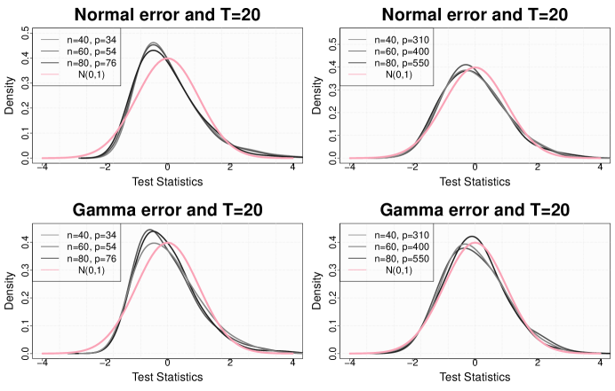
Figure 1: Density curves of the sampling distribution of the proposed test statistic (green lines) and the standard normal distribution (red line).

For the empirical powers, since the underlying model is indeed a simple linear model, we expect the ZC test to have more power under correct model specification than our test. From Table 1, we see that for the non-sparse alternative, the powers are quite high and close to each other for the two tests; the powers are comparable for two error distributions. Under the sparse alternative, both tests have substantial power loss when the dimension is much larger than the sample size indicating that both the mdd and ZC tests target for dense alternatives. Overall, our test is highly comparable to the ZC test under the simple linear model.

Example 4.2.

The second experiment is designed to evaluate the performance of the tests under non-linear model:

$$Y_{i}=\sqrt{\sum^{p}_{j=1}\beta_{j}x_{ij}^{2}}+\epsilon_{i},\quad i=1,2,\dots,n,$$

where the covariates $X_{i}=(x_{i1},x_{i2},...,x_{ip})^{T}$ are generated from the following model:

$$x_{ij}=(\varsigma_{ij}+\varsigma_{i0})/\sqrt{2},\quad j=1,2,...,p,$$ (17)

where $(\varsigma_{i0},\varsigma_{i1},\dots,\varsigma_{ip})^{T}\overset{i.i.d.}{\sim}N(0,I_{p+1})$. Hence the covariates are strongly correlated with the pairwise correlation equal to 0.5. We consider three configurations for the error, $N(0,1)$, $t_{3}$, and $\chi^{2}-1$ respectively.

Under the null, we set $\beta=(\beta_{1},\dots,\beta_{p})^{T}=\mathbf{0}_{p\times 1}$. Under the non-sparse alternative, we set $\beta_{j}=\mathbf{1}\{1\leq j\leq\lfloor n/2\rfloor\}$. For the sparse alternative, $\beta_{j}=\mathbf{1}\{1\leq j\leq 5\}$. We consider $n=100$ and $p=50,100,200$.

Table 2 reports the empirical size and power for the two tests. The size phenomenon is very similar to that of Example 4.1. Under the alternatives, the mdd test consistently outperforms the ZC test in all cases. We observe that under the nonlinear model, the ZC test exhibits very low powers. By contrast, our proposed test is much more powerful (especially in the nonsparse case) regardless of $p$ and the error distribution.

4.2 Conditional quantile independence

In this subsection, we carry out additional simulations to evaluate the performance of the proposed test for conditional quantile independence.

Example 4.3.

Consider the following mixture distribution:

$$Y=(1+Z)\cdot\epsilon-(1+X^{T}\beta)\cdot(1-\epsilon)$$

where $\epsilon$ is a Bernoulli random variable with success probability 0.5; $Z$ is from Gamma(2,2) and $X$ has $p$ components generated from i.i.d Gamma(6,1).

Here $\beta=\mathbf{0}_{p\times 1}$ under the null and it is positive for some components under the alternative. Hence $Y$ has a mixture distribution with half probability to be positive or negative. We also consider non-sparse and sparse alternative and fix $|\beta|_{p}=0.06$ as in Example 4.1. We set $p=50,100,200$, $n=100$ and consider three different quantile levels, $\tau=0.25,0.5,0.75$.

It is not difficult to see that when $\beta=0$, $Y$ and $X$ are independent at all quantile levels; when $\beta\not=0$, $Y$ is conditionally quantile independent of $X$ only when $\tau\geq 0.5$. Furthermore, when $\beta\not=0$, the local quantile independence described in Assumption 3.2 is satisfied when $\tau=0.75$, but does not hold at $\tau=0.5$. As presented in Table 3, our proposed test demonstrates nontrivial power only at quantile level 0.25 under both the sparse and non-sparse alternative, which is consistent with the theory.

Example 4.4.

This example considers a simple model with heteroscedasticity:

$$Y_{i}=\left(1+X_{i}^{T}\beta\right)^{2}\epsilon_{i}$$

where $X_{i}=(x_{i1},x_{i2},\dots,x_{ip})^{T}$ is a $p$-dimensional vector of covariates generated as in (17) and $\epsilon_{i}$ is the error independent of $X_{i}$. All the other configurations are the same as Example 4.2.

We examine the sizes and powers under both non-sparse alternatives and sparse alternatives with four different error distributions, i.e., $N(0,1)$, $t_{3}$, Cauchy(0,1) and $\chi^{2}_{1}-1$. We are interested in testing the conditional quantile independence at $\tau=0.25,0.5,0.75$. Consider $p=50,100,200$, and $n=100$. For the purpose of comparison, we also include the results using our MDD-based test for conditional mean independence. Note that when $\beta$ is nonzero, conditional quantile independence only holds at $\tau=0.5$ for the errors of three types (Normal, Student-t and Cauchy), while conditional quantile dependence is present for other combinations of quantile levels and error distributions. Further note that the local quantile independence assumption (Assumption 3.2) does not hold when $\beta\not=0$ and $\tau=0.5$.

Table 4 shows the empirical sizes and powers for various configurations. The sizes are generally precise at 10% level and slightly inflated at 5% level under $H_{0}$, and they do not seem to depend on the error distribution much. The empirical powers apparently depend on the error distribution. For symmetric distributions, $N(0,1)$, $t_{3}$ and Cauchy(0,1) error, they have comparable powers at $\tau=0.25$ and $0.75$. The powers suffer big reduction under sparse alternatives. In contrast, power for $\chi^{2}_{1}-1$ is almost 1 under the non-sparse alternative at $\tau=0.25$ and remains high even under sparse alternative; at $\tau=0.75$, the proposed test has moderate power in the non-sparse case and suffers a great power loss in the sparse case. This phenomenon may be related to the fact that the chi-square distribution is skewed to the right. At $\tau=0.5$, we observe a significant upward size distortion for all the three symmetric distribution (i.e., Normal, student-$t$ and Cauchy), where the conditional median does not depend on the covariates (i.e., under the null). We speculate that this size distortion is related to the violation of local quantile independence in Assumption 3.2, and indicates the necessity of Assumption 3.2 in obtaining the weak convergence of our test statistics to the standard normal distribution. For non-symmetric distribution (Chi-square), the power is satisfactory at the median.

In comparison, the MDD-based test for conditional mean has power close to the level for $N(0,1)$, $t_{3}$ and $\chi^{2}_{1}-1$ as the covariates only contribute to the conditional variance of the response but not to the conditional mean. In addition, when the mean does not exist, for example in the Cauchy(0,1) case, we observe that the MDD-based test for conditional mean has very little power. Therefore, the test for the conditional quantile dependence can be a good complement to the conditional mean independence test, especially for models that exhibit conditional heteroscedasticity and heavy tail.

4.3 Wild bootstrap

In this section, we implement the Wild bootstrap proposed in Section 2.4. We again consider Example 4.1 under the null of $\beta=\mathbf{0}_{p\times 1}$ in Section 4.1. The results are summarized in Table 5, where we compare the type I errors delivered by normal approximation (mdd) with the wild bootstrap (Boot) approach. It is observed that the size is usually more accurate using wild bootstrap. This is not surprising as it is known in the literature that application of bootstrap method to pivotal statistic has better asymptotic properties, e.g., faster rate of convergence of the actual significance level to the nominal significance level, see the discussions in Westfall and Young (1993). To understand whether the bootstrap distribution is mimicking the finite sample distribution of our test statistics under the null, we also provide in Figure 2 the histograms of the p-values corresponding to the wild bootstrap. As we can see from these histograms, the p-values are close to being uniformly distributed between 0 and 1 indicating the bootstrap distribution is consistently approximating the null distribution of the test statistics.

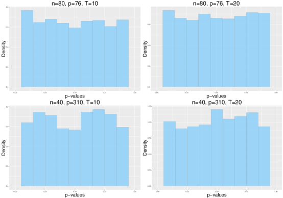
Figure 2: Histograms of the p-values of the test statistics using the studentized bootstrap critical value.

5 Conclusion

In this paper, we proposed new tests for testing conditional mean and conditional quantile independence in the high dimensional setting, where the number of covariates is allowed to grow rapidly with the sample size. Our test statistics are built on the MDD, a recently proposed metric for quantifying conditional mean dependence, and do not involve any tuning parameters. A distinctive feature of our test is that it is totally model free and is able to capture nonlinear dependence which cannot be revealed by using traditional linear dependence metric. Our test for conditional mean independence can be viewed as a nonparametric model-free counterpart of Zhong and Chen’s test, which was developed for high dimensional linear models with homoscedastic errors; our test for conditional quantile independence seems to be the first simultaneous test proposed in the high dimensional setting that detects conditional quantile dependence. Besides the methodological advance, our theoretical analysis reveals a key assumption generally needed in establishing the asymptotic normality for a broad class of $U$-statistic based tests in high dimension, and shed light on the asymptotic theory for high dimensional $U$-statistic.

Our analysis of local asymptotic power shows that our test is less powerful than Zhong and Chen’s test when the high dimensional linear model holds, but the efficiency loss is fairly moderate. As a tradeoff, our test for conditional mean dependence achieves great robustness against model mis-specification, under which the power of Zhong and Chen’s test can greatly deteriorate, as we demonstrate in our simulations. In particular, the proposed conditional mean dependence test can significantly outperform the modified $F$-test in Zhong and Chen (2011) when the underlying relationship between $Y$ and $X$ is nonlinear. Since there seem no well-developed methods yet to check the validity of a high dimensional linear model and it is often unknown whether the response is linearly related to covariates, it might be safe and more reliable to apply our model-free dependence test in practice.

To conclude, we point out a few future research directions. Firstly, given a set of variables $\mathcal{X}^{*}$ which are believed to have significant impact on the response $Y$, it is of interest to test whether the conditional mean or quantile of $Y$ depends on another set of variables $\mathcal{X}$, adjusting for the effect of $\mathcal{X}^{*}$. Based on the recently proposed concept of partial MDD [Park et al. (2015)], we expect that the results could be extended to test the conditional mean or quantile dependence controlling for a set of significant variables. Secondly, we only handle a single quantile level in our test, and it would be interesting to extend our test to testing conditional quantile independence over a range of quantile levels, say $[\tau_{1},\tau_{2}],$ where $0<\tau_{1}<\tau_{2}<1$. Thirdly, the studentized wild bootstrap showed great promise in reducing the size distortion associated with normal approximation in Section 4.3, but there is yet any theory that states the second order accuracy for the wild bootstrap approach. Fourthly, our MDD-based tests mainly target the marginal conditional mean dependence and may fail to capture conditional mean dependence at higher order, which needs to be taken into account in developing new tests. Finally, our test statistics are of $L^{2}$-type, and it may be of interest to develop a $L^{\infty}$-version, which targets for sparse and strong alternatives. We leave these topics for future research.

Acknowledgments. The authors would like to thank the Associate Editor and the reviewers for their constructive comments and helpful suggestions, which substantially improved the paper. We also thank Dr. Ping-Shou Zhong for providing the data set and the R codes used in our simulation studies and data illustration. We are also grateful to Dr. Min Qian for providing us with the matlab code for the tests in McKeague and Qian (2015).

SUPPLEMENTARY MATERIAL

This supplement contains proofs of the main results in the paper, extension to factorial designs, additional discussions and numerical results.

Table 1: Empirical sizes and powers of the MDD-based test for conditional mean independence and the ZC test at significance levels 5% and 10% for Example 4.1.

				Normal error				Gamma error
				mdd		ZC		mdd		ZC
$T$	case	$n$	$p$	5%	10%	5%	10%	5%	10%	5%	10%
$10$	$H_{0}$	40	34	0.069	0.125	0.073	0.116	0.055	0.095	0.055	0.094
		60	54	0.075	0.115	0.068	0.114	0.072	0.118	0.067	0.113
		80	76	0.069	0.114	0.075	0.107	0.063	0.101	0.056	0.100
		40	310	0.043	0.088	0.048	0.092	0.049	0.093	0.053	0.088
		60	400	0.060	0.104	0.058	0.106	0.052	0.098	0.054	0.097
		80	550	0.060	0.106	0.065	0.107	0.047	0.090	0.047	0.082
	non-sparse $H_{a}$	40	34	0.634	0.714	0.678	0.746	0.672	0.748	0.704	0.766
		60	54	0.781	0.833	0.814	0.866	0.803	0.846	0.817	0.871
		80	76	0.848	0.901	0.875	0.914	0.866	0.908	0.883	0.915
		40	310	0.262	0.354	0.287	0.392	0.276	0.391	0.317	0.419
		60	400	0.385	0.489	0.410	0.530	0.386	0.516	0.406	0.523
		80	550	0.435	0.544	0.473	0.574	0.454	0.567	0.474	0.586
	sparse $H_{a}$	40	34	0.310	0.396	0.337	0.411	0.331	0.410	0.357	0.435
		60	54	0.313	0.411	0.344	0.435	0.368	0.455	0.375	0.459
		80	76	0.350	0.442	0.354	0.436	0.343	0.427	0.368	0.449
		40	310	0.067	0.134	0.086	0.145	0.081	0.157	0.088	0.157
		60	400	0.110	0.176	0.108	0.182	0.098	0.161	0.094	0.174
		80	550	0.102	0.171	0.110	0.171	0.093	0.157	0.096	0.167
$20$	$H_{0}$	40	34	0.069	0.114	0.081	0.118	0.063	0.107	0.062	0.090
		60	54	0.068	0.100	0.076	0.108	0.052	0.089	0.058	0.093
		80	76	0.058	0.102	0.059	0.100	0.073	0.111	0.072	0.114
		40	310	0.057	0.098	0.063	0.101	0.077	0.105	0.062	0.096
		60	400	0.061	0.089	0.071	0.099	0.045	0.092	0.046	0.096
		80	550	0.070	0.104	0.074	0.107	0.054	0.100	0.059	0.099
	non-sparse $H_{a}$	40	34	0.976	0.984	0.985	0.990	0.971	0.979	0.977	0.985
		60	54	1.000	1.000	1.000	1.000	0.997	0.998	0.998	0.999
		80	76	1.000	1.000	1.000	1.000	1.000	1.000	1.000	1.000
		40	310	0.848	0.903	0.877	0.918	0.858	0.893	0.877	0.917
		60	400	0.947	0.967	0.961	0.981	0.946	0.973	0.955	0.976
		80	550	0.990	0.994	0.994	0.996	0.981	0.990	0.983	0.990
	sparse $H_{a}$	40	34	0.705	0.763	0.737	0.782	0.715	0.779	0.741	0.786
		60	54	0.743	0.808	0.764	0.821	0.753	0.812	0.768	0.819
		80	76	0.764	0.813	0.782	0.835	0.743	0.799	0.765	0.819
		40	310	0.137	0.212	0.156	0.236	0.185	0.274	0.193	0.269
		60	400	0.186	0.268	0.209	0.275	0.183	0.283	0.195	0.285
		80	550	0.176	0.271	0.200	0.291	0.208	0.288	0.213	0.289

Table 2: Empirical sizes and powers of the MDD-based test for conditional mean independence and the ZC test at significance levels 5% and 10% for Examples 4.2.

			mdd		ZC
error	case	$p$	5%	10%	5%	10%
$N(0,1)$	$H_{0}$	50	0.078	0.112	0.075	0.098
		100	0.075	0.111	0.078	0.109
		200	0.065	0.091	0.062	0.089
	non-sparse $H_{a}$	50	0.927	0.990	0.200	0.221
		100	0.970	0.997	0.213	0.238
		200	0.980	0.998	0.230	0.249
	sparse $H_{a}$	50	0.428	0.583	0.143	0.176
		100	0.370	0.519	0.147	0.172
		200	0.331	0.477	0.129	0.161
$t_{3}$	$H_{0}$	50	0.084	0.110	0.080	0.104
		100	0.075	0.106	0.072	0.097
		200	0.082	0.112	0.063	0.091
	non-sparse $H_{a}$	50	0.759	0.877	0.178	0.206
		100	0.870	0.955	0.182	0.209
		200	0.939	0.983	0.199	0.226
	sparse $H_{a}$	50	0.246	0.355	0.108	0.141
		100	0.208	0.302	0.105	0.136
		200	0.209	0.311	0.108	0.131
$\chi^{2}_{1}-1$	$H_{0}$	50	0.083	0.114	0.083	0.110
		100	0.061	0.096	0.058	0.086
		200	0.058	0.084	0.047	0.078
	non-sparse $H_{a}$	50	0.838	0.937	0.162	0.202
		100	0.933	0.983	0.198	0.226
		200	0.967	0.995	0.216	0.245
	sparse $H_{a}$	50	0.269	0.384	0.113	0.150
		100	0.247	0.364	0.124	0.155
		200	0.233	0.323	0.111	0.141

Table 3: Empirical sizes and powers of the MDD-based test for conditional quantile independence at significance levels 5% and 10% for Example 4.3.

		$H_{0}$		Non-sparse $H_{0}/H_{a}$		Sparse $H_{0}/H_{a}$
$\tau$	$p$	5%	10%	5%	10%	5%	10%
0.25	50	0.054	0.104	0.522	0.644	0.554	0.663
	100	0.048	0.094	0.322	0.464	0.352	0.473
	200	0.044	0.100	0.231	0.368	0.230	0.349
0.50	50	0.058	0.106	0.071	0.129	0.069	0.130
	100	0.047	0.093	0.062	0.104	0.059	0.104
	200	0.056	0.093	0.065	0.104	0.058	0.107
0.75	50	0.050	0.108	0.050	0.108	0.050	0.108
	100	0.058	0.103	0.058	0.103	0.058	0.103
	200	0.067	0.120	0.067	0.120	0.067	0.120

Table 4: Empirical sizes and powers of the MDD-based test for conditional quantile independence at significance levels 5% and 10% for Example 4.4.

			$N(0,1)$		$t_{3}$		Cauchy(0,1)		$\chi^{2}_{1}-1$
$\tau$	case	$p$	5%	10%	5%	10%	5%	10%	5%	10%
0.25	$H_{0}$	50	0.084	0.112	0.058	0.077	0.073	0.094	0.074	0.099
		100	0.073	0.104	0.067	0.094	0.069	0.101	0.071	0.099
		200	0.064	0.085	0.058	0.095	0.062	0.082	0.069	0.094
	non-sparse $H_{a}$	50	0.573	0.640	0.494	0.554	0.368	0.424	0.999	0.999
		100	0.840	0.864	0.727	0.778	0.578	0.632	1.000	1.000
		200	0.936	0.956	0.925	0.941	0.842	0.880	1.000	1.000
	sparse $H_{a}$	50	0.207	0.243	0.146	0.196	0.122	0.162	0.951	0.970
		100	0.198	0.240	0.154	0.196	0.125	0.161	0.956	0.967
		200	0.199	0.235	0.174	0.224	0.125	0.168	0.952	0.965
0.5	$H_{0}$	50	0.083	0.106	0.076	0.097	0.068	0.099	0.064	0.089
		100	0.072	0.100	0.063	0.087	0.057	0.092	0.062	0.091
		200	0.073	0.100	0.053	0.073	0.071	0.095	0.063	0.088
	non-sparse $H_{0}/H_{a}$	50	0.110	0.145	0.093	0.125	0.091	0.127	0.704	0.755
		100	0.151	0.184	0.123	0.168	0.126	0.169	0.862	0.888
		200	0.230	0.274	0.232	0.269	0.196	0.242	0.939	0.953
	sparse $H_{0}/H_{a}$	50	0.083	0.110	0.075	0.100	0.077	0.099	0.234	0.288
		100	0.079	0.108	0.063	0.088	0.066	0.107	0.252	0.299
		200	0.077	0.109	0.057	0.085	0.079	0.098	0.242	0.303
0.75	$H_{0}$	50	0.067	0.098	0.080	0.108	0.062	0.084	0.065	0.085
		100	0.057	0.085	0.078	0.098	0.076	0.111	0.073	0.095
		200	0.064	0.095	0.063	0.085	0.069	0.095	0.065	0.088
	non-sparse $H_{a}$	50	0.585	0.638	0.516	0.577	0.384	0.445	0.129	0.161
		100	0.834	0.875	0.744	0.800	0.587	0.645	0.199	0.233
		200	0.944	0.961	0.925	0.940	0.824	0.865	0.329	0.385
	sparse $H_{a}$	50	0.187	0.235	0.191	0.232	0.131	0.168	0.076	0.096
		100	0.193	0.237	0.197	0.236	0.131	0.172	0.092	0.116
		200	0.195	0.244	0.167	0.213	0.135	0.170	0.078	0.109
mean	$H_{0}$	50	0.071	0.103	0.069	0.101	0.067	0.098	0.052	0.097
		100	0.074	0.101	0.075	0.097	0.071	0.101	0.060	0.103
		200	0.067	0.094	0.078	0.105	0.066	0.088	0.054	0.096
	non-sparse $H_{a}$	50	0.077	0.107	0.071	0.107	0.109	0.144	0.058	0.107
		100	0.077	0.102	0.063	0.091	0.117	0.143	0.057	0.107
		200	0.076	0.109	0.078	0.117	0.146	0.166	0.059	0.102
	sparse $H_{a}$	50	0.072	0.103	0.066	0.102	0.080	0.110	0.057	0.094
		100	0.067	0.100	0.059	0.084	0.080	0.105	0.060	0.112
		200	0.068	0.102	0.075	0.108	0.091	0.116	0.053	0.095

Table 5: Size comparison for the proposed test using the normal approximation (mdd) and the wild bootstrap approximation for Example 4.1

			Normal error				Gamma error
			5%		10%		5%		10%
$T$	$n$	$p$	mdd	Boot	mdd	Boot	mdd	Boot	mdd	Boot
$10$	40	34	0.069	0.055	0.125	0.109	0.055	0.044	0.095	0.087
	60	54	0.075	0.068	0.115	0.113	0.072	0.053	0.118	0.115
	80	76	0.069	0.053	0.114	0.106	0.063	0.048	0.101	0.093
	40	310	0.043	0.037	0.088	0.083	0.049	0.046	0.093	0.085
	60	400	0.060	0.053	0.104	0.101	0.052	0.052	0.098	0.096
	80	550	0.060	0.058	0.106	0.101	0.047	0.039	0.090	0.090
$20$	40	34	0.069	0.059	0.114	0.103	0.063	0.048	0.107	0.097
	60	54	0.068	0.056	0.100	0.092	0.052	0.035	0.089	0.081
	80	76	0.058	0.040	0.102	0.094	0.073	0.051	0.111	0.106
	40	310	0.057	0.046	0.098	0.091	0.077	0.064	0.105	0.097
	60	400	0.061	0.053	0.089	0.088	0.045	0.039	0.092	0.088
	80	550	0.070	0.056	0.104	0.093	0.054	0.044	0.100	0.091

References

- [1] Chen, S. X. and Qin, Y. (2010). A two sample test for high dimensional data with applications to gene-set testing. Ann. Statist. 38 808-835.
- [2] Efron, B. and Tibshirani, R. (2007). On testing the significance of sets of genes. Ann. Appl. Stat. 1 107-129.
- [3] Fan, J. and Lv, J. (2008) Sure independence screening for ultra-high dimensional feature space (with discussion) J. Roy. Stat. Soc. Ser. B. 70 849-911.
- [4] Fang, K., Kotz, S. and Ng, K.-W. (1990). Symmetric Multivariate and Related Distributions. Chapman & Hall, London.
- [5] Feng, L., Zou, C. and Wang, Z. (2013). Rank-based score tests for high-dimensional regression coefficients. Electron. J. Stat. 7 2131-2149.
- [6] Goeman, J., van de Geer, S. A. and van Houwelingen, H. C. (2006). Testing against a high dimensional alternative. J. R. Statist. Soc. B. 68 477-493.
- [7] Hall, P. (1984). Central limit theorem for integrated square error of multivariate nonparametric density estimators. J. Multivariate Anal. 14 1-16.
- [8] Hall, P. and Heyde, C. C. (1980). Martingale Limit Theory and Its Application. Academic Press, New York.
- [9] He, X., Wang, L. and Hong, H. (2013). Quantile-adaptive model-free nonlinear feature screening for high-dimensional heterogeneous data. Ann. Statist. 41 342-369.
- [10] Koenker, R. and Bassett, G. (1978). Regression quantiles. Econometrica. 46 33-50.
- [11] Lan, W., Wang, H. and Tsai, C. L. (2014). Testing covariates in high-dimensional regression. Ann. Inst. Statist. Math. 66 279-301.
- [12] Li, Q., Hsiao, C. and Zinn, J. (2003). Consistent specification tests for semiparametric/nonparametric models based on series estimation methods. Journal of Econometrics. 112 295-325.
- [13] Liu, J., Zhong, W. and Li, R. (2015) A selective overview of feature screening for ultrahigh-dimensional data. Science China Mathematics. 58 2033-2054.
- [14] Lkhagvadorj, S., Qu, L., Cai, W., Couture, O., Barb, C., Hausman, G., Nettleton, D., Anderson, L., Dekkers, J. and Tuggle, C. (2009). Microarray gene expression profiles of fasting induced changes in liver and adipose tissues of pigs expressing the melanocortin-4 receptor D298N variant. Physiological Genomics. 38 98-111.
- [15] McKeague, I. W. and Qian, M. (2015) An adaptive resampling test for detecting the presence of significant predictors. J. Amer. Statist. Assoc. 110 1422-1433.
- [16] Newton, M., Quintana, F., Den Boon, J., Sengupta, S. and Ahlquist, P. (2007). Random-set methods identify distinct aspects of the enrichment signal in gene-set analysis. Ann. Appl. Stat. 1 85-106.
- [17] Park, T., Shao, X. and Yao, S. (2015). Partial martingale difference correlation. Electron. J. Stat. 9 1492-1517.
- [18] Sejdinovick, D., Sriperumbudur, B., Gretton, A. and Fukumizu, K. (2013). Equivalence of distance-based and RKHS-based statistics in hypothesis testing. Ann. Statist. 41 2263-2291.
- [19] Serfling, R. J. (1980). Approximation Theorems of Mathematical Statistics. Wiley, New York.
- [20] Shao, X. and Zhang, J. (2014). Martingale difference correlation and its use in high dimensional variable screening. J. Amer. Statist. Assoc. 109 1302-1318.
- [21] Subramanian, A., Mootha, V. K., Mukherjee, S., Ebert, B. L., Gillette, M. A., Paulovich, A., Pomeroy, S. L., Golub, T. R., Lander, E. S. and Mesirov, J. P. (2005). Gene set enrichment analysis: a knowledge-based approach for interpreting genome-wide expression profiles. Proc. Natl. Acad. Sci. USA 102 15545-15550
- [22] Székely, G. J. and Rizzo, M. L. (2013). The distance correlation t-test of independence in high dimension. J. Multivariate Anal. 117 193-213.
- [23] Székely, G. J. and Rizzo, M. L. (2014). Partial distance correlation with methods for dissimilarities. Ann. Statist. 42 2382-2412.
- [24] Székely, G. J., Rizzo, M. L. and Bakirov, N. K. (2007). Measuring and testing independence by correlation of distances. Ann. Statist. 35 2769-2794.
- [25] Wang, S. and Cui, H. (2013). Generalized F test for high dimensional linear regression coefficients. J. Multivariate Anal. 117 134-149.
- [26] Wang, H. and He, X. (2007). Detecting differential expressions in geneChip microarray studies: A quantile approach. J. Amer. Statist. Assoc. 102 104-112.
- [27] Wang, H. and He, X. (2008). An enhanced quantile approach for assessing differential gene expressions. Biometrics. 64 449-457.
- [28] Wang, L., Wu, Y. and Li, R. (2012). Quantile regression of analyzing heterogeneity in ultra-high dimension. J. Amer. Statist. Assoc. 107 214-222.
- [29] Westfall, P. H. and Young, S. S. (1993). Resampling-based Multiple Testing: Examples and Methods for p-value Adjustment. John Wiley and Sons, New York.
- [30] Wu, C. F. J. and Hamada, M. S. (2009). Experiments Planning, Analysis and Optimization. Wiley, New York.
- [31] Yata, K. and Aoshima, M. (2013). Correlation tests for high-dimensional data using extended cross-data-matrix methodology. J. Multivariate Anal. 117 313-331.
- [32] Zhong, P. S. and Chen, S. X. (2011). Testing for high-dimensional regression coefficients with factorial designs. J. Amer. Statist. Assoc. 106 260-274.